


1. Introduction
Numerous studies have revealed unprecedented global glacier recession during the late 20th and early 21st century, which has been linked to anthropogenically-induced climate change (e.g. Haeberli and others, Reference Haeberli, Hoelzle, Paul and Zemp2007; Marzeion and others, Reference Marzeion, Jarosch and Gregory2014; Zemp and others, Reference Zemp2015). Although there has been a significant mass loss from the large polar ice sheets (Shepherd and others, Reference Shepherd2012), the combined melt from mountain glaciers and ice caps between 2003 and 2009 accounted for 29 ± 13% of observed sea level rise, approximately equal to the loss from both the Greenland and Antarctic ice sheets (IPCC, 2013). Furthermore, it has been proposed that the combined melt from ‘uncharted glaciers’ (i.e. glaciers that are not currently included in global glacier inventories) may account for as much as 42.7 mm (31% of a total 137.1 mm sea level equivalent from glaciers globally, excluding the Greenland and Antarctic ice sheets) of sea level rise between 1901 and 2015 (Parkes and Marzeion, Reference Parkes and Marzeion2018).
The development of satellite remote sensing over the last 30–40 years revolutionised our ability to map and monitor glacier extent, reducing a previous reliance on historical records or field-based measurements of glacier change (Andreassen and others, Reference Andreassen, Elvehøy and Kjøllmoen2002; Pellikka and Rees, Reference Pellikka and Rees2009). Moreover, recent advances in satellite technology and data availability have dramatically improved the spatial, temporal and spectral resolution of imagery (Roy and others, Reference Roy, Behera and Srivastav2017). A clear example of this is the Swiss Glacier Inventory SGI2010 which was derived from the manual mapping of 0.25 m resolution aerial orthophotographs (Fischer and others, Reference Fischer, Huss, Barboux and Hoelzle2014). Other recent glacier inventories such as the Inventory of Norwegian Glaciers (Andreassen and others, Reference Andreassen, Winsvold, Paul, Hausberg, Andreassen and Winsvold2012b) have also utilised orthophotographs as a means of validating their glacier maps which were compiled from satellite imagery.
Prompted in part by the Global Land Ice Measurements from Space (GLIMS) initiative, there has been a large body of work assessing which remote-sensing techniques are most appropriate for mapping glaciers in different settings (Racoviteanu and others, Reference Racoviteanu, Paul, Raup, Khalsa and Armstrong2009; Paul and others, Reference Paul2010, Reference Paul2013; Raup and Khalsa, Reference Raup and Khalsa2010). However, there has been less focus on very small glaciers (generally considered to be <0.5 km2), sometimes referred to as ‘glacierets’ (Lliboutry, Reference Lliboutry1964–1965; WGMS, Reference Haeberli, Bösch, Scherler, Østrem and Wallén1989; Cogley and others, Reference Cogley2011), ice aprons (Benn and Evans, Reference Benn and Evans2010) and/or ‘niche glaciers’ (Groom, Reference Groom1959; Grove, Reference Grove1961), with various (and sometimes conflicting) definitions regarding the classification and mapping of these units (Fischer, Reference Fischer2018). Despite their small area, however, mapping very small glaciers is important for several reasons. First, their widespread distribution and frequent occurrence mean they likely account for ~80–90% of the total number of glaciers located in mid- to low-latitude mountain ranges (Fischer and others, Reference Fischer, Huss, Barboux and Hoelzle2014; Paul and Mölg, Reference Paul and Mölg2014; Pfeffer and others, Reference Pfeffer2014; Huss and Fischer, Reference Huss and Fischer2016). Second, very small glaciers act as a reservoir for water storage, moderating interannual variability in streamflow constituting a significant part of the hydrological system in mountain areas (Barnett and others, Reference Barnett, Adam and Lettenmaier2005) and, with a warming climate, are critical in terms of increasing concern about future water security (Huss, Reference Huss2011; Rangecroft and others, Reference Rangecroft2013; Huss and Fischer, Reference Huss and Fischer2016). Third, smaller glaciers are highly sensitive to climate change and typically exhibit the shortest response times to a given climate forcing (Grudd, Reference Grudd1990; Oerlemans, Reference Oerlemans1994; Nesje and others, Reference Nesje, Bakke, Dahl, Lie and Matthews2008; Federici and Pappalardo, Reference Federici and Pappalardo2010). However, they can also be disproportionately influenced by local topography, such that when they survive in heavily-shaded cirques, they may be sustained for longer than expected (Demuth and others, Reference Demuth2008; DeBeer and Sharp, Reference DeBeer and Sharp2009; Evans, Reference Evans2009). Fourth, monitoring the evolution of very small glaciers could reveal new insights regarding their fate over longer time-scales, e.g. their disappearance versus transitioning into debris-covered and/or rock glaciers, which may also have implications for catchment hydrology (Capt and others, Reference Capt, Bosson, Fischer, Micheletti and Lambiel2016; Jones and others, Reference Jones2018a, Reference Jones, Harrison, Anderson and Betts2018b, Reference Jones, Harrison, Anderson and Whalley2019). Finally, it is important to correctly classify very small glaciers because of their relevance to issues of environmental protection in some parts of the world, especially where they may exist within national parks (Fraser, Reference Fraser2017; Tollefson and Rodríguez-Mega, Reference Tollefson and Rodríguez-Mega2017).
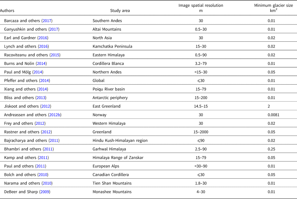
Despite their importance and ubiquity, there is very little guidance on how to distinguish very small glaciers (<0.5 km2) from perennial snowpatches when compiling remotely sensed glacier inventories or change assessments. In practice, most researchers simply define a minimal size-threshold, commonly somewhere between 0.05 and 0.01 km2 (Table 1). All units below this size-threshold are then ignored or removed, due to the large uncertainty in differentiating between snowpatches and glaciers (Lindh, Reference Lindh1984; Paul and Mölg, Reference Paul and Mölg2014; Lynch and others, Reference Lynch, Barr, Mullan and Ruffell2016). This approach is likely to be appropriate for coarse to medium resolution satellite imagery (e.g. Landsat, 80–15 m; Sentinel, 20–10 m), but the last decade has seen a huge growth in much higher resolution satellite imagery (e.g. GeoEye-1, 0.46 m; Planet labs, 3–0.75 m; Pleiades-1, 0.5 m; SPOT, 1.5 m; WorldView, 0.31 m, etc.). Alongside this, there has been an increase in the amount of imagery acquired via Unmanned Aerial Vehicles (UAVs) and, although they only cover small areas, they can provide centimetre-resolution imagery for glacier mapping. These new data sources should therefore permit the identification of very small glaciers, and perhaps render minimum size-thresholds of 0.05–0.01 km2 inappropriate. Indeed, some more recent studies using high-resolution imagery (e.g. 0.25 m) have no minimum size-threshold and, as a result, glaciers as small as ~0.001 km2 have been mapped (Huss and Fischer, Reference Huss and Fischer2016).
Example of minimum size-thresholds used in previous remote-sensing studies mapping glacier changes, listed in chronological order
Given the anticipated growth in high-resolution imagery for glacier mapping, the aim of this paper is to explore ways of improving the objectivity and consistency of mapping very small glaciers (<0.5 km2 and especially those <0.05 km2) on high-resolution satellite imagery and aerial photographs. First, we draw attention to the differences in the area and number of very small glaciers identified when using (a) imagery of varying resolutions and (b) different mapping approaches (automated, semi-automated, manual). This is achieved by analysing satellite imagery and aerial orthophotographs with pixel resolutions from 30 to 0.25 m and applying a range of common approaches for mapping of glaciers. Secondly, we develop new criteria to help the objective identification and mapping of very small glaciers using high-resolution imagery. These criteria are developed with the aim of reducing uncertainty and increasing the accuracy and completeness of glacier inventories where high-resolution imagery is available.
2. Study area
The study area lies within the Kåfjord/Nordreisa municipality, Troms county, northern Norway (Fig. 1). This area was selected because it contains numerous small glaciers and snowpatches, often partially obscured by shadow and some with thin debris cover, making it a particularly challenging environment and therefore suitable for testing approaches to identify and map very small glaciers.
Study site location in Troms county, northern Norway. Red rectangle in (a) represents location of image (b), white rectangle in (b) represents location of image (c), and white star in (b) denotes weather station location at Sørkjosen. Note: (b and c) base image is Landsat 8 scene (path 196, row 11) displayed as a false colour composite (R-G-B; 5-4-3). Panel (c) is 0.25 m resolution 2016 aerial orthophotograph overlain on the Landsat imagery. Numbers in (c) are from the Norwegian Glacier Inventory (NGI).
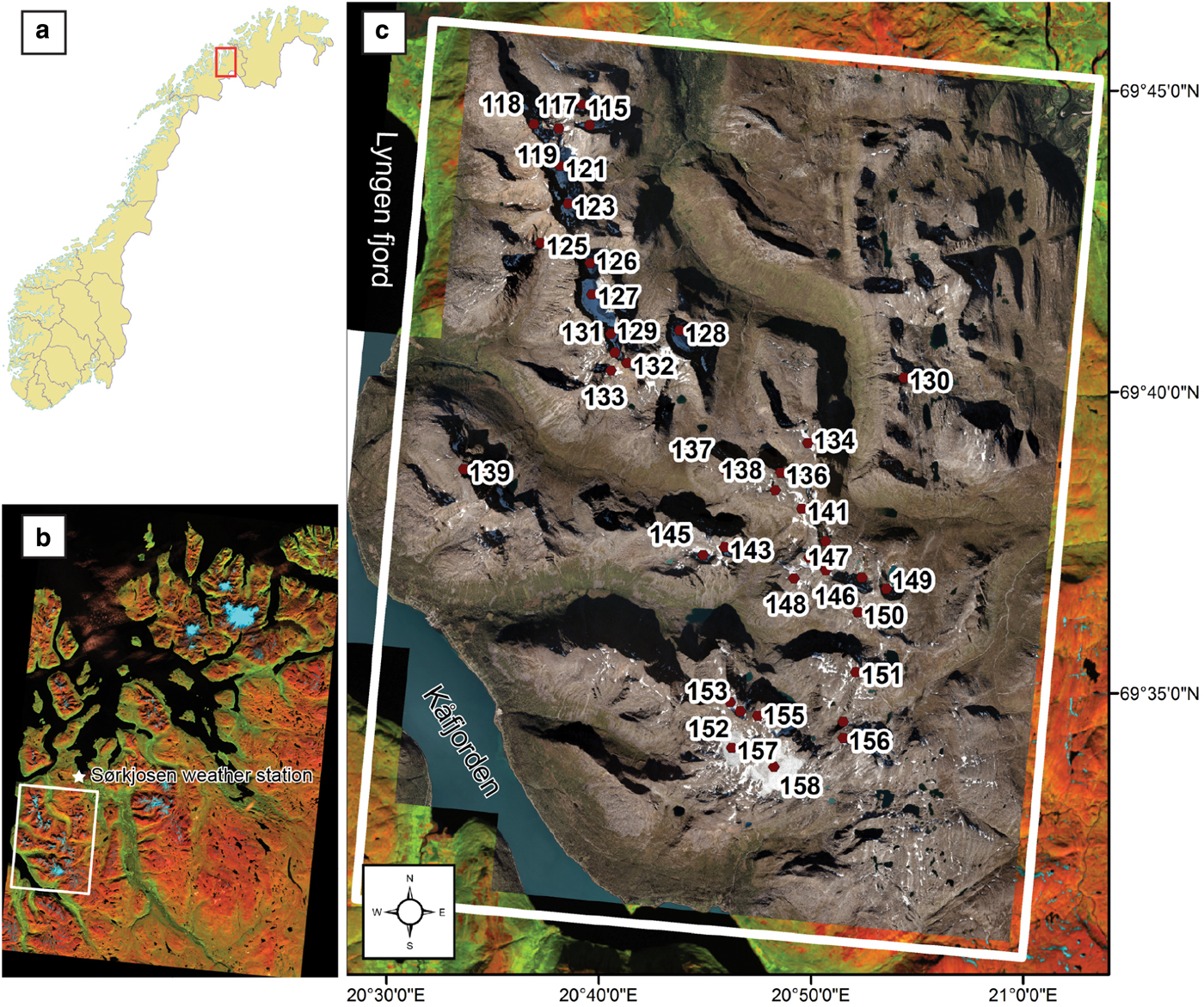
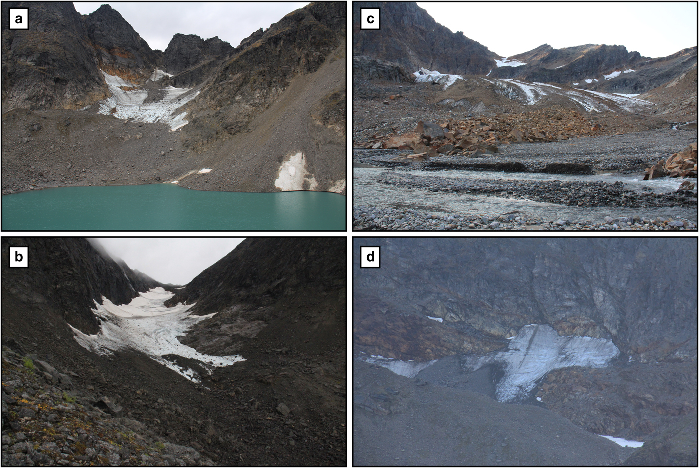
The study area (Fig. 1c) is a minor mountain range, with peaks ranging from 1183 m a.s.l. to 1320 m a.s.l., dominated by valley and cirque-type glaciers within an elevation range of ~600–1200 m a.s.l. Many glaciers tend to exist in sheltered and shadowed locations, with generally thin (<1 m) and patchy debris cover on some termini (Fig. 2). To the west is a major fjord system (Lyngen Fjord) and there are subsidiary fjords to the north and south. The glaciers are subject to a maritime climate. As such, they are particularly sensitive to climate fluctuations (De Woul and Hock, Reference De Woul and Hock2005) and their mass balance is heavily influenced by variations in the Arctic Oscillation (Andreassen and others, Reference Andreassen, Kjøllmoen, Rasmussen, Melvold and Nordli2012a; Kjøllmoen and others, Reference Kjøllmoen, Andreassen, Elvehøy and Jackson2018). Precipitation primarily falls as snow between October and May, while rainfall can occur throughout the year (Vikhamar-Schuler and others, Reference Vikhamar-Schuler, Hanssen-Bauer and Førland2010). Average monthly temperature typically varies from −10 to 15°C, with the hottest months (June to September) reaching average daily highs of up to 16°C (station number 91740, 6 m a.s.l: http://www.eKlima.no).
An example of the type of glaciers within the study area, which are partly obscured by debris cover. Images (a, b, and c) show glaciers 115, 117 and 121, respectively (Andreassen and others, Reference Andreassen, Winsvold, Paul, Hausberg, Andreassen and Winsvold2012b). Image (d) shows a very small (~0.03 km2) glacier, not included within the NGI. All users mapped and classified glaciers (a–c) as certain. Users 1 and 2 mapped and classified the glacier in (d) as certain, but User 3 did not map this unit (see Discussion). Locations shown in Figure 1c.
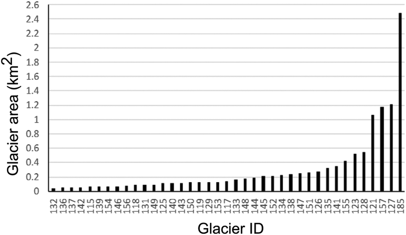
Glaciers in Norway have been mapped by the Norwegian Water Resources and Energy Directorate (NVE) and their characteristics are detailed in the Inventory of Norwegian Glaciers (Andreassen and others, Reference Andreassen, Winsvold, Paul, Hausberg, Andreassen and Winsvold2012b), henceforth referred to as the NGI (Norwegian Glacier Inventory). This most recent glacier inventory was produced using medium-resolution Landsat imagery and a TM3/TM5 band ratio method (Andreassen and others, Reference Andreassen, Paul, Kaab and Hausberg2008; Paul and Andreassen, Reference Paul and Andreassen2009), with all units below 0.0081 km2 excluded from the inventory. The mapped units were manually classified as ‘glaciers’, ‘possible snowfields’ or ‘snow’ and additional manual corrections were made where necessary. Within the study area (Fig. 1c) the NGI records 40 glaciers, with a total glacial extent of 12.09 km2 (Fig. 3), and an additional seven units classified as possible snowfields with a total area of ~0.85 km2 (Andreassen and others, Reference Andreassen, Winsvold, Paul, Hausberg, Andreassen and Winsvold2012b). The recorded glaciers range in size from 2.48 to 0.04 km2 (Andreassen and others, Reference Andreassen, Winsvold, Paul, Hausberg, Andreassen and Winsvold2012b). Only 10% of the glaciers are >1 km2 but they account for ~49% of the total glacial area.
Overview of glacier size distribution within the study site (see Fig. 1) as recorded in the NGI. Only 10% of glaciers are >1 km2 while 85% of glaciers are ⩽0.5 km2.
3. Methods
Obtaining suitable imagery in maritime Norway is challenging. Frequent cloud cover means the number of appropriate satellite scenes each year can be very low (Marshall and others, Reference Marshall, Dowdeswell and Rees1994; Andreassen and others, Reference Andreassen, Paul, Kaab and Hausberg2008). Furthermore, due to the high latitude of this study area, late-lying snow is prevalent, limiting image collection to between July and September. In this study, aerial orthophotographs, Landsat 8 OLI and Sentinel-2A imagery were selected to determine the effect that different image resolutions have on the way that very small glaciers are identified and mapped (Table 2).
List of imagery used in this study and the associated mapping technique
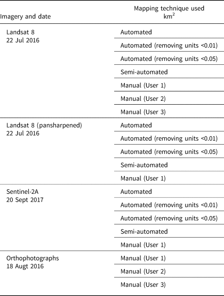
User 1, User 2 and User 3 are each experts with previous glacier mapping experience.
The four most common mapping techniques (automated mapping, automated mapping with a size-threshold, semi-automated mapping and manual mapping) were performed on Landsat 8 OLI (30 m resolution), pan-sharpened Landsat 8 OLI (whereby a 15 m resolution panchromatic image was merged with the 30 m resolution multispectral image to create a single 15 m resolution colour image) and Sentinel-2A (10 m resolution) imagery. Only manual mapping was conducted on the orthorectified aerial photographs (with resolution 0.25 m). Furthermore, because there remains considerable debate about how to define very small glaciers (Fischer, Reference Fischer2018), glaciers were mapped following the definition of Cogley and others (Reference Cogley2011), i.e. a glacier is defined as ‘a perennial mass of ice, and possibly firn and snow … showing evidence of past or present flow’ (Cogley and others, Reference Cogley2011, p. 45). Note that the definition of a glacier by Cogley and others (Reference Cogley2011) was preferred because of the emphasis on evidence of flow, which is different from the GLIMS definition of a glacier whereby "a glacier or perennial snow mass, identified by a single GLIMS glacier ID, consists of a body of ice and snow that is observed at the end of the melt season …’ (Raup and Khalsa, Reference Raup and Khalsa2010, p. 4).
The first approach, automated mapping using a band ratio method (Williams and others, Reference Williams, Hall and Benson1991; Pellikka and Rees, Reference Pellikka and Rees2009), was used on the multispectral satellite imagery. The high reflectivity of ice and snow in the visible and near-infrared wavelengths (VNIR: 0.4–1.2 µm; Bands 1–4 on Landsat 8 OLI) compared to a very low reflectivity in the shortwave infrared (SWIR: 1.4–2.5 µm; Band 5 on Landsat 8 OLI) is used to automatically delineate glacier extents (Racoviteanu and others, Reference Racoviteanu, Paul, Raup, Khalsa and Armstrong2009). Band ratio images were computed in ERDAS Imagine software from the raw multispectral imagery (e.g. OLI Band 3/OLI Band 5) and converted to a binary image (ice/snow classified as 1, remaining surfaces classified as 0; Shapiro and Stockman, Reference Shapiro and Stockman2001). Some researchers also implement an additional threshold (e.g. Band 1) which can sometimes improve mapping in shadowed areas. This approach does not always lead to a marked improvement and it was not used for our assessment. Following the conversion to a binary image, the resulting image was compared against a false colour composite of the multispectral imagery (bands 5, 4 and 3 as Red, Green, Blue) to find the most suitable (albeit subjective) threshold value to isolate glaciers from non-glaciers (Raup and others, Reference Raup2007). A median (3 × 3 kernel) filter was then applied to the binary image to reduce noise from isolated pixels outside the glaciers and to close small voids within the glaciers (such as those created by discontinuous debris cover).
The second mapping approach uses the automatically mapped glacier outlines from approach one to assess the impact of implementing different minimum size-thresholds for glacier inventories. To assess size-thresholds, the automated maps were copied and then all mapped units below a minimum glacier area of (a) 0.05 km2 or (b) 0.01 km2 were removed.
The third approach was semi-automated mapping, also conducted on the multispectral satellite imagery. Initial glacier outlines were generated automatically, as in approach one, and outlines were then manually edited (by a single user) to attempt to correct areas where the automated process had obviously failed to accurately map glacier outlines (usually in association with debris cover, heavy shading or proglacial lakes). Glacier ice was identified using an R-G-B (5-4-3) false colour composite whereby ice has a distinct blue colour (Andreassen and others, Reference Andreassen, Winsvold, Paul, Hausberg, Andreassen and Winsvold2012b). Furthermore, any units that were perceived by the operator to be incorrectly mapped as glaciers were removed, while any glaciers perceived as missing were added by manual digitisation.
The fourth approach, also applied to the multispectral satellite imagery, was manual mapping. Here, all potential glacier units were identified and mapped in ArcMap by a single user drawing a polygon-shapefile around their perceived boundaries. To ensure accuracy in mapping, especially around areas of shade, each individual image was viewed using multiple band combinations of Red-Green-Blue as 5-4-3, 4-3-2 and 3-2-1 (Andreassen and others, Reference Andreassen, Winsvold, Paul, Hausberg, Andreassen and Winsvold2012b). To investigate the impact of subjective interpretation by individual users, different experts with prior experience of mapping glaciers (identified as User 1, User 2 and User 3) undertook manual mapping on the Landsat 8 imagery (see Table 2).
Finally, a manual technique was used to map glacier outlines on the aerial orthophotographs. All glacier units were outlined manually by the three different users as individual polygon-shapefiles.
4. Results
The results of the different mapping techniques applied to different imagery are displayed in Table 3, which also includes summary statistics of the glaciers mapped in the NGI (Andreassen and others, Reference Andreassen, Winsvold, Paul, Hausberg, Andreassen and Winsvold2012b). Note that the NGI data were mapped using a semi-automated approach from Landsat 7 (ETM+) imagery captured in 2001. In part, this explains the difference in the total number of units and size of glaciers mapped, as there are 15–16 years between the acquisition dates of the NGI and this study.
Results of mapping glaciers using multispectral satellite imagery at 30, 15 and 10 m resolution and 0.25 m aerial orthophotographs
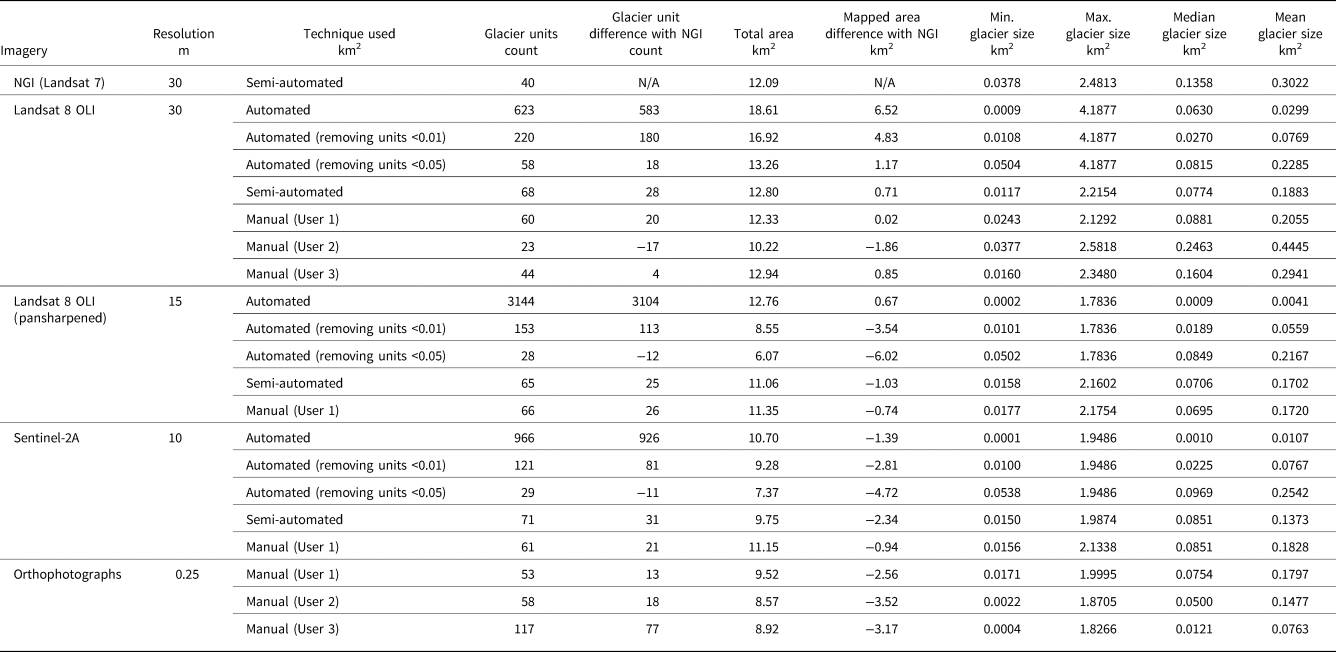
The top row of data is the results of mapping conducted in 2001 taken from the Inventory of Norwegian Glaciers (NGI).
4.1. Satellite imagery
4.1.1. Automated and semi-automated mapping
The unedited automated approach resulted in the highest numbers of mapped glacier units, regardless of image resolution (Table 3). The greatest number of units mapped (n = 3144) were derived from applying the automated approach to the pan-sharpened Landsat 8 (15 m) imagery (Table 3). An increase in the quantity of mapped units did not, however, necessarily equate to a greater total mapped area. For example, the total mapped area of 623 units on the Landsat 8 imagery (30 m) was 18.61 km2, while the total mapped area of 3144 units on the pan-sharpened Landsat 8 (15 m) was 12.76 km2 (Table 3). The automated approach consistently maps the smallest units (glacial and/or non-glacial) across all image resolutions, and the area of the smallest units mapped decreases with increasing image resolution (Table 3). However, the automated approach resulted in a large number of false-positive results, as the majority of units may be outlines of snow or other non-glacial features.
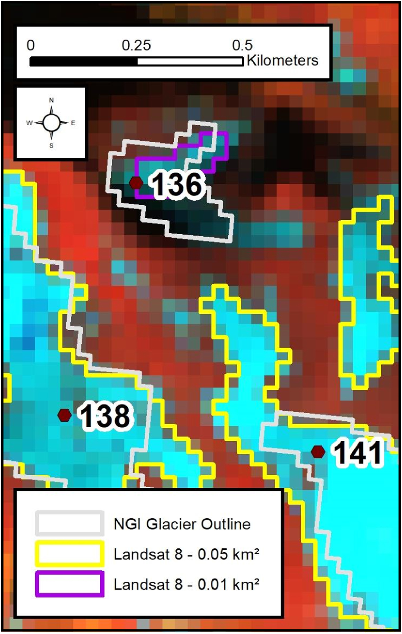
The use of a minimum size-threshold inevitably leads to a reduction in the number of units mapped. Using a minimum size-threshold of 0.01 km2, compared to no minimum size-threshold, resulted in the removal of 403 (Landsat 8), 2991 (pan-sharpened Landsat 8) and 845 (Sentinel-2A) mapped units (Table 3, Fig. 4). Increasing the minimum size-threshold to 0.05 km2 resulted in the removal of 565 (Landsat 8), 3116 (pansharpened Landsat 8) and 937 (Sentinel-2A) mapped units, compared to our results with no minimum size class. A minimum size-threshold clearly reduces the number of units mapped, but only discriminates on the basis of size, rather than genesis, and so may incorrectly eliminate a substantial number of very small glacier units (Fig. 4).
Example where using a 0.05 km2 size-threshold (yellow outlines) eliminates a glacier included in the NGI (no. 136 with an area of 0.0468 km2 in that inventory). A significant proportion of the mapped difference is attributed to the heavy shading over the glacier area meaning it falls outside of the required reflective value for the automated method. Note: where only a yellow outline is seen on glaciers 138 and 141, the purple outline is drawn directly underneath and therefore not visible. Background image: Landsat 8 (30 m resolution, R-G-B as 5-4-3). Location shown in Figure 1.
The semi-automated approach, where automated outputs were manually edited, substantially reduced both the number of glacier units and the total areal extent when compared to the simple automated approaches alone (Table 3). Using the semi-automated approach resulted in the highest number of units on the Sentinel-2A imagery (10 m; 71 units), compared to 68 units on Landsat (30 m) and 65 on pan-sharpened Landsat 8 (15 m) imagery. When comparing the total mapped area from the semi-automated approach, the Sentinel-2A imagery (10 m) gave the smallest total mapped area at 9.75 km2, a reduction in area of 24% and 12% compared to the Landsat 8 and pan-sharpened Landsat 8 imagery (30 and 10 m), respectively (Table 3). The semi-automated approach involved editing by an experienced user, meaning the likelihood of removing actual glacier units is diminished, but it remains highly subjective.
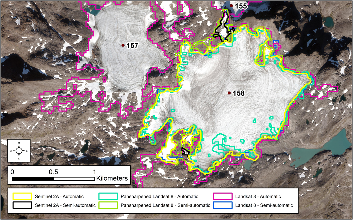
To examine how the above techniques might influence the mapping of both larger and very small glaciers, we separately analysed the outlines of the largest and smallest glaciers found within the study area (as listed in the NGI). The largest NGI glacier in the study site is glacier 158 (Noammerjiehkki) with an area (in 2001) of ~2.48 km2 (Andreassen and others, Reference Andreassen, Winsvold, Paul, Hausberg, Andreassen and Winsvold2012b). When re-mapped using an automated approach, the resulting areal extent was ~4.19 km2 on 2016 Landsat 8 imagery (30 m resolution), ~1.78 km2 on the 2016 pan-sharpened Landsat 8 imagery (15 m) and ~1.95 km2 on 2017 Sentinel-2A imagery (10 m; Fig. 5). The automated approach on the 30 m resolution imagery erroneously merges glacier 158 with adjacent units (glaciers 155 and 157), due to seasonal snow obscuring the boundary of glacier 158 and, therefore, resulting in the large area differences between image resolutions. It is possible for such errors to be manually corrected and units are divided into different entities using glacier basins (Andreassen and others, Reference Andreassen, Winsvold, Paul, Hausberg, Andreassen and Winsvold2012b). Indeed by using a semi-automated approach, users in our study were able to approximate glacier extent beneath the snow cover. Therefore, outlines of glacier 158 derived from different resolution imagery showed far less variance: ~2.22, 2.16 and 1.99 km2 (30, 15 and 10 m resolution imagery, respectively; Fig. 5, Table 3).
The mapped areal extent of glacier 158 (Noammerjiehkki) when applying automated techniques using the band ratio method on multispectral satellite imagery. The automatic approach on the Landsat 8 (30 m) imagery (pink line) results in the merging of glaciers 157, 158 and 155 into one unit with an areal extent of 4.19 km2. Closer inspection suggests a definition of the three as separate units. Note: To emphasise the substantial differences in outlines between the Landsat 8 automated method and all other methods, only the mapped extent of glacier 158 is shown. All other mapped units are removed from this image, e.g. glaciers 155 and 157 are not shown for the other imagery types or mapping techniques. Location shown in Figure 1.
The smallest glacier in the study site according to the NGI is glacier 130 (Fig. 6) with an area (in 2001) of ~0.04 km2 (Andreassen and others, Reference Andreassen, Winsvold, Paul, Hausberg, Andreassen and Winsvold2012b). When re-mapped using an automated approach on 2016 Landsat 8 imagery (30 m), the resulting areal extent is ~0.03 km2, but it is measured at ~0.01 km2 on both the 2016 pan-sharpened (15 m) and 2017 Sentinel-2A imagery (10 m; Fig. 6). The 0.01 km2 size-threshold does not affect this unit but the 0.05 km2 threshold removed it from the map. With a semi-automated approach, the unit is mapped with an area of 0.02 km2 on the 15 and 10 m resolution imagery. However, the unit was not mapped at the 30 m resolution due to the high uncertainty in distinguishing it as a glacier rather than a snowpatch (Fig. 6).
The mapped areal extent of glacier 130 when applying automated and semi-automated techniques using the band ratio method for multispectral satellite imagery. Note that the glacier was removed by the operator using the semi-automatic approach on the Landsat 8 imagery (30 m), presumably because they thought it was a small snowpatch. The Sentinel 2A semi-automated outline (black) is directly below the automatic outline (yellow). Location shown in Figure 1.
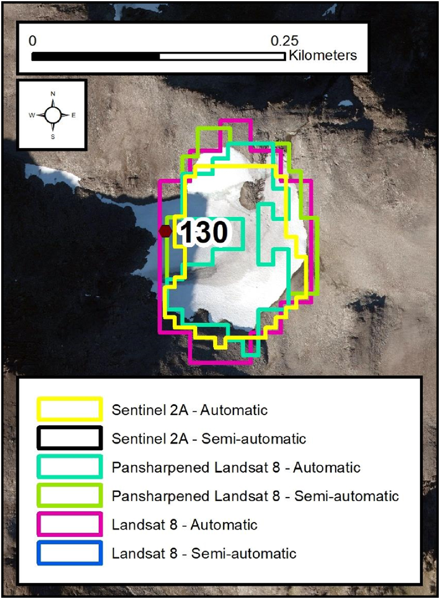
Overall, these results indicate that it is difficult to consistently and objectively map very small glaciers in the study area using both the automatic and semi-automatic approaches. Increasing image resolution (from 30 to 10 m) reduced variance in the mapping of the large glaciers (Fig. 5), but there was increased variance and uncertainty when mapping very small glaciers (Fig. 6). Furthermore, there was an inverse relationship between image resolution and the total mapped area for both semi-automatic and automatic approaches; more glacier units are mapped on the higher resolution imagery (10 and 15 m) than on the coarse-resolution imagery (30 m) yet, the cumulative mapped area of these units is lower (Table 3). Minimum size-thresholds will obviously reduce the total number of units mapped (sometimes by >90%) and can result in a substantial decrease in the total mapped area (Table 3). Higher resolution (⩽10 m) imagery may show that implementing minimum size-thresholds leads to the erroneous removal of genuine glaciers, as in Figure 6.
4.1.2. Manual mapping
Mapping glaciers manually is more subjective and arguably less consistent than the automated and semi-automated techniques described above. Our results show different glacier outlines from the different users, confirming previous work conducting ‘round-robin’ experiments with glacier mapping (e.g. Paul and others, Reference Paul2015). On the Landsat 8 imagery (30 m), there were major differences in both the total area and number of glaciers mapped. For example, Users 2 and 3 mapped fewer glaciers (37 and 16, respectively) than User 1, but User 3 mapped the largest cumulative glacier area (Table 3). However, manual mapping resulted in the least amount of difference in the number of mapped units between different image resolutions. In almost all cases, manual mapping reduces the number of units mapped compared with the automated, and semi-automated techniques (Table 3). Similar results were also found by Fischer and others (Reference Fischer, Huss, Barboux and Hoelzle2014).
When comparing image resolution and individual unit sizes, it is the largest units that experience the greatest absolute differences in mapped size, yet smaller percentage differences. The largest glacier unit manually mapped by each user on the 30 m resolution imagery (2.5818, 2.3480 and 2.1292 km2) shows a maximum difference of ~0.45 km2 or ~19% (Table 3). In contrast, the smallest unit manually mapped by each user on the 30 m resolution imagery (0.0377, 0.00243 and 0.0160 km2) shows a maximum difference of only ~0.02 km2 yet this equates to ~81% (Table 3). Manual mapping on the 15 and 10 m resolution imagery resulted in a maximum unit size of ~2.18 and 2.13 km2, respectively, while the minimum unit size was ~0.02 km2. At resolutions from 30 to 10 m, individual users were able to identify and map glaciers <0.05 km2. However, no units smaller than <0.01 km2 were manually mapped, suggesting that there is a lower size limit for confidently identifying glaciers on coarse (30 m) to medium (10 m) resolution imagery.
4.2. Aerial orthophotographs; manual mapping
When comparing the manual mapping on high-resolution imagery (aerial orthophotographs, <1 m) against coarse-resolution imagery (Landsat 8 imagery 30 m), it is clear that image resolution affects what is perceived and subsequently mapped as a glacier, especially with regards to the smallest glacier units. While two out of three users mapped more glaciers on coarse (30 m) compared to high-resolution (<1 m) imagery, all three users mapped a smaller total glacier area on the high-resolution imagery (Table 3). Again similar results were also found by Fischer and others (Reference Fischer, Huss, Barboux and Hoelzle2014). When image resolution is increased from 30 m (Landsat 8 imagery) to 0.25 m (aerial orthophotographs), the largest total area mapped decreases from 12.94 to 9.52 km2 (a 26% reduction) (Table 3). The higher resolution also resulted in smaller units being mapped, the smallest unit decreased from 0.016 km2 on the Landsat 8 imagery to 0.0004 km2 on the aerial orthophotographs (a 98% reduction; Table 3). The maximum difference between users for the total mapped area is only 0.95 km2 on the aerial orthophotographs, as opposed to 2.72 km2 on the Landsat 8 imagery (Table 3). This lower total variation on the orthophotographs is caused by lower variation in the mapping of larger glaciers.
When manual mapping using high-resolution aerial orthophotographs, the number of glacier units mapped ranged from 53 to 117, while the total glaciated area ranged from 8.57 to 9.52 km2 (Table 3). However, it should be noted that the user who identified the highest number of units did not map the largest cumulative glacier area. This is because 51 of the 117 units mapped (44%) were <0.01 km2 in area and the areas of both the largest units (glaciers 157 and 158) are smaller, resulting in a low cumulative glacier area. The minimum glacier size ranges from 0.0004 to 0.0171 km2 while the maximum glacier size ranges from 1.8266 to 1.9995 km2 (Table 3). These results highlight the fact that when manually mapping glaciers on the aerial orthophotographs (<1 m), all operators were able to map very small glaciers, with two out of three users mapping units <0.01 km2 (Table 3).
All users mapped a greater number of glaciers on the aerial orthophotographs than were in the NGI. However, the total area of glaciers has decreased, in part because the aerial orthophotographs are from a more recent date and some glaciers have retreated. Indeed, there are eight examples whereby glacier fragmentation has resulted in more units mapped (e.g. Fig. 7). Glacier fragmentation, therefore, accounts for a 30, 16 and 12% increase in the number of glaciers mapped by Users 1, 2 and 3, respectively.
Glacier 151 has fragmented over time. It has been mapped as multiple units by Users 1 and 2, while User 3 has mapped only one portion of the glacier. The grey outline shows the extent of glacier 151 from the NGI, mapped in 2001 from Landsat 7 imagery. Background image: natural colour aerial orthophotograph (0.25 m resolution). Location shown in Figure 1.
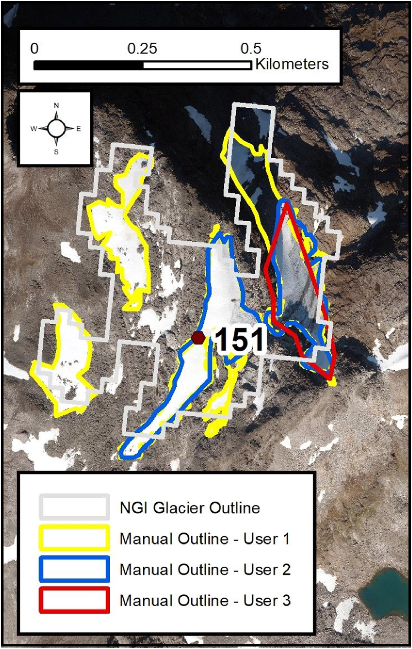
To summarise, the results show that increasing image resolution increased the number of glaciers that can be identified and mapped. Furthermore, on the high-resolution imagery (<1 m), it was possible for users to map numerous very small glaciers with individual extents <0.01 km2 (Table 3). The mapping of units <0.01 km2 by users is attributed to the fact they were able to define specific glacier surface features (e.g. glacier ice, evidence of flow at the surface of the ice) which helped to differentiate glacier units from snowpatches. However, for the smallest units mapped (specifically those <0.01 km2), there was an increase in differences between users as to what is identified and mapped as a glacier on the high-resolution imagery (<1 m), compared to the lower resolution imagery (30–15 m).
5. Discussion and recommendations for future work
There is a large body of literature on the best practice for mapping glaciers >1 km2 using satellite imagery (e.g. Raup and others, Reference Raup2007; Paul and others, Reference Paul2009, Reference Paul2013; Racoviteanu and others, Reference Racoviteanu, Paul, Raup, Khalsa and Armstrong2009), but there is little guidance on identifying and mapping very small glaciers (<0.5 km2), which are often ignored on medium to coarse-resolution imagery. This lack of guidance can be problematic given the burgeoning availability of high-resolution satellite imagery and aerial photographs, from which we can now identify these very small glaciers. From the analysis above, it is clear that the resolution of the imagery used, and the techniques applied have a substantial impact on the mapped glacial area that results. This is further influenced by the knowledge and experience of the operator, and the methods applied to define a glacier, particularly for glaciers <0.5 km2. The following sections present a discussion and offer subsequent guidelines to aid in the identification and mapping of very small glaciers.
5.1. Mapping approaches on coarse- to medium-resolution imagery (30, 15 and 10 m)
Regardless of image resolution, automated techniques often fail to map the full extent of many units (when compared to high-resolution aerial photographs). This is attributed to the inherent problems with automated glacier mapping, typically arising from debris cover, pro-glacial lakes, shadow, remnant snow, ice boundary conditions and recently deglaciated terrain (Racoviteanu and others, Reference Racoviteanu, Paul, Raup, Khalsa and Armstrong2009). As such, errors in mapping often require manual correction.
When using the automated and semi-automated approaches, at 30–15 m pixel resolutions, there are very large uncertainties in both the number and total area of glaciers <0.01 km2. At 15–10 m pixel resolutions especially, maps were overcomplicated by noise from erroneous sources (e.g. late-lying snow). Due to uncertainty in mapping units <0.01 km2, minimum glacier size-thresholds were applied to the 30, 15 and 10 m resolution imagery. The results presented here clearly show that, even at the 30 m resolution, it is possible to identify glacier units <0.05 km2, including those in heavily shaded locations (e.g. Fig. 4). Such glaciers can be identified based on their basic form and geographical situation (e.g. distinct snow/ice visible, situated in a cirque, evidence of prior valley glaciation). A minimum size-threshold of 0.05 km2 may therefore be too large, as it is possible to identify glaciers <0.05 km2. However, it is difficult to identify glaciers <0.01 km2, confirming the need for a minimum size-threshold. On the coarse and medium resolution imagery, relative uncertainty in glacier outlines increases with decreasing glacier size (Fischer and others, Reference Fischer, Huss, Barboux and Hoelzle2014; Winsvold and others, Reference Winsvold, Andreassen and Kienholz2014), but there is still a need for the assessment of mapped features falling just below a size-threshold before their removal. Manual correction (e.g. for areas in cast shadow), as shown in Figure 8, may increase a glacier's area above a specific threshold and ensure it is included in the subsequent analysis (Paul and others, Reference Paul, Winsvold, Kääb, Nagler and Schwaizer2016).
Manually editing the Sentinel-2A imagery automated outlines (yellow outline) of glacier 142 allows all three individual units (with areas of 0.0029, 0.0005 and 0.0077 km2) to be identified and mapped as one connected unit (purple outline). Without manual rectification, the 0.05 and 0.01 km2 size-thresholds remove the automatically mapped glacier units. Background image: Sentinel-2A imagery (10 m resolution, R-G-B as 5-4-3). Location shown in Figure 1.
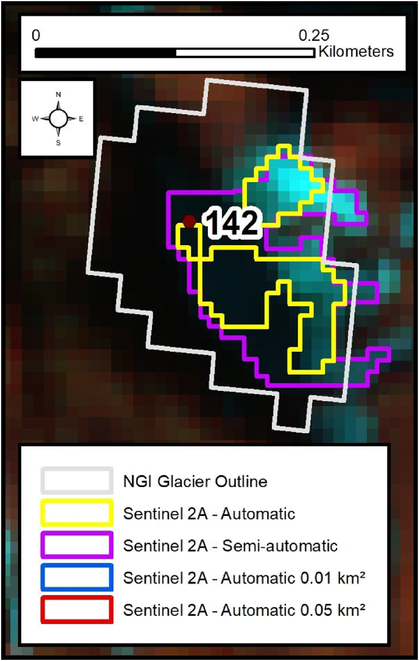
Furthermore, when comparing results from manual mapping on the Landsat 8 imagery (30 m), there is a large variation in the number and subsequent area of glaciers mapped. No user in this study mapped any units smaller than 0.01 km2, the smallest glaciers mapped ranged in size from ~0.02 to ~0.04 km2 (Table 3).
Given the above considerations, we confirm the current literature recommending that mapping on coarse to medium resolution imagery (30–10 m) uses a semi-automated approach with a 0.01 km2 minimum size-threshold, as per the GLIMS guidelines (Paul and others, Reference Paul2010).
5.2. Mapping approaches on high-resolution imagery (<1 m)
When mapping on the aerial orthophotographs, the application of a minimum glacier size-threshold seems unnecessarily cautious, as the higher resolution enables a clear definition of features attributable to a glacier (Fischer and others, Reference Fischer, Huss, Barboux and Hoelzle2014). An example of this is found in Figure 9, which shows a glacier mapped by all three operators. However, as shown in Table 3, large discrepancies remain in the number of units mapped as glaciers by different operators. This difference is again attributed to the increased level of subjectivity as a result of improved image resolution, especially with regards to distinguishing a snowpatch from a glacier.
(a) Location of an additional glacier (previously unmapped in the NGI) that all users mapped on aerial photographs in (b) but not on the Landsat 8 imagery (30 m resolution, R-G-B as 5-4-3) or Sentinel-2A imagery (10 m resolution, R-G-B as 5-4-3) in (c and d), respectively. When the scoring system is used, all users mapped this unit as certain. This unit is situated in a heavily shaded cirque, bordering a proglacial lake, and with a small amount of debris cover, all factors that hinder mapping on coarse-resolution multi-spectral imagery.
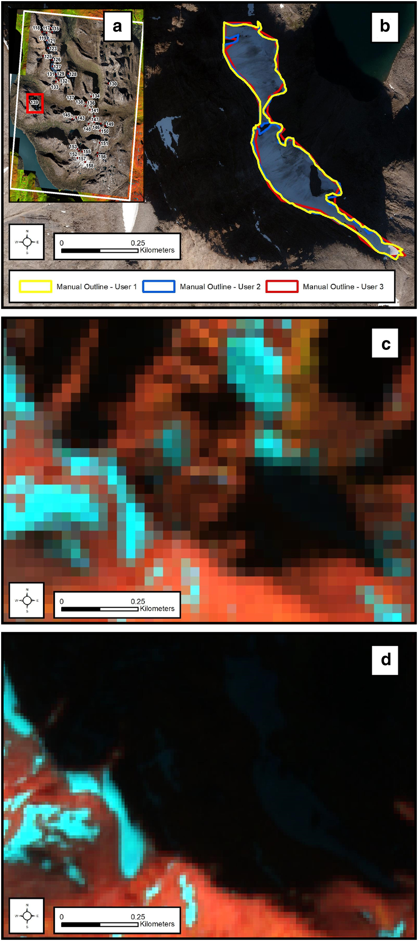
A significant point of note is that when mapping on the orthophotographs (<1 m resolution), multiple glaciers with an areal extent <0.01 km2 were mapped by two out of the three users. Furthermore, as glaciers of varying sizes (plateau, valley, cirque glaciers, etc.) continue to shrink and fragment under a warming climate, it is important that glacier inventories map all parts of a previously mapped glacier and do not ignore those falling below a certain size. Our results suggest that implementing a minimum size-threshold (even of 0.01 km2) on the imagery of <1 m resolution is inappropriate. We now address this issue by developing some criteria to aid the identification of glaciers on high-resolution imagery.
5.3. Identifying very small glaciers: a new scoring system
As demonstrated above, a lack of guidance on how to distinguish very small glaciers from snowpatches, when mapping from high-resolution remotely sensed imagery, resulted in a significant disparity between results from different mappers. This has been previously highlighted by the GLIMS project, where it was stated that ‘the methodological interpretation of a glacier as an entity varies widely, prompting the need for standardized methods’ (Racoviteanu and others, Reference Racoviteanu, Paul, Raup, Khalsa and Armstrong2009, p. 54). To our knowledge, no such standardised methods have so far been developed. We therefore propose a new scoring system to increase objectivity when identifying very small glaciers on high-resolution imagery (see Table 4). Our scoring system aims to reduce uncertainty and enable more robust and reliable glacier mapping, where image resolution and snow cover conditions permit. The system builds on and extends previous work by Evans (Reference Evans1990), who identified small glaciers in British Colombia based on three key indicators: crevasses, bergschrunds and (visible) ice. Furthermore, our scoring system incorporates the glacier definition of Cogley and others (Reference Cogley2011) whereby identification and subsequent glacier classification is weighted towards evidence of past and/or present flow.
Glacier identification scoring system for use in high-resolution (e.g. <1 m) remote-sensing applications
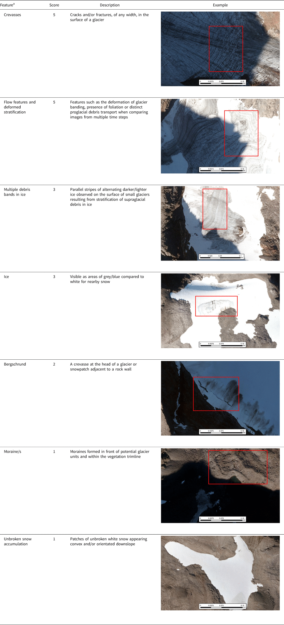
Summing the feature scores provides degree of confidence in identification as a glacier: 11–20 = certain; 6–10 = probable; 2–5 = possible; 1 = perennial snow. Images from 2016 source: https://www.norgeibilder.no/.
a These features are not visible on coarse (30–15 m) or medium (10 m) resolution imagery.
The new scoring system is based upon the examination of each potential glacier unit for specific features; it can be used with a single image but is best when used in conjunction with multiple images from differing years (if available), to confirm that features persist and to allow assessment under different snow cover conditions. This is of particular importance for very small glaciers which can experience ‘accumulation years’ and ‘ablation years’. In the former case, snow cover on the ice surface may obscure the ice and any flow features (e.g. deformation of debris banding), thereby giving a different score than if the feature was partially or totally snow free, as it would appear in the latter. Each candidate glacier is scored based on the features visible on the imagery (Table 4) and the resultant total score is used to classify the feature as either a ‘certain’, ‘probable’ or ‘possible’ glacier. A total score of 20 ‘points’ is possible depending on the number of specific visible features available. Initially just ice features were included but, on review, inclusion of moraines and snow was considered necessary. Together snow and moraines may reinforce other evidence of glacier presence in helping to inform decisions. Various value systems were tested, but the use of a possible maximum of 20 ‘points’ was considered optimal, as limiting the total score and associated feature values have kept the system simple and efficient.
We recognise four levels of evidence reliability. The clearest evidence of flowing ice is a set of crevasses, or deformation of banding lines and so each of these is awarded 5 points. Un-deformed parallel banding, from stratification of debris-rich versus debris-poor ice, indicates persistence and probably flow and receives 3 points, as does exposed uniform ice. A bergschrund is a single crevasse indicating consolidation or movement away from a headwall, so it does not rate as highly as a set of crevasses and is given 2 points. A moraine indicates that a glacier has been present and may or may not have survived, so it is ancillary evidence and awarded only a single point. Late-summer snow is a normal companion of glacier presence, but this might also be a snowpatch without flowing glacier ice. Snow, therefore, is given a single point. Convexity of a snowpatch has been suggested to indicate a greater likelihood that it hides a glacier (Groom, Reference Groom1959; Gachev and others, Reference Gachev, Stoyanov and Gikov2016), but under a warming climate, many glaciers are downwasting and thinning with a flattening of their surface. Therefore, lack of convexity of a snowpatch does not remove the possibility of buried glacier ice. However, consideration should be made of the incorrect interpretation of snow and associated moraine-like ridges, as it is possible they are periglacial features such as pronival ramparts (Hedding, Reference Hedding2016a). Pronival ramparts form at the base of perennial snowpatches and are not glacial in origin (Shakesby, Reference Shakesby1997; Hedding and Sumner, Reference Hedding and Sumner2013; Hedding, Reference Hedding2016b). Thus, there is a greater uncertainty where only ‘snow and moraines’ are visible and as such this uncertainty should be noted in any related attributes.
Where a score of 2–5 was obtained, the unit should be mapped and classified as only a possible glacier and should be marked for review when new imagery is available, or when it can be ground-truthed. A score from 6 to 10 means the unit should be mapped and classified as a probable glacier, again marked for future review. Finally, any unit scoring from 11 to 20 should be mapped as a certain glacier. These criteria are relevant irrespective of size. If the unit scores <2, it may be categorised as snow, or perennial snow if it occurs on multiple images. It can be important to record perennial snowpatches because they contribute not only to the hydrological regime, but can also influence carbon exchange and surface albedo (Zhang, Reference Zhang2005; Woo and Young, Reference Woo and Young2014; Medeiros and others, Reference Medeiros, Wood, Wesche, Bakaic and Peters2017; Young and others, Reference Young, Brown and Labine2018). Our approach offers a consistent and easily-applicable system, which should facilitate direct comparison between surveys conducted at different times and/or by different users. Thus, it is hoped that it will improve our ability to identify and monitor very small glaciers.
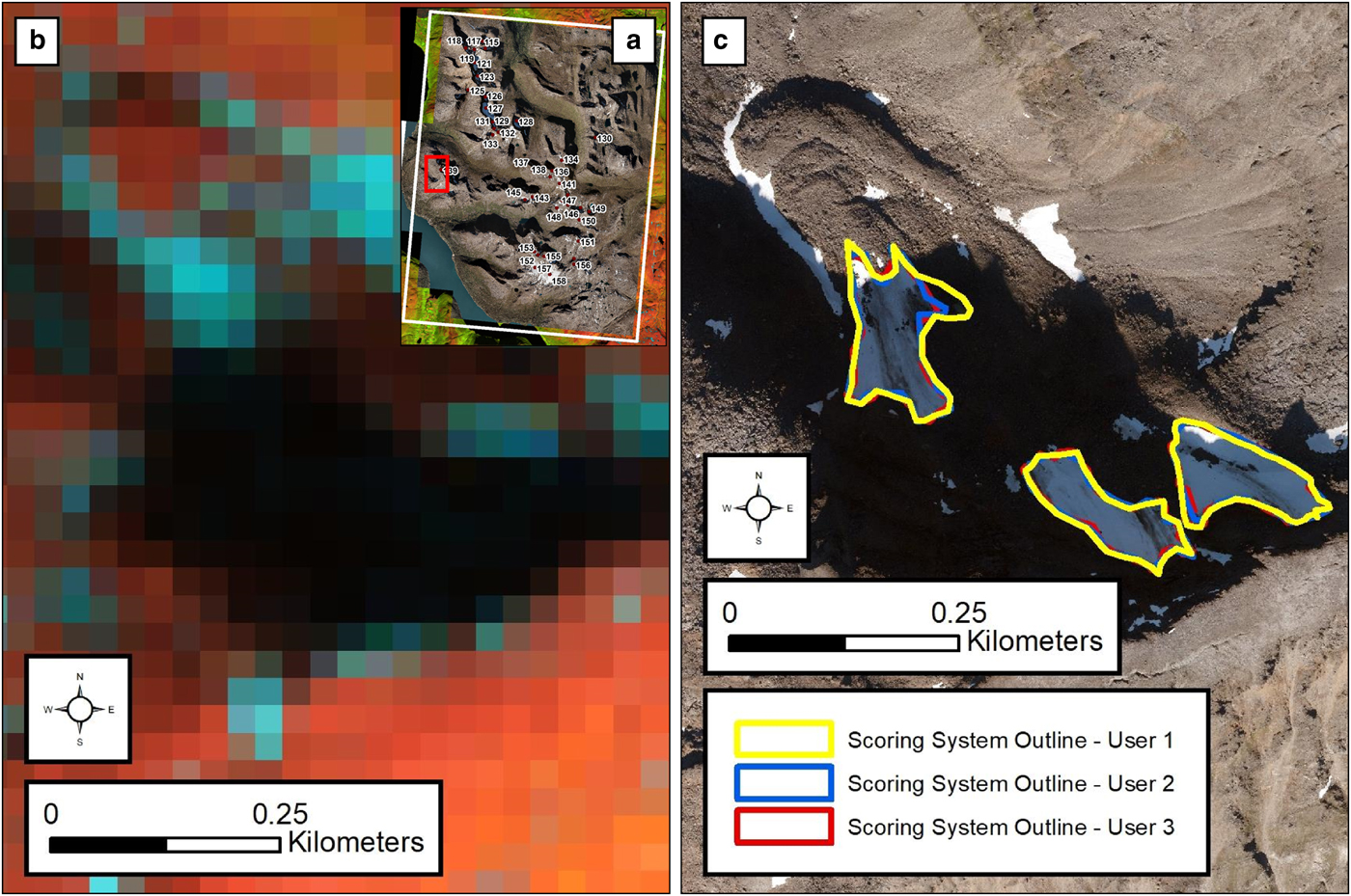
To test our scoring system, we conducted an additional mapping analysis following the criteria laid out in Table 4. As a result, there was a considerable reduction in variance between users when mapping glaciers that are classified as certain (Table 5). Without the scoring system, all mapped glaciers are, effectively, classed as certain, as there is no scope for classification based on degrees of certainty. Application of the scoring system reduced between-user differences in the total number of glaciers mapped by up to ~80% (Table 5). The maximum difference in mean glacier size between users also decreased by ~45% compared to the difference when glaciers were mapped without guidance. However, we note that some variability remains, and this occurs mainly in areas where heavy shading obscures the glacier surface, making it difficult to define surface features, or where remnant snow cover obscures glacier boundaries. Indeed, heavy shading and/or thin debris cover on snow can change its appearance, making it harder to make a definitive classification of snow versus ice. As a result, there is a greater variation in the number of possible and probable glaciers mapped, with some users still mapping more glacier units with these levels of uncertainty. In the case of heavy shading, methods for ‘de-shadowing’ previously employed on multispectral imagery (Richter and Müller, Reference Richter and Müller2005) show potential for use on true colour (RGB) aerial imagery, although these methods still require further research (Shahtahmassebi and others, Reference Shahtahmassebi, Yang, Wang, Moore and Shen2013; Movia and others, Reference Movia, Beinat and Crosilla2016). In the case of snow cover, to maximise accuracy, it is important to select images with minimum seasonal snow cover. Even if users are now able to map more glaciers, sub-optimal snow conditions may still lead to uncertainty regarding the exact extent of the glacier area. An example of glaciers that are consistently mapped by all three users, as a direct result of implementing the scoring system, is shown in Figure 10. Here, users were able to define glacial boundaries, even in challenging environments, where a high debris cover possibly obscures a large proportion of glacial ice. In this example (Fig. 10), all users limited their mapping to the exposed snow/ice, as it is unknown to what extent (if at all) ice exists beneath the debris. Due to this uncertainty in ice content of debris-covered areas, extrapolation beyond what is visible should be avoided to minimise uncertainty.
Number and area of glacier units digitised from aerial orthophotographs without the scoring system (see also Table 3) and after the implementation of the glacier identification scoring system

Showing how the scoring system reduces the number of certain glaciers mapped by each user and greatly increases the consistency between users, although there remains some variability, especially for possible glaciers.
An example of a particularly challenging unit (due to both debris cover and shade) that is only mapped by all three operators when following the scoring system on aerial orthophotographs. (a) Location of the previously unmapped units. (b) Landsat 8 image (30 m resolution, R-G-B as 5-4-3) showing a small area of ice/snow as blue yet a large area lies under heavy shadow. (c) Natural colour aerial orthophotograph (0.25 m resolution) showing the same area at the same scale, yet the ice/snow unit is easily mapped, even in heavy shadow. Debris surrounding the units means that they are mapped individually, although it is possible they are all connected. This example also shows how user subjectivity still affects scores: as User 1 mapped all units as possible, User 2 mapped all units as certain and User 3 mapped two as probable and one as possible.
A factor that cannot be resolved as a result of image adjustment and/or image acquisition dates is that of extensive/total supraglacial debris cover. In areas where glacial ice is entirely covered by debris, it is simply not possible to accurately define the unit extent and our scoring system is only applicable to debris-free areas (e.g. Fig. 10). Previous research has shown that mapping the extent of debris-covered glaciers can be very difficult, as the debris has very similar characteristics to the surrounding hillslopes from which it was sourced and debris inputs at the margins can make any break in slope between the ice surface and the hillslope difficult to identify (Paul and others, Reference Paul2013, Reference Paul2015). Furthermore, debris cover can obscure any ice and/or related flow features used in our classification and remotely sensed data cannot provide information on the internal ice content (Bhambri and others, Reference Bhambri, Bolch and Chaujar2011; Bhardwaj and others, Reference Bhardwaj2014; Lippl and others, Reference Lippl, Vijay and Braun2018). Indeed remote sensing generally fails to provide information about the internal ice content or structure of the unit in these situations, and so in situ observations would be needed to resolve uncertainty (Whalley and others, Reference Whalley, Martin and Gellatly1986; Bosson and Lambiel, Reference Bosson and Lambiel2016; Capt and others, Reference Capt, Bosson, Fischer, Micheletti and Lambiel2016). Additionally, meltwater streams may be identifiable at the terminus of some debris-covered glaciers and may provide an indication of buried glacier ice as opposed to an ice–rock mixture associated with permafrost features (Whalley and others, Reference Whalley, Martin and Gellatly1986). The issue of extensive/total debris cover is also relevant to the debate regarding the origin/formation of rock glaciers (Berthling, Reference Berthling2011), whereby similar looking features may have been formed as the result of different geomorphological processes (Martin and Whalley, Reference Martin and Whalley1987). Given the additional complexity and large uncertainties associated with mapping extensively debris-covered glaciers from remotely sensed imagery, the use of our new scoring system is restricted to largely non-debris-covered glaciers. However, establishing guidelines for the identification and mapping of largely debris-covered and rock glaciers may be possible in the future, building on work such as Charbonneau and Smith (Reference Charbonneau and Smith2018), who used Google Earth imagery to produce an inventory of rock glaciers in the central British Columbia Coast Mountains, Canada.
Overall, the system allows users to rank units according to specific features and therefore classify glaciers with degrees of certainty, which increases the information on ice bodies within the study area and provides a more objective, repeatable and consistent approach. It is, however, acknowledged that possible difficulties in the acquisition of high-resolution imagery and limitations of time available for inventory production can inhibit mapping of glaciers with exceedingly high levels of detail. In such instances, the proposed scoring system may instead be used as a means of validating mapping conducted on satellite imagery, thus providing an objective means of deciding if a unit should or should not be included in a glacier map.
6. Conclusions
In this paper, we compared how both image resolution and different techniques can influence the mapping of very small glaciers in northern Norway. With 30–15 m pixel resolution imagery, classification errors are prevalent within all methods. It is often not possible to define specific surface features indicative of glacier formation on individual snow/ice units <0.01 km2. This supports previous work (e.g. Paul and others, Reference Paul2010) recommending a minimum size-threshold of 0.01 km2 on the imagery of medium to coarse resolution. With increasing image resolution, errors can be mitigated with thorough and systematic assessment of individually mapped units (e.g. reviewing potential glacier units for specific glacial features or manually editing areas erroneously mapped). At 10 m pixel resolution, it is possible to define some individual features characteristic of glaciers, such as crevasses and small terminal moraines. Nonetheless, a minimum size-threshold of 0.01 km2 is advisable, as it is not possible to identify detailed features on smaller units. On imagery with pixel resolution <1 m, ice/snow units of all sizes can more easily be distinguished even in heavy shading. In this paper, multiple operators were able to map glaciers smaller than 0.01 km2 on aerial orthophotographs (0.25 m), indicating that a minimum size is inappropriate on high-resolution imagery. However, there are few published guidelines for identifying glaciers on high-resolution imagery. As a result, we have developed a new scoring system that classifies very small glaciers as certain, probable or possible. This is based on detailed ice surface structures (e.g. evidence of flow banding and crevasses) and diagnostic glacial landforms, such as moraines (Table 4). This scoring system provides a useful framework to increase the objective mapping of very small glaciers and reduce uncertainties in the next generation of glacier inventories using high-resolution imagery.
Acknowledgements
Landsat 8 OLI and Sentinel-2A imagery were downloaded free of charge from the USGS Earth Explorer website (https://earthexplorer.usgs.gov/) and aerial orthophotographs were kindly provided by the Norwegian Mapping Authority. Prior glacier data as collated by the CryoClim project were also used including glacier outlines downloaded from the NVE website (https://www.nve.no/hydrology/glaciers/glacier-data/). Joshua R. Leigh is supported by the Natural Environment Research Council UK studentship, reference: NE/L002590/1. This work will also act as a contribution to the project Copernicus bretjeneste (Copernicus Glacier Service Norway, Contract NIT.06.15.5). We are grateful for the encouraging comments from the late Graham Cogley during the inception of this manuscript. Finally, we thank the Editor (Christoph Schneider) and the diligent reviews provided by Mauro Fischer and an anonymous reviewer.


 Open access

