


1 Introduction
Descriptive set theory and computability theory study hierarchies of classes, that at first appear merely analogues, but in fact can be considered as manifestations of the same basic concept in different settings. The most prominent example is the Borel hierarchy of $\boldsymbol {\Sigma }^0_\alpha $
subsets of Polish spaces (for all countable ordinals
$\boldsymbol {\Sigma }^0_\alpha $
subsets of Polish spaces (for all countable ordinals $\alpha $
), and the hyperarithmetic hierarchy of
$\alpha $
), and the hyperarithmetic hierarchy of $\Sigma ^0_\alpha $
subsets of
$\Sigma ^0_\alpha $
subsets of $\mathbb N$
(for all computable ordinals
$\mathbb N$
(for all computable ordinals $\alpha $
). The underlying connection here is that the lightface (effective) classes
$\alpha $
). The underlying connection here is that the lightface (effective) classes $\Sigma ^0_\alpha $
can be defined not only for
$\Sigma ^0_\alpha $
can be defined not only for $\mathbb N$
, but also for subsets of any computably presented Polish space. They can be relativised to oracles z (and z-computable ordinals
$\mathbb N$
, but also for subsets of any computably presented Polish space. They can be relativised to oracles z (and z-computable ordinals $\alpha $
). We then get
$\alpha $
). We then get $\boldsymbol {\Sigma }^0_\alpha = \bigcup \left \{ \Sigma ^0_\alpha (z) \,:\, \alpha \text { is } z\text {-computable} \right \}$
. This enables us to apply effective methods to study Borel sets. Among prominent results in the effective theory, or using effective methods, are Louveau’s separation theorem [Reference Louveau12], the Harrington–Kechris–Louveau dichotomy [Reference Harrington, Kechris and Louveau10], and the
$\boldsymbol {\Sigma }^0_\alpha = \bigcup \left \{ \Sigma ^0_\alpha (z) \,:\, \alpha \text { is } z\text {-computable} \right \}$
. This enables us to apply effective methods to study Borel sets. Among prominent results in the effective theory, or using effective methods, are Louveau’s separation theorem [Reference Louveau12], the Harrington–Kechris–Louveau dichotomy [Reference Harrington, Kechris and Louveau10], and the $G_0$
-dichotomy [Reference Kechris, Solecki and Todorcevic11].
$G_0$
-dichotomy [Reference Kechris, Solecki and Todorcevic11].
A hierarchy finer than the Borel/hyperarithmetic one is defined using differences of sets in the Borel hierarchy. In set theory this is known as the Hausdorff, or Lavrentiev, difference hierarchy $D_\eta (\boldsymbol {\Sigma }^0_\alpha )$
. In computability, this is the Ershov hierarchy [Reference Ershov5–Reference Ershov6] (see also [Reference Putnam16]). The prominent result regarding the difference hierarchy in set theory is the Hausdorff–Kuratowski theorem, that
$D_\eta (\boldsymbol {\Sigma }^0_\alpha )$
. In computability, this is the Ershov hierarchy [Reference Ershov5–Reference Ershov6] (see also [Reference Putnam16]). The prominent result regarding the difference hierarchy in set theory is the Hausdorff–Kuratowski theorem, that $\boldsymbol {\Delta }^0_{\alpha +1}= \bigcup _{\eta <\omega _1}D_\eta (\boldsymbol {\Sigma }^0_\alpha )$
. The analogous result, due to Ershov, is that every
$\boldsymbol {\Delta }^0_{\alpha +1}= \bigcup _{\eta <\omega _1}D_\eta (\boldsymbol {\Sigma }^0_\alpha )$
. The analogous result, due to Ershov, is that every $\Delta ^0_2$
set is
$\Delta ^0_2$
set is $\Sigma ^{-1}_\eta $
for some notation
$\Sigma ^{-1}_\eta $
for some notation $\eta $
for a computable ordinal (
$\eta $
for a computable ordinal ( $\Sigma ^{-1}_\eta $
is Ershov’s notation for
$\Sigma ^{-1}_\eta $
is Ershov’s notation for $D_\eta (\Sigma ^0_1)$
). The effective version is more “fragile,” as the class
$D_\eta (\Sigma ^0_1)$
). The effective version is more “fragile,” as the class $D_\eta (\Sigma ^0_1)$
depends on the notation (computable presentation) of
$D_\eta (\Sigma ^0_1)$
depends on the notation (computable presentation) of $\eta $
, rather than just its order-type.
$\eta $
, rather than just its order-type.
The finest hierarchy of them all is due to Wadge [Reference Wadge25]. Motivated by “many-one” reducibility in computability, Wadge defined a subset A of Baire space to be reducible to B if A is a continuous pre-image of B. A Wadge class is a collection of sets closed under taking continuous pre-images. The structure of Borel Wadge classes under containment is surprisingly regular; it is semi-well-ordered, with alternating self-dual and non-self-dual classes. Wadge was able to calculate the order-type of the non-self-dual classes (after identifying such a class with its dual). He also showed that all such classes are the result of applying a Borel $\omega $
-ary Boolean operation to the class of open sets.
$\omega $
-ary Boolean operation to the class of open sets.
In computability, the analogue of the Wadge hierarchy was defined by Selivanov [Reference Selivanov19, Reference Selivanov20], which he called the fine hierarchy. To avoid the problem of dependence on ordinal notation, Selivanov looked at generalisations of the finite difference hierarchy. The hierarchy was first defined using generalised jump operations in [Reference Selivanov19]. This resembles Wadge’s use of Kuratowski $(\mu ,0)$
-homeomorphisms, which we now know can be thought of as relativised iterated Turing jumps. In [Reference Selivanov20], Selivanov gave an inductive definition of the hierarchy (of length
$(\mu ,0)$
-homeomorphisms, which we now know can be thought of as relativised iterated Turing jumps. In [Reference Selivanov20], Selivanov gave an inductive definition of the hierarchy (of length $\varepsilon _0$
), using (essentially) jumps, and some fixed Boolean operations, most notably the BiSep operation (two sided separated unions). In [Reference Selivanov21], an equivalent definition is given using typed Boolean terms. Selivanov also noted a close relationship between the fine hierarchy and the Wagner hierarchy in automata theory [Reference Selivanov22, Reference Wagner26]. For a survey, see [Reference Selivanov23]. Selivanov also generalised his hierarchy beyond subsets of spaces, to k-partitions and functions to BQOs [Reference Selivanov, Löwe, Normann, Soskov and Soskova17, Reference Selivanov18], and to general Polish and quasi-Polish spaces [Reference Selivanov24].
$\varepsilon _0$
), using (essentially) jumps, and some fixed Boolean operations, most notably the BiSep operation (two sided separated unions). In [Reference Selivanov21], an equivalent definition is given using typed Boolean terms. Selivanov also noted a close relationship between the fine hierarchy and the Wagner hierarchy in automata theory [Reference Selivanov22, Reference Wagner26]. For a survey, see [Reference Selivanov23]. Selivanov also generalised his hierarchy beyond subsets of spaces, to k-partitions and functions to BQOs [Reference Selivanov, Löwe, Normann, Soskov and Soskova17, Reference Selivanov18], and to general Polish and quasi-Polish spaces [Reference Selivanov24].
In this article, we show how to naturally extend Selivanov’s hierarchy beyond the arithmetic, all the way up the hyperarithmetic sets. To do this, we give a new way to define the hierarchy, using descriptions of Borel Wadge classes that were introduced in [Reference Day, Greenberg, Harrison-Trainor and Turetsky1] and systematically investigated in [Reference Greenberg and Turetsky9]. These are descriptions that generalise ones given by Louveau [Reference Louveau13] and by Louveau and Saint Raymond [Reference Louveau and Raymond14]. The levels of the extended hierarchy will be the ones that have finite descriptions.
We then give a game characterisation of containment between classes, which is a modification of one given for Borel Wadge classes in [Reference Greenberg and Turetsky9]. Using this characterisation we can explain why the fine hierarchy satisfies Wadge’s semi-linear ordering principle. Essentially, this is due to the determinacy of finite games. We also use this game characterisation to explain why the hierarchy is well-founded.
To calculate the height of a class in the fine hierarchy, we introduce the notion of an admissible description, and show that every class in the hierarchy has such a description. Admissible descriptions directly give us information about the class described, for example, if it is at a successor or limit level.
The class descriptions we introduce utilise Montalbán’s method of true stages (a non-effective version was introduced independently in [Reference Debs and Raymond3]). This allows us to computably approximate sets at all levels in the extended fine hierarchy: our descriptions are inherently dynamic. This is useful when performing priority arguments. In the sequel to this paper [Reference Greenberg, Qi and Turetsky7], we do exactly that, to give a complete answer to the question of which levels of the hierarchy contain new Turing degrees.
2 Preliminaries: Described classes
To define and analyse the classes of the extended fine hierarchy, we use the class descriptions introduced in [Reference Day, Greenberg, Harrison-Trainor and Turetsky1, Reference Greenberg and Turetsky9]. These are used to define classes of subsets of Baire space. We can, however, identify the natural numbers as a subspace of Baire space (identify n with the infinite sequence $n^\infty $
). To simplify notation we use true stage relations on
$n^\infty $
). To simplify notation we use true stage relations on $\omega +1$
rather than
$\omega +1$
rather than $\omega ^{\leqslant \omega }$
, that were developed in [Reference Greenberg and Turetsky8], and adapt the class descriptions to this setting.
$\omega ^{\leqslant \omega }$
, that were developed in [Reference Greenberg and Turetsky8], and adapt the class descriptions to this setting.
2.1 True stage relations
The true stage relations allow us to computably approximate transfinite iterations of the Turing jump.
A concrete computable ordinal is a computable well-ordering of a computable subset of $\mathbb N$
, in which the successor relation and collection of limit points are both computable. For concrete computable ordinals
$\mathbb N$
, in which the successor relation and collection of limit points are both computable. For concrete computable ordinals $\alpha $
and
$\alpha $
and $\beta $
we write
$\beta $
we write $\alpha <\beta $
if
$\alpha <\beta $
if $\alpha $
is an initial segment of
$\alpha $
is an initial segment of $\beta $
. For every concrete computable ordinal
$\beta $
. For every concrete computable ordinal $\alpha $
we obtain a partial ordering
$\alpha $
we obtain a partial ordering $\leqslant _\alpha $
on
$\leqslant _\alpha $
on $\omega +1$
with a variety of pleasing properties. In particular:
$\omega +1$
with a variety of pleasing properties. In particular:
-
(i) $\leqslant _0$
is the usual ordering
$\leqslant $
on
$\omega +1$
.
$\leqslant _0$
is the usual ordering
$\leqslant $
on
$\omega +1$
. -
(ii) If
$\alpha <\beta $
then
$s\leqslant _\beta t$
implies
$s\leqslant _\alpha t$
. -
(iii)
$(\omega +1,\leqslant _\alpha )$
is a tree, with root 0. -
(iv)
$\{s\,:\, s<_\alpha \omega \}$
is the unique infinite path of
$(\omega ,\leqslant _\alpha )$
. -
(v) The restriction of
$\leqslant _\alpha $
to
$\omega $
is computable, uniformly in
$\alpha $
. -
(vi) A set
$A\subseteq \mathbb N$
is
$\Sigma ^0_{1+\alpha }$
if and only if its characteristic function
$1_A$
has a computable
$\alpha $
-enumeration: a computable function
$f\colon \mathbb N\times \omega \to \{0,1\}$
satisfying, for all
$x\in \mathbb N$
:-
• If
$s\leqslant _\alpha t$
and
$f(x,s)=1$
then
$f(x,t)=1$
. -
•
$1_A(x) = \lim \{f(x,s)\,:\, s<_\alpha \omega \}$
.
-


In (vi), and below, we write $\mathbb N\times \omega $
(rather than
$\mathbb N\times \omega $
(rather than $\mathbb N^2$
) to indicate that the first input x is an element of the “space”
$\mathbb N^2$
) to indicate that the first input x is an element of the “space” $\mathbb N$
, and the second represents a stage of the approximation.
$\mathbb N$
, and the second represents a stage of the approximation.
For Propositions 2.1 and 2.3 below, recall that a function $h\colon \mathbb N\to \mathbb N$
is
$h\colon \mathbb N\to \mathbb N$
is $\Delta ^0_\alpha $
-measurable if for all n,
$\Delta ^0_\alpha $
-measurable if for all n, $h^{-1}[\{n\}]$
is
$h^{-1}[\{n\}]$
is $\Delta ^0_{\alpha }$
, uniformly in n. This is equivalent to being
$\Delta ^0_{\alpha }$
, uniformly in n. This is equivalent to being $\Sigma ^0_\alpha $
-measurable.
$\Sigma ^0_\alpha $
-measurable.
We will use the following corollary of property (vi).
Proposition 2.1. Let $\alpha $
be a concrete computable ordinal. Let
$\alpha $
be a concrete computable ordinal. Let $h\colon \mathbb N\to \mathbb N$
be
$h\colon \mathbb N\to \mathbb N$
be $\Delta ^0_{1+\alpha }$
-measurable. Then h admits an “
$\Delta ^0_{1+\alpha }$
-measurable. Then h admits an “ $\alpha $
-decision procedure”: a computable function
$\alpha $
-decision procedure”: a computable function $f\colon \mathbb N\times \omega \to \mathbb N\cup \{?\}$
satisfying:
$f\colon \mathbb N\times \omega \to \mathbb N\cup \{?\}$
satisfying:
-
• If
$s\leqslant _\alpha t$
and
$f(x,s)\in \mathbb N$
then
$f(x,t)= f(x,s)$
. -
• For all x, for all but finitely many
$s<_\alpha \omega $
,
$f(x,s) = h(x)$
.


That is, for a while, $f(x,s)$
could be ?, indicating that we are not yet sure what
$f(x,s)$
could be ?, indicating that we are not yet sure what $h(x)$
is; but once some value is guessed for
$h(x)$
is; but once some value is guessed for $h(x)$
, we never change our mind again. Along the
$h(x)$
, we never change our mind again. Along the $\alpha $
-true stages (the stages
$\alpha $
-true stages (the stages $s<_\alpha \omega $
), we eventually guess the correct value.
$s<_\alpha \omega $
), we eventually guess the correct value.
Proof. For each n, let $A_n = h^{-1}[\{n\}]$
. Let
$A_n = h^{-1}[\{n\}]$
. Let $g_n$
be uniformly computable
$g_n$
be uniformly computable $\alpha $
-enumerations of
$\alpha $
-enumerations of $A_n$
. Let
$A_n$
. Let $x\in \mathbb N$
. We define
$x\in \mathbb N$
. We define $f(x,s)$
by recursion on
$f(x,s)$
by recursion on $s<\omega $
. If there is some
$s<\omega $
. If there is some $r<_\alpha s$
such that
$r<_\alpha s$
such that $f(x,r)\in \mathbb N$
, then we let
$f(x,r)\in \mathbb N$
, then we let $f(x,s) = f(x,r)$
. Otherwise, if there is some
$f(x,s) = f(x,r)$
. Otherwise, if there is some $n\leqslant s$
such that
$n\leqslant s$
such that $g_n(x,s)=1$
then we let
$g_n(x,s)=1$
then we let $f(x,s)=n$
for the least such n. If there is no such n then we let
$f(x,s)=n$
for the least such n. If there is no such n then we let $f(x,s)=?$
.
$f(x,s)=?$
.
We remark that (vi) is uniform: given a $\Sigma ^0_{1+\alpha }$
index of A, we can effectively compute an
$\Sigma ^0_{1+\alpha }$
index of A, we can effectively compute an $\alpha $
-enumeration of A. As a result, Proposition 2.1 is also uniform: from a
$\alpha $
-enumeration of A. As a result, Proposition 2.1 is also uniform: from a $\Delta ^0_{1+\alpha }$
-index for the sets
$\Delta ^0_{1+\alpha }$
-index for the sets $h^{-1}(\{n\})$
, we can effectively compute a computable index of an
$h^{-1}(\{n\})$
, we can effectively compute a computable index of an $\alpha $
-decision procedure f.
$\alpha $
-decision procedure f.
Definition 2.2. A computable $\alpha $
-approximation is a function
$\alpha $
-approximation is a function $f\colon \mathbb N\times \omega \to \mathbb N$
such that for all x,
$f\colon \mathbb N\times \omega \to \mathbb N$
such that for all x, $\lim \left \{ f(x,s) \,:\, s<_\alpha \omega \right \}$
exists. The function approximated by f is the one taking x to that stable value.
$\lim \left \{ f(x,s) \,:\, s<_\alpha \omega \right \}$
exists. The function approximated by f is the one taking x to that stable value.
The following is a “higher limit lemma.” It is proved in [Reference Day, Greenberg, Harrison-Trainor and Turetsky2, Proposition 3.6].
Proposition 2.3. A function $g\colon \mathbb N\to \mathbb N$
has a computable
$g\colon \mathbb N\to \mathbb N$
has a computable $\alpha $
-approximation if and only if it is
$\alpha $
-approximation if and only if it is $\Delta ^0_{1+\alpha +1}$
-measurable.
$\Delta ^0_{1+\alpha +1}$
-measurable.
We will require a particular type of $\alpha $
-approximations, that generalises the notion of an
$\alpha $
-approximations, that generalises the notion of an $\alpha $
-enumeration. Let
$\alpha $
-enumeration. Let $n\geqslant 1$
. An
$n\geqslant 1$
. An $(\alpha ,n)$
-enumeration is an
$(\alpha ,n)$
-enumeration is an $\alpha $
-approximation f such that for all x,
$\alpha $
-approximation f such that for all x,
-
•
$f(x,0)=0$
; -
• for all s,
where
$$\begin{align*}\# \left\{ t\leqslant_{\alpha} s \,:\, f(x,t)\ne f(x,t^{-\alpha}) \right\} \leqslant n, \end{align*}$$
$t^{-\alpha }$
is t’s predecessor in the tree
$(\omega ,<_\alpha )$
.


An $(\alpha ,1)$
-enumeration is simply an
$(\alpha ,1)$
-enumeration is simply an $\alpha $
-enumeration (with the added requirement that
$\alpha $
-enumeration (with the added requirement that $f(x,0)=0$
, which is an easy modification).
$f(x,0)=0$
, which is an easy modification).
Proposition 2.4. A set has an $(\alpha ,n)$
-enumeration if and only if it is
$(\alpha ,n)$
-enumeration if and only if it is $D_n(\Sigma ^0_{1+\alpha })$
.
$D_n(\Sigma ^0_{1+\alpha })$
.
Proof. Suppose that C has an $(\alpha ,n)$
-enumeration f. For
$(\alpha ,n)$
-enumeration f. For $k\leqslant n$
let
$k\leqslant n$
let $A_k$
be the set of
$A_k$
be the set of $x\in \mathbb N$
such that there are
$x\in \mathbb N$
such that there are $s_0 <_{\alpha } s_1 <_\alpha s_2 <_\alpha \cdots <_\alpha s_k <_\alpha \omega $
such that
$s_0 <_{\alpha } s_1 <_\alpha s_2 <_\alpha \cdots <_\alpha s_k <_\alpha \omega $
such that $f(x,s_i)\ne f(x,s_{i+1})$
for all
$f(x,s_i)\ne f(x,s_{i+1})$
for all $i<k$
. Then each
$i<k$
. Then each $A_k$
is
$A_k$
is $\Sigma ^0_{1+\alpha }$
,
$\Sigma ^0_{1+\alpha }$
, $\mathbb N = A_0 \supseteq A_1 \supseteq A_2 \supseteq \cdots \supseteq A_n$
, and
$\mathbb N = A_0 \supseteq A_1 \supseteq A_2 \supseteq \cdots \supseteq A_n$
, and $C = (A_1\setminus A_2)\cup (A_3\setminus A_4)\cup \cdots $
, showing that C is
$C = (A_1\setminus A_2)\cup (A_3\setminus A_4)\cup \cdots $
, showing that C is $D_n(\Sigma ^0_{1+\alpha })$
. In the other direction, let
$D_n(\Sigma ^0_{1+\alpha })$
. In the other direction, let $C = (A_1\setminus A_2)\cup (A_3\setminus A_4)\cup \cdots $
, with
$C = (A_1\setminus A_2)\cup (A_3\setminus A_4)\cup \cdots $
, with $A_i\in \Sigma ^0_{1+\alpha }$
and
$A_i\in \Sigma ^0_{1+\alpha }$
and $A_1\supseteq A_2\supseteq \cdots \supseteq A_n$
. For
$A_1\supseteq A_2\supseteq \cdots \supseteq A_n$
. For $i=1,\dots , n$
, let
$i=1,\dots , n$
, let $g_i$
be an
$g_i$
be an $\alpha $
-enumeration of
$\alpha $
-enumeration of $A_i$
. For simplicity let
$A_i$
. For simplicity let $g_0(x,s)=1$
for all x and s. We may also assume that
$g_0(x,s)=1$
for all x and s. We may also assume that $g_i(x,s)=1$
implies
$g_i(x,s)=1$
implies $g_{i-1}(x,s)=1$
when
$g_{i-1}(x,s)=1$
when $i>0$
. We let
$i>0$
. We let $f(x,s)=0$
if the greatest i such that
$f(x,s)=0$
if the greatest i such that $g_i(x,s)=1$
is even,
$g_i(x,s)=1$
is even, $f(x,s)=1$
otherwise. Then f is an
$f(x,s)=1$
otherwise. Then f is an $(\alpha ,n)$
-enumeration of C.
$(\alpha ,n)$
-enumeration of C.
2.2 Class descriptions
A (computable) class description $\Gamma $
consists of a well-founded computable tree
$\Gamma $
consists of a well-founded computable tree $T_\Gamma \subset \omega ^{<\omega }$
, computably labelled as follows:
$T_\Gamma \subset \omega ^{<\omega }$
, computably labelled as follows:
-
(i) If
$\sigma \in T_\Gamma $
is not a leaf of
$T_\Gamma $
, then
$\sigma $
is labelled by a pair
$(\xi _\sigma ,\eta _\sigma )$
where
$\xi _\sigma $
and
$\eta _\sigma $
are concrete computable ordinals, and
$\eta _\sigma \geqslant 1$
. -
(ii) If
$\sigma \in T_\Gamma $
is a leaf of
$T_\Gamma $
then
$\sigma $
is labelled by a value
$\Gamma (\sigma )\in \{0,1\}$
.


We use the term internal node of a tree T to denote a node of T that is not a leaf of T. We require that if $\sigma \preccurlyeq \tau $
are both internal nodes of
$\sigma \preccurlyeq \tau $
are both internal nodes of $T_\Gamma $
then
$T_\Gamma $
then $\xi _\sigma \leqslant \xi _\tau $
. We let
$\xi _\sigma \leqslant \xi _\tau $
. We let $o(\Gamma ) = \xi _{{\left \langle {}\right \rangle }}$
be the
$o(\Gamma ) = \xi _{{\left \langle {}\right \rangle }}$
be the $\xi $
-label of the root
$\xi $
-label of the root ${\left \langle {}\right \rangle }$
of
${\left \langle {}\right \rangle }$
of $T_\Gamma $
, unless
$T_\Gamma $
, unless $T_\Gamma $
consists only of the root, in which case we set
$T_\Gamma $
consists only of the root, in which case we set $o(\Gamma )=\omega _1$
(where
$o(\Gamma )=\omega _1$
(where $\omega _1$
is treated as a formal symbol). We similarly set
$\omega _1$
is treated as a formal symbol). We similarly set $\xi _\sigma = \omega _1$
for a leaf
$\xi _\sigma = \omega _1$
for a leaf $\sigma $
of
$\sigma $
of $T_\Gamma $
. We let
$T_\Gamma $
. We let ![]() .
.
The idea is that at an internal node $\sigma $
we need to choose one of its children. The leftmost child is considered a default, the one we choose initially. We can change our mind about the child we are choosing, but the “number” of mind changes is bounded by
$\sigma $
we need to choose one of its children. The leftmost child is considered a default, the one we choose initially. We can change our mind about the child we are choosing, but the “number” of mind changes is bounded by $\eta _\sigma $
: every time we change our mind, we need to decrease the ordinal. The ordinal
$\eta _\sigma $
: every time we change our mind, we need to decrease the ordinal. The ordinal $\xi _\sigma $
tells us at what level we conduct this approximation. Informally, this means that the approximation is computable from
$\xi _\sigma $
tells us at what level we conduct this approximation. Informally, this means that the approximation is computable from $\emptyset ^{(\xi _\sigma )}$
. Technically, we use the true stage relations. Our intention is formalised using the notion of a
$\emptyset ^{(\xi _\sigma )}$
. Technically, we use the true stage relations. Our intention is formalised using the notion of a $\Gamma $
-name.
$\Gamma $
-name.
If $\Gamma $
is a computable class description, then a (computable)
$\Gamma $
is a computable class description, then a (computable) $\Gamma $
-name N consists of a choice, for each internal
$\Gamma $
-name N consists of a choice, for each internal $\sigma \in T_\Gamma $
, of a pair of functions
$\sigma \in T_\Gamma $
, of a pair of functions $(f_\sigma ,\beta _\sigma )$
, uniformly computable given
$(f_\sigma ,\beta _\sigma )$
, uniformly computable given $\sigma $
, both defined on
$\sigma $
, both defined on $\mathbb N\times \omega $
, satisfying the following:
$\mathbb N\times \omega $
, satisfying the following:
-
(i) For each
$(x,s)\in \mathbb N\times \omega $
,
$f_\sigma (x,s)$
is a child of
$\sigma $
on
$T_\Gamma $
, and
$\beta _\sigma (x,s) \leqslant \eta _\sigma $
. -
(ii) For each
$x\in \mathbb N$
and
$s,t\in \omega $
, if
$s\leqslant _{\xi _\sigma }t$
then:-
•
$\beta _\sigma (x,t)\leqslant \beta _\sigma (x,s)$
; -
• if
$f_\sigma (x,t)\ne f_\sigma (x,s)$
then
$\beta _\sigma (x,t)< \beta _\sigma (x,s)$
.
-
-
(iii) For each
$(x,s)\in \mathbb N\times \omega $
, if
$\beta _\sigma (x,s) = \eta _\sigma $
then
$f_\sigma (x,s)$
is the leftmost child of
$\sigma $
on
$T_\Gamma $
(the default outcome of
$\sigma $
).


Let N be a $\Gamma $
-name. The definition ensures that for all internal
$\Gamma $
-name. The definition ensures that for all internal $\sigma \in T_\Gamma $
, for all
$\sigma \in T_\Gamma $
, for all $x\in \mathbb N$
, the limit
$x\in \mathbb N$
, the limit $\lim \left \{ f_\sigma (x,s) \,:\, s<_{\xi _{\sigma }} \omega \right \}$
exists, and we denote it by
$\lim \left \{ f_\sigma (x,s) \,:\, s<_{\xi _{\sigma }} \omega \right \}$
exists, and we denote it by $f_\sigma (x)$
. Since
$f_\sigma (x)$
. Since $T_\Gamma $
is well-founded, for each
$T_\Gamma $
is well-founded, for each $x\in \mathbb N$
, the sequence
$x\in \mathbb N$
, the sequence $\sigma _0(x) = {\left \langle {}\right \rangle }$
,
$\sigma _0(x) = {\left \langle {}\right \rangle }$
, $\sigma _1(x) = f_{\sigma _0(x)}(x)$
,
$\sigma _1(x) = f_{\sigma _0(x)}(x)$
, $\sigma _2(x) = f_{\sigma _1(x)}(x)$
, …, terminates in a leaf of
$\sigma _2(x) = f_{\sigma _1(x)}(x)$
, …, terminates in a leaf of $T_\Gamma $
that we denote by
$T_\Gamma $
that we denote by $\ell ^N(x)$
. We then let
$\ell ^N(x)$
. We then let $N(x)$
be the value
$N(x)$
be the value $\Gamma (\ell ^N(x))$
assigned by
$\Gamma (\ell ^N(x))$
assigned by $\Gamma $
to this leaf. The subset of
$\Gamma $
to this leaf. The subset of $\mathbb N$
named by N is the set whose characteristic function is
$\mathbb N$
named by N is the set whose characteristic function is $x\mapsto N(x)$
.
$x\mapsto N(x)$
.
Definition 2.5. Let $\Gamma $
be a computable class description. The class described by
$\Gamma $
be a computable class description. The class described by $\Gamma $
is the collection of all subsets of
$\Gamma $
is the collection of all subsets of $\mathbb N$
that are named by computable
$\mathbb N$
that are named by computable $\Gamma $
-names.
$\Gamma $
-names.
We will abuse notation and use $\Gamma $
to denote both the description and the class that it described, even though a given class may have many different descriptions. A collection of subsets of
$\Gamma $
to denote both the description and the class that it described, even though a given class may have many different descriptions. A collection of subsets of $\mathbb N$
is a described class if it is the class described by some class description.
$\mathbb N$
is a described class if it is the class described by some class description.
The simplest examples are the class descriptions $\Gamma $
consisting only of the root
$\Gamma $
consisting only of the root ${\left \langle {}\right \rangle }$
, labelled either 0 or
${\left \langle {}\right \rangle }$
, labelled either 0 or $1$
. The former gives the class
$1$
. The former gives the class $\{\emptyset \}$
, and the latter the class
$\{\emptyset \}$
, and the latter the class $\{\mathbb N\}$
. The next simplest example is a tree consisting of the root and two children. The root is labelled with some
$\{\mathbb N\}$
. The next simplest example is a tree consisting of the root and two children. The root is labelled with some $\xi $
and
$\xi $
and $\eta = 1$
, the leftmost child is labelled 0 and the other one 1 (see Figure 1). The resulting class is
$\eta = 1$
, the leftmost child is labelled 0 and the other one 1 (see Figure 1). The resulting class is $\Sigma ^0_{1+\xi }$
. Replacing
$\Sigma ^0_{1+\xi }$
. Replacing $\eta =1$
with any
$\eta =1$
with any $\eta $
, the resulting class is
$\eta $
, the resulting class is $D_{\eta }(\Sigma ^0_{1+\xi })$
of iterated differences of
$D_{\eta }(\Sigma ^0_{1+\xi })$
of iterated differences of $\Sigma ^0_{1+\xi }$
sets.
$\Sigma ^0_{1+\xi }$
sets.
The simplest descriptions of $\Sigma ^0_{1+\xi }$
and
$\Sigma ^0_{1+\xi }$
and $\Pi ^0_{1+\xi }$
.
$\Pi ^0_{1+\xi }$
.

2.2.1 The dual description and class.
The dual $\check {\Gamma }$
of a class description
$\check {\Gamma }$
of a class description $\Gamma $
is the class description obtained from
$\Gamma $
is the class description obtained from $\Gamma $
by exchanging all labels at the leaves. The resulting described class is the collection of complements of elements of the class described by
$\Gamma $
by exchanging all labels at the leaves. The resulting described class is the collection of complements of elements of the class described by $\Gamma $
.
$\Gamma $
.
We let $\Delta (\Gamma ) = \Gamma \cap \check {\Gamma }$
be the class of sets A for which both A and its complement are in
$\Delta (\Gamma ) = \Gamma \cap \check {\Gamma }$
be the class of sets A for which both A and its complement are in $\Gamma $
.
$\Gamma $
.
2.2.2 Subclasses.
Let $\Gamma $
be a class description and let
$\Gamma $
be a class description and let $\sigma \in T_\Gamma $
. The subclass
$\sigma \in T_\Gamma $
. The subclass $\Gamma _\sigma $
is the class obtained by restricting to the tree above
$\Gamma _\sigma $
is the class obtained by restricting to the tree above $\sigma $
:
$\sigma $
: $T_{\Gamma _\sigma } = \left \{ \tau \,:\, \sigma \hat {\,\,} \tau \in T_\Gamma \right \}$
and the label of
$T_{\Gamma _\sigma } = \left \{ \tau \,:\, \sigma \hat {\,\,} \tau \in T_\Gamma \right \}$
and the label of $\tau $
on
$\tau $
on $\Gamma _\sigma $
is the label of
$\Gamma _\sigma $
is the label of $\sigma \hat {\,\,} \tau $
on
$\sigma \hat {\,\,} \tau $
on $\Gamma $
. Observe that
$\Gamma $
. Observe that ![]() .
.
We can think of $\Gamma $
as the class constructed from the classes
$\Gamma $
as the class constructed from the classes $\Gamma _n$
(for
$\Gamma _n$
(for $n\in T_\Gamma $
) via an
$n\in T_\Gamma $
) via an ![]() -approximation method.
-approximation method.
For a $\Gamma $
-name N and
$\Gamma $
-name N and $\sigma \in T_\Gamma $
we also let
$\sigma \in T_\Gamma $
we also let $N_\sigma $
be the
$N_\sigma $
be the $\Gamma _\sigma $
-name defined by
$\Gamma _\sigma $
-name defined by ![]() , and similarly for
, and similarly for $\beta _\tau $
.
$\beta _\tau $
.
2.3 Described classes are principal pointclasses
Every described class is a lightface (effective) pointclass. The following is essentially proved in [Reference Day, Greenberg, Harrison-Trainor and Turetsky1], but in the setting of $\mathbb N$
is particularly simple.
$\mathbb N$
is particularly simple.
Proposition 2.6. Let $\Gamma $
be a computable class description. For all
$\Gamma $
be a computable class description. For all $A,B\subseteq \mathbb N$
, if
$A,B\subseteq \mathbb N$
, if $A\leqslant _m B$
and
$A\leqslant _m B$
and $B\in \Gamma $
then
$B\in \Gamma $
then $A\in \Gamma $
.
$A\in \Gamma $
.
Proof. Let g be a computable function such that $g^{-1}[B]=A$
, and let N be a
$g^{-1}[B]=A$
, and let N be a $\Gamma $
-name of B. A
$\Gamma $
-name of B. A $\Gamma $
-name M of A is defined by letting, for every internal
$\Gamma $
-name M of A is defined by letting, for every internal $\sigma \in T_\Gamma $
,
$\sigma \in T_\Gamma $
, ![]() and
and ![]() .
.
Similarly, we have the following proposition.
Proposition 2.7. Let $\Gamma $
be a computable class description. For all
$\Gamma $
be a computable class description. For all $A,B\in \Gamma $
,
$A,B\in \Gamma $
, $A\oplus B\in \Gamma $
. Indeed, the following are equivalent for a sequence of sets
$A\oplus B\in \Gamma $
. Indeed, the following are equivalent for a sequence of sets $(A_n)$
:
$(A_n)$
:
-
(1) There are uniformly computable
$\Gamma $
-names
$N_n$
with
$N_n$
a name for
$A_n$
. -
(2)
$\bigoplus _n A_n\in \Gamma $
.


We say that $(A_n)$
are uniformly in
$(A_n)$
are uniformly in $\Gamma $
.
$\Gamma $
.
Note that it is not the case that a described class $\Gamma $
is always closed under taking unions or intersections, the simplest counter-example being
$\Gamma $
is always closed under taking unions or intersections, the simplest counter-example being $D_2(\Sigma ^0_1)$
.
$D_2(\Sigma ^0_1)$
.
In [Reference Day, Greenberg, Harrison-Trainor and Turetsky1], it is shown that every described boldface class has a universal set. The same construction holds in the discrete setting.
Proposition 2.8. Let $\Gamma $
be a described class. There is an acceptable listing of the sets in
$\Gamma $
be a described class. There is an acceptable listing of the sets in $\Gamma $
: a sequence
$\Gamma $
: a sequence $A_0,A_1,\dots $
of sets, uniformly in
$A_0,A_1,\dots $
of sets, uniformly in $\Gamma $
, such that if
$\Gamma $
, such that if $B_0,B_1,\dots $
is any sequence of sets uniformly in
$B_0,B_1,\dots $
is any sequence of sets uniformly in $\Gamma $
, then there is a computable function g such that for all n,
$\Gamma $
, then there is a computable function g such that for all n, $B_n = A_{g(n)}$
.
$B_n = A_{g(n)}$
.
As a result, the effective pointclass $\Gamma $
is principal: there is a set
$\Gamma $
is principal: there is a set $B\in \Gamma $
such that
$B\in \Gamma $
such that $\Gamma = \left \{ A \,:\, A\leqslant _m B \right \}$
.
$\Gamma = \left \{ A \,:\, A\leqslant _m B \right \}$
.
Proof. As mentioned, the proof of [Reference Day, Greenberg, Harrison-Trainor and Turetsky1, Lemma 3.13] applies, using Lemma 3.12 of that paper. Namely, we can uniformly, given $\sigma \in T_\Gamma $
and a partial computable approximation
$\sigma \in T_\Gamma $
and a partial computable approximation $(g_\sigma ,\alpha _\sigma )$
, extend that approximation to a total computable approximation
$(g_\sigma ,\alpha _\sigma )$
, extend that approximation to a total computable approximation $(f_\sigma ,\beta _\sigma )$
as required, which has the same limit as the given partial approximation, if the latter happens to be total. This is enabled by the fact that there is a default outcome: as long as we do not see any value given for
$(f_\sigma ,\beta _\sigma )$
as required, which has the same limit as the given partial approximation, if the latter happens to be total. This is enabled by the fact that there is a default outcome: as long as we do not see any value given for $g_\sigma (x,0)$
, we choose the default outcome (with ordinal value
$g_\sigma (x,0)$
, we choose the default outcome (with ordinal value $\eta _\sigma $
); as
$\eta _\sigma $
); as $g_\sigma (x,s)$
reveals more values, we copy them, with delay.
$g_\sigma (x,s)$
reveals more values, we copy them, with delay.
Corollary 2.9. For any computable class description $\Gamma $
, the class
$\Gamma $
, the class $\Gamma $
is non-self-dual.
$\Gamma $
is non-self-dual.
Proof. If $(A_n)$
is an acceptable listing of the sets in
$(A_n)$
is an acceptable listing of the sets in $\Gamma $
, then
$\Gamma $
, then $A=\bigoplus _n A_n$
is universal for
$A=\bigoplus _n A_n$
is universal for $\Gamma $
, and the diagonal argument shows that
$\Gamma $
, and the diagonal argument shows that $A\notin \check {\Gamma }$
.
$A\notin \check {\Gamma }$
.
2.4 Definition by cases
The analogue of the following proposition is proved in [Reference Day, Greenberg, Harrison-Trainor and Turetsky1].
Proposition 2.10. Let $\Gamma $
be a computable class description. Suppose that:
$\Gamma $
be a computable class description. Suppose that:
-
•
$(X_n)$
is a partition of
$\mathbb N$
into uniformly
$\Delta ^0_{1+o(\Gamma )}$
sets; -
•
$(A_n)$
is a sequence of subsets of
$\mathbb N$
, uniformly in
$\Gamma $
.


Define $A\subseteq \mathbb N$
by letting
$A\subseteq \mathbb N$
by letting $A\! \upharpoonright \!{X_n} = A_n\! \upharpoonright \!{X_n}$
. Then
$A\! \upharpoonright \!{X_n} = A_n\! \upharpoonright \!{X_n}$
. Then $A\in \Gamma $
.
$A\in \Gamma $
.
Proof. The proof of [Reference Greenberg and Turetsky9, Proposition 2.4] holds. Informally, we say that every internal node “eventually knows” which set $X_n$
a given input x is in. More formally, let g be an
$X_n$
a given input x is in. More formally, let g be an $o(\Gamma )$
-decision procedure for the function taking
$o(\Gamma )$
-decision procedure for the function taking $x\in \mathbb N$
to the n such that
$x\in \mathbb N$
to the n such that $x\in X_n$
(Proposition 2.1). Let
$x\in X_n$
(Proposition 2.1). Let $(N_n)$
be
$(N_n)$
be $\Gamma $
-names for
$\Gamma $
-names for $(A_n)$
, uniformly computable. We define a
$(A_n)$
, uniformly computable. We define a $\Gamma $
-name N for A by taking the “disjoint union” of
$\Gamma $
-name N for A by taking the “disjoint union” of $(N_n)$
using g. Namely, for internal
$(N_n)$
using g. Namely, for internal $\sigma \in T_\Gamma $
, x and s:
$\sigma \in T_\Gamma $
, x and s:
-
• If
$g(x,s)=n \in \mathbb N$
then we let and . -
• If
$g(x,s) = ?$
then we let be the default child of
$\sigma $
and .


Since $o(\Gamma )\leqslant \xi _\sigma $
, the nestedness of the true stage relations (property (ii)) implies that when
$o(\Gamma )\leqslant \xi _\sigma $
, the nestedness of the true stage relations (property (ii)) implies that when $s\leqslant _{\xi _\sigma } t$
and
$s\leqslant _{\xi _\sigma } t$
and $g(x,s)=n$
, we have
$g(x,s)=n$
, we have $g(x,t)=n$
, so N is indeed a
$g(x,t)=n$
, so N is indeed a $\Gamma $
-name; and similarly, that for all
$\Gamma $
-name; and similarly, that for all $x\in X_n$
,
$x\in X_n$
, $g(x,s)=n$
for all but finitely many
$g(x,s)=n$
for all but finitely many $s\prec _{\xi _\sigma } \omega $
.
$s\prec _{\xi _\sigma } \omega $
.
Corollary 2.11. Let $\Gamma $
be a computable class description, and suppose that
$\Gamma $
be a computable class description, and suppose that $\emptyset ,\mathbb N\in \Gamma $
. Then
$\emptyset ,\mathbb N\in \Gamma $
. Then $\Delta ^0_{1+o(\Gamma )}\subseteq \Gamma $
, and furthermore,
$\Delta ^0_{1+o(\Gamma )}\subseteq \Gamma $
, and furthermore, $\Gamma $
is closed under taking unions and intersections with
$\Gamma $
is closed under taking unions and intersections with $\Delta ^0_{1+o(\Gamma )}$
sets.
$\Delta ^0_{1+o(\Gamma )}$
sets.
2.5 Ordinal invariance
To define the true stage relations, and in general, to use ordinals in computability, we need concrete ordinals. If $\alpha $
and
$\alpha $
and $\alpha '$
are two concrete computable ordinals of the same order-type, then they may fail to be computably isomorphic. Nonetheless, we can computably translate between the true stage relations involved.
$\alpha '$
are two concrete computable ordinals of the same order-type, then they may fail to be computably isomorphic. Nonetheless, we can computably translate between the true stage relations involved.
Proposition 2.12. Suppose that $\alpha $
and
$\alpha $
and $\alpha '$
are isomorphic concrete computable ordinals. There is a computable function
$\alpha '$
are isomorphic concrete computable ordinals. There is a computable function $h\colon \omega \to \omega $
satisfying:
$h\colon \omega \to \omega $
satisfying:
-
(i) for all
$s,t<\omega $
, if
$s\leqslant _\alpha t$
then
$h(s)\leqslant _{\alpha '} h(t)$
; -
(ii)
$\left \{ h(s) \,:\, s<_\alpha \omega \right \} = \left \{ t \,:\, t<_{\alpha '} \omega \right \}$
.


Such a function h can be calculated uniformly, given $\alpha $
and
$\alpha $
and $\alpha '$
.
$\alpha '$
.
The reason is that even if $\alpha $
and
$\alpha $
and $\alpha '$
are not computably isomorphic, the iterated jumps
$\alpha '$
are not computably isomorphic, the iterated jumps $\emptyset ^{(\alpha )}$
and
$\emptyset ^{(\alpha )}$
and $\emptyset ^{(\alpha ')}$
are Turing equivalent, uniformly. As a result, the
$\emptyset ^{(\alpha ')}$
are Turing equivalent, uniformly. As a result, the $\Sigma ^0_{1+\alpha }$
sets are the same as the
$\Sigma ^0_{1+\alpha }$
sets are the same as the $\Sigma ^0_{1+\alpha '}$
sets, again uniformly. For more details see [Reference Day, Greenberg, Harrison-Trainor and Turetsky1, Proposition 2.20].
$\Sigma ^0_{1+\alpha '}$
sets, again uniformly. For more details see [Reference Day, Greenberg, Harrison-Trainor and Turetsky1, Proposition 2.20].
The uniformity shows that the choice of concrete copies of the ordinals $\xi _\sigma $
does not affect the class defined by a description.
$\xi _\sigma $
does not affect the class defined by a description.
Proposition 2.13. Let $\Gamma $
and
$\Gamma $
and $\Gamma '$
be two class descriptions. Suppose that:
$\Gamma '$
be two class descriptions. Suppose that:
-
(i)
$T_{\Gamma } = T_{\Gamma '}$
; -
(ii) for every leaf
$\sigma $
of
$T_\Gamma $
,
$\Gamma (\sigma ) = \Gamma '(\sigma )$
; -
(iii) for every internal
$\sigma $
, and .


Then $\Gamma $
and
$\Gamma $
and $\Gamma '$
define the same class.
$\Gamma '$
define the same class.
Note that we cannot relax condition (iii) to ![]() . Here the presentation matters, as the names use the particular copies of the
. Here the presentation matters, as the names use the particular copies of the $\eta $
-ordinals, rather than the associated true stage relations. To translate names effectively, we would need uniformly computable isomorphisms between
$\eta $
-ordinals, rather than the associated true stage relations. To translate names effectively, we would need uniformly computable isomorphisms between ![]() and
and ![]() .
.
2.6
$\Sigma $
and
$\Pi $
classes


To differentiate between classes within a dual pair $\{\Gamma ,\check {\Gamma }\}$
, we use the following definition.
$\{\Gamma ,\check {\Gamma }\}$
, we use the following definition.
Definition 2.14. A computable class description $\Gamma $
has
$\Gamma $
has $\Sigma $
-type if the label of the leftmost leaf of
$\Sigma $
-type if the label of the leftmost leaf of $T_\Gamma $
is 0; otherwise it has
$T_\Gamma $
is 0; otherwise it has $\Pi $
-type.
$\Pi $
-type.
The leftmost leaf of $T_\Gamma $
is the “ultimate default” (the default outcome of the default outcome of the default outcome…) The notation generalises that for the classes
$T_\Gamma $
is the “ultimate default” (the default outcome of the default outcome of the default outcome…) The notation generalises that for the classes $\Sigma ^0_{1+\xi }$
and
$\Sigma ^0_{1+\xi }$
and $\Pi ^0_{1+\xi }$
(Figure 1).
$\Pi ^0_{1+\xi }$
(Figure 1).
In [Reference Greenberg and Turetsky9], it is shown that restricted to “efficient” descriptions (to be discussed later), all descriptions of a particular class have the same type, thus we can talk about a described class having type $\Pi $
or type
$\Pi $
or type $\Sigma $
. It is also shown that a described class has the separation property if and only if it is a
$\Sigma $
. It is also shown that a described class has the separation property if and only if it is a $\Pi $
-class. A more complicated condition characterises the classes with the reduction property: those are the classes that have hereditarily
$\Pi $
-class. A more complicated condition characterises the classes with the reduction property: those are the classes that have hereditarily $\Sigma $
-type descriptions (for all internal
$\Sigma $
-type descriptions (for all internal $\sigma \in T_\Gamma $
,
$\sigma \in T_\Gamma $
, $\Gamma _\sigma $
has
$\Gamma _\sigma $
has $\Sigma $
-type).
$\Sigma $
-type).
2.7 Finite descriptions
Definition 2.15. A class description $\Gamma $
is finite if
$\Gamma $
is finite if $T_\Gamma $
is a finite tree, and for all internal
$T_\Gamma $
is a finite tree, and for all internal $\sigma \in T_\Gamma $
,
$\sigma \in T_\Gamma $
, $\eta _\sigma < \omega $
.
$\eta _\sigma < \omega $
.
Note that we do not require that the ordinals $\xi _\sigma $
be finite. A class is finitely described if it has a finite description.
$\xi _\sigma $
be finite. A class is finitely described if it has a finite description.
Theorem 2.16. The finitely described classes form a semi-well-ordered hierarchy that extends the Selivanov fine hierarchy. The height of the hierarchy is $\omega _1^{\text {ck}}$
.
$\omega _1^{\text {ck}}$
.
In fact, the classes in the fine hierarchy are precisely those classes that have a finite description in which every $\xi _\sigma $
-ordinal is finite as well. We let the extended fine hierarchy denote the collection of all finitely described classes, partially ordered by inclusion. We prove Theorem 2.16 in the following section.
$\xi _\sigma $
-ordinal is finite as well. We let the extended fine hierarchy denote the collection of all finitely described classes, partially ordered by inclusion. We prove Theorem 2.16 in the following section.
Remark 2.17. If $\eta _\sigma = n$
is finite, then in specifying a name N, we don’t need to explicitly define
$\eta _\sigma = n$
is finite, then in specifying a name N, we don’t need to explicitly define $\beta ^N_\sigma $
; it suffices to ensure that
$\beta ^N_\sigma $
; it suffices to ensure that $f^N_\sigma $
does not change more than n times, as in the definition of an
$f^N_\sigma $
does not change more than n times, as in the definition of an $(\alpha ,n)$
-enumeration above. However, sometimes it will be useful to nonetheless specify
$(\alpha ,n)$
-enumeration above. However, sometimes it will be useful to nonetheless specify $\beta ^N_\sigma $
.
$\beta ^N_\sigma $
.
3 Comparing classes
For two class descriptions $\Gamma $
and
$\Gamma $
and $\Lambda $
, we write:
$\Lambda $
, we write:
-
•
$\Gamma \subseteq \Lambda $
, if the class defined by
$\Gamma $
is contained in the class defined by
$\Lambda $
; -
•
$\Gamma \equiv \Lambda $
if
$\Gamma \subseteq \Lambda $
and
$\Lambda \subseteq \Gamma $
Footnote
1
; -
•
$\Gamma <\Lambda $
if
$\Gamma \subseteq \Delta (\Lambda )$
.


Note that the existence of universal sets implies that every containment is effective: if $\Gamma \subseteq \Lambda $
then there is a computable procedure translating
$\Gamma \subseteq \Lambda $
then there is a computable procedure translating $\Gamma $
-names into equivalent
$\Gamma $
-names into equivalent $\Lambda $
-names.
$\Lambda $
-names.
Lemma 3.1. For any computable class description $\Gamma $
, and any
$\Gamma $
, and any $\sigma \in T_\Gamma $
,
$\sigma \in T_\Gamma $
, $\Gamma _\sigma \subseteq \Gamma $
.
$\Gamma _\sigma \subseteq \Gamma $
.
Proof. Let N be a $\Gamma _\sigma $
-name. We extend N to a
$\Gamma _\sigma $
-name. We extend N to a $\Gamma $
-name M that names the same set, by letting, for
$\Gamma $
-name M that names the same set, by letting, for $\tau \in T_{\Gamma _\sigma }$
,
$\tau \in T_{\Gamma _\sigma }$
, ![]() ; for
; for $\rho \in T_\Gamma $
such that
$\rho \in T_\Gamma $
such that $\rho \prec \sigma $
, we let, for all x and s,
$\rho \prec \sigma $
, we let, for all x and s, ![]() be the child of
be the child of $\rho $
extended by
$\rho $
extended by $\sigma $
, and
$\sigma $
, and ![]() ; for
; for $\rho \in T_\Gamma $
incomparable with
$\rho \in T_\Gamma $
incomparable with $\sigma $
, it doesn’t matter how we define
$\sigma $
, it doesn’t matter how we define ![]() .
.
3.1 The tree
$S_\Gamma $

In [Reference Greenberg and Turetsky9], the authors define the containment game $G_{\texttt {cont}}(\Gamma ,\Lambda )$
that characterises containment between the described boldface classes. It is a clopen game. They use determinacy of such games to show that the described Wadge classes are semi-linearly ordered. The arguments in that paper can be carried over to the current setting, provided that the games and the winning strategies are computable. When restricted to finite classes, all games are finite, and so have finite winning strategies, and therefore, computable ones.
$G_{\texttt {cont}}(\Gamma ,\Lambda )$
that characterises containment between the described boldface classes. It is a clopen game. They use determinacy of such games to show that the described Wadge classes are semi-linearly ordered. The arguments in that paper can be carried over to the current setting, provided that the games and the winning strategies are computable. When restricted to finite classes, all games are finite, and so have finite winning strategies, and therefore, computable ones.
In the current article we present a simplification of the argument for the setting of finite class descriptions. The games we present are not technically finite, but we will observe that they are essentially finite, with finite positional strategies.
We remark that much of what we do here can be extended to computable class descriptions that are not finite. However, the semi-linear-ordering principle will fail in general.Footnote 2
Definition 3.2. For a class description $\Gamma $
with
$\Gamma $
with $o(\Gamma )<\omega _1$
, let
$o(\Gamma )<\omega _1$
, let
where $\tau ^-$
is the predecessor of
$\tau ^-$
is the predecessor of $\tau $
on
$\tau $
on $T_{\Gamma }$
. This is a subtree of
$T_{\Gamma }$
. This is a subtree of $T_\Gamma $
. The internal nodes of
$T_\Gamma $
. The internal nodes of $S_\Gamma $
are precisely those nodes
$S_\Gamma $
are precisely those nodes $\sigma \in T_\Gamma $
with
$\sigma \in T_\Gamma $
with $\xi _\sigma = o(\Gamma )$
. The leaves of
$\xi _\sigma = o(\Gamma )$
. The leaves of $S_\Gamma $
are those nodes
$S_\Gamma $
are those nodes $\sigma \in T_\Gamma $
(internal or not) that are minimal with respect to
$\sigma \in T_\Gamma $
(internal or not) that are minimal with respect to $\xi _\sigma> o(\Gamma )$
. Again recall that for leaves
$\xi _\sigma> o(\Gamma )$
. Again recall that for leaves $\sigma $
of
$\sigma $
of $T_\Gamma $
we set
$T_\Gamma $
we set $\xi _\sigma = \omega _1$
, so every leaf of
$\xi _\sigma = \omega _1$
, so every leaf of $T_\Gamma $
has a predecessor which is a leaf of
$T_\Gamma $
has a predecessor which is a leaf of $S_\Gamma $
, possibly itself.
$S_\Gamma $
, possibly itself.
Lemma 3.3. Let $\Gamma $
be a computable class description with
$\Gamma $
be a computable class description with $o(\Gamma )<\omega _1$
. Let N be a computable
$o(\Gamma )<\omega _1$
. Let N be a computable $\Gamma $
-name. For a leaf
$\Gamma $
-name. For a leaf $\sigma $
of
$\sigma $
of $S_\Gamma $
, the set
$S_\Gamma $
, the set
 $$\begin{align*}\left\{ x\in \mathbb N \,:\, \ell^N(x)\succcurlyeq \sigma \right\} \end{align*}$$
is $\Delta ^0_{1+o(\Gamma )+1}$
, uniformly in
$\Delta ^0_{1+o(\Gamma )+1}$
, uniformly in $\sigma $
.
$\sigma $
.
Proof. Follows from Proposition 2.3; for every internal $\sigma \in T_\Gamma $
, for any child
$\sigma \in T_\Gamma $
, for any child $\rho $
of
$\rho $
of $\sigma $
, the set of x such that
$\sigma $
, the set of x such that ![]() is
is $\Delta ^0_{1+\xi _\sigma +1}$
, uniformly.
$\Delta ^0_{1+\xi _\sigma +1}$
, uniformly.
The game characterisation of containment also yields information about containment and subclasses (see Proposition 3.12 below). For now, we observe the following.
Lemma 3.4. Let $\Gamma $
and
$\Gamma $
and $\Lambda $
be computable class descriptions. Suppose that
$\Lambda $
be computable class descriptions. Suppose that $o(\Gamma )<o(\Lambda )$
. Then
$o(\Gamma )<o(\Lambda )$
. Then $\Gamma \subseteq \Lambda $
if and only if for every leaf
$\Gamma \subseteq \Lambda $
if and only if for every leaf $\sigma $
of
$\sigma $
of $S_\Gamma $
,
$S_\Gamma $
, $\Gamma _\sigma \subseteq \Lambda $
, uniformly.
$\Gamma _\sigma \subseteq \Lambda $
, uniformly.
The containment being uniform means that given $\sigma $
and a
$\sigma $
and a $\Gamma _\sigma $
-name M we can compute a
$\Gamma _\sigma $
-name M we can compute a $\Lambda $
-name M equivalent to
$\Lambda $
-name M equivalent to $\Lambda $
(one that names the same set). For example, Lemma 3.1 is uniform in
$\Lambda $
(one that names the same set). For example, Lemma 3.1 is uniform in $\sigma $
.
$\sigma $
.
For this lemma and its proof, and similarly below, we appeal to Proposition 2.13 and therefore blur the distinction between concrete computable ordinals and their order-types. That is, the lemma also holds when $\operatorname {\mathrm {otp}}(o(\Gamma ))< \operatorname {\mathrm {otp}}(o(\Lambda ))$
.
$\operatorname {\mathrm {otp}}(o(\Gamma ))< \operatorname {\mathrm {otp}}(o(\Lambda ))$
.
Proof. In the easier direction we use Lemma 3.1. In the other direction, let $A\in \Gamma $
; let N be a
$A\in \Gamma $
; let N be a $\Gamma $
-name for A. For each leaf
$\Gamma $
-name for A. For each leaf $\sigma $
of
$\sigma $
of $S_\Gamma $
, let
$S_\Gamma $
, let $X_\sigma = \left \{ n\in \mathbb N \,:\, \ell ^N(x)\succcurlyeq \sigma \right \}$
. Then
$X_\sigma = \left \{ n\in \mathbb N \,:\, \ell ^N(x)\succcurlyeq \sigma \right \}$
. Then $(X_\sigma )$
is a partition of
$(X_\sigma )$
is a partition of $\mathbb N$
into uniformly
$\mathbb N$
into uniformly $\Delta ^0_{1+o(\Gamma )+1}$
sets. By assumption, for every leaf
$\Delta ^0_{1+o(\Gamma )+1}$
sets. By assumption, for every leaf $\sigma $
of
$\sigma $
of $S_\Gamma $
, the set
$S_\Gamma $
, the set $A_\sigma $
named by
$A_\sigma $
named by $N_\sigma $
is in
$N_\sigma $
is in $\Lambda $
, uniformly. Since
$\Lambda $
, uniformly. Since $o(\Lambda )>o(\Gamma )$
,
$o(\Lambda )>o(\Gamma )$
, $\Lambda $
is closed under definition by cases at level
$\Lambda $
is closed under definition by cases at level $o(\Gamma )+1$
(Proposition 2.10); note that
$o(\Gamma )+1$
(Proposition 2.10); note that $A= A_\sigma $
on
$A= A_\sigma $
on $X_\sigma $
.
$X_\sigma $
.
3.2 The leaf selection game
The main tool for comparing classes at the same ordinal level is a “leaf selection” game. The game presented here is simpler than the one presented in [Reference Greenberg and Turetsky9], as we do not need to worry about passing and the termination of the game.
Let $\Gamma $
be a computable class description with
$\Gamma $
be a computable class description with $o(\Gamma )<\omega _1$
. An
$o(\Gamma )<\omega _1$
. An $S_\Gamma $
-position p consists of a choice, for each internal node
$S_\Gamma $
-position p consists of a choice, for each internal node $\sigma $
of
$\sigma $
of $S_\Gamma $
, of
$S_\Gamma $
, of
-
(i) a child
$c_\sigma ^p$
of
$\sigma $
on
$S_\Gamma $
; -
(ii) an ordinal
,


subject to the following restrictions:
-
• For all internal
$\sigma \in S_\Gamma $
, if then
$c_\sigma ^p$
is the default child of
$\sigma $
;. -
• For all but finitely many internal
$\sigma \in S_\Gamma $
, .


Of course the latter condition always holds if $\Gamma $
is a finite class description. Its purpose is to ensure that there are only countably many
$\Gamma $
is a finite class description. Its purpose is to ensure that there are only countably many $S_\Gamma $
-positions when
$S_\Gamma $
-positions when $S_\Gamma $
is infinite. If
$S_\Gamma $
is infinite. If $\Gamma $
is a finite class description, then there are only finitely many
$\Gamma $
is a finite class description, then there are only finitely many $S_\Gamma $
-positions (again note that this holds even if the
$S_\Gamma $
-positions (again note that this holds even if the $\xi _\sigma $
-ordinals are infinite).
$\xi _\sigma $
-ordinals are infinite).
For two $S_\Gamma $
-positions p and q, we let
$S_\Gamma $
-positions p and q, we let $q \leqslant p$
if for every internal node
$q \leqslant p$
if for every internal node $\sigma $
of
$\sigma $
of $S_\Gamma $
,
$S_\Gamma $
,
-
(iii)
$\eta _\sigma ^q \leqslant \eta _\sigma ^p$
, and further, if
$c_\sigma ^q\ne c_\sigma ^p$
then
$\eta _\sigma ^q < \eta _\sigma ^p$
.


The initial $S_\Gamma $
-position is the position p determined by setting
$S_\Gamma $
-position is the position p determined by setting ![]() for all internal
for all internal $\sigma \in S_\Gamma $
.
$\sigma \in S_\Gamma $
.
Every $S_\Gamma $
-position p determines a leaf
$S_\Gamma $
-position p determines a leaf $\tau ^p$
of
$\tau ^p$
of $S_\Gamma $
, by following the choices from the root upwards, much like the definition of the leaf
$S_\Gamma $
, by following the choices from the root upwards, much like the definition of the leaf $\ell ^N(x)$
of
$\ell ^N(x)$
of $T_\Gamma $
used to compute the value
$T_\Gamma $
used to compute the value $N(x)$
. Namely,
$N(x)$
. Namely, $\tau ^p$
is the unique leaf
$\tau ^p$
is the unique leaf $\tau $
of
$\tau $
of $S_\Gamma $
determined by
$S_\Gamma $
determined by $c_\sigma ^p\prec \tau $
for all
$c_\sigma ^p\prec \tau $
for all $\sigma \prec \tau $
.
$\sigma \prec \tau $
.
We let $\mathcal {P}_\Gamma $
denote the collection of all
$\mathcal {P}_\Gamma $
denote the collection of all $S_\Gamma $
-positions, ordered by
$S_\Gamma $
-positions, ordered by $\leqslant $
.
$\leqslant $
.
Lemma 3.5. The relation “ $p<q$
and
$p<q$
and $\tau ^p\ne \tau ^q$
” on
$\tau ^p\ne \tau ^q$
” on $\mathcal {P}_\Gamma $
is well-founded.
$\mathcal {P}_\Gamma $
is well-founded.
Proof. Let $p_1,p_2,\dots $
be an infinite sequence with
$p_1,p_2,\dots $
be an infinite sequence with $p_{k+1}\leqslant p_k$
. For each
$p_{k+1}\leqslant p_k$
. For each $\sigma $
,
$\sigma $
, $(\eta _{\sigma })^{p_k}$
is non-increasing, so stabilises to some value; it follows that
$(\eta _{\sigma })^{p_k}$
is non-increasing, so stabilises to some value; it follows that $(c_{\sigma }^{p_k})$
stabilises to some value
$(c_{\sigma }^{p_k})$
stabilises to some value $c_\sigma $
. Let
$c_\sigma $
. Let $\sigma _0 = {\left \langle {}\right \rangle }$
and
$\sigma _0 = {\left \langle {}\right \rangle }$
and $\sigma _{i+1} = c_{\sigma _i}$
; this sequence ends with a leaf
$\sigma _{i+1} = c_{\sigma _i}$
; this sequence ends with a leaf $\tau ^{\ast }$
of
$\tau ^{\ast }$
of $S_\Gamma $
, and for all but finitely many k,
$S_\Gamma $
, and for all but finitely many k, $\tau ^{p_k} = \tau ^{\ast }$
.
$\tau ^{p_k} = \tau ^{\ast }$
.
Let $\Gamma $
and
$\Gamma $
and $\Lambda $
be two class descriptions, and suppose that
$\Lambda $
be two class descriptions, and suppose that $\xi = o(\Gamma ) = o(\Lambda ) <\omega _1$
. In the game
$\xi = o(\Gamma ) = o(\Lambda ) <\omega _1$
. In the game $G_{\texttt {leaf}}(\Gamma ,\Lambda )$
, two players, 1 and 2, take turns choosing positions:
$G_{\texttt {leaf}}(\Gamma ,\Lambda )$
, two players, 1 and 2, take turns choosing positions:
 $$\begin{align*}\begin{array}{ccccccccc} p[1] & & p[2] & & p[3] & & \dots \\ & q[1] & & q[2] & & q[3] & & \dots \end{array} \end{align*}$$
(so player 1 plays $p[1], p[2],\dots $
and player 2 plays
$p[1], p[2],\dots $
and player 2 plays $q[1], q[2],\dots $
), satisfying:
$q[1], q[2],\dots $
), satisfying:
-
• each
$p[k]$
is an
$S_\Gamma $
-position, and each
$q[k]$
is an
$S_\Lambda $
-position; -
• for each
$k\geqslant 1$
,
$p[k+1]\leqslant p[k]$
and
$q[k+1]\leqslant q[k]$
.


We write $\sigma [k] = \tau ^{p[k]}$
and
$\sigma [k] = \tau ^{p[k]}$
and $\rho [k] = \tau ^{q[k]}$
. By Lemma 3.5, the sequences
$\rho [k] = \tau ^{q[k]}$
. By Lemma 3.5, the sequences $(\sigma [k])$
and
$(\sigma [k])$
and $(\rho [k])$
both stabilise at a pair of leaves
$(\rho [k])$
both stabilise at a pair of leaves $(\sigma ^{\ast },\rho ^{\ast })$
of
$(\sigma ^{\ast },\rho ^{\ast })$
of $S_\Gamma $
and
$S_\Gamma $
and $S_\Lambda $
. This is the outcome of the play of the game.
$S_\Lambda $
. This is the outcome of the play of the game.
Note that for computable $\Gamma $
and
$\Gamma $
and $\Lambda $
, the game
$\Lambda $
, the game $G_{\texttt {leaf}}(\Gamma ,\Lambda )$
is computable (the partial orderings
$G_{\texttt {leaf}}(\Gamma ,\Lambda )$
is computable (the partial orderings $\mathcal {P}_\Gamma $
and
$\mathcal {P}_\Gamma $
and $\mathcal {P}_\Lambda $
are computable). However, neither player may have a useful computable strategy. We will show that when
$\mathcal {P}_\Lambda $
are computable). However, neither player may have a useful computable strategy. We will show that when $\Gamma $
and
$\Gamma $
and $\Lambda $
are finite, such strategies exist.
$\Lambda $
are finite, such strategies exist.
Definition 3.6.
-
(a) A containment strategy for player 2 in
$G_{\texttt {leaf}}(\Gamma ,\Lambda )$
is a strategy that ensures an outcome
$(\sigma ,\rho )$
such that
$\Gamma _\sigma \subseteq \Lambda _\rho $
. -
(b) A containment strategy for player 1 in
$G_{\texttt {leaf}}(\Gamma ,\Lambda )$
is a strategy that ensures an outcome
$(\sigma ,\rho )$
such that
$\Lambda _\rho \subseteq \Gamma _\sigma $
.


Lemma 3.7. Let $\Gamma $
and
$\Gamma $
and $\Lambda $
be computable class descriptions with
$\Lambda $
be computable class descriptions with $o(\Gamma )= o(\Lambda )<\omega _1$
. Player 2 has a (computable) containment strategy in
$o(\Gamma )= o(\Lambda )<\omega _1$
. Player 2 has a (computable) containment strategy in $G_{\texttt {leaf}}(\Gamma ,\Lambda )$
if and only if player 1 has a (computable) containment strategy in
$G_{\texttt {leaf}}(\Gamma ,\Lambda )$
if and only if player 1 has a (computable) containment strategy in $G_{\texttt {leaf}}(\Lambda ,\Gamma )$
.
$G_{\texttt {leaf}}(\Lambda ,\Gamma )$
.
Proof. Suppose that player 2 has a containment strategy $\mathfrak {S}$
in
$\mathfrak {S}$
in $G_{\texttt {leaf}}(\Gamma ,\Lambda )$
. In
$G_{\texttt {leaf}}(\Gamma ,\Lambda )$
. In $G_{\texttt {leaf}}(\Lambda ,\Gamma )$
, given a play
$G_{\texttt {leaf}}(\Lambda ,\Gamma )$
, given a play $p[1],p[2],\dots $
for player 2, player 1 can respond by using the strategy
$p[1],p[2],\dots $
for player 2, player 1 can respond by using the strategy $\mathfrak {S}$
against the play
$\mathfrak {S}$
against the play $p[0],p[1],p[2],\dots $
for player 1 in
$p[0],p[1],p[2],\dots $
for player 1 in $G_{\texttt {leaf}}(\Gamma ,\Lambda )$
, where
$G_{\texttt {leaf}}(\Gamma ,\Lambda )$
, where $p[0]$
is the initial
$p[0]$
is the initial $S_\Gamma $
-position.
$S_\Gamma $
-position.
Suppose that player 1 has a containment strategy $\mathfrak {T}$
in
$\mathfrak {T}$
in $G_{\texttt {leaf}}(\Lambda ,\Gamma )$
. In
$G_{\texttt {leaf}}(\Lambda ,\Gamma )$
. In $G_{\texttt {leaf}}(\Gamma ,\Lambda )$
, given a play
$G_{\texttt {leaf}}(\Gamma ,\Lambda )$
, given a play $p[1],p[2],\dots $
for player 1, player 2 can respond by using the strategy
$p[1],p[2],\dots $
for player 1, player 2 can respond by using the strategy $\mathfrak {T}$
against the same play
$\mathfrak {T}$
against the same play $p[1],p[2],\dots $
for player 1 in
$p[1],p[2],\dots $
for player 1 in $G_{\texttt {leaf}}(\Gamma ,\Lambda )$
. (In this case the strategy for player 2 always ignores the most recent move by player 1, but eventually reaches the same outcome.)
$G_{\texttt {leaf}}(\Gamma ,\Lambda )$
. (In this case the strategy for player 2 always ignores the most recent move by player 1, but eventually reaches the same outcome.)
Lemma 3.8. Let $\Gamma $
and
$\Gamma $
and $\Lambda $
be finite class descriptions with
$\Lambda $
be finite class descriptions with $o(\Gamma )= o(\Lambda )<\omega _1$
. Suppose that player 2 has a computable containment strategy in
$o(\Gamma )= o(\Lambda )<\omega _1$
. Suppose that player 2 has a computable containment strategy in $G_{\texttt {leaf}}(\Gamma ,\Lambda )$
. Then
$G_{\texttt {leaf}}(\Gamma ,\Lambda )$
. Then $\Gamma \subseteq \Lambda $
.
$\Gamma \subseteq \Lambda $
.
Proof. This is the main part of the proof of [Reference Greenberg and Turetsky9, Proposition 3.5]. We simplify the argument. Let N be a computable $\Gamma $
-name; we devise a
$\Gamma $
-name; we devise a $\Lambda $
-name M naming the same set. For a leaf
$\Lambda $
-name M naming the same set. For a leaf $\sigma $
of
$\sigma $
of $S_\Gamma $
, let
$S_\Gamma $
, let $X_\sigma $
be the set of
$X_\sigma $
be the set of $x\in \mathbb N$
such that
$x\in \mathbb N$
such that $\ell ^N(x)\succcurlyeq \sigma $
.
$\ell ^N(x)\succcurlyeq \sigma $
.
Fix a leaf $\rho $
of
$\rho $
of $S_\Lambda $
. Since
$S_\Lambda $
. Since ![]() , by Proposition 2.10 and Lemma 3.3, there is a
, by Proposition 2.10 and Lemma 3.3, there is a $\Lambda _\rho $
-name
$\Lambda _\rho $
-name $M_\rho $
such that for all
$M_\rho $
such that for all $\sigma $
such that
$\sigma $
such that $\Gamma _\sigma \subseteq \Lambda _\rho $
, for all
$\Gamma _\sigma \subseteq \Lambda _\rho $
, for all $x\in X_\sigma $
,
$x\in X_\sigma $
, $M_\rho (x) = N_\sigma (x) = N(x)$
. Note that we are using the finiteness of
$M_\rho (x) = N_\sigma (x) = N(x)$
. Note that we are using the finiteness of $S_\Gamma $
to obtain uniformity of containment (and being able to “tell” if
$S_\Gamma $
to obtain uniformity of containment (and being able to “tell” if $\Gamma _\sigma \subseteq \Lambda _\rho $
or not); we will use the finiteness of
$\Gamma _\sigma \subseteq \Lambda _\rho $
or not); we will use the finiteness of $S_\Lambda $
to get that the names
$S_\Lambda $
to get that the names $M_\rho $
are uniformly computable.
$M_\rho $
are uniformly computable.
The names $M_\rho $
define the approximations for M on all nodes that are not internal on
$M_\rho $
define the approximations for M on all nodes that are not internal on $S_\Lambda $
. Thus, to define the name M, it remains to define
$S_\Lambda $
. Thus, to define the name M, it remains to define $f_\sigma ^M$
and
$f_\sigma ^M$
and $\beta _\sigma ^M$
for all internal
$\beta _\sigma ^M$
for all internal $\sigma \in S_\Lambda $
. This is done using a computable containment strategy
$\sigma \in S_\Lambda $
. This is done using a computable containment strategy $\mathfrak {S}$
for player 2. Fix
$\mathfrak {S}$
for player 2. Fix $x\in \mathbb N$
. For each
$x\in \mathbb N$
. For each $s<\omega $
let
$s<\omega $
let $p_s$
be the
$p_s$
be the $S_\Gamma $
-position defined, for all internal
$S_\Gamma $
-position defined, for all internal $\sigma \in S_\Gamma $
, by
$\sigma \in S_\Gamma $
, by $c_\sigma ^{p_s} = f_\sigma ^N(x,s)$
and
$c_\sigma ^{p_s} = f_\sigma ^N(x,s)$
and $\eta _\sigma ^{p_s} = \beta _\sigma ^N(x,s)$
. The notion of position and ordering of positions ensures that each
$\eta _\sigma ^{p_s} = \beta _\sigma ^N(x,s)$
. The notion of position and ordering of positions ensures that each $p_s$
is indeed an
$p_s$
is indeed an $S_\Gamma $
-position (if
$S_\Gamma $
-position (if $\eta _\sigma ^p = \eta _\sigma $
then
$\eta _\sigma ^p = \eta _\sigma $
then $c_\sigma ^p$
is the default outcome), and that
$c_\sigma ^p$
is the default outcome), and that $p_t\leqslant p_s$
when
$p_t\leqslant p_s$
when $s\leqslant _{o(\Gamma )} t$
.
$s\leqslant _{o(\Gamma )} t$
.
For each s, consider the partial play $p_{s_0},p_{s_1}, \dots , p_{s_k}$
, where
$p_{s_0},p_{s_1}, \dots , p_{s_k}$
, where $0= s_0\leqslant _{o(\Gamma )} s_1 \leqslant _{o(\Gamma )} \dots \leqslant _{o(\Gamma )} s_k = s$
is the enumeration of the stages
$0= s_0\leqslant _{o(\Gamma )} s_1 \leqslant _{o(\Gamma )} \dots \leqslant _{o(\Gamma )} s_k = s$
is the enumeration of the stages $r\leqslant _{o(\Gamma )} s$
. Thus,
$r\leqslant _{o(\Gamma )} s$
. Thus, $k = |s|_{o(\Gamma )}+1$
, where
$k = |s|_{o(\Gamma )}+1$
, where $|s|_{o(\Gamma )}$
is the height of s on the tree
$|s|_{o(\Gamma )}$
is the height of s on the tree $(\omega ,\leqslant _{o(\Gamma )})$
. The strategy
$(\omega ,\leqslant _{o(\Gamma )})$
. The strategy $\mathfrak {S}$
gives a response
$\mathfrak {S}$
gives a response $q_{s_0}, q_{s_1}, \dots , q_{s_k}$
; note that
$q_{s_0}, q_{s_1}, \dots , q_{s_k}$
; note that $q_{s_i}$
only depends on
$q_{s_i}$
only depends on $p_{s_0},\dots , p_{s_i}$
. For internal
$p_{s_0},\dots , p_{s_i}$
. For internal $\sigma \in S_\Lambda $
we let
$\sigma \in S_\Lambda $
we let $f_\sigma ^M(x,s) = c_\sigma ^{q_s}$
and
$f_\sigma ^M(x,s) = c_\sigma ^{q_s}$
and $\beta _\sigma ^M(x,s) = \eta _\sigma ^{q_s}$
. The fact that
$\beta _\sigma ^M(x,s) = \eta _\sigma ^{q_s}$
. The fact that $\mathfrak {S}$
always responds with a legal play implies that
$\mathfrak {S}$
always responds with a legal play implies that $(f_\sigma ^M(x,-),\beta _\sigma ^M(x,-))$
obey the rules for properly defining a
$(f_\sigma ^M(x,-),\beta _\sigma ^M(x,-))$
obey the rules for properly defining a $\Lambda $
-name. The fact that it is a successful strategy implies that
$\Lambda $
-name. The fact that it is a successful strategy implies that $\ell ^M(x)$
extends a leaf
$\ell ^M(x)$
extends a leaf $\rho (x)$
of
$\rho (x)$
of $S_\Lambda $
such that
$S_\Lambda $
such that $\Gamma _{\sigma (x)}\subseteq \Lambda _{\rho (x)}$
; by the definition of
$\Gamma _{\sigma (x)}\subseteq \Lambda _{\rho (x)}$
; by the definition of $M_{\rho (x)}$
we then get
$M_{\rho (x)}$
we then get
 $$\begin{align*}N(x) = N_{\sigma(x)} = M_{\rho(x)} = M(x) \end{align*}$$
as required.
Remark 3.9. Lemma 3.8 can be extended to computable class descriptions that are not necessarily finite. We need to add the assumption that $\Gamma _\sigma \subseteq \Lambda _\rho $
is uniform. More specifically, it suffices to have a partial computable function that gives, for each pair
$\Gamma _\sigma \subseteq \Lambda _\rho $
is uniform. More specifically, it suffices to have a partial computable function that gives, for each pair $(\sigma ,\rho )$
such that
$(\sigma ,\rho )$
such that $\Gamma _\sigma \subseteq \Lambda _\rho $
, a
$\Gamma _\sigma \subseteq \Lambda _\rho $
, a $\Lambda _\rho $
-name for
$\Lambda _\rho $
-name for $N_\sigma $
. In the definition of the name
$N_\sigma $
. In the definition of the name $M_\rho $
, we don’t actually need to know if
$M_\rho $
, we don’t actually need to know if $\Gamma _\sigma \subseteq \Lambda _\rho $
or not: we simply instruct M, at and above
$\Gamma _\sigma \subseteq \Lambda _\rho $
or not: we simply instruct M, at and above $\rho $
, to keep taking the default outcome, until
$\rho $
, to keep taking the default outcome, until $\rho $
discovers which
$\rho $
discovers which $X_\sigma $
the number x belongs to, and further, the partial procedure gives us some
$X_\sigma $
the number x belongs to, and further, the partial procedure gives us some $\Lambda _\rho $
-name. This holds when player 2 has a computable winning strategy in the containment game
$\Lambda _\rho $
-name. This holds when player 2 has a computable winning strategy in the containment game $G_{\texttt {cont}}(\Gamma ,\Lambda )$
from [Reference Greenberg and Turetsky9].
$G_{\texttt {cont}}(\Gamma ,\Lambda )$
from [Reference Greenberg and Turetsky9].
Next, we show that for finite class descriptions, $G_{\texttt {leaf}}(\Gamma ,\Lambda )$
is effectively determined.
$G_{\texttt {leaf}}(\Gamma ,\Lambda )$
is effectively determined.
Lemma 3.10. Let $\Gamma ,\Lambda $
be finite class descriptions with
$\Gamma ,\Lambda $
be finite class descriptions with $o(\Gamma ) = o(\Lambda )< \omega _1$
. Exactly one of the following holds:
$o(\Gamma ) = o(\Lambda )< \omega _1$
. Exactly one of the following holds:
-
(1) Player 2 has a computable containment strategy in
$G_{\texttt {leaf}}(\Gamma ,\Lambda )$
. -
(2) Player 2 has a computable strategy in
$G_{\texttt {leaf}}(\Lambda ,\Gamma )$
, that ensures an outcome
$(\rho ,\sigma )$
such that
$\Gamma _\sigma \nsubseteq \Lambda _\rho $
.


Proof. This is because the partial orderings $\mathcal {P}_\Gamma $
and
$\mathcal {P}_\Gamma $
and $\mathcal {P}_\Lambda $
(of all
$\mathcal {P}_\Lambda $
(of all $S_\Gamma $
and
$S_\Gamma $
and $S_\Lambda $
-positions) are finite, and the outcome of the game is decided by the final positions only. So the game is almost a finite game, so Zermelo determinacy holds. For the current game: define the notion of a “good pair” of positions
$S_\Lambda $
-positions) are finite, and the outcome of the game is decided by the final positions only. So the game is almost a finite game, so Zermelo determinacy holds. For the current game: define the notion of a “good pair” of positions $(q,p)\in \mathcal {P}_\Lambda \times \mathcal {P}_\Gamma $
by induction on the number of predecessors
$(q,p)\in \mathcal {P}_\Lambda \times \mathcal {P}_\Gamma $
by induction on the number of predecessors $q'<q$
and
$q'<q$
and $p'<p$
in
$p'<p$
in $\mathcal {P}_\Lambda $
and
$\mathcal {P}_\Lambda $
and $\mathcal {P}_\Gamma $
. Namely, suppose that the notion has been defined for all pairs
$\mathcal {P}_\Gamma $
. Namely, suppose that the notion has been defined for all pairs $(q',p')$
where
$(q',p')$
where $q'\leqslant q$
and
$q'\leqslant q$
and $p'<p$
. Then we say that
$p'<p$
. Then we say that $(q,p)$
is good if
$(q,p)$
is good if $\Gamma _{\tau ^p}\subseteq \Lambda _{\tau ^q}$
, and further, for all
$\Gamma _{\tau ^p}\subseteq \Lambda _{\tau ^q}$
, and further, for all $p'<p$
there is some
$p'<p$
there is some $q'\leqslant q$
such that
$q'\leqslant q$
such that $(q',p')$
is good.
$(q',p')$
is good.
Let $p_0$
be the initial
$p_0$
be the initial $S_\Gamma $
-position. There are two possibilities. If there is some
$S_\Gamma $
-position. There are two possibilities. If there is some $q\in \mathcal {P}_\Lambda $
such that
$q\in \mathcal {P}_\Lambda $
such that $(q,p_0)$
is good, then player 1 has a computable containment strategy in
$(q,p_0)$
is good, then player 1 has a computable containment strategy in $G_{\texttt {leaf}}(\Lambda ,\Gamma )$
: first move to q, and then keep moving to ensure that we are in a good position. As mentioned above (Lemma 3.7), this means that player 2 has a computable containment strategy in
$G_{\texttt {leaf}}(\Lambda ,\Gamma )$
: first move to q, and then keep moving to ensure that we are in a good position. As mentioned above (Lemma 3.7), this means that player 2 has a computable containment strategy in $G_{\texttt {leaf}}(\Gamma ,\Lambda )$
.
$G_{\texttt {leaf}}(\Gamma ,\Lambda )$
.
Otherwise, player 2 has a computable “anti-containment” strategy as in (2) above. Call a pair $(q,p)$
“bad” if for all
$(q,p)$
“bad” if for all $q'\leqslant q$
, the pair
$q'\leqslant q$
, the pair $(q',p)$
is not good. By assumption, the pair
$(q',p)$
is not good. By assumption, the pair $(q_0,p_0)$
of initial positions is bad. Also if
$(q_0,p_0)$
of initial positions is bad. Also if $(q,p)$
is bad then for all
$(q,p)$
is bad then for all $q'\leqslant q$
,
$q'\leqslant q$
, $(q',p)$
is bad. Call a pair
$(q',p)$
is bad. Call a pair $(q,p)$
“very bad” if it is bad, and further,
$(q,p)$
“very bad” if it is bad, and further, $\Gamma _{\tau ^p}\nsubseteq \Lambda _{\tau ^q}$
. By definition, if
$\Gamma _{\tau ^p}\nsubseteq \Lambda _{\tau ^q}$
. By definition, if $(q,p)$
is bad, then it is very bad, or there is some
$(q,p)$
is bad, then it is very bad, or there is some $p'<p$
such that
$p'<p$
such that $(q,p')$
is bad. Hence (by induction on the predecessors of p), if
$(q,p')$
is bad. Hence (by induction on the predecessors of p), if $(q,p)$
is bad then there is some
$(q,p)$
is bad then there is some $p'\leqslant p$
such that
$p'\leqslant p$
such that $(q,p')$
is very bad. Hence, player 2 can keep responding with moves that keep the game situation at very bad positions.
$(q,p')$
is very bad. Hence, player 2 can keep responding with moves that keep the game situation at very bad positions.
We now obtain the semi-linear-ordering principle for the extended fine hierarchy.
Proposition 3.11. If $\Gamma $
and
$\Gamma $
and $\Lambda $
are finite class descriptions, then either
$\Lambda $
are finite class descriptions, then either $\Gamma \subseteq \Lambda $
or
$\Gamma \subseteq \Lambda $
or $\Lambda \subseteq \check {\Gamma }$
.
$\Lambda \subseteq \check {\Gamma }$
.
Note that this proposition, together with $\Gamma \nsubseteq \check {\Gamma }$
, imply the familiar pattern for the fine hierarchy: for any two finite
$\Gamma \nsubseteq \check {\Gamma }$
, imply the familiar pattern for the fine hierarchy: for any two finite $\Gamma $
and
$\Gamma $
and $\Lambda $
, either
$\Lambda $
, either $\Gamma <\Lambda $
, or
$\Gamma <\Lambda $
, or $\Lambda <\Gamma $
, or
$\Lambda <\Gamma $
, or $\Gamma = \Lambda $
, or
$\Gamma = \Lambda $
, or $\Gamma = \check {\Lambda }$
.
$\Gamma = \check {\Lambda }$
.
Proof. We prove the proposition by induction on the complexity of the pair $(\Gamma ,\Lambda )$
. In particular, if
$(\Gamma ,\Lambda )$
. In particular, if $o(\Gamma )<\omega _1$
, then we assume that for all leaves
$o(\Gamma )<\omega _1$
, then we assume that for all leaves $\sigma $
of
$\sigma $
of $S_\Gamma $
, for all
$S_\Gamma $
, for all $\tau \in \Lambda $
, either
$\tau \in \Lambda $
, either $\Gamma _\sigma \subseteq \Lambda _\rho $
, or
$\Gamma _\sigma \subseteq \Lambda _\rho $
, or $\Lambda _\rho \subseteq \check {\Gamma }_\sigma $
; and similarly, if
$\Lambda _\rho \subseteq \check {\Gamma }_\sigma $
; and similarly, if $o(\Lambda )<\omega _1$
, then we assume that for all leaves
$o(\Lambda )<\omega _1$
, then we assume that for all leaves $\rho $
of
$\rho $
of $S_\Lambda $
, for all
$S_\Lambda $
, for all $\sigma \in \Gamma $
, either
$\sigma \in \Gamma $
, either $\Gamma _\sigma \subseteq \Lambda _\rho $
or
$\Gamma _\sigma \subseteq \Lambda _\rho $
or $\Lambda _\rho \subseteq \check {\Gamma }_\sigma $
.
$\Lambda _\rho \subseteq \check {\Gamma }_\sigma $
.
The induction starts with any pair $(\Gamma ,\Lambda )$
such that
$(\Gamma ,\Lambda )$
such that $o(\Gamma ) = o(\Lambda )= \omega _1$
. In this case, both
$o(\Gamma ) = o(\Lambda )= \omega _1$
. In this case, both $\Gamma $
and
$\Gamma $
and $\Lambda $
are one of
$\Lambda $
are one of $\{\emptyset \}$
,
$\{\emptyset \}$
, $\{\mathbb N\}$
, and the proposition in this case is immediate.
$\{\mathbb N\}$
, and the proposition in this case is immediate.
Let $\Gamma $
and
$\Gamma $
and $\Lambda $
be class descriptions, and suppose that either
$\Lambda $
be class descriptions, and suppose that either $o(\Gamma )<\omega _1$
or
$o(\Gamma )<\omega _1$
or $o(\Lambda )<\omega _1$
; without loss of generality, assume that
$o(\Lambda )<\omega _1$
; without loss of generality, assume that $o(\Gamma )< \omega _1$
. There are two cases.
$o(\Gamma )< \omega _1$
. There are two cases.
First, suppose that $o(\Gamma )<o(\Lambda )$
(including the case
$o(\Gamma )<o(\Lambda )$
(including the case $o(\Lambda )=\omega _1$
). In this case we use the induction hypothesis for all pairs
$o(\Lambda )=\omega _1$
). In this case we use the induction hypothesis for all pairs $(\Gamma _\sigma ,\Lambda )$
, where
$(\Gamma _\sigma ,\Lambda )$
, where $\sigma $
is a leaf of
$\sigma $
is a leaf of $S_\Gamma $
. If there is some
$S_\Gamma $
. If there is some $\sigma $
such that
$\sigma $
such that $\Gamma _\sigma \nsubseteq \Lambda $
, then by induction,
$\Gamma _\sigma \nsubseteq \Lambda $
, then by induction, $\Lambda \subseteq \check {\Gamma }_\sigma $
; by Lemma 3.1,
$\Lambda \subseteq \check {\Gamma }_\sigma $
; by Lemma 3.1, $\Lambda \subseteq \check {\Gamma }$
. Otherwise, by Lemma 3.4,
$\Lambda \subseteq \check {\Gamma }$
. Otherwise, by Lemma 3.4, $\Gamma \subseteq \Lambda $
.
$\Gamma \subseteq \Lambda $
.
Next, suppose that $o(\Gamma ) = o(\Lambda )$
(so both are
$o(\Gamma ) = o(\Lambda )$
(so both are $<\omega _1$
). If player 2 has a computable containment strategy in
$<\omega _1$
). If player 2 has a computable containment strategy in $G_{\texttt {leaf}}(\Gamma ,\Lambda )$
, then by Lemma 3.8,
$G_{\texttt {leaf}}(\Gamma ,\Lambda )$
, then by Lemma 3.8, $\Gamma \subseteq \Lambda $
. Otherwise, by Lemma 3.10, and by induction, player 2 has a computable containment strategy in
$\Gamma \subseteq \Lambda $
. Otherwise, by Lemma 3.10, and by induction, player 2 has a computable containment strategy in $G_{\texttt {leaf}}(\Lambda ,\check {\Gamma })$
, so by Lemma 3.8,
$G_{\texttt {leaf}}(\Lambda ,\check {\Gamma })$
, so by Lemma 3.8, $\Lambda \subseteq \check {\Gamma }$
.
$\Lambda \subseteq \check {\Gamma }$
.
We summarise our findings.
Proposition 3.12. Let $\Gamma $
and
$\Gamma $
and $\Lambda $
be finite class descriptions.
$\Lambda $
be finite class descriptions.
-
(a) If
$o(\Gamma )< o(\Lambda )$
then
$\Gamma \subseteq \Lambda $
if and only if for every leaf
$\sigma $
of
$S_\Gamma $
,
$\Gamma _\sigma \subseteq \Lambda $
. -
(b) If
$o(\Gamma )> o(\Lambda )$
, then
$\Gamma \subseteq \Lambda $
if and only if there is some leaf
$\tau $
of
$S_\Lambda $
such that
$\Gamma \subseteq \Lambda _\tau $
. -
(c) If
$o(\Gamma ) = o(\Lambda )$
, then
$\Gamma \subseteq \Lambda $
if and only if player 2 has a computable containment strategy in
$G_{\texttt {leaf}}(\Gamma ,\Lambda )$
, if and only if player 1 has a computable containment strategy in
$G_{\texttt {leaf}}(\Lambda ,\Gamma )$
.


Proof. (1) is Lemma 3.4. For (2), in the harder direction, if there is no leaf $\tau $
of
$\tau $
of $S_\Lambda $
such that
$S_\Lambda $
such that $\Gamma \subseteq \Lambda _\tau $
, then by Proposition 3.11, for all leaves
$\Gamma \subseteq \Lambda _\tau $
, then by Proposition 3.11, for all leaves $\tau $
of
$\tau $
of $S_\Lambda $
,
$S_\Lambda $
, $\Lambda _\tau \subseteq \check {\Gamma }$
; by (1),
$\Lambda _\tau \subseteq \check {\Gamma }$
; by (1), $\Lambda \subseteq \check {\Gamma }$
; it follows that
$\Lambda \subseteq \check {\Gamma }$
; it follows that $\Gamma \nsubseteq \Lambda $
, as
$\Gamma \nsubseteq \Lambda $
, as $\Gamma \nsubseteq \check {\Gamma }$
(Corollary 2.9).
$\Gamma \nsubseteq \check {\Gamma }$
(Corollary 2.9).
For (3), one direction is the combination of Lemmas 3.7 and 3.8. In the other direction, if player 2 does not have a computable containment strategy for $G_{\texttt {leaf}}(\Gamma ,\Lambda )$
, then by Lemma 3.10 and Proposition 3.11, player 2 has an effective containment strategy for
$G_{\texttt {leaf}}(\Gamma ,\Lambda )$
, then by Lemma 3.10 and Proposition 3.11, player 2 has an effective containment strategy for $G_{\texttt {leaf}}(\Lambda ,\check {\Gamma })$
, and we conclude that
$G_{\texttt {leaf}}(\Lambda ,\check {\Gamma })$
, and we conclude that $\Lambda \subseteq \check {\Gamma }$
; again, this implies that
$\Lambda \subseteq \check {\Gamma }$
; again, this implies that $\Lambda \nsubseteq \Gamma $
.
$\Lambda \nsubseteq \Gamma $
.
Example 3.13. The two class descriptions in Figure 2 describe the same class $D_2(\Sigma ^0_1)$
of differences of c.e. sets. Let
$D_2(\Sigma ^0_1)$
of differences of c.e. sets. Let $\Gamma $
denote the description on the left and
$\Gamma $
denote the description on the left and $\Lambda $
the description on the right. Note that
$\Lambda $
the description on the right. Note that $S_\Gamma = T_\Gamma $
and
$S_\Gamma = T_\Gamma $
and $S_\Lambda = T_\Lambda $
. Thus, a containment strategy for player 2 is one which guarantees an outcome in which both leaves have the same label,
$S_\Lambda = T_\Lambda $
. Thus, a containment strategy for player 2 is one which guarantees an outcome in which both leaves have the same label, $\mathbf {0}$
or
$\mathbf {0}$
or $\mathbf {1}$
. In
$\mathbf {1}$
. In $G_{\texttt {leaf}}(\Gamma ,\Lambda )$
, both players start with the defaults, labelled
$G_{\texttt {leaf}}(\Gamma ,\Lambda )$
, both players start with the defaults, labelled $\mathbf {0}$
, and player 1 cannot change labels more than twice, showing how player 2 can always move to match the label of the leaf chose by player 1. In
$\mathbf {0}$
, and player 1 cannot change labels more than twice, showing how player 2 can always move to match the label of the leaf chose by player 1. In $G_{\texttt {leaf}}(\Lambda ,\Gamma )$
, if player 1 shifts to the
$G_{\texttt {leaf}}(\Lambda ,\Gamma )$
, if player 1 shifts to the $\mathbf {1}$
-outcome, player 2 chooses the rightmost leaf labelled
$\mathbf {1}$
-outcome, player 2 chooses the rightmost leaf labelled $\mathbf {1}$
on
$\mathbf {1}$
on $T_\Gamma $
(choosing the other one would be a bad move, since no further changes would then be allowed).
$T_\Gamma $
(choosing the other one would be a bad move, since no further changes would then be allowed).
Two descriptions of $D_2(\Sigma ^0_1)$
.
$D_2(\Sigma ^0_1)$
.

3.3 The successor class
Definition 3.14. Let $\Gamma $
be a class description. We let
$\Gamma $
be a class description. We let $\Gamma ^+$
denote the class description obtained by letting the root have three children, 0, 1, and 2; the first is a leaf of
$\Gamma ^+$
denote the class description obtained by letting the root have three children, 0, 1, and 2; the first is a leaf of $T_{\Gamma ^+}$
, labelled
$T_{\Gamma ^+}$
, labelled $\mathbf {0}$
; we set
$\mathbf {0}$
; we set $\Gamma ^+_1 = \Gamma $
and
$\Gamma ^+_1 = \Gamma $
and $\Gamma ^+_2 = \check {\Gamma }$
(see Figure 3).
$\Gamma ^+_2 = \check {\Gamma }$
(see Figure 3).
The successor class $\Gamma ^{+}$
.
$\Gamma ^{+}$
.

The following proposition says that for a finite description $\Gamma $
, the pair consisting of
$\Gamma $
, the pair consisting of $\Gamma ^+$
and its dual is the successor of the pair
$\Gamma ^+$
and its dual is the successor of the pair $\{\Gamma ,\check {\Gamma }\}$
in the extended fine hierarchy.Footnote
3
$\{\Gamma ,\check {\Gamma }\}$
in the extended fine hierarchy.Footnote
3
Proposition 3.15. Let $\Gamma $
be a finite class description. Then
$\Gamma $
be a finite class description. Then $\Gamma <\Gamma ^+$
, and for any finite class description
$\Gamma <\Gamma ^+$
, and for any finite class description $\Lambda $
, if
$\Lambda $
, if $\Gamma < \Lambda $
then
$\Gamma < \Lambda $
then $\Gamma ^+\subseteq \Lambda $
or
$\Gamma ^+\subseteq \Lambda $
or ${\Gamma }^+\subseteq \check {\Lambda }$
.
${\Gamma }^+\subseteq \check {\Lambda }$
.
Proof. That $\Gamma ,\check {\Gamma } \subseteq \Gamma ^+$
follows from Lemma 3.1. Let
$\Gamma ,\check {\Gamma } \subseteq \Gamma ^+$
follows from Lemma 3.1. Let $\Lambda $
be a finite class description, and suppose that
$\Lambda $
be a finite class description, and suppose that $\Gamma <\Lambda $
. Suppose that
$\Gamma <\Lambda $
. Suppose that $\Lambda $
is a
$\Lambda $
is a $\Sigma $
-type description (Definition 2.14); we show that
$\Sigma $
-type description (Definition 2.14); we show that $\Gamma ^+\subseteq \Lambda $
. It follows that if
$\Gamma ^+\subseteq \Lambda $
. It follows that if $\Lambda $
has
$\Lambda $
has $\Pi $
-type then
$\Pi $
-type then ${\Gamma }^+\subseteq \check {\Lambda }$
.
${\Gamma }^+\subseteq \check {\Lambda }$
.
There are three cases.
Suppose that $o(\Lambda )> 0$
. For every leaf
$o(\Lambda )> 0$
. For every leaf $\sigma $
of
$\sigma $
of $S_{\Gamma ^+}$
we have
$S_{\Gamma ^+}$
we have $\Gamma ^+_\sigma \subseteq \Gamma $
or
$\Gamma ^+_\sigma \subseteq \Gamma $
or $\Gamma ^+_\sigma \subseteq \check {\Gamma }$
; by assumption, in either case,
$\Gamma ^+_\sigma \subseteq \check {\Gamma }$
; by assumption, in either case, $\Gamma ^+_\sigma \subseteq \Lambda $
. Then
$\Gamma ^+_\sigma \subseteq \Lambda $
. Then $\Gamma ^+ \subseteq \Lambda $
by Proposition 3.12(a).Footnote
4
$\Gamma ^+ \subseteq \Lambda $
by Proposition 3.12(a).Footnote
4
If $o(\Lambda ) = 0 < o(\Gamma )$
, then there are some leaves
$o(\Lambda ) = 0 < o(\Gamma )$
, then there are some leaves $\tau , \check {\tau }$
of
$\tau , \check {\tau }$
of $S_{\Lambda }$
with
$S_{\Lambda }$
with $\Gamma \subseteq \Lambda _\tau $
and
$\Gamma \subseteq \Lambda _\tau $
and $\check {\Gamma } \subseteq \Lambda _{\check {\tau }}$
. A containment strategy for player 2 in the game
$\check {\Gamma } \subseteq \Lambda _{\check {\tau }}$
. A containment strategy for player 2 in the game $G_{\texttt {leaf}}(\Gamma ^+,\Lambda )$
is to remain on the default outcomes until player 1 makes a change at the root. Since
$G_{\texttt {leaf}}(\Gamma ^+,\Lambda )$
is to remain on the default outcomes until player 1 makes a change at the root. Since $\Lambda $
has
$\Lambda $
has $\Sigma $
-type, its ultimate default outcome is
$\Sigma $
-type, its ultimate default outcome is $\mathbf {0}$
, so player 2 is covering, as long as this situation persists. If player 1 switches at the root to the
$\mathbf {0}$
, so player 2 is covering, as long as this situation persists. If player 1 switches at the root to the $\Gamma $
child, then player 2 immediately switches all necessary nodes such that it is selecting
$\Gamma $
child, then player 2 immediately switches all necessary nodes such that it is selecting $\tau $
as its leaf. If player 1 instead switches at the root to the
$\tau $
as its leaf. If player 1 instead switches at the root to the $\check {\Gamma }$
child, then player 2 immediately switches to
$\check {\Gamma }$
child, then player 2 immediately switches to $\check {\tau }$
. By Proposition 3.12(c),
$\check {\tau }$
. By Proposition 3.12(c), $\Gamma ^+ \subseteq \Lambda $
.
$\Gamma ^+ \subseteq \Lambda $
.
If $o(\Lambda ) = o(\Gamma ) = 0$
, then the argument is a more complicated version of the previous one. Player 2 has a containment strategy
$o(\Lambda ) = o(\Gamma ) = 0$
, then the argument is a more complicated version of the previous one. Player 2 has a containment strategy $\mathfrak {S}_0$
in the game
$\mathfrak {S}_0$
in the game $G_{\texttt {leaf}}(\Gamma , \Lambda )$
, and a containment strategy
$G_{\texttt {leaf}}(\Gamma , \Lambda )$
, and a containment strategy $\mathfrak {S}_1$
in the game
$\mathfrak {S}_1$
in the game $G_{\texttt {leaf}}(\check {\Gamma }, \Lambda )$
. Player 2’s strategy in
$G_{\texttt {leaf}}(\check {\Gamma }, \Lambda )$
. Player 2’s strategy in $G_{\texttt {leaf}}(\Gamma ^+, \Lambda )$
is to remain on default outcomes until player 1 makes a change at the root. Again, since
$G_{\texttt {leaf}}(\Gamma ^+, \Lambda )$
is to remain on default outcomes until player 1 makes a change at the root. Again, since $\Lambda $
has
$\Lambda $
has $\Sigma $
-type, this is a success if player 1 never changes. If player 1 switches to the
$\Sigma $
-type, this is a success if player 1 never changes. If player 1 switches to the $\Gamma $
child, then player 2 begins playing
$\Gamma $
child, then player 2 begins playing $\mathfrak {S}_0$
. If player 2 switches to the
$\mathfrak {S}_0$
. If player 2 switches to the $\check {\Gamma }$
child, then player 2 begins playing
$\check {\Gamma }$
child, then player 2 begins playing $\mathfrak {S}_1$
.
$\mathfrak {S}_1$
.
3.4 Efficient descriptions, and the ordinal level of a class
Let $\Gamma $
be a class description, with
$\Gamma $
be a class description, with $o(\Gamma )<\omega _1$
. Suppose that there is some leaf
$o(\Gamma )<\omega _1$
. Suppose that there is some leaf $\sigma $
of
$\sigma $
of $S_\Gamma $
such that for every leaf
$S_\Gamma $
such that for every leaf $\tau $
of
$\tau $
of $S_\Gamma $
we have
$S_\Gamma $
we have $\Gamma _\tau \subseteq \Gamma _\sigma $
. Then as
$\Gamma _\tau \subseteq \Gamma _\sigma $
. Then as $o(\Gamma _\sigma )> o(\Gamma )$
, by Proposition 3.12 (and Lemma 3.1),
$o(\Gamma _\sigma )> o(\Gamma )$
, by Proposition 3.12 (and Lemma 3.1), $\Gamma \equiv \Gamma _\sigma $
. Such a class description is “wasteful.” In [Reference Greenberg and Turetsky9, Definition 4.1], the authors introduce the notion of an efficient description, one which is not wasteful. The definition is based on the following observation. Let
$\Gamma \equiv \Gamma _\sigma $
. Such a class description is “wasteful.” In [Reference Greenberg and Turetsky9, Definition 4.1], the authors introduce the notion of an efficient description, one which is not wasteful. The definition is based on the following observation. Let $\mathcal {C}$
be a collection of finitely described classes. Proposition 3.11 implies that exactly one of the following holds: (1)
$\mathcal {C}$
be a collection of finitely described classes. Proposition 3.11 implies that exactly one of the following holds: (1) $\mathcal {C}$
contains a
$\mathcal {C}$
contains a $\subseteq $
-greatest element and (2) for all
$\subseteq $
-greatest element and (2) for all $\Gamma \in \mathcal {C}$
there is some
$\Gamma \in \mathcal {C}$
there is some $\Lambda \in \mathcal {C}$
with
$\Lambda \in \mathcal {C}$
with $\Gamma \subseteq \check {\Lambda }$
.
$\Gamma \subseteq \check {\Lambda }$
.
In the context of finite descriptions, we define the following.
Definition 3.16. A finite class description $\Gamma $
is efficient if
$\Gamma $
is efficient if $o(\Gamma ) = \omega _1$
, or
$o(\Gamma ) = \omega _1$
, or $o(\Gamma )<\omega _1$
and for every leaf
$o(\Gamma )<\omega _1$
and for every leaf $\sigma $
of
$\sigma $
of $S_\Gamma $
there is some leaf
$S_\Gamma $
there is some leaf $\tau $
of
$\tau $
of $S_\Gamma $
such that
$S_\Gamma $
such that $\Gamma _\sigma \subseteq \check {\Gamma }_\tau $
.Footnote
5
$\Gamma _\sigma \subseteq \check {\Gamma }_\tau $
.Footnote
5
The pleasing properties of efficient descriptions hold in the current context as well. For example, they determine the ordinal level of a finitely described class.
Proposition 3.17. If $\Lambda $
and
$\Lambda $
and $\Gamma $
are finite class descriptions, with
$\Gamma $
are finite class descriptions, with $\Gamma $
efficient, and
$\Gamma $
efficient, and $\Lambda \equiv \Gamma $
, then
$\Lambda \equiv \Gamma $
, then $o(\Lambda )\leqslant o(\Gamma )$
.
$o(\Lambda )\leqslant o(\Gamma )$
.
The proof is the same as that of the analogous [Reference Greenberg and Turetsky9, Proposition 4.2]: suppose that $o(\Gamma )<o(\Lambda )$
. Since
$o(\Gamma )<o(\Lambda )$
. Since $\Lambda \subseteq \Gamma $
, by Proposition 3.12, there is a leaf
$\Lambda \subseteq \Gamma $
, by Proposition 3.12, there is a leaf $\sigma $
of
$\sigma $
of $S_\Gamma $
such that
$S_\Gamma $
such that $\Lambda \subseteq \Gamma _\sigma $
. Since
$\Lambda \subseteq \Gamma _\sigma $
. Since $\Gamma $
is efficient, there is a leaf
$\Gamma $
is efficient, there is a leaf $\tau $
of
$\tau $
of $S_\Gamma $
such that
$S_\Gamma $
such that $\Gamma _\sigma \subseteq \check {\Gamma }_\tau $
, and
$\Gamma _\sigma \subseteq \check {\Gamma }_\tau $
, and $\check {\Gamma }_\tau \subseteq \check {\Gamma }$
; so
$\check {\Gamma }_\tau \subseteq \check {\Gamma }$
; so $\Lambda \subseteq \check {\Gamma }$
, contradicting
$\Lambda \subseteq \check {\Gamma }$
, contradicting $\Gamma \subseteq \Lambda $
.
$\Gamma \subseteq \Lambda $
.
This allows us to unambiguously define the ordinal level of a finitely described class. As in [Reference Greenberg and Turetsky9, Proposition 4.3], the ordinal level has a characterisation due to Louveau and Saint Raymond [Reference Louveau and Saint-Raymond15]: it is the greatest $\xi $
such that
$\xi $
such that $\Gamma $
is closed under definitions by cases at level
$\Gamma $
is closed under definitions by cases at level $\xi $
(Proposition 2.10); the proof is identical.
$\xi $
(Proposition 2.10); the proof is identical.
3.5 Well-foundedness of the extended fine hierarchy
To prove Theorem 2.16, it remains to show that the extended fine hierarchy is well-founded. We will give two arguments. For the second, we will define a “normal form” for descriptions, and will be able to directly calculate the ordinal rank of each class from these special descriptions, called “admissible.”
The first proof is a direct proof, using Proposition 3.12. We first remark that in fact, we can deduce well-foundedness directly from the results in [Reference Greenberg and Turetsky9], and the fact that the Wadge hierarchy is well-founded: using the containment characterisation in [Reference Greenberg and Turetsky9] for described Wadge classes, and an equivalent characterisation in the effective setting, we see that if $\dots < \Gamma _2< \Gamma _1 < \Gamma _0$
is an infinite descending sequence in the extended fine hierarchy, then the associated boldface classes are an infinite descending sequence
$\dots < \Gamma _2< \Gamma _1 < \Gamma _0$
is an infinite descending sequence in the extended fine hierarchy, then the associated boldface classes are an infinite descending sequence $\dots < \boldsymbol {\Gamma }_2 < \boldsymbol {\Gamma }_1 < \boldsymbol {\Gamma }_0$
in the Wadge degrees, which is impossible.
$\dots < \boldsymbol {\Gamma }_2 < \boldsymbol {\Gamma }_1 < \boldsymbol {\Gamma }_0$
in the Wadge degrees, which is impossible.
This argument is unsatisfying. The proof of well-foundedness for Borel Wadge classes relies on heavy tools, such as Borel determinacy, and universal sets for the boldface classes. It seems that there should be a direct, “local” argument. We give such a proof. The same proof can be also used to show that the Wadge hierarchy is well-founded. The final part of the proof is similar to the Martin–Monk argument, in its use of Baire category. However, the bulk of the argument seems different.
First proof that the extended fine hierarchy is well-founded. Suppose, for a contradiction, that there is a sequence $\Gamma ^0,\Gamma ^1,\dots $
of finite class descriptions such that
$\Gamma ^0,\Gamma ^1,\dots $
of finite class descriptions such that $\Gamma ^{n+1}<\Gamma ^n$
for all n. (We use superscripts to accommodate nodes/stage numbers as subscripts.)
$\Gamma ^{n+1}<\Gamma ^n$
for all n. (We use superscripts to accommodate nodes/stage numbers as subscripts.)
For all n, we let $\Gamma ^{n,1} = \Gamma ^n$
and
$\Gamma ^{n,1} = \Gamma ^n$
and $\Gamma ^{n,0} = \check {\Gamma }^n$
.
$\Gamma ^{n,0} = \check {\Gamma }^n$
.
Since this proof is not effective, we blur the distinction between a concrete ordinal ![]() and its order-type. We therefore let
and its order-type. We therefore let
which is a countable ordinal.
Fix $X\in 2^\omega $
. We define an array of nodes
$X\in 2^\omega $
. We define an array of nodes $\sigma ^n_\alpha \in T_{\Gamma ^n}$
for
$\sigma ^n_\alpha \in T_{\Gamma ^n}$
for $n\in \mathbb N$
and
$n\in \mathbb N$
and $\alpha \leqslant \xi ^{\ast }$
by transfinite recursion on
$\alpha \leqslant \xi ^{\ast }$
by transfinite recursion on $\alpha $
. To simplify notation, we let
$\alpha $
. To simplify notation, we let $\Gamma ^{n}_\alpha = \Gamma ^n_{\sigma ^n_\alpha }$
and
$\Gamma ^{n}_\alpha = \Gamma ^n_{\sigma ^n_\alpha }$
and ![]() . We similarly define
. We similarly define $\Gamma ^{n,i}_\alpha = \Gamma ^{n,i}_{\sigma ^n_\alpha }$
for
$\Gamma ^{n,i}_\alpha = \Gamma ^{n,i}_{\sigma ^n_\alpha }$
for $i=0,1$
.
$i=0,1$
.
We will ensure that for all n and $\alpha \leqslant \beta \leqslant \xi ^{\ast }$
,
$\alpha \leqslant \beta \leqslant \xi ^{\ast }$
,
-
(i)
$\sigma ^n_\alpha \preccurlyeq \sigma ^n_{\beta }$
; -
(ii)
$\xi ^n_\alpha \geqslant \alpha $
; -
(iii)
$\Gamma ^{n+1}_\alpha \subseteq \Gamma ^{n,X(n)}_\alpha $
.


We start with $\sigma ^n_0$
being the root of
$\sigma ^n_0$
being the root of $T_{\Gamma ^n}$
. The containment property (iii) follows from the assumption that
$T_{\Gamma ^n}$
. The containment property (iii) follows from the assumption that $\Gamma ^{n+1}\subseteq \Delta (\Gamma ^n)$
.
$\Gamma ^{n+1}\subseteq \Delta (\Gamma ^n)$
.
If $\beta \leqslant \xi ^{\ast }$
is a limit ordinal, and
$\beta \leqslant \xi ^{\ast }$
is a limit ordinal, and $\sigma ^n_\alpha $
were defined for all
$\sigma ^n_\alpha $
were defined for all $\alpha <\beta $
, then for each n, by (i), and by the fact that
$\alpha <\beta $
, then for each n, by (i), and by the fact that $T_{\Gamma ^n}$
is finite (well-founded would be enough), the sequence
$T_{\Gamma ^n}$
is finite (well-founded would be enough), the sequence $(\sigma ^n_{\alpha })_{\alpha <\beta }$
stabilises; we let
$(\sigma ^n_{\alpha })_{\alpha <\beta }$
stabilises; we let $\sigma ^n_\beta $
be that stable value. Note that (iii) holds at
$\sigma ^n_\beta $
be that stable value. Note that (iii) holds at $\beta $
since for all n there is some
$\beta $
since for all n there is some $\alpha <\beta $
such that both
$\alpha <\beta $
such that both $\sigma ^{n+1}_\beta = \sigma ^{n+1}_\alpha $
and
$\sigma ^{n+1}_\beta = \sigma ^{n+1}_\alpha $
and $\sigma ^n_\beta = \sigma ^n_\alpha $
. Also (ii) holds since it holds at each
$\sigma ^n_\beta = \sigma ^n_\alpha $
. Also (ii) holds since it holds at each $\alpha <\beta $
.
$\alpha <\beta $
.
Let $\alpha < \xi ^{\ast }$
and suppose that
$\alpha < \xi ^{\ast }$
and suppose that $\sigma ^n_\alpha $
have been defined for all n. We define
$\sigma ^n_\alpha $
have been defined for all n. We define $\sigma ^n_{\alpha +1}$
.
$\sigma ^n_{\alpha +1}$
.
If $\xi ^n_\alpha>\alpha $
then we let
$\xi ^n_\alpha>\alpha $
then we let $\sigma ^n_{\alpha +1} = \sigma ^n_\alpha $
. It thus remains to define
$\sigma ^n_{\alpha +1} = \sigma ^n_\alpha $
. It thus remains to define $\sigma ^n_{\alpha +1}$
for all n such that
$\sigma ^n_{\alpha +1}$
for all n such that $\xi ^n_\alpha = \alpha $
. For such n we will choose
$\xi ^n_\alpha = \alpha $
. For such n we will choose $\sigma ^n_{\alpha +1}$
to be a leaf of
$\sigma ^n_{\alpha +1}$
to be a leaf of $S_{\Gamma ^n_\alpha }$
; this will ensure that (ii) holds for n and
$S_{\Gamma ^n_\alpha }$
; this will ensure that (ii) holds for n and $\alpha +1$
, as we will have
$\alpha +1$
, as we will have $\xi ^n_{\alpha +1}>\xi ^n_\alpha $
.
$\xi ^n_{\alpha +1}>\xi ^n_\alpha $
.
Let I be any maximal interval of $\mathbb N$
such that
$\mathbb N$
such that $\xi ^n_\alpha = \alpha $
for all
$\xi ^n_\alpha = \alpha $
for all $n\in I$
. There are two cases.
$n\in I$
. There are two cases.
If I is finite, let $m = \max I$
. We choose
$m = \max I$
. We choose $\sigma ^n_{\alpha +1}$
for
$\sigma ^n_{\alpha +1}$
for $n\in I$
by reverse recursion on n. The maximality of I and m implies that
$n\in I$
by reverse recursion on n. The maximality of I and m implies that $\xi ^{m+1}_\alpha> \alpha $
. Hence by Proposition 3.12(b), we can choose
$\xi ^{m+1}_\alpha> \alpha $
. Hence by Proposition 3.12(b), we can choose $\sigma ^m_{\alpha +1}\succ \sigma ^m_\alpha $
to be a leaf of
$\sigma ^m_{\alpha +1}\succ \sigma ^m_\alpha $
to be a leaf of $S_{\Gamma ^m_\alpha }$
such that
$S_{\Gamma ^m_\alpha }$
such that $\Gamma ^{m+1}_{\alpha }\subseteq \Gamma ^{m,X(m)}_{\alpha +1}$
. If
$\Gamma ^{m+1}_{\alpha }\subseteq \Gamma ^{m,X(m)}_{\alpha +1}$
. If $n\in I$
,
$n\in I$
, $n<m$
, and
$n<m$
, and $\sigma ^{n+1}_{\alpha +1}$
was defined, then by Proposition 3.12(c), we can find a leaf
$\sigma ^{n+1}_{\alpha +1}$
was defined, then by Proposition 3.12(c), we can find a leaf $\sigma ^n_{\alpha +1}$
of
$\sigma ^n_{\alpha +1}$
of $S_{\Gamma ^n_\alpha }$
such that
$S_{\Gamma ^n_\alpha }$
such that $\Gamma ^{n+1}_{\alpha +1}\subseteq \Gamma ^{n,X(n)}_{\alpha +1}$
.
$\Gamma ^{n+1}_{\alpha +1}\subseteq \Gamma ^{n,X(n)}_{\alpha +1}$
.
The more complicated case is when I is infinite, i.e., a final segment of $\mathbb N$
. In this case we need to play the leaf selection games. By (iii) and Proposition 3.12(c), fix, for each
$\mathbb N$
. In this case we need to play the leaf selection games. By (iii) and Proposition 3.12(c), fix, for each $n\in I$
, a containment strategy
$n\in I$
, a containment strategy $\mathfrak {S}_n$
for player 1 in the game
$\mathfrak {S}_n$
for player 1 in the game $G_{\texttt {leaf}}(\Gamma ^{n,X(n)}_\alpha ,\Gamma ^{n+1}_\alpha )$
.
$G_{\texttt {leaf}}(\Gamma ^{n,X(n)}_\alpha ,\Gamma ^{n+1}_\alpha )$
.
For each n in I, we define a descending sequence of $S_{\Gamma ^\alpha _n}$
positions,
$S_{\Gamma ^\alpha _n}$
positions, $p^n_0\geqslant p^n_1\geqslant p^n_2\geqslant \dots $
starting with the first move given by
$p^n_0\geqslant p^n_1\geqslant p^n_2\geqslant \dots $
starting with the first move given by $\mathfrak {S}_n$
. We then “steal moves”: we let
$\mathfrak {S}_n$
. We then “steal moves”: we let $p^n_1$
be the move given by
$p^n_1$
be the move given by $\mathfrak {S}_n$
in response to the move
$\mathfrak {S}_n$
in response to the move $p^{n+1}_0$
, regarded as a move for player 2 in the game
$p^{n+1}_0$
, regarded as a move for player 2 in the game $G_{\texttt {leaf}}(\Gamma ^{n,X(n)}_\alpha , \Gamma ^{n+1}_\alpha )$
. In general, if
$G_{\texttt {leaf}}(\Gamma ^{n,X(n)}_\alpha , \Gamma ^{n+1}_\alpha )$
. In general, if $p^n_k$
is defined for all
$p^n_k$
is defined for all $n\in I$
, then we let
$n\in I$
, then we let $p^n_{k+1}$
be the move given by
$p^n_{k+1}$
be the move given by $\mathfrak {S}_n$
in response to
$\mathfrak {S}_n$
in response to $p^{n+1}_0,\dots , p^{n+1}_k$
.
$p^{n+1}_0,\dots , p^{n+1}_k$
.
For each n, the sequence of leaves $(\tau ^{p^n_k})$
stabilises to a leaf
$(\tau ^{p^n_k})$
stabilises to a leaf $\sigma ^n_{\alpha +1}$
of
$\sigma ^n_{\alpha +1}$
of $S_{\Gamma ^n_\alpha }$
.
$S_{\Gamma ^n_\alpha }$
.
We check that (iii) holds at $\alpha +1$
. Let
$\alpha +1$
. Let $n\in \mathbb N$
. There are four cases:
$n\in \mathbb N$
. There are four cases:
-
• If
$\xi ^n_\alpha ,\xi ^{n+1}_\alpha $
are both
$>\alpha $
, then this follows from (iii) holding at stage
$\alpha $
. -
• If
$\xi ^n_\alpha = \xi ^{n+1}_{\alpha } = \alpha $
then n and
$n+1$
belong to the same interval I. If I is finite, then (iii) follows by construction. If I is infinite, this follows from the success of the strategy
$\mathfrak {S}_n$
. -
• If
$\alpha = \xi ^n_\alpha < \xi ^{n+1}_\alpha $
then again this is by construction, as in this case n is the maximal element of its interval I. -
• If
$\xi ^n_\alpha> \xi ^{n+1}_\alpha = \alpha $
then this follows from (iii) holding at stage
$\alpha $
, together with the choice of
$\xi ^{n+1}_{\alpha +1}$
to be a leaf of
$S_{\Gamma ^{n+1}_\alpha }$
, and Proposition 3.12(a).


At the end of this construction we obtain nodes $\sigma ^n_{\xi ^{\ast }}\in T_{\Gamma ^n}$
with
$\sigma ^n_{\xi ^{\ast }}\in T_{\Gamma ^n}$
with $\xi _{\sigma ^n_{\xi ^{\ast }}}\geqslant \xi ^{\ast }$
; by choice of
$\xi _{\sigma ^n_{\xi ^{\ast }}}\geqslant \xi ^{\ast }$
; by choice of $\xi ^{\ast }$
, this means that
$\xi ^{\ast }$
, this means that $\xi _{\sigma ^n_{\xi ^{\ast }}} = \omega _1$
. Let
$\xi _{\sigma ^n_{\xi ^{\ast }}} = \omega _1$
. Let $\ell (X,n)$
be the label of
$\ell (X,n)$
be the label of $\sigma ^n_{\xi ^{\ast }}$
on
$\sigma ^n_{\xi ^{\ast }}$
on $T_{\Gamma ^n}$
. By (iii),
$T_{\Gamma ^n}$
. By (iii), $\ell (X,n) = \ell (X,n+1)$
if and only if
$\ell (X,n) = \ell (X,n+1)$
if and only if $X(n)=0$
.
$X(n)=0$
.
We observe that in the construction above, each choice $\sigma ^n_\alpha $
depended only on
$\sigma ^n_\alpha $
depended only on $\Gamma ^n$
and
$\Gamma ^n$
and $\Gamma ^{n+1}$
, and
$\Gamma ^{n+1}$
, and $X(n)$
. This implies:
$X(n)$
. This implies:
-
(*): If
$X,Y\in 2^\omega $
,
$n\in \mathbb N$
, and
$X\! \upharpoonright \!{[n,\infty )} = Y\! \upharpoonright \!{[n,\infty )}$
then
$\ell (X,n) = \ell (Y,n)$
.


For $i = 0,1$
let
$i = 0,1$
let $B_i$
be the set of
$B_i$
be the set of $X\in 2^\omega $
such that
$X\in 2^\omega $
such that $\ell (X,0)=i$
. The sets
$\ell (X,0)=i$
. The sets $B_0$
and
$B_0$
and $B_1$
are Borel: essentially, they can be decided by roughly
$B_1$
are Borel: essentially, they can be decided by roughly $\xi ^{\ast }$
many Turing jumps of X (and the sequence of descriptions
$\xi ^{\ast }$
many Turing jumps of X (and the sequence of descriptions $(\Gamma _n)$
). On the other hand, they fail the property of Baire, as in the Martin–Monk argument. If
$(\Gamma _n)$
). On the other hand, they fail the property of Baire, as in the Martin–Monk argument. If $X,Y\in 2^\omega $
and
$X,Y\in 2^\omega $
and $X\triangle Y = \{n\}$
then
$X\triangle Y = \{n\}$
then $l(X,n+1) = l(Y,n+1)$
(by (
$l(X,n+1) = l(Y,n+1)$
(by ( $*$
)), but by reverse induction on
$*$
)), but by reverse induction on $m\leqslant n$
we see that
$m\leqslant n$
we see that $l(X,m) = 1-l(Y,m)$
. Hence,
$l(X,m) = 1-l(Y,m)$
. Hence, $X\in B_0\leftrightarrow Y\in B_1$
.
$X\in B_0\leftrightarrow Y\in B_1$
.
4 Admissible descriptions
Among all finite descriptions, we specify a collection of particularly nice descriptions that are easier to analyse. We adapt the definition [Reference Greenberg and Turetsky9, Definition 4.5] to finite classes. We will then show that this restricted collection suffices to describe all finitely describable classes.
Definition 4.1. A finite class description $\Gamma $
is admissible if for all internal
$\Gamma $
is admissible if for all internal $\sigma \in T_\Gamma $
:
$\sigma \in T_\Gamma $
:
-
(i) For any non-default child
$\tau $
of
$\sigma $
on
$T_\Gamma $
,
$\xi _\tau> \xi _\sigma $
. -
(ii) For any child
$\sigma \hat {\,\,} n$
of
$\sigma $
there is some child
$\sigma \hat {\,\,} m$
of
$\sigma $
such that
$\Gamma _{\sigma \hat {\,\,} n}\subseteq \check {\Gamma }_{\sigma \hat {\,\,} m}$
.


Note that we allow $\xi _{\tau } = \xi _{\sigma }$
, where
$\xi _{\tau } = \xi _{\sigma }$
, where $\tau $
is the default child of
$\tau $
is the default child of $\sigma $
. Note also that the definition implies that if
$\sigma $
. Note also that the definition implies that if $\Gamma $
is admissible, then for every
$\Gamma $
is admissible, then for every $\sigma \in T_\Gamma $
,
$\sigma \in T_\Gamma $
, $\Gamma _\sigma $
is admissible as well (
$\Gamma _\sigma $
is admissible as well ( $\Gamma $
is “hereditarily admissible”).
$\Gamma $
is “hereditarily admissible”).
Notation 4.2. For admissible descriptions, we will denote the default outcome by 0, i.e., the default child of $\sigma $
will always be
$\sigma $
will always be $\sigma \hat {\,\,} 0$
.
$\sigma \hat {\,\,} 0$
.
Lemma 4.3. Every admissible class description is efficient.
Proof. Let $\Gamma $
be admissible, and let
$\Gamma $
be admissible, and let $\sigma $
be a leaf of
$\sigma $
be a leaf of $S_\Gamma $
. Let n be the child of the root that
$S_\Gamma $
. Let n be the child of the root that $\sigma $
extends. By assumption, there is a child m of the root such that
$\sigma $
extends. By assumption, there is a child m of the root such that $\Gamma _n\subseteq \check {\Gamma }_m$
, so
$\Gamma _n\subseteq \check {\Gamma }_m$
, so $\Gamma _\sigma \subseteq \check {\Gamma }_m$
. Note that
$\Gamma _\sigma \subseteq \check {\Gamma }_m$
. Note that $n\ne m$
. If m is a leaf of
$n\ne m$
. If m is a leaf of $S_\Gamma $
then we are done. Otherwise,
$S_\Gamma $
then we are done. Otherwise, $m=0$
is the default child of the root, so
$m=0$
is the default child of the root, so $n\ne 0$
. Hence
$n\ne 0$
. Hence $o(\Gamma _n)>o(\Gamma )$
, and
$o(\Gamma _n)>o(\Gamma )$
, and $\sigma = n$
. Since m is not a leaf of
$\sigma = n$
. Since m is not a leaf of $S_\Gamma $
,
$S_\Gamma $
, $o(\Gamma _0) = o(\Gamma )$
. By Proposition 3.12(b), there is a leaf
$o(\Gamma _0) = o(\Gamma )$
. By Proposition 3.12(b), there is a leaf $\tau $
of
$\tau $
of $S_{\Gamma _0}$
such that
$S_{\Gamma _0}$
such that $\Gamma _n\subseteq \check {\Gamma }_\tau $
;
$\Gamma _n\subseteq \check {\Gamma }_\tau $
; $\tau $
is also a leaf of
$\tau $
is also a leaf of $S_\Gamma $
.
$S_\Gamma $
.
Definition 4.4. For two finite descriptions $\Gamma $
and
$\Gamma $
and $\Lambda $
, an ordinal
$\Lambda $
, an ordinal $\xi \leqslant o(\Lambda ), o(\Gamma )$
, and
$\xi \leqslant o(\Lambda ), o(\Gamma )$
, and $n<\omega $
, we let
$n<\omega $
, we let
 $$\begin{align*}\mathrm {SU}_{\xi,n}(\Gamma,\Lambda) \end{align*}$$
be the class description $\Theta $
defined by declaring the children of the root to be 0,1, and 2 (so 0 is the default), and setting
$\Theta $
defined by declaring the children of the root to be 0,1, and 2 (so 0 is the default), and setting $\Theta _0 = \Lambda $
,
$\Theta _0 = \Lambda $
, $\Theta _1 = \Gamma $
,
$\Theta _1 = \Gamma $
, $\Theta _2 = \check {\Gamma }$
,
$\Theta _2 = \check {\Gamma }$
, $o(\Theta ) = \xi $
and
$o(\Theta ) = \xi $
and ![]() (see Figure 4).
(see Figure 4).
The class description $\mathrm {SU}_{\xi ,n}(\Gamma ,\Lambda )$
.
$\mathrm {SU}_{\xi ,n}(\Gamma ,\Lambda )$
.

If:
-
(i)
$\Lambda \subseteq \Gamma $
; -
(ii)
$o(\Gamma )>\xi $
and
$o(\Lambda )\geqslant \xi $
; -
(iii)
$\Lambda $
and
$\Gamma $
are admissible,


then $\mathrm {SU}_{\xi ,n}(\Gamma ,\Lambda )$
is admissible as well.
$\mathrm {SU}_{\xi ,n}(\Gamma ,\Lambda )$
is admissible as well.
Lemma 4.5. If $\Theta $
is admissible, then there are
$\Theta $
is admissible, then there are $\Lambda ,\Gamma ,\xi ,$
and n as above such that
$\Lambda ,\Gamma ,\xi ,$
and n as above such that $\Theta \equiv \mathrm {SU}_{\xi ,n}(\Gamma ,\Lambda )$
.
$\Theta \equiv \mathrm {SU}_{\xi ,n}(\Gamma ,\Lambda )$
.
Proof. By the semi-linear ordering principle, and the fact that $T_\Theta $
is finite, there are children n and m of the root on
$T_\Theta $
is finite, there are children n and m of the root on $T_\Theta $
such that letting
$T_\Theta $
such that letting $\Gamma = \Theta _n$
, we have
$\Gamma = \Theta _n$
, we have $\Theta _m \equiv \check {\Gamma }$
, and for all leaves
$\Theta _m \equiv \check {\Gamma }$
, and for all leaves $\sigma $
of
$\sigma $
of $S_\Theta $
we have
$S_\Theta $
we have $\Theta _\sigma \subseteq \Gamma $
or
$\Theta _\sigma \subseteq \Gamma $
or $\Theta _\sigma \subseteq \check {\Gamma }$
. Since n and m cannot both be the default outcome, we have
$\Theta _\sigma \subseteq \check {\Gamma }$
. Since n and m cannot both be the default outcome, we have $o(\Gamma )>o(\Theta )$
. Let k denote the default child of the root in
$o(\Gamma )>o(\Theta )$
. Let k denote the default child of the root in $T_\Theta $
; let
$T_\Theta $
; let $\Lambda = \Theta _k$
. Let
$\Lambda = \Theta _k$
. Let $\xi = o(\Theta )$
and
$\xi = o(\Theta )$
and $n = \eta ^\Theta $
. We claim that
$n = \eta ^\Theta $
. We claim that $\Theta \equiv \mathrm {SU}_{\xi ,n}(\Gamma ,\Lambda )$
.
$\Theta \equiv \mathrm {SU}_{\xi ,n}(\Gamma ,\Lambda )$
.
In one direction, in the game $G_{\texttt {leaf}}(\Theta , \mathrm {SU}_{\xi ,n}(\Gamma ,\Lambda ))$
, while player 1 plays above the default outcome, player 2 extends the default outcome 0 and matches the moves of player 1. If player 1 moves away from the default outcome, player 2 chooses either n or m, i.e., either
$G_{\texttt {leaf}}(\Theta , \mathrm {SU}_{\xi ,n}(\Gamma ,\Lambda ))$
, while player 1 plays above the default outcome, player 2 extends the default outcome 0 and matches the moves of player 1. If player 1 moves away from the default outcome, player 2 chooses either n or m, i.e., either $\Gamma $
or
$\Gamma $
or $\check {\Gamma }$
, to contain the class played by player 1; the
$\check {\Gamma }$
, to contain the class played by player 1; the $\eta $
-ordinal is matched with player 1.
$\eta $
-ordinal is matched with player 1.
In the other direction, in the game $G_{\texttt {leaf}}(\mathrm {SU}_{\xi ,n}(\Gamma ,\Lambda ),\Theta )$
, player 2 can always match the classes played by player 1.
$G_{\texttt {leaf}}(\mathrm {SU}_{\xi ,n}(\Gamma ,\Lambda ),\Theta )$
, player 2 can always match the classes played by player 1.
By the semi-linear-ordering property, there are two possibilities:
-
•
$\Lambda < \Gamma $
; or -
•
$\Lambda = \Gamma $
or
$\Lambda = \check {\Gamma }$
.


In the second case we have $o(\Lambda ) = o(\Gamma )>\xi $
. By Proposition 3.12(c), in this case, we can then omit one of the non-default outcomes and obtain the description seen in Figure 5 (or its dual).
$o(\Lambda ) = o(\Gamma )>\xi $
. By Proposition 3.12(c), in this case, we can then omit one of the non-default outcomes and obtain the description seen in Figure 5 (or its dual).
The class description equivalent to $\mathrm {SU}_{\xi ,n}(\Gamma ,\Gamma )$
(when
$\mathrm {SU}_{\xi ,n}(\Gamma ,\Gamma )$
(when $o(\Gamma )> \xi $
).
$o(\Gamma )> \xi $
).

We will later give “Boolean interpretations” of these two kinds of classes, in terms of the operations of one- and two-sided separated unions.
Definition 4.6. An admissible class description $\Gamma $
is very admissible if for all internal
$\Gamma $
is very admissible if for all internal $\sigma \in T_\Gamma $
,
$\sigma \in T_\Gamma $
, $\Gamma _{\sigma \hat {\,\,} 0}\subseteq \Gamma _{\sigma \hat {\,\,} 1}$
, and
$\Gamma _{\sigma \hat {\,\,} 0}\subseteq \Gamma _{\sigma \hat {\,\,} 1}$
, and $\Gamma _\sigma = \mathrm {SU}_{\xi _\sigma ,\eta _\sigma }(\Gamma _{\sigma \hat {\,\,} 1},\Gamma _{\sigma \hat {\,\,} 0})$
.
$\Gamma _\sigma = \mathrm {SU}_{\xi _\sigma ,\eta _\sigma }(\Gamma _{\sigma \hat {\,\,} 1},\Gamma _{\sigma \hat {\,\,} 0})$
.
Proposition 4.11 and Lemma 4.5 imply that every finitely described class has a very admissible description. Note that $\Gamma $
is very admissible if and only if
$\Gamma $
is very admissible if and only if $\check {\Gamma }$
is very admissible.
$\check {\Gamma }$
is very admissible.
4.1 Containment and equivalence between admissible descriptions
Admissibility allows us to easily characterise containment between classes. For a finite class description $\Gamma $
, let
$\Gamma $
, let
 $$\begin{align*}\mathcal{C}(\Gamma) = \bigcup \{\Gamma_\sigma\,:\, \sigma \text{ is a leaf of }S_\Gamma\} \end{align*}$$
be the union of the classes $\Gamma _\sigma $
for the leaves
$\Gamma _\sigma $
for the leaves $\sigma $
of
$\sigma $
of $S_\Gamma $
. If
$S_\Gamma $
. If $\Gamma $
is efficient then
$\Gamma $
is efficient then $\mathcal {C}(\Gamma ) = \Gamma _\sigma \cup \check {\Gamma }_\sigma $
for some leaf
$\mathcal {C}(\Gamma ) = \Gamma _\sigma \cup \check {\Gamma }_\sigma $
for some leaf $\sigma $
. For two finite efficient class descriptions
$\sigma $
. For two finite efficient class descriptions $\Gamma $
and
$\Gamma $
and $\Lambda $
we write
$\Lambda $
we write $\mathcal {C}(\Gamma )< \mathcal {C}(\Lambda )$
if
$\mathcal {C}(\Gamma )< \mathcal {C}(\Lambda )$
if $\mathcal {C}(\Gamma )\subsetneq \mathcal {C}(\Lambda )$
; this is equivalent to having some leaf
$\mathcal {C}(\Gamma )\subsetneq \mathcal {C}(\Lambda )$
; this is equivalent to having some leaf $\tau $
of
$\tau $
of $S_\Lambda $
such that for all leaves
$S_\Lambda $
such that for all leaves $\sigma \in S_\Gamma $
,
$\sigma \in S_\Gamma $
, $\Gamma _\sigma \subseteq \Lambda _\tau $
, equivalently,
$\Gamma _\sigma \subseteq \Lambda _\tau $
, equivalently, $\Gamma _\sigma < \Lambda _\tau $
. Note that for efficient
$\Gamma _\sigma < \Lambda _\tau $
. Note that for efficient $\Gamma $
we have
$\Gamma $
we have $\mathcal {C}(\Gamma ) = \mathcal {C}(\check {\Gamma })$
. Below we use the fact that if
$\mathcal {C}(\Gamma ) = \mathcal {C}(\check {\Gamma })$
. Below we use the fact that if $\Gamma $
is admissible, then the maximal classes
$\Gamma $
is admissible, then the maximal classes $\Gamma _\sigma $
appear at non-default children of the root: there is some n such that
$\Gamma _\sigma $
appear at non-default children of the root: there is some n such that $\mathcal {C}(\Gamma ) = \Gamma _n \cup \check {\Gamma }_n$
(and there is some
$\mathcal {C}(\Gamma ) = \Gamma _n \cup \check {\Gamma }_n$
(and there is some $n'$
such that
$n'$
such that $\Gamma _{n'}=\check {\Gamma }_{n}$
).
$\Gamma _{n'}=\check {\Gamma }_{n}$
).
Proposition 4.7. Suppose $\Gamma $
and
$\Gamma $
and $\Lambda $
are finite admissible descriptions with
$\Lambda $
are finite admissible descriptions with $o(\Gamma ) = o(\Lambda )$
. Then
$o(\Gamma ) = o(\Lambda )$
. Then $\Gamma \subseteq \Lambda $
if and only if
$\Gamma \subseteq \Lambda $
if and only if
-
•
$\mathcal {C}(\Gamma )< \mathcal {C}(\Lambda )$
; or -
•
$\mathcal {C}(\Gamma )= \mathcal {C}(\Lambda )$
, and:-
–
; or -
–
and
$\Gamma _0 \subseteq \Lambda _0$
.
-


Proof. We first prove the forward direction. We use Proposition 3.12(c). Again we use the fact that any non-default outcome of the root is a leaf of the corresponding S-tree.
First, suppose that $\mathcal {C}(\Gamma )< \mathcal {C}(\Lambda )$
. A containment strategy for player 2 is to choose any outcome n such that
$\mathcal {C}(\Gamma )< \mathcal {C}(\Lambda )$
. A containment strategy for player 2 is to choose any outcome n such that $\mathcal {C}(\Lambda ) = \Lambda _n\cup \check {\Lambda }_n$
.
$\mathcal {C}(\Lambda ) = \Lambda _n\cup \check {\Lambda }_n$
.
Suppose then that $\mathcal {C}(\Gamma ) = \mathcal {C}(\Lambda )$
. Let
$\mathcal {C}(\Gamma ) = \mathcal {C}(\Lambda )$
. Let $n_0$
and
$n_0$
and $n_1$
be outcomes of the root on
$n_1$
be outcomes of the root on $T_\Lambda $
such that
$T_\Lambda $
such that $\mathcal {C}(\Lambda ) = \Lambda _{n_0}\cup \Lambda _{n_1}$
(so
$\mathcal {C}(\Lambda ) = \Lambda _{n_0}\cup \Lambda _{n_1}$
(so $\Lambda _{n_1} = \check {\Lambda }_{n_0}$
). Since
$\Lambda _{n_1} = \check {\Lambda }_{n_0}$
). Since $o(\Lambda _{n_i})> o(\Lambda )$
, both
$o(\Lambda _{n_i})> o(\Lambda )$
, both $n_0$
and
$n_0$
and $n_1$
are leaves of
$n_1$
are leaves of $S_\Lambda $
. For every child m of the root on
$S_\Lambda $
. For every child m of the root on $T_\Gamma $
, either
$T_\Gamma $
, either $\Gamma _m\subseteq \Lambda _{n_0}$
or
$\Gamma _m\subseteq \Lambda _{n_0}$
or $\Gamma _m\subseteq \Lambda _{n_1}$
.
$\Gamma _m\subseteq \Lambda _{n_1}$
.
Suppose that ![]() . The strategy for player 2 is to first choose
. The strategy for player 2 is to first choose $n_i$
(either
$n_i$
(either $n_0$
or
$n_0$
or $n_1$
) so that
$n_1$
) so that $\Gamma _0\subseteq \Lambda _{n_i}$
. Player 2 decreases the ordinal at the root by 1. Henceforth, the ordinal at the root of
$\Gamma _0\subseteq \Lambda _{n_i}$
. Player 2 decreases the ordinal at the root by 1. Henceforth, the ordinal at the root of $\Lambda $
is at least as large as that at the root of
$\Lambda $
is at least as large as that at the root of $\Gamma $
; player 2 always chooses either
$\Gamma $
; player 2 always chooses either $n_0$
or
$n_0$
or $n_1$
. If player 1 “goes out of cover,” i.e., chooses some leaf
$n_1$
. If player 1 “goes out of cover,” i.e., chooses some leaf $\sigma $
of
$\sigma $
of $S_\Gamma $
such that
$S_\Gamma $
such that $\Gamma _\sigma $
is not contained in the current class player by player 2, then it must be that player 1 made a change at the root, enabling player 2 to move from
$\Gamma _\sigma $
is not contained in the current class player by player 2, then it must be that player 1 made a change at the root, enabling player 2 to move from $n_0$
to
$n_0$
to $n_1$
or the other way round.
$n_1$
or the other way round.
Suppose that $\eta ^\Gamma = \eta ^\Lambda $
and that
$\eta ^\Gamma = \eta ^\Lambda $
and that $\Gamma _0\subseteq \Lambda _0$
. While player 1 chooses leaves of
$\Gamma _0\subseteq \Lambda _0$
. While player 1 chooses leaves of $S_\Gamma $
extending
$S_\Gamma $
extending $0$
, player 2 responds in kind: if
$0$
, player 2 responds in kind: if $o(\Lambda _0)> o(\Lambda )$
then player 1 just chooses the outcome 0; if
$o(\Lambda _0)> o(\Lambda )$
then player 1 just chooses the outcome 0; if $o(\Gamma _0)>o(\Gamma ) = o(\Lambda )$
but
$o(\Gamma _0)>o(\Gamma ) = o(\Lambda )$
but $o(\Lambda _0) = o(\Lambda )$
then player 1 just chooses some leaf
$o(\Lambda _0) = o(\Lambda )$
then player 1 just chooses some leaf $\tau $
of
$\tau $
of $S_{\Lambda _0}$
such that
$S_{\Lambda _0}$
such that $\Gamma _0 \subseteq \Lambda _\tau $
(Proposition 3.12(b)); if
$\Gamma _0 \subseteq \Lambda _\tau $
(Proposition 3.12(b)); if $o(\Gamma _0) = o(\Lambda _0) = o(\Gamma )$
then player 2 plays a containment strategy in the game
$o(\Gamma _0) = o(\Lambda _0) = o(\Gamma )$
then player 2 plays a containment strategy in the game $G_{\texttt {leaf}}(\Gamma _0,\Lambda _0)$
. Once player 1 moves away from the default outcome 0, player 2 can alternate between the outcomes
$G_{\texttt {leaf}}(\Gamma _0,\Lambda _0)$
. Once player 1 moves away from the default outcome 0, player 2 can alternate between the outcomes $n_0$
and
$n_0$
and $n_1$
as necessary, keeping the ordinals at the root equal.
$n_1$
as necessary, keeping the ordinals at the root equal.
In the reverse direction, first note that if $\mathcal {C}(\Gamma )<\mathcal {C}(\Lambda )$
, or
$\mathcal {C}(\Gamma )<\mathcal {C}(\Lambda )$
, or $\mathcal {C}(\Gamma )= \mathcal {C}(\Lambda )$
and
$\mathcal {C}(\Gamma )= \mathcal {C}(\Lambda )$
and $\eta ^\Gamma <\eta ^\Lambda $
, or
$\eta ^\Gamma <\eta ^\Lambda $
, or $\mathcal {C}(\Gamma )= \mathcal {C}(\Lambda )$
and
$\mathcal {C}(\Gamma )= \mathcal {C}(\Lambda )$
and $\eta ^\Gamma =\eta ^\Lambda $
and
$\eta ^\Gamma =\eta ^\Lambda $
and $\Gamma _0<\Lambda _0$
, then the same conditions hold for
$\Gamma _0<\Lambda _0$
, then the same conditions hold for $(\check {\Gamma },\Lambda )$
, so by the forward direction,
$(\check {\Gamma },\Lambda )$
, so by the forward direction, $\Gamma <\Lambda $
. Hence, if
$\Gamma <\Lambda $
. Hence, if $\Gamma \nsubseteq \Lambda $
and
$\Gamma \nsubseteq \Lambda $
and $\Lambda \nsubseteq \Gamma $
, then it must be the case that
$\Lambda \nsubseteq \Gamma $
, then it must be the case that $\mathcal {C}(\Gamma )= \mathcal {C}(\Lambda )$
and
$\mathcal {C}(\Gamma )= \mathcal {C}(\Lambda )$
and $\eta ^\Gamma =\eta ^\Lambda $
and
$\eta ^\Gamma =\eta ^\Lambda $
and $\Gamma _0\equiv \check {\Lambda }_0$
; taking the dual and using the forward direction again, we see that in this case,
$\Gamma _0\equiv \check {\Lambda }_0$
; taking the dual and using the forward direction again, we see that in this case, $\Lambda \equiv \check {\Gamma }$
, so
$\Lambda \equiv \check {\Gamma }$
, so $\Gamma \nsubseteq \Lambda $
.
$\Gamma \nsubseteq \Lambda $
.
Corollary 4.8. If $\Gamma $
and
$\Gamma $
and $\Lambda $
are finite admissible descriptions, then
$\Lambda $
are finite admissible descriptions, then $\Gamma \equiv \Lambda $
if and only if:
$\Gamma \equiv \Lambda $
if and only if:
-
•
$o(\Gamma ) = o(\Lambda )$
; -
•
$\mathcal {C}(\Gamma )= \mathcal {C}(\Lambda )$
; -
•
; -
•
$\Gamma _0 \equiv \Lambda _0$
.


Proof. $o(\Gamma ) = o(\Lambda )$
by Proposition 3.17 (and Lemma 4.3). The rest follows by applying Proposition 4.7 in both directions.
$o(\Gamma ) = o(\Lambda )$
by Proposition 3.17 (and Lemma 4.3). The rest follows by applying Proposition 4.7 in both directions.
Remark 4.9. The $\Sigma /\Pi $
type of an admissibly described class is well-defined: if
$\Sigma /\Pi $
type of an admissibly described class is well-defined: if $\Gamma $
and
$\Gamma $
and $\Lambda $
are admissible, and
$\Lambda $
are admissible, and $\Gamma \equiv \Lambda $
, then
$\Gamma \equiv \Lambda $
, then $\Gamma $
has
$\Gamma $
has $\Sigma $
-type if and only if
$\Sigma $
-type if and only if $\Lambda $
has
$\Lambda $
has $\Sigma $
-type. This follows from
$\Sigma $
-type. This follows from $\Lambda _0 \equiv \Gamma _0$
, and induction along the leftmost paths.
$\Lambda _0 \equiv \Gamma _0$
, and induction along the leftmost paths.
As in [Reference Greenberg and Turetsky9], we can show that for admissible $\Gamma $
, the class
$\Gamma $
, the class $\Gamma $
has the separation property if and only if it has
$\Gamma $
has the separation property if and only if it has $\Pi $
-type.
$\Pi $
-type.
Remark 4.10. Corollary 4.8 implies that a very admissible description of a class (Definition 4.6) is almost unique. The only freedom to vary the description is when $\Lambda <\Gamma $
are very admissible; in that case, the descriptions
$\Lambda <\Gamma $
are very admissible; in that case, the descriptions $\Theta = \mathrm {SU}_{\xi ,n}(\Gamma ,\Lambda )$
and
$\Theta = \mathrm {SU}_{\xi ,n}(\Gamma ,\Lambda )$
and $\Theta ' = \mathrm {SU}_{\xi ,n}(\check {\Gamma },\Lambda )$
describe the same class. That is, we can exchange
$\Theta ' = \mathrm {SU}_{\xi ,n}(\check {\Gamma },\Lambda )$
describe the same class. That is, we can exchange $\Theta _1$
and
$\Theta _1$
and $\Theta _2$
. By Remark 4.9, if we wish to specify a unique description, we can require that in this case,
$\Theta _2$
. By Remark 4.9, if we wish to specify a unique description, we can require that in this case, $\Theta _1$
has
$\Theta _1$
has $\Sigma $
-type.
$\Sigma $
-type.
4.2 Ubiquity of admissible descriptions
Proposition 4.11. Every finitely describable class has a finite admissible description.
Let $\Theta $
be a finite class description. How do we go about finding an admissible description equivalent to
$\Theta $
be a finite class description. How do we go about finding an admissible description equivalent to $\Theta $
? The main idea is the following. Consider all the classes
$\Theta $
? The main idea is the following. Consider all the classes $\Theta _\sigma $
, where
$\Theta _\sigma $
, where $\sigma $
is a leaf of
$\sigma $
is a leaf of $S_\Theta $
. Among these classes we can identify a maximal pair: some
$S_\Theta $
. Among these classes we can identify a maximal pair: some $\Gamma $
such that
$\Gamma $
such that $\Theta _\sigma \subseteq \Gamma $
or
$\Theta _\sigma \subseteq \Gamma $
or $\Theta _\sigma \subseteq \check {\Gamma }$
for all such
$\Theta _\sigma \subseteq \check {\Gamma }$
for all such $\sigma $
. In most cases we will show that
$\sigma $
. In most cases we will show that $\Theta \equiv \mathrm {SU}_{\xi ,n}(\Gamma ,\Lambda )$
, where
$\Theta \equiv \mathrm {SU}_{\xi ,n}(\Gamma ,\Lambda )$
, where $\xi = o(\Gamma )$
. What is n? In light of Proposition 3.12, we will let n be the length of the longest descending sequence of
$\xi = o(\Gamma )$
. What is n? In light of Proposition 3.12, we will let n be the length of the longest descending sequence of $S_\Gamma $
positions
$S_\Gamma $
positions $p_1,p_2,\dots , p_n$
that alternates between
$p_1,p_2,\dots , p_n$
that alternates between $\Gamma $
and
$\Gamma $
and $\check {\Gamma }$
. There will be three possibilities:
$\check {\Gamma }$
. There will be three possibilities:
-
(1) Only
$\Gamma $
appears as
$\Theta _\sigma $
(and
$\check {\Gamma }$
does not): in this case
$\Theta \equiv \Gamma $
. -
(2) For some
$n>1$
, there is an
$S_\Theta $
-play alternating between
$\Gamma $
and
$\check {\Gamma }$
of length n, starting with
$\Gamma $
, but all such alternating plays starting with
$\check {\Gamma }$
have length at most
$n-1$
. In this case
$\Theta \equiv \mathrm {SU}_{\xi ,n-1}(\Gamma ,\Gamma )$
. -
(3) There is no such preference for
$\Gamma $
over
$\check {\Gamma }$
(or the other way round): there is a
$\Gamma /\check {\Gamma }$
alternating sequence of length n starting with
$\Gamma $
, and one of the same length starting with
$\check {\Gamma }$
, but no alternating sequences (of either kind) of length
$n+1$
. In this case
$\Theta \equiv \mathrm {SU}_{\xi ,n}(\Gamma ,\Lambda )$
for some
$\Lambda <\Gamma $
.


The main challenge will be to identify the class $\Lambda $
in the third case. Naively, we would think that we should take the class obtained from
$\Lambda $
in the third case. Naively, we would think that we should take the class obtained from $\Theta $
by removing all leaves
$\Theta $
by removing all leaves $\tau $
of
$\tau $
of $S_\Theta $
with
$S_\Theta $
with $\Theta _\tau $
equivalent to one of
$\Theta _\tau $
equivalent to one of $\Gamma $
and
$\Gamma $
and $\check {\Gamma }$
. Consider, however, trying to show that
$\check {\Gamma }$
. Consider, however, trying to show that $\mathrm {SU}_{\xi ,n}(\Lambda ,\Gamma )\subseteq \Theta $
. In the leaf-selection game, while player 1 extends the default at the root, player 2 can copy his moves. But once player 1 moves away, player 2 still needs to be able to produce a
$\mathrm {SU}_{\xi ,n}(\Lambda ,\Gamma )\subseteq \Theta $
. In the leaf-selection game, while player 1 extends the default at the root, player 2 can copy his moves. But once player 1 moves away, player 2 still needs to be able to produce a $\Gamma /\check {\Gamma }$
alternating play of length n (by choosing appropriate leaves of
$\Gamma /\check {\Gamma }$
alternating play of length n (by choosing appropriate leaves of $S_\Theta $
). We know that there is such a play; but there is no reason to believe that such a play is still available to us after the moves made at the first part of the game. Ideally, we would need to restrict ourselves to a class
$S_\Theta $
). We know that there is such a play; but there is no reason to believe that such a play is still available to us after the moves made at the first part of the game. Ideally, we would need to restrict ourselves to a class $\Lambda $
determined by some collection of leaves of
$\Lambda $
determined by some collection of leaves of $S_\Theta $
such that every
$S_\Theta $
such that every $S_\Lambda $
-play can be extended to a
$S_\Lambda $
-play can be extended to a $\Gamma /\check {\Gamma }$
alternating play of length n. It is not clear, though, how to identify such a collection of leaves, and further, why player 2 would be able to win the game in the other direction (showing
$\Gamma /\check {\Gamma }$
alternating play of length n. It is not clear, though, how to identify such a collection of leaves, and further, why player 2 would be able to win the game in the other direction (showing $\Theta \subseteq \mathrm {SU}_{\xi ,n}(\Gamma ,\Lambda )$
).
$\Theta \subseteq \mathrm {SU}_{\xi ,n}(\Gamma ,\Lambda )$
).
The solution is to look first not for a collection of leaves of $S_\Theta $
, but at the collection of
$S_\Theta $
, but at the collection of $S_\Theta $
-positions that can be extended by maximal alternating sequences. Among the classes appearing in these, we can identify a maximal pair of classes
$S_\Theta $
-positions that can be extended by maximal alternating sequences. Among the classes appearing in these, we can identify a maximal pair of classes $\Gamma ', \check {\Gamma }'$
, and the process can repeat.
$\Gamma ', \check {\Gamma }'$
, and the process can repeat.
For this reason, we will need to extend the leaf-selection game, to accommodate restrictions on the kind of positions we allow in the game.
To take the first case above into account (where the ordinal level of the admissible description increases), we need to extend the notation $S_\Theta $
. Let
$S_\Theta $
. Let $\xi $
be a computable ordinal. For a class description
$\xi $
be a computable ordinal. For a class description $\Theta $
with
$\Theta $
with $o(\Theta )\geqslant \xi $
, define
$o(\Theta )\geqslant \xi $
, define $S_{\Theta ,\xi }$
as follows:
$S_{\Theta ,\xi }$
as follows:
-
• If
$o(\Theta )=\xi $
then
$S_{\Theta ,\xi } = S_\Theta $
. -
• If
$o(\Theta )>\xi $
then
$S_{\Theta ,\xi }$
consists only of the root of
$T_\Theta $
.


Note that both cases can be defined together as in the original definition of $S_\Theta $
, replacing
$S_\Theta $
, replacing $o(\Theta )$
by
$o(\Theta )$
by $\xi $
.
$\xi $
. $S_{\Theta ,\xi }$
-positions are defined as in Definition 3.2; when
$S_{\Theta ,\xi }$
-positions are defined as in Definition 3.2; when $o(\Theta )>\xi $
, there is just one
$o(\Theta )>\xi $
, there is just one $S_{\Theta ,\xi }$
position p, determined by taking
$S_{\Theta ,\xi }$
position p, determined by taking $\tau ^p$
to be the root of
$\tau ^p$
to be the root of $T_\Theta $
. Note that these notions apply even when
$T_\Theta $
. Note that these notions apply even when $o(\Theta )=\omega _1$
.
$o(\Theta )=\omega _1$
.
Fixing $\xi $
, in this proof, we let
$\xi $
, in this proof, we let $\mathcal {P}$
and
$\mathcal {P}$
and $\mathcal {Q}$
denote nonempty collections of
$\mathcal {Q}$
denote nonempty collections of $S_{\Theta ,\xi }$
-positions, for some
$S_{\Theta ,\xi }$
-positions, for some $\Theta $
, that are upwards closed: if
$\Theta $
, that are upwards closed: if $p\in \mathcal {P}$
and
$p\in \mathcal {P}$
and $q\geqslant p$
then
$q\geqslant p$
then $q\in \mathcal {P}$
.
$q\in \mathcal {P}$
.
Let $\Theta $
and
$\Theta $
and $\Xi $
be class descriptions with ordinal levels
$\Xi $
be class descriptions with ordinal levels $\geqslant \xi $
; let
$\geqslant \xi $
; let $\mathcal {P}$
be a nonempty, upwards closed collection of
$\mathcal {P}$
be a nonempty, upwards closed collection of $S_{\Theta ,\xi }$
-positions, and let
$S_{\Theta ,\xi }$
-positions, and let $\mathcal {Q}$
be such a collection of
$\mathcal {Q}$
be such a collection of $S_{\Xi ,\xi }$
-positions. The game
$S_{\Xi ,\xi }$
-positions. The game $G_{\texttt {leaf}}(\mathcal {P},\mathcal {Q})$
is defined as the game
$G_{\texttt {leaf}}(\mathcal {P},\mathcal {Q})$
is defined as the game $G_{\texttt {leaf}}(\Theta ,\Xi )$
, except that the trees used are
$G_{\texttt {leaf}}(\Theta ,\Xi )$
, except that the trees used are $S_{\Theta ,\xi }$
and
$S_{\Theta ,\xi }$
and $S_{\Xi ,\xi }$
, and further, player 1 is only allowed to choose positions from
$S_{\Xi ,\xi }$
, and further, player 1 is only allowed to choose positions from $\mathcal {P}$
, while player 2 must choose positions from
$\mathcal {P}$
, while player 2 must choose positions from $\mathcal {Q}$
. We write
$\mathcal {Q}$
. We write
 $$\begin{align*}\mathcal{P}\leqslant \mathcal{Q} \end{align*}$$
if player 2 has a computable containment strategy in the game $G_{\texttt {leaf}}(\mathcal {P},\mathcal {Q})$
: one which guarantees an outcome
$G_{\texttt {leaf}}(\mathcal {P},\mathcal {Q})$
: one which guarantees an outcome $(\sigma ,\rho )$
satisfying
$(\sigma ,\rho )$
satisfying $\Theta _\sigma \subseteq \Xi _\rho $
. We write
$\Theta _\sigma \subseteq \Xi _\rho $
. We write $\mathcal {P}\equiv \mathcal {Q}$
if
$\mathcal {P}\equiv \mathcal {Q}$
if $\mathcal {P}\leqslant \mathcal {Q}$
and
$\mathcal {P}\leqslant \mathcal {Q}$
and $\mathcal {Q}\leqslant \mathcal {P}$
.
$\mathcal {Q}\leqslant \mathcal {P}$
.
We let $\mathcal {P}_\Theta $
denote the collection of all
$\mathcal {P}_\Theta $
denote the collection of all $S_{\Theta ,\xi }$
-positions. Proposition 3.12 implies the following claim.
$S_{\Theta ,\xi }$
-positions. Proposition 3.12 implies the following claim.
Claim 4.11.1. If $o(\Theta ), o(\Xi )\geqslant \xi $
, then
$o(\Theta ), o(\Xi )\geqslant \xi $
, then $\Theta \subseteq \Xi $
if and only if
$\Theta \subseteq \Xi $
if and only if $\mathcal {P}_\Theta \leqslant \mathcal {P}_\Xi $
.
$\mathcal {P}_\Theta \leqslant \mathcal {P}_\Xi $
.
(Observe that Proposition 3.12 covers all cases, whether $o(\Theta )=\xi $
or
$o(\Theta )=\xi $
or $o(\Theta )>\xi $
, and similarly for
$o(\Theta )>\xi $
, and similarly for $\Xi $
.) We therefore write
$\Xi $
.) We therefore write $\Theta $
in place of
$\Theta $
in place of $\mathcal {P}_\Theta $
, and so write
$\mathcal {P}_\Theta $
, and so write $\Theta \leqslant \mathcal {Q}$
,
$\Theta \leqslant \mathcal {Q}$
, $\mathcal {P}\equiv \Xi $
, etc.
$\mathcal {P}\equiv \Xi $
, etc.
Proposition 4.11 follows from the following claim.
Claim 4.11.2. Let $\Theta $
be a finite class description with
$\Theta $
be a finite class description with $\xi = o(\Theta )$
. For any nonempty upwards closed collection
$\xi = o(\Theta )$
. For any nonempty upwards closed collection $\mathcal {P}$
of
$\mathcal {P}$
of $S_{\Theta }$
-positions there is an admissible class description
$S_{\Theta }$
-positions there is an admissible class description $\Xi $
with
$\Xi $
with $\mathcal {P}\equiv \Xi $
.
$\mathcal {P}\equiv \Xi $
.
The notation implies that $o(\Xi )\geqslant o(\Theta )$
. Claim 4.11.1 shows that Claim 4.11.2 implies Proposition 4.11.
$o(\Xi )\geqslant o(\Theta )$
. Claim 4.11.1 shows that Claim 4.11.2 implies Proposition 4.11.
For brevity, for an $S_{\Theta }$
-position p, let
$S_{\Theta }$
-position p, let $\Theta _p = \Theta _{\tau ^p}$
. Claim 4.11.2 is proved by a double induction: first on the complexity of
$\Theta _p = \Theta _{\tau ^p}$
. Claim 4.11.2 is proved by a double induction: first on the complexity of $\Theta $
, and then on the size of
$\Theta $
, and then on the size of $D(\mathcal {P})$
, where
$D(\mathcal {P})$
, where
 $$\begin{align*}D(\mathcal{P}) = \left\{ \Theta_{p} \,:\, p\in \mathcal{P} \right\}. \end{align*}$$
Let $\Theta $
be a finite class description. If
$\Theta $
be a finite class description. If $o(\Theta ) = \omega _1$
then
$o(\Theta ) = \omega _1$
then $\Theta $
is admissible. Suppose, then, that
$\Theta $
is admissible. Suppose, then, that $\xi = o(\Theta )< \omega _1$
. By induction, we assume that for every leaf
$\xi = o(\Theta )< \omega _1$
. By induction, we assume that for every leaf $\tau $
of
$\tau $
of $S_\Theta $
,
$S_\Theta $
, $\Theta _\tau $
is admissible; Proposition 3.17 ensures that this does not change
$\Theta _\tau $
is admissible; Proposition 3.17 ensures that this does not change $S_\Theta $
. Fix a nonempty, upwards closed collection
$S_\Theta $
. Fix a nonempty, upwards closed collection $\mathcal {P}$
of
$\mathcal {P}$
of $S_\Theta $
-positions.
$S_\Theta $
-positions.
We dispose of the easy case first.
Claim 4.11.3. Suppose that there is some maximal $\Gamma \in D(\mathcal {P})$
: for all
$\Gamma \in D(\mathcal {P})$
: for all $\Gamma '\in D(\mathcal {P})$
,
$\Gamma '\in D(\mathcal {P})$
, $\Gamma '\subseteq \Gamma $
. Then
$\Gamma '\subseteq \Gamma $
. Then $\mathcal {P} \equiv \Gamma $
.
$\mathcal {P} \equiv \Gamma $
.
Proof. There are computable containment strategies for Player 2 in both $G(\mathcal {P},\Gamma )$
and
$G(\mathcal {P},\Gamma )$
and $G(\Gamma ,\mathcal {P})$
, using constant plays.
$G(\Gamma ,\mathcal {P})$
, using constant plays.
We assume henceforth that the hypothesis of Claim 4.11.3 fails. By the semi-linear-ordering property of finitely described classes, we obtain a maximal pair of classes in $D(\mathcal {P})$
: some
$D(\mathcal {P})$
: some $\Gamma $
such that
$\Gamma $
such that $\Gamma ,\check {\Gamma }\in D(\mathcal {P})$
, and for all
$\Gamma ,\check {\Gamma }\in D(\mathcal {P})$
, and for all $\Gamma '\in D(\mathcal {P})$
,
$\Gamma '\in D(\mathcal {P})$
, $\Gamma '\subseteq \Gamma $
or
$\Gamma '\subseteq \Gamma $
or $\Gamma '\subseteq \check {\Gamma }$
.
$\Gamma '\subseteq \check {\Gamma }$
.
Call a descending sequence $p_1\geqslant p_2 \geqslant \cdots \geqslant p_k$
from
$p_1\geqslant p_2 \geqslant \cdots \geqslant p_k$
from $\mathcal {P}$
a
$\mathcal {P}$
a $\Gamma /\check {\Gamma }$
sequence if
$\Gamma /\check {\Gamma }$
sequence if $\Theta _{p_i}\equiv \Gamma $
for odd i and
$\Theta _{p_i}\equiv \Gamma $
for odd i and $\Theta _{p_i}\equiv \check {\Gamma }$
for even i. Similarly, such a descending sequence is a
$\Theta _{p_i}\equiv \check {\Gamma }$
for even i. Similarly, such a descending sequence is a $\check {\Gamma }/\Gamma $
sequence if
$\check {\Gamma }/\Gamma $
sequence if $\Theta _{p_i}\equiv \check {\Gamma }$
for odd i and
$\Theta _{p_i}\equiv \check {\Gamma }$
for odd i and $\Theta _{p_i}\equiv {\Gamma }$
for even i.
$\Theta _{p_i}\equiv {\Gamma }$
for even i.
We let n be the greatest such that there are both: a $\Gamma /\check {\Gamma }$
sequence of length n and a
$\Gamma /\check {\Gamma }$
sequence of length n and a $\check {\Gamma }/\Gamma $
sequence of length n. Our assumption implies that
$\check {\Gamma }/\Gamma $
sequence of length n. Our assumption implies that $n\geqslant 1$
.
$n\geqslant 1$
.
We let $\mathcal {Q}$
be the collection of all
$\mathcal {Q}$
be the collection of all $q\in \mathcal {P}$
such that there are both
$q\in \mathcal {P}$
such that there are both $\Gamma /\check {\Gamma }$
sequence
$\Gamma /\check {\Gamma }$
sequence $p_1,\dots , p_n$
of length n such that
$p_1,\dots , p_n$
of length n such that $p_1\leqslant q$
, and a
$p_1\leqslant q$
, and a $\check {\Gamma }/\Gamma $
sequence
$\check {\Gamma }/\Gamma $
sequence $r_1,\dots , r_n$
of length n such that
$r_1,\dots , r_n$
of length n such that $r_1\leqslant q$
. By definition,
$r_1\leqslant q$
. By definition, $\mathcal {Q}$
is upwards closed. By choice of n, the initial
$\mathcal {Q}$
is upwards closed. By choice of n, the initial $S_{\Theta }$
position is in
$S_{\Theta }$
position is in $\mathcal {Q}$
, so
$\mathcal {Q}$
, so $\mathcal {Q}$
is nonempty.
$\mathcal {Q}$
is nonempty.
Claim 4.11.4. $D(\mathcal {Q})\subsetneq D(\mathcal {P})$
.
$D(\mathcal {Q})\subsetneq D(\mathcal {P})$
.
Proof. We claim that either $\Gamma \notin D(\mathcal {Q})$
or
$\Gamma \notin D(\mathcal {Q})$
or $\check {\Gamma }\notin D(\mathcal {Q})$
. Otherwise, let
$\check {\Gamma }\notin D(\mathcal {Q})$
. Otherwise, let $q_1\in \mathcal {Q}$
with
$q_1\in \mathcal {Q}$
with $\Theta _{q_1}\equiv \Gamma $
and
$\Theta _{q_1}\equiv \Gamma $
and $q_2\in \mathcal {Q}$
with
$q_2\in \mathcal {Q}$
with $\Theta _{q_2}\equiv \check {\Gamma }$
. Since
$\Theta _{q_2}\equiv \check {\Gamma }$
. Since $q_1\in \mathcal {Q}$
,
$q_1\in \mathcal {Q}$
, $(q_1)$
can be extended by a
$(q_1)$
can be extended by a $\check {\Gamma }/\Gamma $
sequence of length n; similarly,
$\check {\Gamma }/\Gamma $
sequence of length n; similarly, $q_2$
can be extended by a
$q_2$
can be extended by a $\Gamma /\check {\Gamma }$
sequence of length n. This shows that in
$\Gamma /\check {\Gamma }$
sequence of length n. This shows that in $\mathcal {P}$
there are both a
$\mathcal {P}$
there are both a $\Gamma /\check {\Gamma }$
and a
$\Gamma /\check {\Gamma }$
and a $\check {\Gamma }/\Gamma $
sequence of length
$\check {\Gamma }/\Gamma $
sequence of length $n+1$
, contradicting the definition of n.
$n+1$
, contradicting the definition of n.
By induction, there is some admissible class description $\Lambda $
(with
$\Lambda $
(with $o(\Lambda )\geqslant \xi $
) satisfying
$o(\Lambda )\geqslant \xi $
) satisfying $\mathcal {Q}\equiv \Lambda $
.
$\mathcal {Q}\equiv \Lambda $
.
Claim 4.11.5. $\Lambda \subseteq \Gamma $
or
$\Lambda \subseteq \Gamma $
or $\Lambda \subseteq \check {\Gamma }$
.
$\Lambda \subseteq \check {\Gamma }$
.
Proof. Without loss of generality, suppose that $\check {\Gamma }\notin D(\mathcal {Q})$
. Then
$\check {\Gamma }\notin D(\mathcal {Q})$
. Then $\Lambda \subseteq \Gamma $
. To see this, by Claim 4.11.1, it suffices to show that
$\Lambda \subseteq \Gamma $
. To see this, by Claim 4.11.1, it suffices to show that $\mathcal {Q}\subseteq \Gamma $
. Since
$\mathcal {Q}\subseteq \Gamma $
. Since $o(\Gamma )>\xi $
, this is witnessed by constant plays, as
$o(\Gamma )>\xi $
, this is witnessed by constant plays, as $\Upsilon \subseteq \Gamma $
for all
$\Upsilon \subseteq \Gamma $
for all $\Upsilon \in D(\mathcal {Q})$
.
$\Upsilon \in D(\mathcal {Q})$
.
It follows that one of $\mathrm {SU}_{\xi ,n}(\Gamma ,\Lambda )$
or
$\mathrm {SU}_{\xi ,n}(\Gamma ,\Lambda )$
or $\mathrm {SU}_{\xi ,n}(\check {\Gamma },\Lambda )$
is admissible; without loss of generality, suppose that
$\mathrm {SU}_{\xi ,n}(\check {\Gamma },\Lambda )$
is admissible; without loss of generality, suppose that $\check {\Gamma }\notin D(\mathcal {Q})$
, so
$\check {\Gamma }\notin D(\mathcal {Q})$
, so $\Xi = \mathrm {SU}_{\xi ,n}(\Gamma ,\Lambda )$
is admissible.
$\Xi = \mathrm {SU}_{\xi ,n}(\Gamma ,\Lambda )$
is admissible.
The following claim then concludes the proof of Claim 4.11.2, and so of Proposition 4.11.
Claim 4.11.6. $\mathcal {P}\equiv \Xi $
.
$\mathcal {P}\equiv \Xi $
.
Proof. In $G_{\texttt {leaf}}(\mathcal {P},\Xi )$
, as long as player 1 plays within
$G_{\texttt {leaf}}(\mathcal {P},\Xi )$
, as long as player 1 plays within $\mathcal {Q}$
, player 2 remains above the default at the root, and responds according to her containment strategy in the game
$\mathcal {Q}$
, player 2 remains above the default at the root, and responds according to her containment strategy in the game $G_{\texttt {leaf}}(\mathcal {Q},\Lambda )$
(note that this covers both cases
$G_{\texttt {leaf}}(\mathcal {Q},\Lambda )$
(note that this covers both cases $o(\Lambda ) = \xi $
and
$o(\Lambda ) = \xi $
and $o(\Lambda )>\xi $
). Once player 1 leaves
$o(\Lambda )>\xi $
). Once player 1 leaves $\mathcal {Q}$
, player 2 chooses either
$\mathcal {Q}$
, player 2 chooses either $\Gamma $
or
$\Gamma $
or $\check {\Gamma }$
, moving only when she must. The first step out of
$\check {\Gamma }$
, moving only when she must. The first step out of $\mathcal {Q}$
“breaks the tie” between
$\mathcal {Q}$
“breaks the tie” between $\Gamma $
and
$\Gamma $
and $\check {\Gamma }$
, so even if that move results in some
$\check {\Gamma }$
, so even if that move results in some $\Theta _p<\Gamma $
, player 2 can examine all future possibilities and choose a safe option between
$\Theta _p<\Gamma $
, player 2 can examine all future possibilities and choose a safe option between $\Gamma $
and
$\Gamma $
and $\check {\Gamma }$
.
$\check {\Gamma }$
.
In $G_{\texttt {leaf}}(\Xi ,\mathcal {P})$
, as long as player 1 remains above the default at the root, player 2 plays his containment strategy in
$G_{\texttt {leaf}}(\Xi ,\mathcal {P})$
, as long as player 1 remains above the default at the root, player 2 plays his containment strategy in $G(\Lambda ,\mathcal {Q})$
; once player 1 chooses either
$G(\Lambda ,\mathcal {Q})$
; once player 1 chooses either $\Gamma $
or
$\Gamma $
or $\check {\Gamma }$
, player 2 can move to an alternating sequence of length n with the appropriate start.
$\check {\Gamma }$
, player 2 can move to an alternating sequence of length n with the appropriate start.
4.3 Ranked Boolean formulas
Selivanov gave an equivalent definition of the fine hierarchy, using ranked Boolean formulas. We show that the extended hierarchy has a similar characterisation. We consider a ranked language of propositional logic. Each propositional variable is assigned a rank (or level), which is a computable ordinal. For a ranked variable v, we let $r(v)$
denote the rank of v.
$r(v)$
denote the rank of v.
A ranked Boolean formula is a (finite) propositional formula using ranked variables. For a ranked Boolean formula $\psi $
, let:
$\psi $
, let:
-
•
$V_\psi $
denote the set of variables appearing in
$\psi $
; -
•
$B_\psi \colon \{0,1\}^{V_\psi }\to \{0,1\}$
be the “truth table” of
$\psi $
.


Definition 4.12. Let $\psi $
be a ranked Boolean formula. A
$\psi $
be a ranked Boolean formula. A $\psi $
-name N consists of a choice of a
$\psi $
-name N consists of a choice of a $\Sigma ^0_{1+r(v)}$
set
$\Sigma ^0_{1+r(v)}$
set $A_v$
for every variable
$A_v$
for every variable $v\in V_\psi $
. The set named by a
$v\in V_\psi $
. The set named by a $\psi $
-name N is the result of applying the truth table
$\psi $
-name N is the result of applying the truth table $B_\psi $
to this choice:
$B_\psi $
to this choice:
 $$\begin{align*}N(x) = B_\psi(A_{v_1}(x),A_{v_2}(x),\dots, A_{v_m}(x)), \end{align*}$$
where $v_1,\dots , v_m$
are the variables appearing in
$v_1,\dots , v_m$
are the variables appearing in $\psi $
.
$\psi $
.
The class $\mathcal {C}_\psi $
defined by
$\mathcal {C}_\psi $
defined by $\psi $
is the collection of all sets that have
$\psi $
is the collection of all sets that have $\psi $
-names.
$\psi $
-names.
Note that by definition, if $\psi $
and
$\psi $
and $\psi '$
are logically equivalent (meaning
$\psi '$
are logically equivalent (meaning $V_{\psi } = V_{\psi '}$
and
$V_{\psi } = V_{\psi '}$
and $B_\psi = B_{\psi '}$
) then
$B_\psi = B_{\psi '}$
) then $\mathcal {C}_\psi =\mathcal {C}_{\psi '}$
.
$\mathcal {C}_\psi =\mathcal {C}_{\psi '}$
.
Proposition 4.13. A collection of subsets of $\mathbb N$
is a finitely described class if and only if it is
$\mathbb N$
is a finitely described class if and only if it is $\mathcal {C}_\psi $
for some ranked Boolean formula
$\mathcal {C}_\psi $
for some ranked Boolean formula $\psi $
.
$\psi $
.
In one direction, we give explicit names to the Boolean operations from which we can build all admissibly defined classes. We recall the following definitions (see, e.g., [Reference Louveau13]).
-
• Let
$\Xi $
and
$\Gamma $
be classes. The class
$\mathrm {Sep}(\Xi ,\Gamma )$
is the class of all sets of the form
$(A\cap C)\cup (B\cap C^\complement )$
, where
$B\in \Gamma $
,
$A\in \check {\Gamma }$
, and
$C\in \Xi $
. -
• Let
$\Xi $
,
$\Gamma ,$
and
$\Lambda $
be classes. The class
$\text {BiSep}(\Xi ,\Gamma ,\Lambda )$
is the class of all sets of the form
$(A\cap C_1)\cup (B\cap C_2)\cup (D\cap (C_1\cup C_2)^\complement )$
, where
$A\in \Gamma $
,
$B\in \check {\Gamma }$
,
$D\in \Lambda ,$
and
$C_1,C_2\in \Xi $
are disjoint.


Lemma 4.14. Let $\Theta = \mathrm {SU}_{\xi ,n}(\Gamma ,\Gamma )$
, where
$\Theta = \mathrm {SU}_{\xi ,n}(\Gamma ,\Gamma )$
, where $\Gamma $
is a finite description with
$\Gamma $
is a finite description with $o(\Gamma )>\xi $
. The class described by
$o(\Gamma )>\xi $
. The class described by $\Theta $
is
$\Theta $
is $\mathrm {Sep}(D_n(\Sigma ^0_{1+\xi }),\Gamma )$
.
$\mathrm {Sep}(D_n(\Sigma ^0_{1+\xi }),\Gamma )$
.
Proof. As mentioned above, $\Theta $
is equivalent to the class in Figure 5, which has only two outcomes, 0 and 1. Let N be a
$\Theta $
is equivalent to the class in Figure 5, which has only two outcomes, 0 and 1. Let N be a $\Theta $
-name. We let C be the set of
$\Theta $
-name. We let C be the set of $x\in \mathbb N$
such that
$x\in \mathbb N$
such that $\ell ^N(x)\succcurlyeq 1$
. By Proposition 2.4, C is
$\ell ^N(x)\succcurlyeq 1$
. By Proposition 2.4, C is $D_n(\Sigma ^0_{1+\xi })$
; letting
$D_n(\Sigma ^0_{1+\xi })$
; letting $A = N_1$
and
$A = N_1$
and $B = N_0$
shows that
$B = N_0$
shows that $N\in \mathrm {Sep}(D_n(\Sigma ^0_{1+\xi }),\Gamma )$
.
$N\in \mathrm {Sep}(D_n(\Sigma ^0_{1+\xi }),\Gamma )$
.
In the other direction, let $P\in \mathrm {Sep}(D_n(\Sigma ^0_{1+\xi }),\Gamma )$
, given by sets
$P\in \mathrm {Sep}(D_n(\Sigma ^0_{1+\xi }),\Gamma )$
, given by sets $A,B,C$
as in the definition. Let
$A,B,C$
as in the definition. Let $N_0$
be a
$N_0$
be a $\Gamma $
-name for B and
$\Gamma $
-name for B and $N_1$
be a
$N_1$
be a $\check {\Gamma }$
-name for A. To define a
$\check {\Gamma }$
-name for A. To define a $\Theta $
-name N, we let
$\Theta $
-name N, we let $f^N_{{\left \langle {}\right \rangle }}$
be a
$f^N_{{\left \langle {}\right \rangle }}$
be a $\xi ,n$
-enumeration of C (Proposition 2.4).
$\xi ,n$
-enumeration of C (Proposition 2.4).
For the following, we modify the definition of BiSep as follows:
-
• Let
$\Xi $
,
$\Gamma ,$
and
$\Lambda $
be classes. The class
$\text {BiSep}^{\ast }(\Xi ,\Gamma ,\Lambda )$
is the class of all sets of the form
$(A\cap (C_1\setminus C_2))\cup (B\cap (C_2\setminus C_1))\cup (D\cap (C_1\cup C_2)^\complement )$
, where
$A\in \Gamma $
,
$B\in \check {\Gamma }$
,
$D\in \Lambda ,$
and
$C_1,C_2\in \Xi $
.


Lemma 4.15. Let $\Theta = \mathrm {SU}_{\xi ,n}(\Gamma ,\Lambda )$
, where
$\Theta = \mathrm {SU}_{\xi ,n}(\Gamma ,\Lambda )$
, where $o(\Gamma )>\xi $
,
$o(\Gamma )>\xi $
, $o(\Lambda )\geqslant \xi $
, and
$o(\Lambda )\geqslant \xi $
, and $\Lambda < \Gamma $
are finite descriptions. The following coincide:
$\Lambda < \Gamma $
are finite descriptions. The following coincide:
-
(1)
$\mathrm {BiSep}(D_n(\Sigma ^0_{1+\xi }),\Gamma ,\Lambda )$
; -
(2)
$\mathrm {BiSep}^{\ast }(D_n(\Sigma ^0_{1+\xi }),\Gamma ,\Lambda )$
; -
(3) the class described by
$\Theta $
.


Proof. This extends [Reference Greenberg and Turetsky9, Proposition 4.6]. We show three containments. One is immediate: $\text {BiSep}(D_n(\Sigma ^0_{1+\xi }),\Gamma ,\Lambda ) \subseteq \text {BiSep}^{\ast }(D_n(\Sigma ^0_{1+\xi }),\Gamma ,\Lambda )$
. Another is also fairly simple:
$\text {BiSep}(D_n(\Sigma ^0_{1+\xi }),\Gamma ,\Lambda ) \subseteq \text {BiSep}^{\ast }(D_n(\Sigma ^0_{1+\xi }),\Gamma ,\Lambda )$
. Another is also fairly simple: $\Theta \subseteq \text {BiSep}(D_n(\Sigma ^0_{1+\xi }),\Gamma ,\Lambda )$
. To see this, given a
$\Theta \subseteq \text {BiSep}(D_n(\Sigma ^0_{1+\xi }),\Gamma ,\Lambda )$
. To see this, given a $\Theta $
-name N, for
$\Theta $
-name N, for $i=1,2$
let
$i=1,2$
let $C_i = \left \{ x\in \mathbb N \,:\, \ell ^N(x)\succcurlyeq i \right \}$
,
$C_i = \left \{ x\in \mathbb N \,:\, \ell ^N(x)\succcurlyeq i \right \}$
, $A = N_1$
,
$A = N_1$
, $B=N_2$
, and
$B=N_2$
, and $D = N_0$
. Then
$D = N_0$
. Then $C_1$
and
$C_1$
and $C_2$
are both
$C_2$
are both $D_n(\Sigma ^0_{1+\xi })$
, as witnessed by modifications of
$D_n(\Sigma ^0_{1+\xi })$
, as witnessed by modifications of $f^N_{{\left \langle {}\right \rangle }}$
, so the sets defined show that
$f^N_{{\left \langle {}\right \rangle }}$
, so the sets defined show that $N\in \text {BiSep}(D_n(\Sigma ^0_{1+\xi }),\Gamma ,\Lambda )$
.
$N\in \text {BiSep}(D_n(\Sigma ^0_{1+\xi }),\Gamma ,\Lambda )$
.
For the last containment, $\text {BiSep}^{\ast }(D_n(\Sigma ^0_{1+\xi }),\Gamma ,\Lambda )\subseteq \Theta $
, we use the stage comparison argument. First note that since
$\text {BiSep}^{\ast }(D_n(\Sigma ^0_{1+\xi }),\Gamma ,\Lambda )\subseteq \Theta $
, we use the stage comparison argument. First note that since $\Lambda < \Gamma $
, we cannot have
$\Lambda < \Gamma $
, we cannot have $\Gamma = \{\emptyset \}$
or
$\Gamma = \{\emptyset \}$
or $\Gamma = \{\mathbb N\}$
; and so,
$\Gamma = \{\mathbb N\}$
; and so, $\emptyset \in \Gamma ,\check {\Gamma }$
. Let
$\emptyset \in \Gamma ,\check {\Gamma }$
. Let $P\in \text {BiSep}^{\ast }(D_n(\Sigma ^0_{1+\xi }),\Gamma ,\Lambda )$
, witnessed by sets
$P\in \text {BiSep}^{\ast }(D_n(\Sigma ^0_{1+\xi }),\Gamma ,\Lambda )$
, witnessed by sets $A,B,D,C_1,C_2$
. Let
$A,B,D,C_1,C_2$
. Let $g_1$
and
$g_1$
and $g_2$
be
$g_2$
be $(\xi ,n)$
-enumerations of
$(\xi ,n)$
-enumerations of $C_1$
and
$C_1$
and $C_2$
(Proposition 2.4). Let
$C_2$
(Proposition 2.4). Let $N_0$
be a
$N_0$
be a $\Lambda $
-name for D. Since
$\Lambda $
-name for D. Since $o(\Gamma )>\xi $
, and since
$o(\Gamma )>\xi $
, and since $\Lambda <\Gamma $
, by Proposition 2.10, we let
$\Lambda <\Gamma $
, by Proposition 2.10, we let $N_1$
be a
$N_1$
be a $\Gamma $
-name for the set
$\Gamma $
-name for the set
 $$\begin{align*}(A\cap (C_1\setminus C_2)) \cup (D\cap (C_1\cup C_2)^\complement). \end{align*}$$
That is, $N_1$
behaves as A on
$N_1$
behaves as A on $C_1\setminus C_2$
, as D on
$C_1\setminus C_2$
, as D on $(C_1\cup C_2)^\complement )$
, and as
$(C_1\cup C_2)^\complement )$
, and as $\emptyset $
on
$\emptyset $
on $C_2$
. We similarly let
$C_2$
. We similarly let $N_2$
be a
$N_2$
be a $\check {\Gamma }$
name for
$\check {\Gamma }$
name for $(B\cap (C_2\setminus C_1)) \cup (D\cap (C_1\cup C_2)^\complement )$
. To specify N it remains to define
$(B\cap (C_2\setminus C_1)) \cup (D\cap (C_1\cup C_2)^\complement )$
. To specify N it remains to define $f^N_{{\left \langle {}\right \rangle }}$
. For each x and s, if for all
$f^N_{{\left \langle {}\right \rangle }}$
. For each x and s, if for all $t\leqslant _\xi s$
we have
$t\leqslant _\xi s$
we have $g_1(x,s) = g_2(x,s)=0$
, then we set
$g_1(x,s) = g_2(x,s)=0$
, then we set $f^N_{{\left \langle {}\right \rangle }}(x,s)=0$
. Otherwise, let
$f^N_{{\left \langle {}\right \rangle }}(x,s)=0$
. Otherwise, let $t(s)$
be the least
$t(s)$
be the least $t\leqslant _\xi s$
such that either
$t\leqslant _\xi s$
such that either $g_1(x,s)=1$
or
$g_1(x,s)=1$
or $g_2(x,s)=1$
. If
$g_2(x,s)=1$
. If $g_1(x,t(s))=1$
set
$g_1(x,t(s))=1$
set $i(s)=1$
, otherwise set
$i(s)=1$
, otherwise set $i(s)=2$
. Then set
$i(s)=2$
. Then set $f^N_{{\left \langle {}\right \rangle }}(x,s)=i(s)$
if
$f^N_{{\left \langle {}\right \rangle }}(x,s)=i(s)$
if $g_{i(s)}(x,s)=1$
, otherwise let
$g_{i(s)}(x,s)=1$
, otherwise let $f^N_{{\left \langle {}\right \rangle }}(x,s)=3-i(s)$
. If
$f^N_{{\left \langle {}\right \rangle }}(x,s)=3-i(s)$
. If $x\in C_1\setminus C_2$
then
$x\in C_1\setminus C_2$
then $N(x)= N_1(x)= A(x)$
; if
$N(x)= N_1(x)= A(x)$
; if $x\in C_2\setminus C_1$
then
$x\in C_2\setminus C_1$
then $N(x)= N_2(x) = B(x)$
. If
$N(x)= N_2(x) = B(x)$
. If $x\in (C_1\cup C_2)^\complement $
then we may have
$x\in (C_1\cup C_2)^\complement $
then we may have $\ell ^N(x)$
extending either 0, 1, or 2; but in each case we will have
$\ell ^N(x)$
extending either 0, 1, or 2; but in each case we will have $N(x)= D(x)$
. If
$N(x)= D(x)$
. If $x\in C_1\cap C_2$
then
$x\in C_1\cap C_2$
then $\ell ^N(x)$
will extend either 1 or 2, but in either case we will have
$\ell ^N(x)$
will extend either 1 or 2, but in either case we will have $N(x)= 0$
. The number of mind changes of
$N(x)= 0$
. The number of mind changes of $f^N_{{\left \langle {}\right \rangle }}$
on any x will be bounded by n, as the number of mind changes of both
$f^N_{{\left \langle {}\right \rangle }}$
on any x will be bounded by n, as the number of mind changes of both $g_1$
and of
$g_1$
and of $g_2$
is bounded by n.
$g_2$
is bounded by n.
Proof of Proposition 4.13.
First, we show that any finitely described class is $\mathcal {C}_\psi $
for some ranked Boolean formula
$\mathcal {C}_\psi $
for some ranked Boolean formula $\psi $
. We use Proposition 4.11 and Lemma 4.5, and use induction over the complexity of very admissible descriptions (Definition 4.6). The base of the induction is the class descriptions with
$\psi $
. We use Proposition 4.11 and Lemma 4.5, and use induction over the complexity of very admissible descriptions (Definition 4.6). The base of the induction is the class descriptions with $o(\Gamma )=\omega _1$
, i.e., the classes
$o(\Gamma )=\omega _1$
, i.e., the classes $\{\emptyset \}$
and
$\{\emptyset \}$
and $\{\mathbb N\}$
. For these, we allow the Boolean formulas
$\{\mathbb N\}$
. For these, we allow the Boolean formulas $\top $
and
$\top $
and $\bot $
, that have no variables.
$\bot $
, that have no variables.
For the inductive step, we are given a very admissible class description $\Theta = \mathrm {SU}_{\xi ,n}(\Gamma ,\Lambda )$
, and by induction assume that we have ranked Boolean formulas
$\Theta = \mathrm {SU}_{\xi ,n}(\Gamma ,\Lambda )$
, and by induction assume that we have ranked Boolean formulas $\psi _\Lambda $
,
$\psi _\Lambda $
, $\psi _\Gamma $
, and
$\psi _\Gamma $
, and $\psi _{\check {\Gamma }}$
, that define the same classes as
$\psi _{\check {\Gamma }}$
, that define the same classes as $\Lambda $
,
$\Lambda $
, $\Gamma ,$
and
$\Gamma ,$
and $\check {\Gamma }$
. We assume that these three formulas share no common variables (this is why we did not take
$\check {\Gamma }$
. We assume that these three formulas share no common variables (this is why we did not take $\psi _{\check {\Gamma }} = \lnot \psi _\Gamma $
). If
$\psi _{\check {\Gamma }} = \lnot \psi _\Gamma $
). If $\Lambda = \Gamma $
then we use Lemma 4.14; we take a formula
$\Lambda = \Gamma $
then we use Lemma 4.14; we take a formula $\varphi $
that defines the class
$\varphi $
that defines the class $D_n(\Sigma ^0_{1+\xi })$
, again with its own variables, and use
$D_n(\Sigma ^0_{1+\xi })$
, again with its own variables, and use $\varphi $
,
$\varphi $
, $\psi _\Gamma ,$
and
$\psi _\Gamma ,$
and $\psi _{\check {\Gamma }}$
to write a formula that defines
$\psi _{\check {\Gamma }}$
to write a formula that defines $\mathrm {Sep}(D_n(\Sigma ^0_{1+\xi }),\Gamma )$
. We used distinct variables so that we could choose sets
$\mathrm {Sep}(D_n(\Sigma ^0_{1+\xi }),\Gamma )$
. We used distinct variables so that we could choose sets $B\in \Gamma $
,
$B\in \Gamma $
, $A\in \check {\Gamma }$
, and
$A\in \check {\Gamma }$
, and $C\in D_n(\Sigma ^0_{1+\xi })$
independently of each other.
$C\in D_n(\Sigma ^0_{1+\xi })$
independently of each other.
If $\Lambda < \Gamma $
then we use two formulas
$\Lambda < \Gamma $
then we use two formulas $\varphi _1$
and
$\varphi _1$
and $\varphi _2$
, each with their own variables, both defining
$\varphi _2$
, each with their own variables, both defining $D_n(\Sigma ^0_{1+\xi })$
, and use these and the other given formulas to write a formula that defines
$D_n(\Sigma ^0_{1+\xi })$
, and use these and the other given formulas to write a formula that defines $\text {BiSep}^{\ast }(D_n(\Sigma ^0_{1+\xi }), \Gamma ,\Lambda )$
, and appeal to Lemma 4.15. Note that we can’t use
$\text {BiSep}^{\ast }(D_n(\Sigma ^0_{1+\xi }), \Gamma ,\Lambda )$
, and appeal to Lemma 4.15. Note that we can’t use $\text {BiSep}$
directly, since a ranked Boolean formula cannot force the chosen
$\text {BiSep}$
directly, since a ranked Boolean formula cannot force the chosen $C_1$
and
$C_1$
and $C_2$
to be disjoint.
$C_2$
to be disjoint.
It remains to show that each class $\mathcal {C}_\psi $
has a finite description. To see this, we show, in fact, that for any ranked Boolean formula
$\mathcal {C}_\psi $
has a finite description. To see this, we show, in fact, that for any ranked Boolean formula $\psi $
, letting
$\psi $
, letting $o(\psi ) = \min \left \{ r(v) \,:\, v\in V_\psi \right \}$
, the class
$o(\psi ) = \min \left \{ r(v) \,:\, v\in V_\psi \right \}$
, the class $\mathcal {C}_\psi $
has a finite description
$\mathcal {C}_\psi $
has a finite description $\Gamma $
with
$\Gamma $
with $o(\Gamma )\geqslant o(\psi )$
.
$o(\Gamma )\geqslant o(\psi )$
.
We use induction on the number of variables of $\psi $
. Again, the base of the induction is the formulas
$\psi $
. Again, the base of the induction is the formulas $\top $
and
$\top $
and $\bot $
, that have no variables, and we already observed that they define finitely described classes. (We can set
$\bot $
, that have no variables, and we already observed that they define finitely described classes. (We can set $o(\top ) = o(\bot ) = \omega _1$
.)
$o(\top ) = o(\bot ) = \omega _1$
.)
Let $\psi $
be a ranked Boolean formula which has variables. Let
$\psi $
be a ranked Boolean formula which has variables. Let $\xi = o(\psi )$
. Let
$\xi = o(\psi )$
. Let $v_0,\dots , v_{k-1}$
be a list of those
$v_0,\dots , v_{k-1}$
be a list of those $v\in V_\psi $
with
$v\in V_\psi $
with $r(v_i)= \xi $
. Let
$r(v_i)= \xi $
. Let $W = V_\psi \setminus \{v_1,\dots , v_k\}$
. For any
$W = V_\psi \setminus \{v_1,\dots , v_k\}$
. For any $\rho \in 2^k = \{0,1\}^{\{0,1,\dots , k-1\}}$
, let
$\rho \in 2^k = \{0,1\}^{\{0,1,\dots , k-1\}}$
, let $\bar v^\rho = \bigwedge _{i< k} v_i^{\rho (i)}$
, where of course
$\bar v^\rho = \bigwedge _{i< k} v_i^{\rho (i)}$
, where of course $v^1 = v$
and
$v^1 = v$
and $v^0 = \lnot v$
. Find ranked Boolean formulas
$v^0 = \lnot v$
. Find ranked Boolean formulas $\psi _\rho $
for each such
$\psi _\rho $
for each such $\rho $
, with
$\rho $
, with $V_{\psi _\rho } = W$
, such that
$V_{\psi _\rho } = W$
, such that $\psi $
is logically equivalent to
$\psi $
is logically equivalent to
 $$\begin{align*}\bigvee_{\rho\in 2^k} \big( \bar v^\rho\land \psi_\rho \big). \end{align*}$$
By induction, for each $\rho $
there is a finite description
$\rho $
there is a finite description $\Gamma _\rho $
of
$\Gamma _\rho $
of $\mathcal {C}_{\psi _\rho }$
, with
$\mathcal {C}_{\psi _\rho }$
, with $o(\Gamma _\rho )> \xi $
.
$o(\Gamma _\rho )> \xi $
.
We let $\Gamma $
be the class description obtained by first taking the full binary tree
$\Gamma $
be the class description obtained by first taking the full binary tree $2^{\leqslant k}$
of height k, with all internal nodes of labels
$2^{\leqslant k}$
of height k, with all internal nodes of labels $\xi _\sigma =\xi $
and
$\xi _\sigma =\xi $
and $\eta _\sigma =1$
, and then attaching
$\eta _\sigma =1$
, and then attaching $\Gamma _\rho $
at the node
$\Gamma _\rho $
at the node $\rho $
. So the notation
$\rho $
. So the notation $\Gamma _\rho $
is appropriate. Since
$\Gamma _\rho $
is appropriate. Since $o(\Gamma _\rho )>\xi $
, this is a valid class description. We claim that
$o(\Gamma _\rho )>\xi $
, this is a valid class description. We claim that $\Gamma $
is a description of
$\Gamma $
is a description of $\mathcal {C}_\psi $
.
$\mathcal {C}_\psi $
.
To see this, first, let $B\in \mathcal {C}_\psi $
, obtained by a choice of sets
$B\in \mathcal {C}_\psi $
, obtained by a choice of sets $A_v$
for
$A_v$
for $v\in V_\psi $
. For
$v\in V_\psi $
. For $\rho \colon \{1,\dots , k\}\to \{0,1\}$
, let
$\rho \colon \{1,\dots , k\}\to \{0,1\}$
, let $B_\rho $
be the set in
$B_\rho $
be the set in $\mathcal {C}_{\psi _\rho }$
obtained by choosing the same
$\mathcal {C}_{\psi _\rho }$
obtained by choosing the same $A_v$
for
$A_v$
for $v\in W$
. Let
$v\in W$
. Let $N_\rho $
be a
$N_\rho $
be a $\Gamma ^\rho $
-name for
$\Gamma ^\rho $
-name for $B_\rho $
. Then a
$B_\rho $
. Then a $\Gamma $
-name M for B is obtained by setting, for each
$\Gamma $
-name M for B is obtained by setting, for each $\sigma \in 2^{< k}$
, the node
$\sigma \in 2^{< k}$
, the node $\sigma $
to follow
$\sigma $
to follow $A_{v_{|\sigma |}}$
. That is, if
$A_{v_{|\sigma |}}$
. That is, if $f_i$
is a
$f_i$
is a $\xi $
-enumeration of
$\xi $
-enumeration of $A_{v_i}$
(for
$A_{v_i}$
(for $i<k$
), then for each
$i<k$
), then for each $\sigma \in \{0,1\}^i$
we let
$\sigma \in \{0,1\}^i$
we let $f^M_\sigma = f_i$
.
$f^M_\sigma = f_i$
.
The other direction is a bit trickier. We are given a $\Gamma $
-name M. This gives a sub-name
$\Gamma $
-name M. This gives a sub-name $M_\rho $
for each
$M_\rho $
for each $\rho \in 2^k$
(a
$\rho \in 2^k$
(a $\Gamma _\rho $
-name), and
$\Gamma _\rho $
-name), and $\xi $
-enumerations
$\xi $
-enumerations $f^M_\sigma $
for
$f^M_\sigma $
for $\sigma \in 2^{<k}$
. One difficulty is that there is no reason to believe that
$\sigma \in 2^{<k}$
. One difficulty is that there is no reason to believe that $f^M_\sigma $
and
$f^M_\sigma $
and $f^M_{\sigma '}$
are enumerations of the same
$f^M_{\sigma '}$
are enumerations of the same $\Sigma ^0_{1+\xi }$
set when
$\Sigma ^0_{1+\xi }$
set when $|\sigma |= |\sigma '|$
. Another is that while we can simulate each
$|\sigma |= |\sigma '|$
. Another is that while we can simulate each $M_\rho $
by a
$M_\rho $
by a $\psi _\rho $
-name, all of the formulas
$\psi _\rho $
-name, all of the formulas $\psi _\rho $
share the same variables (those in W), and the
$\psi _\rho $
share the same variables (those in W), and the $\psi _\rho $
-names need not agree on the assignments of these variables. Both of these problems can be summarised by saying that M is “too independent”; approximations in one node do not need to correspond to approximations in others.
$\psi _\rho $
-names need not agree on the assignments of these variables. Both of these problems can be summarised by saying that M is “too independent”; approximations in one node do not need to correspond to approximations in others.
The first problem is not actually a real problem; we can take unions and obtain the same effect. This works since the “movement” on $2^k$
is always left-to-right, as we set
$2^k$
is always left-to-right, as we set $\eta _\sigma =1$
for
$\eta _\sigma =1$
for $\sigma \in 2^{<k}$
. For the second problem, we use the higher ordinal level of the variables in W.
$\sigma \in 2^{<k}$
. For the second problem, we use the higher ordinal level of the variables in W.
For $\rho \in 2^k$
let
$\rho \in 2^k$
let $C_\rho $
be the set of
$C_\rho $
be the set of $x\in \mathbb N$
such that
$x\in \mathbb N$
such that $\ell ^M(x)\succcurlyeq \rho $
. These sets are
$\ell ^M(x)\succcurlyeq \rho $
. These sets are $\Delta ^0_{1+\xi +1}$
. For
$\Delta ^0_{1+\xi +1}$
. For $i<k$
, we let
$i<k$
, we let
 $$\begin{align*}A_{v_i} = \bigcup \left\{ C_\rho \,:\, \rho(i)=1 \right\}. \end{align*}$$
These sets are $\Sigma ^0_{1+\xi }$
:
$\Sigma ^0_{1+\xi }$
: $x\in A_{v_i}$
if some
$x\in A_{v_i}$
if some $\sigma $
of length i sends x to the non-default outcome. More formally,
$\sigma $
of length i sends x to the non-default outcome. More formally, $A_{v_i}$
is the set of x such that for some
$A_{v_i}$
is the set of x such that for some $\sigma \in 2^i$
, for some
$\sigma \in 2^i$
, for some $\xi $
-true stage s, we have
$\xi $
-true stage s, we have $f^M(x,s)=1$
. The point now is that for all
$f^M(x,s)=1$
. The point now is that for all $x\in \mathbb N$
,
$x\in \mathbb N$
, $x\in C_\rho $
if and only if the assignment
$x\in C_\rho $
if and only if the assignment $v_i\mapsto A_{v_i}$
makes
$v_i\mapsto A_{v_i}$
makes $\bar v^\rho $
true on x.
$\bar v^\rho $
true on x.
For $\rho \in 2^k$
, we are given sets
$\rho \in 2^k$
, we are given sets $D^\rho _w\in \Sigma ^0_{1+r(w)}$
, for the variables
$D^\rho _w\in \Sigma ^0_{1+r(w)}$
, for the variables $w\in W$
, that give a
$w\in W$
, that give a $\psi _\rho $
-name
$\psi _\rho $
-name $N_\rho $
equivalent to
$N_\rho $
equivalent to $M_\rho $
. For
$M_\rho $
. For $w\in W$
we then let
$w\in W$
we then let
 $$\begin{align*}A_w = \bigcup_{\rho\in 2^k} (D^\rho_w\cap C_\rho). \end{align*}$$
Since $r(w)>\xi $
, each set
$r(w)>\xi $
, each set $C_\rho $
is
$C_\rho $
is $\Sigma ^0_{1+r(w)}$
, and so
$\Sigma ^0_{1+r(w)}$
, and so $D_w$
is
$D_w$
is $\Sigma ^0_{1+r(w)}$
. Then the assignment of
$\Sigma ^0_{1+r(w)}$
. Then the assignment of $A_{v_i}$
for
$A_{v_i}$
for $i<k$
and
$i<k$
and $A_w$
for
$A_w$
for $w\in W$
gives a
$w\in W$
gives a $\psi $
-name that is equivalent to M.
$\psi $
-name that is equivalent to M.
Remark 4.16. The proof of Proposition 4.11 can be used to directly translate from ranked Boolean formulas to admissible descriptions, rather than merely finite descriptions; instead of collections of $S_\Theta $
-positions, we look at “initial segments” of the truth table of
$S_\Theta $
-positions, we look at “initial segments” of the truth table of $\psi $
. It is more difficult, though, to pass from a finite class description to a ranked Boolean formula, without considering admissible descriptions first.
$\psi $
. It is more difficult, though, to pass from a finite class description to a ranked Boolean formula, without considering admissible descriptions first.
4.4 The fine hierarchy
Selivanov showed in [Reference Selivanov21] that the classes in the fine hierarchy are precisely the classes $\mathcal {C}_\psi $
, where
$\mathcal {C}_\psi $
, where $\psi $
is a ranked Boolean formula where all the variables have finite ranks. An examination of the proofs of Propositions 4.11 and 4.13 shows that the translations between finite descriptions, admissible descriptions, and ranked Boolean formulas, all preserve ranks. Hence, we have the following proposition.
$\psi $
is a ranked Boolean formula where all the variables have finite ranks. An examination of the proofs of Propositions 4.11 and 4.13 shows that the translations between finite descriptions, admissible descriptions, and ranked Boolean formulas, all preserve ranks. Hence, we have the following proposition.
Proposition 4.17. The following are equivalent for a finitely described class $\Gamma $
:
$\Gamma $
:
-
•
$\Gamma $
has a finite description in which
$\xi _\sigma $
is finite for all internal
$\sigma $
; -
•
$\Gamma $
has an admissible description in which
$\xi _\sigma $
is finite for all internal
$\sigma $
; -
•
$\Gamma = \mathcal {C}_\psi $
, where
$\psi $
is a ranked Boolean formula in which all variables have finite ranks.


Corollary 4.18. The fine hierarchy forms an initial segment of the extended fine hierarchy.
That is, if $\Gamma $
is in the fine hierarchy,
$\Gamma $
is in the fine hierarchy, $\Lambda $
is in the extended fine hierarchy, and
$\Lambda $
is in the extended fine hierarchy, and $\Lambda \leqslant \Gamma $
, then
$\Lambda \leqslant \Gamma $
, then $\Lambda $
is in the fine hierarchy.
$\Lambda $
is in the fine hierarchy.
Proof. All classes in the fine hierarchy consist of subclasses of the arithmetic sets. On the other hand, if $\Gamma $
is in the extended fine hierarchy but not the fine hierarchy, then
$\Gamma $
is in the extended fine hierarchy but not the fine hierarchy, then $\Gamma $
has an admissible description in which we have
$\Gamma $
has an admissible description in which we have $\xi _\sigma \geqslant \omega $
for some internal
$\xi _\sigma \geqslant \omega $
for some internal $\sigma $
. That is,
$\sigma $
. That is, $\omega \leqslant o(\Gamma _\sigma )< \omega _1$
. Since
$\omega \leqslant o(\Gamma _\sigma )< \omega _1$
. Since $\Gamma _\sigma $
is efficient, by Corollary 2.11,
$\Gamma _\sigma $
is efficient, by Corollary 2.11, $\Delta ^0_\omega \subseteq \Gamma _\sigma $
, so
$\Delta ^0_\omega \subseteq \Gamma _\sigma $
, so $\Delta ^0_\omega \subseteq \Gamma $
.
$\Delta ^0_\omega \subseteq \Gamma $
.
5 The extended fine hierarchy
As Wadge did for Borel classes, and Selivanov for the fine hierarchy, we can calculate the ordinal height of described classes—the order-type of the class $\Gamma \cup \check {\Gamma }$
under proper containment. The level will be read recursively off admissible descriptions. This will give an alternative proof that the extended fine hierarchy is well-founded.
$\Gamma \cup \check {\Gamma }$
under proper containment. The level will be read recursively off admissible descriptions. This will give an alternative proof that the extended fine hierarchy is well-founded.
5.1 The modified Veblen functions
The heights of Borel Wadge classes are calculated using the $\omega _1$
-based Veblen functions. For example, the height of
$\omega _1$
-based Veblen functions. For example, the height of $\boldsymbol {\Sigma }^0_2$
is
$\boldsymbol {\Sigma }^0_2$
is $\omega _1$
, of
$\omega _1$
, of $\boldsymbol {\Sigma }^0_3$
is
$\boldsymbol {\Sigma }^0_3$
is $\omega _1^{\omega _1}$
, and so on. A similar phenomenon holds for the admissibly described classes, except that we use the
$\omega _1^{\omega _1}$
, and so on. A similar phenomenon holds for the admissibly described classes, except that we use the $\omega $
-based Veblen functions. A slight modification at finite inputs allows for a uniform treatment.
$\omega $
-based Veblen functions. A slight modification at finite inputs allows for a uniform treatment.
We define a sequence of closed and unbounded classes of ordinals. We start with
 $$\begin{align*}C_0 = \left\{ \alpha \,:\, (\forall \beta,\gamma< \alpha)\,\,\beta+\gamma <\alpha \right\}, \end{align*}$$
the class of ordinals closed under ordinal addition. The class $C_0$
contains 0, 1, and all infinite ordinal powers of
$C_0$
contains 0, 1, and all infinite ordinal powers of $\omega $
(and in fact, 1 is a power of
$\omega $
(and in fact, 1 is a power of $\omega $
):
$\omega $
): $C_0 = \{0\} \cup \left \{ \omega ^\beta \,:\, \beta \geqslant 0 \right \}$
.
$C_0 = \{0\} \cup \left \{ \omega ^\beta \,:\, \beta \geqslant 0 \right \}$
.
Now given the closed unbounded class $C_\gamma $
, we let
$C_\gamma $
, we let
 $$\begin{align*}C_{\gamma+1} = \left\{ \alpha\in C_{\gamma} \,:\, \operatorname{\mathrm{otp}}(C_\gamma\cap \alpha) = \alpha \right\}; \end{align*}$$
and for limit $\gamma $
, we of course let
$\gamma $
, we of course let
 $$\begin{align*}C_\gamma = \bigcap_{\beta< \gamma} C_\beta. \end{align*}$$
Note that for all $\gamma $
,
$\gamma $
, $0,1\in C_\gamma $
. We let
$0,1\in C_\gamma $
. We let $\varphi _\gamma $
be the increasing enumeration of the elements of
$\varphi _\gamma $
be the increasing enumeration of the elements of $C_\gamma $
.
$C_\gamma $
.
Example 5.1. For all $\gamma $
,
$\gamma $
, $\varphi _\gamma (0)=0$
and
$\varphi _\gamma (0)=0$
and $\varphi _\gamma (1)=1$
. We have
$\varphi _\gamma (1)=1$
. We have $\varphi _0(2)= \omega $
,
$\varphi _0(2)= \omega $
, $\varphi _0(3)= \omega ^2$
,
$\varphi _0(3)= \omega ^2$
, $\varphi _0(\omega ) = \omega ^\omega $
, and in general,
$\varphi _0(\omega ) = \omega ^\omega $
, and in general, $\varphi _0(1+\alpha ) = \omega ^\alpha $
.
$\varphi _0(1+\alpha ) = \omega ^\alpha $
.
The class $C_1$
contains 0,1 and all ordinals
$C_1$
contains 0,1 and all ordinals $\alpha $
with
$\alpha $
with $\omega ^\alpha = \alpha $
. In other words, all ordinals
$\omega ^\alpha = \alpha $
. In other words, all ordinals $\alpha $
such that
$\alpha $
such that $\varphi _0(\alpha )= \alpha $
. Hence,
$\varphi _0(\alpha )= \alpha $
. Hence, $\varphi _1(2) = \varepsilon _0$
, and in general,
$\varphi _1(2) = \varepsilon _0$
, and in general, $\varphi _1(2+\alpha ) = \varepsilon _\alpha $
.
$\varphi _1(2+\alpha ) = \varepsilon _\alpha $
.
In general, $C_{\gamma +1}$
is the class of all ordinals
$C_{\gamma +1}$
is the class of all ordinals $\alpha $
with
$\alpha $
with $\varphi _\gamma (\alpha )= \alpha $
, and so
$\varphi _\gamma (\alpha )= \alpha $
, and so $\varphi _2(2)$
is the least ordinal
$\varphi _2(2)$
is the least ordinal $\zeta $
with
$\zeta $
with $\varepsilon _\zeta = \zeta $
.
$\varepsilon _\zeta = \zeta $
. $\Gamma _0$
is the least ordinal
$\Gamma _0$
is the least ordinal $\zeta $
with
$\zeta $
with $\zeta = \varphi _\zeta (2)$
.Footnote
6
$\zeta = \varphi _\zeta (2)$
.Footnote
6
Using the modified Veblen functions and Cantor’s normal form for ordinals, we define “increment functions” $\theta _\beta $
defined as follows.
$\theta _\beta $
defined as follows.
Definition 5.2. For an ordinal $\beta>0$
write
$\beta>0$
write
 $$\begin{align*}\beta = \omega^{\alpha_1} + \omega^{\alpha_2} + \cdots + \omega^{\alpha_k} \end{align*}$$
with $\alpha _1 \geqslant \alpha _2 \geqslant \cdots \geqslant \alpha _k$
. We let
$\alpha _1 \geqslant \alpha _2 \geqslant \cdots \geqslant \alpha _k$
. We let
 $$\begin{align*}\theta_\beta = \varphi_{\alpha_1}\circ \varphi_{\alpha_2}\circ \cdots \circ \varphi_{\alpha_k}. \end{align*}$$
We also let $\theta _0$
be the identity function on the ordinals.
$\theta _0$
be the identity function on the ordinals.
If $\alpha>\alpha '$
then
$\alpha>\alpha '$
then $C_\alpha = \operatorname {\mathrm {range}} \varphi _\alpha $
consists of fixed points of
$C_\alpha = \operatorname {\mathrm {range}} \varphi _\alpha $
consists of fixed points of $\varphi _{\alpha '}$
, and so
$\varphi _{\alpha '}$
, and so $\varphi _{\alpha } = \varphi _{\alpha '}\circ \varphi _\alpha $
. This shows the following lemma.
$\varphi _{\alpha } = \varphi _{\alpha '}\circ \varphi _\alpha $
. This shows the following lemma.
Lemma 5.3. For any two ordinals $\beta $
and
$\beta $
and $\gamma $
,
$\gamma $
, $\theta _{\beta +\gamma } = \theta _\beta \circ \theta _\gamma $
.
$\theta _{\beta +\gamma } = \theta _\beta \circ \theta _\gamma $
.
5.2 Jumps of classes
Definition 5.4. For a computable class description $\Gamma $
and a computable ordinal
$\Gamma $
and a computable ordinal $\beta $
, we let
$\beta $
, we let $\Gamma ^{(\beta )}$
be the class description obtained from
$\Gamma ^{(\beta )}$
be the class description obtained from $\Gamma $
by replacing each
$\Gamma $
by replacing each ![]() by
by ![]() .
.
Lemma 5.5. Let $\Gamma $
be a computable class description.
$\Gamma $
be a computable class description.
-
(a) For all
$\alpha $
and
$\beta $
,
$(\Gamma ^{(\beta )})^{(\alpha )} = \Gamma ^{(\alpha +\beta )}$
. -
(b) For all
$\sigma \in T_\Gamma $
and all
$\beta $
,
$(\Gamma _\sigma )^{(\beta )} = (\Gamma ^{(\beta )})_\sigma $
.


For any class description $\Gamma $
, because for each internal
$\Gamma $
, because for each internal $\sigma \in T_\Gamma $
we have
$\sigma \in T_\Gamma $
we have ![]() , for all
, for all $\zeta \leqslant o(\Gamma )$
there is a (unique) class description
$\zeta \leqslant o(\Gamma )$
there is a (unique) class description $\Gamma ^{(-\zeta )}$
satisfying
$\Gamma ^{(-\zeta )}$
satisfying $(\Gamma ^{(-\zeta )})^{(\zeta )} = \Gamma $
; for internal
$(\Gamma ^{(-\zeta )})^{(\zeta )} = \Gamma $
; for internal $\sigma \in T_\Gamma $
,
$\sigma \in T_\Gamma $
, ![]() is the unique ordinal
is the unique ordinal $\varepsilon $
satisfying
$\varepsilon $
satisfying ![]() . In particular,
. In particular, $o(\Gamma ^{(-o(\Gamma ))}) = 0$
.
$o(\Gamma ^{(-o(\Gamma ))}) = 0$
.
Lemma 5.6. For any two finite class descriptions $\Gamma $
and
$\Gamma $
and $\Lambda $
, and any computable
$\Lambda $
, and any computable $\beta $
,
$\beta $
,
 $$\begin{align*}\Gamma\subseteq \Lambda \,\,\,\,\,\Longleftrightarrow\,\,\,\,\, \Gamma^{(\beta)}\subseteq \Lambda^{(\beta)}. \end{align*}$$
Proof. By Lemma 5.5, $S_{\Gamma ^{(\beta )}} = S_\Gamma $
. The result then follows from Proposition 3.12, and induction on the complexity of the pair
$S_{\Gamma ^{(\beta )}} = S_\Gamma $
. The result then follows from Proposition 3.12, and induction on the complexity of the pair $(\Gamma ,\Lambda )$
.
$(\Gamma ,\Lambda )$
.
As a result, $\Gamma $
is admissible if and only if
$\Gamma $
is admissible if and only if $\Gamma ^{(\beta )}$
is admissible. Indeed:
$\Gamma ^{(\beta )}$
is admissible. Indeed: $\Theta \equiv \mathrm {SU}_{\xi ,n}(\Gamma ,\Lambda )$
if and only if
$\Theta \equiv \mathrm {SU}_{\xi ,n}(\Gamma ,\Lambda )$
if and only if $\Theta ^{(\beta )} \equiv \mathrm {SU}_{\beta +\xi ,n}(\Gamma ^{(\beta )},\Lambda ^{(\beta )})$
.
$\Theta ^{(\beta )} \equiv \mathrm {SU}_{\beta +\xi ,n}(\Gamma ^{(\beta )},\Lambda ^{(\beta )})$
.
In particular, $\Gamma $
is very admissible (Definition 4.6) if and only if
$\Gamma $
is very admissible (Definition 4.6) if and only if $\Gamma ^{(\beta )}$
is very admissible.
$\Gamma ^{(\beta )}$
is very admissible.
5.3 Assigning heights to very admissible descriptions
For every very admissible class description $\Gamma $
, we define an ordinal
$\Gamma $
, we define an ordinal $\delta (\Gamma )>0$
. We will verify that
$\delta (\Gamma )>0$
. We will verify that $\delta (\Gamma )$
is the height of the class defined by
$\delta (\Gamma )$
is the height of the class defined by $\Gamma $
(with a +1 offset for finite heights). The definition is by recursion on the complexity of the description.
$\Gamma $
(with a +1 offset for finite heights). The definition is by recursion on the complexity of the description.
-
(i) If
$o(\Gamma ) = \omega _1$
then
$\delta (\Gamma ) = 1$
. -
(ii) If
$o(\Gamma )=0$
then That is, if
$$\begin{align*}\delta(\Gamma) = \delta(\Gamma_1)\cdot \eta^\Gamma + \delta(\Gamma_0). \end{align*}$$
$\Gamma = \mathrm {SU}_{\xi ,n}(\Theta ,\Lambda )$
then
$\delta (\Gamma ) = \delta (\Theta )\cdot n + \delta (\Lambda )$
.
-
(iii) If
$0 < o(\Gamma ) < \omega _1$
then we let
$$\begin{align*}\delta(\Gamma) = \theta_{o(\Gamma)}(\delta(\Gamma^{(-o(\Gamma))})). \end{align*}$$


Example 5.7. Let $\mathbf {0}$
denote the trivial class description of
$\mathbf {0}$
denote the trivial class description of $\{\emptyset \}$
, and let
$\{\emptyset \}$
, and let $\mathbf {1}$
be the trivial class description of
$\mathbf {1}$
be the trivial class description of $\{\mathbb N\}$
. By definition,
$\{\mathbb N\}$
. By definition, $\delta (\mathbf {0}) = \delta (\mathbf {1}) = 1$
. Let
$\delta (\mathbf {0}) = \delta (\mathbf {1}) = 1$
. Let $\Gamma = \mathrm {SU}_{0,1}(\mathbf {0},\mathbf {0})$
; then
$\Gamma = \mathrm {SU}_{0,1}(\mathbf {0},\mathbf {0})$
; then $\delta (\Gamma ) = \delta (\mathbf {0})\cdot 1 + \delta (\mathbf {0}) = 2$
. Note that
$\delta (\Gamma ) = \delta (\mathbf {0})\cdot 1 + \delta (\mathbf {0}) = 2$
. Note that $\Gamma $
names the class
$\Gamma $
names the class $\Sigma ^0_1$
. Similarly, for
$\Sigma ^0_1$
. Similarly, for $n\geqslant 1$
, let
$n\geqslant 1$
, let $\Gamma = \mathrm {SU}_{0,n}(\mathbf {0},\mathbf {0})$
be the description of the class of
$\Gamma = \mathrm {SU}_{0,n}(\mathbf {0},\mathbf {0})$
be the description of the class of $D_n(\Sigma ^0_1)$
, the n-c.e. sets; then
$D_n(\Sigma ^0_1)$
, the n-c.e. sets; then $\delta (\Gamma ) = n+1$
.
$\delta (\Gamma ) = n+1$
.
By induction on the complexity of $\Gamma $
we observe the following lemma.
$\Gamma $
we observe the following lemma.
Lemma 5.8. For any very admissible class description $\Gamma $
,
$\Gamma $
, $\delta (\Gamma ) = \delta (\check {\Gamma })$
.
$\delta (\Gamma ) = \delta (\check {\Gamma })$
.
Lemma 5.3 implies the following lemma.
Lemma 5.9. For any very admissible $\Gamma $
and computable ordinal
$\Gamma $
and computable ordinal $\beta $
,
$\beta $
,
 $$\begin{align*}\delta(\Gamma^{(\beta)}) = \theta_\beta(\delta(\Gamma)). \end{align*}$$
The range of any $\theta _\beta $
, for any
$\theta _\beta $
, for any $\beta>0$
, is contained in
$\beta>0$
, is contained in $C_0$
, and so we have the following lemma.
$C_0$
, and so we have the following lemma.
Lemma 5.10. For any very admissible class description $\Gamma $
, if
$\Gamma $
, if $o(\Gamma )>0$
then
$o(\Gamma )>0$
then $\delta (\Gamma )$
is a power of
$\delta (\Gamma )$
is a power of $\omega $
.
$\omega $
.
5.4 Assigning heights to classes
The following proposition implies that we can unambiguously define $\delta $
of a finitely described class.
$\delta $
of a finitely described class.
Proposition 5.11. For very admissible class descriptions $\Gamma $
and
$\Gamma $
and $\Lambda $
, if
$\Lambda $
, if $\Gamma < \Lambda $
then
$\Gamma < \Lambda $
then $\delta (\Gamma ) < \delta (\Lambda )$
. If
$\delta (\Gamma ) < \delta (\Lambda )$
. If $\Gamma \equiv \Lambda $
, then
$\Gamma \equiv \Lambda $
, then $\delta (\Gamma ) = \delta (\Lambda )$
.
$\delta (\Gamma ) = \delta (\Lambda )$
.
One step will require the following special case.
Lemma 5.12. Let $\Gamma = \mathrm {SU}_{\xi ,n}(\Theta ,\Lambda )$
be very admissible. Then
$\Gamma = \mathrm {SU}_{\xi ,n}(\Theta ,\Lambda )$
be very admissible. Then $\delta (\Theta )< \delta (\Gamma )$
.
$\delta (\Theta )< \delta (\Gamma )$
.
Proof. If $\xi = 0$
then this follows from the definition, since
$\xi = 0$
then this follows from the definition, since $\delta (\Lambda )>0$
(and
$\delta (\Lambda )>0$
(and $n\geqslant 1$
). If
$n\geqslant 1$
). If $\xi>0$
, then as
$\xi>0$
, then as $\Gamma ^{(-\xi )} = \mathrm {SU}_{0,n}(\Theta ^{(-\xi )}, \Lambda ^{(-\xi )})$
(Lemma 5.5), we obtain
$\Gamma ^{(-\xi )} = \mathrm {SU}_{0,n}(\Theta ^{(-\xi )}, \Lambda ^{(-\xi )})$
(Lemma 5.5), we obtain $\delta (\Theta ^{(-\xi )})< \delta (\Gamma ^{(-\xi )})$
; now apply Lemma 5.9, noting that
$\delta (\Theta ^{(-\xi )})< \delta (\Gamma ^{(-\xi )})$
; now apply Lemma 5.9, noting that $\theta _\xi $
is strictly increasing.
$\theta _\xi $
is strictly increasing.
Note that without Proposition 5.11, we cannot yet conclude that $\delta (\Lambda )<\delta (\Gamma )$
.
$\delta (\Lambda )<\delta (\Gamma )$
.
Proof of Proposition 5.11.
The proof is by induction on the complexity of the pair $(\Gamma ,\Lambda )$
. Note that if the proposition has been proved for some pair
$(\Gamma ,\Lambda )$
. Note that if the proposition has been proved for some pair $(\Gamma ,\Lambda )$
, then by the semi-linear-ordering property, if
$(\Gamma ,\Lambda )$
, then by the semi-linear-ordering property, if $\Gamma \subseteq \Lambda $
then
$\Gamma \subseteq \Lambda $
then $\delta (\Gamma )\leqslant \delta (\Lambda )$
.
$\delta (\Gamma )\leqslant \delta (\Lambda )$
.
Let $\xi = \min \{ o(\Gamma ), o(\Lambda )\}$
. By Lemma 5.9,
$\xi = \min \{ o(\Gamma ), o(\Lambda )\}$
. By Lemma 5.9, $\delta (\Gamma ) = \theta _{\xi }(\Gamma ^{(-\xi )})$
and
$\delta (\Gamma ) = \theta _{\xi }(\Gamma ^{(-\xi )})$
and $\delta (\Lambda ) = \theta _{\xi }(\Lambda ^{(-\xi )})$
. Since
$\delta (\Lambda ) = \theta _{\xi }(\Lambda ^{(-\xi )})$
. Since $\theta _\xi $
is strictly increasing, by Lemma 5.6, it suffices to show the appropriate relation for
$\theta _\xi $
is strictly increasing, by Lemma 5.6, it suffices to show the appropriate relation for $\delta (\Gamma ^{(-\xi )})$
and
$\delta (\Gamma ^{(-\xi )})$
and $\delta (\Lambda ^{(-\xi )})$
. Thus we may assume
$\delta (\Lambda ^{(-\xi )})$
. Thus we may assume $\xi = 0$
. We assume that
$\xi = 0$
. We assume that $\Gamma \subseteq \Lambda $
. Now we consider the cases. Note that only in the last one we have equality of the classes.
$\Gamma \subseteq \Lambda $
. Now we consider the cases. Note that only in the last one we have equality of the classes.
If $0 = o(\Gamma ) < o(\Lambda )$
, then
$0 = o(\Gamma ) < o(\Lambda )$
, then ![]() . Since
. Since $\Gamma _0, \Gamma _1 \subseteq \Gamma < \Lambda $
, we have
$\Gamma _0, \Gamma _1 \subseteq \Gamma < \Lambda $
, we have $\delta (\Gamma _0), \delta (\Gamma _1) < \delta (\Lambda )$
by induction. Since
$\delta (\Gamma _0), \delta (\Gamma _1) < \delta (\Lambda )$
by induction. Since $o(\Lambda )> 0$
, by Lemma 5.10,
$o(\Lambda )> 0$
, by Lemma 5.10, $\delta (\Lambda )$
is closed under ordinal addition, so
$\delta (\Lambda )$
is closed under ordinal addition, so $\delta (\Gamma ) < \delta (\Lambda )$
.
$\delta (\Gamma ) < \delta (\Lambda )$
.
If $o(\Gamma )> o(\Lambda ) = 0$
, then by Proposition 3.12,
$o(\Gamma )> o(\Lambda ) = 0$
, then by Proposition 3.12, $\Gamma \subseteq \Lambda _1$
or
$\Gamma \subseteq \Lambda _1$
or $\Gamma \subseteq \check {\Lambda }_1$
. Since
$\Gamma \subseteq \check {\Lambda }_1$
. Since $\delta (\check {\Gamma }_1) = \delta (\Gamma _1)$
(Lemma 5.8), by induction,
$\delta (\check {\Gamma }_1) = \delta (\Gamma _1)$
(Lemma 5.8), by induction, $\delta (\Gamma ) \leqslant \delta (\Lambda _1)$
; now apply Lemma 5.12.
$\delta (\Gamma ) \leqslant \delta (\Lambda _1)$
; now apply Lemma 5.12.
Suppose then that $o(\Gamma ) = 0 = o(\Lambda )$
. If
$o(\Gamma ) = 0 = o(\Lambda )$
. If $\Gamma _1<\Lambda _1$
, then by induction,
$\Gamma _1<\Lambda _1$
, then by induction, $\delta (\Gamma _1)< \delta (\Lambda _1)$
; since
$\delta (\Gamma _1)< \delta (\Lambda _1)$
; since $\Gamma _0\subseteq \Gamma _1$
, we also have
$\Gamma _0\subseteq \Gamma _1$
, we also have $\delta (\Gamma _0)< \delta (\Lambda _1)$
. As
$\delta (\Gamma _0)< \delta (\Lambda _1)$
. As $o(\Lambda _1)>0$
,
$o(\Lambda _1)>0$
, $\delta (\Lambda _1)$
is closed under addition (Lemma 5.10), so
$\delta (\Lambda _1)$
is closed under addition (Lemma 5.10), so $\delta (\Gamma ) < \delta (\Lambda _1) < \delta (\Lambda )$
.
$\delta (\Gamma ) < \delta (\Lambda _1) < \delta (\Lambda )$
.
Suppose that $\{\Gamma _1,\check {\Gamma }_1\}\equiv \{\Lambda _1,\check {\Lambda }_1\}$
. Let
$\{\Gamma _1,\check {\Gamma }_1\}\equiv \{\Lambda _1,\check {\Lambda }_1\}$
. Let $\gamma = \delta (\Gamma _1) = \delta (\Lambda _1)$
(by induction). Also by induction,
$\gamma = \delta (\Gamma _1) = \delta (\Lambda _1)$
(by induction). Also by induction, $\delta (\Gamma _0) \leqslant \gamma $
.
$\delta (\Gamma _0) \leqslant \gamma $
.
If ![]() , then
, then ![]() (as
(as $\delta (\Lambda _0)>0$
).
$\delta (\Lambda _0)>0$
).
Suppose that ![]() . If
. If $\Gamma _0<\Lambda _0$
then by induction,
$\Gamma _0<\Lambda _0$
then by induction, $\delta (\Gamma _0)< \delta (\Lambda _0)$
, and then by definition we obtain
$\delta (\Gamma _0)< \delta (\Lambda _0)$
, and then by definition we obtain $\delta (\Gamma ) < \delta (\Lambda )$
; if
$\delta (\Gamma ) < \delta (\Lambda )$
; if $\Gamma _0 \equiv \Lambda _0$
then by induction,
$\Gamma _0 \equiv \Lambda _0$
then by induction, $\delta (\Gamma _0)= \delta (\Lambda _0)$
, and then by definition we obtain
$\delta (\Gamma _0)= \delta (\Lambda _0)$
, and then by definition we obtain $\delta (\Gamma ) = \delta (\Lambda )$
.
$\delta (\Gamma ) = \delta (\Lambda )$
.
By Proposition 4.7, this covers all the possibilities.
By the semi-linear-ordering property, we immediately get a converse.
Corollary 5.13. For very admissible class descriptions $\Gamma $
and
$\Gamma $
and $\Lambda $
, if
$\Lambda $
, if $\delta (\Gamma ) < \delta (\Lambda )$
then
$\delta (\Gamma ) < \delta (\Lambda )$
then $\Gamma < \Lambda $
. If
$\Gamma < \Lambda $
. If $\delta (\Gamma ) = \delta (\Lambda )$
, then
$\delta (\Gamma ) = \delta (\Lambda )$
, then $\Gamma \equiv \Lambda $
or
$\Gamma \equiv \Lambda $
or $\Gamma \equiv \check {\Lambda }$
.
$\Gamma \equiv \check {\Lambda }$
.
Example 5.14. Let $\alpha $
be a computable ordinal. Then
$\alpha $
be a computable ordinal. Then $\Sigma ^0_{1+\alpha }$
is the
$\Sigma ^0_{1+\alpha }$
is the $\alpha $
-jump of
$\alpha $
-jump of $\Sigma ^0_1$
, and so by definition (and Example 5.7)
$\Sigma ^0_1$
, and so by definition (and Example 5.7) $\delta (\Sigma ^0_{1+\alpha }) = \theta _\alpha (2)$
. So:
$\delta (\Sigma ^0_{1+\alpha }) = \theta _\alpha (2)$
. So:
-
•
$\delta (\Sigma ^0_2) = \theta _1(2) = \varphi _0(2) = \omega $
;
$\delta (\Sigma ^0_3) = \theta _2(2) = \varphi _0(\varphi _0(2)) = \omega ^\omega $
, and similarly,
$\delta (\Sigma ^0_4) = \omega ^{\omega ^\omega }$
, and so on. -
•
$\delta (\Sigma ^0_\omega ) = \theta _\omega (2) = \varphi _1(2) = \varepsilon _0$
;
$\delta (\Sigma ^0_{\omega +1}) = \theta _{\omega +1}(2) = \varphi _1(\varphi _0(2)) = \varphi _1(\omega ) = \varepsilon _\omega $
, the
$\omega {}^{\text {th}}$
fixed point of
$\beta \mapsto \omega ^\beta $
;
$\delta (\Sigma ^0_{\omega +2}) = \varepsilon _{\omega ^\omega }$
, and so on. -
•
$\delta (\Sigma ^0_{\omega ^2}) = \varphi _2(2)$
is the least fixed point of
$\beta \mapsto \varepsilon _\beta $
,
$\delta (\Sigma ^0_{\omega ^2+\omega })$
is the
$\varepsilon _0{}^{\text {th}}$
fixed point of
$\beta \mapsto \varepsilon _\beta $
, etc. -
• The least
$\alpha $
such that
$\delta (\Sigma ^0_\alpha ) = \alpha $
is the ordinal
$\Gamma _0$
.


There are no gaps.
Proposition 5.15. For every computable ordinal $\varepsilon>0$
there is a finitely described class
$\varepsilon>0$
there is a finitely described class $\Gamma $
with
$\Gamma $
with $\delta (\Gamma ) = \varepsilon $
.
$\delta (\Gamma ) = \varepsilon $
.
To show this, we will require the following.
Lemma 5.16. For any finitely described class $\Gamma $
,
$\Gamma $
, $o(\Gamma )>0$
if and only if
$o(\Gamma )>0$
if and only if $\delta (\Gamma )$
is a power of
$\delta (\Gamma )$
is a power of $\omega $
.
$\omega $
.
Proof. One direction is Lemma 5.10. The other direction is proved by induction on the complexity of a very admissible description of $\Gamma $
. Suppose that
$\Gamma $
. Suppose that $o(\Gamma )=0$
. By Proposition 5.11,
$o(\Gamma )=0$
. By Proposition 5.11, $\delta (\Gamma _0)\leqslant \delta (\Gamma _1)$
. Since
$\delta (\Gamma _0)\leqslant \delta (\Gamma _1)$
. Since $\delta (\Gamma _0)>0$
,
$\delta (\Gamma _0)>0$
,
Since $o(\Gamma _1)>0$
,
$o(\Gamma _1)>0$
, $\delta (\Gamma _1)$
is a power of
$\delta (\Gamma _1)$
is a power of $\omega $
, and so there are no powers of
$\omega $
, and so there are no powers of $\omega $
strictly between
$\omega $
strictly between $\delta (\Gamma _1)$
and
$\delta (\Gamma _1)$
and $\delta (\Gamma _1)\cdot \omega $
; so
$\delta (\Gamma _1)\cdot \omega $
; so $\delta (\Gamma )$
is not a power of
$\delta (\Gamma )$
is not a power of $\omega $
.
$\omega $
.
Proof of Proposition 5.15.
We proceed by induction on $\varepsilon $
. The base case
$\varepsilon $
. The base case $\varepsilon = 1$
is immediate.
$\varepsilon = 1$
is immediate.
For $\varepsilon> 1$
, a straightforward induction shows that
$\varepsilon> 1$
, a straightforward induction shows that $\varepsilon \not \in C_{\varepsilon +1}$
, so fix the least
$\varepsilon \not \in C_{\varepsilon +1}$
, so fix the least $\gamma $
with
$\gamma $
with $\varepsilon \not \in C_\gamma $
. By construction,
$\varepsilon \not \in C_\gamma $
. By construction, $\gamma $
cannot be a limit ordinal.
$\gamma $
cannot be a limit ordinal.
If $\gamma = \beta +1$
, then
$\gamma = \beta +1$
, then $\varepsilon $
is in the range of
$\varepsilon $
is in the range of $\varphi _\beta $
but is not a fixed point of
$\varphi _\beta $
but is not a fixed point of $\varphi _\beta $
, hence
$\varphi _\beta $
, hence $\varepsilon = \varphi _\beta (\alpha )$
for some
$\varepsilon = \varphi _\beta (\alpha )$
for some $\alpha < \varepsilon $
. By induction,
$\alpha < \varepsilon $
. By induction, $\alpha = \delta (\Lambda )$
for some finitely described class
$\alpha = \delta (\Lambda )$
for some finitely described class $\Lambda $
. Let
$\Lambda $
. Let $\Gamma = \Lambda ^{(\omega ^\beta )}$
. By Lemma 5.9,
$\Gamma = \Lambda ^{(\omega ^\beta )}$
. By Lemma 5.9, $\delta (\Gamma ) = \theta _{\omega ^\beta }(\delta (\Lambda )) = \varphi _\beta (\alpha ) = \varepsilon $
.
$\delta (\Gamma ) = \theta _{\omega ^\beta }(\delta (\Lambda )) = \varphi _\beta (\alpha ) = \varepsilon $
.
If $\gamma = 0$
, then
$\gamma = 0$
, then $\varepsilon $
is not a power of
$\varepsilon $
is not a power of $\omega $
. There are two cases. One is when
$\omega $
. There are two cases. One is when $\varepsilon $
is finite. This case is covered by Example 5.7. We assume then that
$\varepsilon $
is finite. This case is covered by Example 5.7. We assume then that $\varepsilon $
is infinite. Write
$\varepsilon $
is infinite. Write $\varepsilon = \rho _1\cdot n + \rho _0$
, where
$\varepsilon = \rho _1\cdot n + \rho _0$
, where $\rho _1$
is the largest power of
$\rho _1$
is the largest power of $\omega $
less than
$\omega $
less than $\varepsilon $
and
$\varepsilon $
and $0<\rho _0 < \rho _1$
. By the inductive hypothesis, there are classes
$0<\rho _0 < \rho _1$
. By the inductive hypothesis, there are classes $\Lambda _0$
and
$\Lambda _0$
and $\Lambda _1$
with
$\Lambda _1$
with $\delta (\Lambda _i) = \rho _i$
for
$\delta (\Lambda _i) = \rho _i$
for $i \in \{0, 1\}$
. By Lemma 5.16,
$i \in \{0, 1\}$
. By Lemma 5.16, $o(\Lambda _1)> 0$
. By Corollary 5.13,
$o(\Lambda _1)> 0$
. By Corollary 5.13, $\Lambda _0\subseteq \Lambda _1$
or
$\Lambda _0\subseteq \Lambda _1$
or $\Lambda _0\subseteq \check {\Lambda }_1$
. So one of
$\Lambda _0\subseteq \check {\Lambda }_1$
. So one of $\mathrm {SU}_{0, n}(\Lambda _1, \Lambda _0)$
and
$\mathrm {SU}_{0, n}(\Lambda _1, \Lambda _0)$
and $\mathrm {SU}_{0, n}(\check {\Lambda }_1, \Lambda _0)$
is very admissible, and is as required.
$\mathrm {SU}_{0, n}(\check {\Lambda }_1, \Lambda _0)$
is very admissible, and is as required.
Corollary 5.17. For any admissibly described class $\Gamma $
,
$\Gamma $
,
 $$\begin{align*}\left\{ \Lambda \cup \check{\Lambda} \,:\, \Lambda \text{ is admissible and } \Lambda < \Gamma \right\} \end{align*}$$
is well-ordered under $\subseteq $
, and its order-type is:
$\subseteq $
, and its order-type is:
-
•
$\delta (\Gamma )$
, if
$\delta (\Gamma )$
is infinite; -
•
$\delta (\Gamma )-1$
, if
$\delta (\Gamma )$
is finite.


Example 5.18. Recall that $\Gamma ^+ = \mathrm {SU}_{0,1}(\Gamma ,\mathbf {0})$
is the successor of
$\Gamma ^+ = \mathrm {SU}_{0,1}(\Gamma ,\mathbf {0})$
is the successor of $\Gamma $
in the extended fine hierarchy (Proposition 5.19). Thus, by Corollary 5.17,
$\Gamma $
in the extended fine hierarchy (Proposition 5.19). Thus, by Corollary 5.17, $\delta (\Gamma ^+)= \delta (\Gamma )+1$
. Note that this can be deduced by the definition if
$\delta (\Gamma ^+)= \delta (\Gamma )+1$
. Note that this can be deduced by the definition if $o(\Gamma )>0$
(and
$o(\Gamma )>0$
(and $\Gamma $
is very admissible of
$\Gamma $
is very admissible of $\Sigma $
-type), but is less obvious when
$\Sigma $
-type), but is less obvious when $o(\Gamma )=0$
, in which case
$o(\Gamma )=0$
, in which case $\Gamma ^+$
is not admissible.
$\Gamma ^+$
is not admissible.
5.5 A characterisation of limit classes
In [Reference Day, Greenberg, Harrison-Trainor and Turetsky1], a classification of the ambiguous classes of boldface described pointclasses is given based on the ordinals appearing along the leftmost path of a description. This determines the order-type of the height of the class in the Wadge ordering: successor, limit of countable cofinality, or limit of uncountable cofinality. For the effective hierarchy, the classification is a little simpler, since we don’t have different cofinalities at limit points.
Proposition 5.19. Let $\Gamma $
be a very admissible class description, and suppose that
$\Gamma $
be a very admissible class description, and suppose that $o(\Gamma )<\omega _1$
. Let
$o(\Gamma )<\omega _1$
. Let $\rho ^{\ast }$
be the leftmost leaf of
$\rho ^{\ast }$
be the leftmost leaf of $T_\Gamma $
. Then
$T_\Gamma $
. Then $\delta (\Gamma )$
is a successor ordinal if and only if for every
$\delta (\Gamma )$
is a successor ordinal if and only if for every $\sigma \prec \rho ^{\ast }$
,
$\sigma \prec \rho ^{\ast }$
, ![]() .
.
Proof. This is proved by induction on the length of $\rho ^{\ast }$
. By Lemma 5.10, we may assume that
$\rho ^{\ast }$
. By Lemma 5.10, we may assume that $o(\Gamma )=0$
, so
$o(\Gamma )=0$
, so ![]() .
.
If $|\rho ^{\ast }|=1$
, i.e., if
$|\rho ^{\ast }|=1$
, i.e., if $o(\Gamma _0)=\omega _1$
, then
$o(\Gamma _0)=\omega _1$
, then $\delta (\Gamma _0)=1$
is a successor. Otherwise, since
$\delta (\Gamma _0)=1$
is a successor. Otherwise, since $\Gamma $
is admissible, we have
$\Gamma $
is admissible, we have $o(\Gamma _1)<\omega _1$
; by Lemma 5.10,
$o(\Gamma _1)<\omega _1$
; by Lemma 5.10, $\delta (\Gamma _1)$
is a limit ordinal, and so
$\delta (\Gamma _1)$
is a limit ordinal, and so $\delta (\Gamma )$
is a limit if and only if
$\delta (\Gamma )$
is a limit if and only if $\delta (\Gamma _0)$
is a limit. The result then follows by induction.
$\delta (\Gamma _0)$
is a limit. The result then follows by induction.
Here is a consequence. As we will see in the sequel [Reference Greenberg, Qi and Turetsky7], this explains the fact that classes whose heights are successors of limits do not contain any new Turing degrees.
Proposition 5.20. Let $\Gamma $
be a finitely described class, and suppose that
$\Gamma $
be a finitely described class, and suppose that $\delta (\Gamma )$
is a limit ordinal. Then
$\delta (\Gamma )$
is a limit ordinal. Then $\Gamma $
is closed under unions and intersections with
$\Gamma $
is closed under unions and intersections with $\Delta ^0_2$
sets.
$\Delta ^0_2$
sets.
Proof. If $o(\Gamma )>0$
then we appeal to Corollary 2.11; so we assume that
$o(\Gamma )>0$
then we appeal to Corollary 2.11; so we assume that $o(\Gamma )=0$
. Let
$o(\Gamma )=0$
. Let $\Gamma $
be a very admissible description of the class. Let
$\Gamma $
be a very admissible description of the class. Let $\sigma ^{\ast }$
be the leftmost leaf of
$\sigma ^{\ast }$
be the leftmost leaf of $S_\Gamma $
(Definition 3.2), and
$S_\Gamma $
(Definition 3.2), and $\rho ^{\ast }$
the leftmost leaf of
$\rho ^{\ast }$
the leftmost leaf of $T_\Gamma $
. By Proposition 5.19,
$T_\Gamma $
. By Proposition 5.19, ![]() as
as $0<o(\Gamma _{\sigma ^{\ast }})<\omega _1$
.
$0<o(\Gamma _{\sigma ^{\ast }})<\omega _1$
.
Since $\Gamma _{\sigma ^{\ast }}$
is admissible,
$\Gamma _{\sigma ^{\ast }}$
is admissible, $\emptyset ,\mathbb N\in \Gamma _{\sigma ^{\ast }}$
. Also, if
$\emptyset ,\mathbb N\in \Gamma _{\sigma ^{\ast }}$
. Also, if $\tau \ne \sigma ^{\ast }$
is a leaf of
$\tau \ne \sigma ^{\ast }$
is a leaf of $S_\Gamma $
, then
$S_\Gamma $
, then $\tau = \sigma \hat {\,\,} m$
for some
$\tau = \sigma \hat {\,\,} m$
for some $\sigma \prec \sigma ^{\ast }$
and
$\sigma \prec \sigma ^{\ast }$
and $m\in \{1,2\}$
, and
$m\in \{1,2\}$
, and $\Gamma _{\sigma \hat {\,\,} 0}\subseteq \Gamma _{\tau }$
or
$\Gamma _{\sigma \hat {\,\,} 0}\subseteq \Gamma _{\tau }$
or $\Gamma _{\sigma \hat {\,\,} 0}\subseteq \check {\Gamma }_\tau $
; in either case,
$\Gamma _{\sigma \hat {\,\,} 0}\subseteq \check {\Gamma }_\tau $
; in either case, $\emptyset ,\mathbb N \in \Gamma _\tau $
. By Corollary 2.11, for any leaf
$\emptyset ,\mathbb N \in \Gamma _\tau $
. By Corollary 2.11, for any leaf $\tau $
of
$\tau $
of $S_\Gamma $
,
$S_\Gamma $
, $\Gamma _\tau $
is closed under unions and intersections with
$\Gamma _\tau $
is closed under unions and intersections with $\Delta ^0_2$
sets. For any
$\Delta ^0_2$
sets. For any $\Gamma $
-name N and any
$\Gamma $
-name N and any $\Delta ^0_2$
set B, for any leaf
$\Delta ^0_2$
set B, for any leaf $\tau $
of
$\tau $
of $S_\Gamma $
, let
$S_\Gamma $
, let $M_\tau $
be a
$M_\tau $
be a $\Gamma _\tau $
name for
$\Gamma _\tau $
name for $N_\tau \cup B$
; for internal
$N_\tau \cup B$
; for internal $\sigma \in S_\Gamma $
, let
$\sigma \in S_\Gamma $
, let $(f^M_s,\beta ^M_s) = (f^N_s,\beta ^N_s)$
. Then M is a
$(f^M_s,\beta ^M_s) = (f^N_s,\beta ^N_s)$
. Then M is a $\Gamma $
-name for
$\Gamma $
-name for $N\cup B$
. The same argument holds for intersections.
$N\cup B$
. The same argument holds for intersections.
Remark 5.21. Note that the argument above does not show that $\Gamma $
is closed under definition by cases at the level
$\Gamma $
is closed under definition by cases at the level $\Delta ^0_{2}$
, and indeed cannot; we mentioned that if
$\Delta ^0_{2}$
, and indeed cannot; we mentioned that if $o(\Gamma )=0$
then
$o(\Gamma )=0$
then $\Gamma $
cannot be closed under definition by cases at this level. The point is that with more than one
$\Gamma $
cannot be closed under definition by cases at this level. The point is that with more than one $\Gamma $
-name, we would not know which leaf of
$\Gamma $
-name, we would not know which leaf of $S_\Gamma $
to take (essentially, the choice is between
$S_\Gamma $
to take (essentially, the choice is between $\Gamma _1$
and
$\Gamma _1$
and $\check {\Gamma }_1$
). Once we get to a leaf, we would know which one we should have taken, but by then it is too late.
$\check {\Gamma }_1$
). Once we get to a leaf, we would know which one we should have taken, but by then it is too late.
Funding
The authors were partially supported by the Marsden Fund of New Zealand.


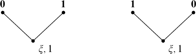


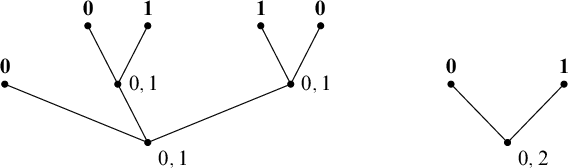

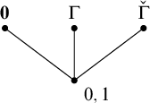

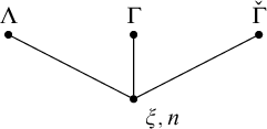

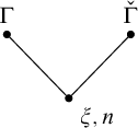


 Open access