

1. Introduction
Outburst floods from water trapped within intraglacial cavities can lead to extreme discharge events (Reference MathewsMathews, 1964; Reference HaeberliHaeberli, 1983). In densely populated mountainous areas, such abrupt floods can have catastrophic consequences on life and property (Reference Haeberli, Alean, Müller and FunkHaeberli and others, 1989). Most observed outburst floods come from intraglacial cavities in Icelandic ice caps and are also referred to as jökulhlaups (Reference Gudmundsson, Sigmundsson and BjörnssonGudmundsson and others, 1997; Reference BjörnssonBjörnsson, 1998, Reference Björnsson2003). These meltwater reservoirs result from a combination of a hydraulic pressure gradient, local topography and sometimes geothermal or hydrothermal heat (Reference BjörnssonBjörnsson, 1974; Reference NyeNye, 1976). However, the initial excavation of an outlet and intraglacial drainage processes remain unclear (Reference Fountain and WalderFountain and Walder, 1998; Reference Boon and SharpBoon and Sharp, 2003; Reference RobertsRoberts, 2005). In the Alps, outburst floods from intraglacial cavities are not rare but generally lead to only small discharges causing little or no damage (http://glaciorisk.grenoble.cemagref.fr).
The outburst flood from Glacier de Tête Rousse (Mont Blanc area), France, in 1892 was, however, one of the deadliest disasters ever caused by glaciers. Since that catastrophe, many surveys and costly investigations have been carried out to prevent similar disasters from occurring. However, the cause of the outlet excavation and outburst flood has until now remained unknown.
This study focuses on the origin of the reservoir that stored the meltwater within Glacier de Tête Rousse. It is not the intention to explain the hydromechanical opening of drainage pathways and the collapse of the tongue which led to the catastrophic outburst flood. The overall mechanism that releases such floods remains unclear.
In this paper, we successively review the historical data, analyse this event from new field data and propose an explanation on the origin of the meltwater reservoir. Note that our explanation disagrees with the conclusions of past studies. Our study should help provide a better assessment of the risks related to this glacier.
2. Historical Observations and Investigations
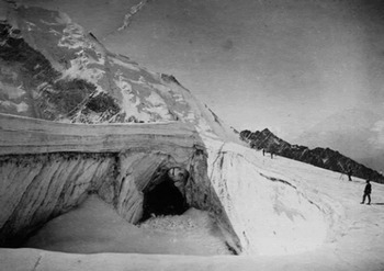
During the night of 11 July 1892 the village of SaintGervais–Le Fayet, 12 km from the town of Chamonix in the French Alps, was devastated by a water flood which caused 175 fatalities and widespread damage to infrastructure. The flood swept away everything in its path and carried with it water, boulders, soil and mud. The flood produced about 800 000 m3 of sediment. The origin of this disaster was Glacier de Tête Rousse (Fig. 1). The glacier is located in the Mont Blanc range of the French Alps (45°55′ N, 6°57′ E). The normal route to access Mont Blanc crosses this glacier. Its surface area was 0.08 km2 in 2007. The glacier extends about 0.6 km westward from an elevation of about 3300 m at the upper bergschrund to 3100 m at the terminus. It is avalanche-fed in the upper part of the accumulation zone. Detailed descriptions were compiled and surveys of the glacier were carried out after the catastrophe during the summer of 1892 (Reference Vallot, Delebecque and DuparcVallot and others, 1892). A part of the snout had been torn out of the glacier. It resulted in a large cavity 40 m in diameter and 20 m high at the glacier terminus (Fig. 2). Reference Vallot, Delebecque and DuparcVallot and others (1892) mentioned that bedrock formed a sill at the foot of this cavity, referred to as the ‘lower cavity’. They estimated that the volume of the lower cavity was 20 000 m3. From this lower cavity, an 85 m long intraglacial conduit with a mean slope of 36% led to another cavity, referred to as the ‘upper cavity’. The conduit was 3 m high. The upper cavity was elliptical, with a major axis of 50 m and a minor axis of 27 m (Fig. 3). The major axis was oriented across the glacier. The cavity was open on top and 35–40 m deep. Several pictures taken after the disaster showed that the area in the vicinity of the upper cavity was flat. The detailed map of 1901 drawn at a scale of 1 :1000 confirms the presence of a depression in the glacier surface at this location. The volume of the upper cavity was estimated at 80 000 m3. As can be seen in pictures taken after the disaster (Fig. 3), horizontal snow/ice layers with a thickness of 5–10 m were observed on the walls of the upper cavity, close to the surface. Below, the ice layers were strongly tilted (Fig. 3). According to field observations after the catastrophe, Reference Vallot, Delebecque and DuparcVallot and others (1892) reported typical sub-aquatic melting features on the ice wall and concluded that the upper cavity was filled with water up to the bottom of the horizontal layers before the outburst flood. The bottom of the upper cavity was cluttered with ice blocks, and bedrock was not visible. According to Reference Vallot, Delebecque and DuparcVallot and others (1892), these ice blocks resulted from the englacial rupture of a water-filled vault. The total volume of ice and water drained out of the glacier was estimated at 200 000 m3 (Reference Mougin, Bernard and VallotMougin and Bernard, 1905). Half of this volume was water and the other half broken ice. In August 1893, the lower cavity was only 1 m high. In August 1894, the cavity was plugged and a lake appeared in the upper cavity. In 1895, the lake was not visible as the cavity was partly filled by snow. In 1897 the upper cavity was entirely covered and in 1898 it was not visible from the surface. In 1898, the authorities in charge of public safety (Administration des Eaux et Forêts) decided to drill a horizontal tunnel through the rock and ice in order to prevent water accumulation inside the glacier (Reference KussKuss, 1901). The tunnel was completed in 1899. It passed through 64 m of rock and 50 m of ice. The engineers reached the location of the former upper cavity which was identified by the change in structure from ice to firn. No water was found at this location. However, the engineers noticed that large crevasses had formed at the surface of the glacier downstream of the former upper cavity. In 1901, a 50 m long crevasse filled with water was observed 40 m from the former upper cavity. From probes, the depth of the crevasse was estimated at 40 m. To prevent any risk of an outburst flood, the decision was made to drain the water from this crevasse. A new tunnel was therefore drilled through the rock and ice. This work was supervised by Administration des Eaux et Forêts. The tunnel diggers reached the crevasse on 28 July 1904. The crevasse was drained within 4 hours. The maximum discharge was estimated at 2 m3 s−1 and the volume of released water at 22 000 m3. This tunnel has been maintained until now by Service de Restauration des Terrains en Montagne (RTM). It is supposed to prevent water accumulation close to the bedrock of the glacier. However, over the last 105 years, no water has been drained through this tunnel. The necessity of maintaining the tunnel is therefore in doubt. In this respect, the important question concerns the origin of the meltwater reservoir of the upper cavity before July 1892. Until now, it has remained enigmatic.
View of Glacier de Tête Rousse. Photograph by B. Jourdain.

The lower cavity at the terminus of the glacier. A part of the snout has been torn from the glacier. Photograph by H. Pelloux, September 1892.

The upper cavity at the centre of the glacier. Photograph by M. Kuss, 13 August 1893.
3. New Data
Additional field measurements were performed in 2007 (Reference Vincent, Garambois, Le Meur, Thibert and LefebvreVincent and others, 2008) to allow a new analysis of the risk of another outburst flood.
3.1. Thickness variations and cumulative mass balance between 1901 and 2007
Geodetic measurements were carried out in 1901 by engineers of Les Eaux et Forêts to produce an accurate map from which a digital elevation model (DEM) of the surface of the glacier was obtained (Reference Mougin and BernardMougin and Bernard, 1922). The geodetic measurements were likely accurate to within less than ±20 cm. Two former geodetic marks were found close to the glacier and were used for the new topographic measurements in 2007. The measurements were performed by Laboratoire de Glaciologie et Géophysique de l’Environnement (LGGE), Grenoble, with a differential GPS method using the L1 and L2 frequencies and a baseline of <1 km. The coordinates are known with an accuracy better than ±0.05 m in the horizontal and vertical directions. From these data, it was therefore easy to compare the DEMs. The thickness variations between 1901 and 2007 are generally 15–20 m. The four measured cross sections are shown in Figure 4. Topographic measurements had already been made in 1950 on the same cross sections. The DEMs were constructed using Surfer software with a grid of 10 m × 10 m and a minimum curvature algorithm. The algorithm chosen for DEM construction has a weak impact on the calculated volume for the whole glacier (Reference Thibert, Blanc, Vincent and EckertThibert and others, 2008). The subtraction of the DEMs yields elevation variations that must be converted to water equivalent using the ice density, i.e. 900 kg m−3. From these data, the long-term cumulative mass balance was obtained for the period 1901–2007.
Map of surface and bedrock topography in 2007. The locations of the upper cavity and lower cavity (green dashed curve), ablation stakes (large points) and transversal cross sections (black) are shown. The longitudinal cross section of Figure 7b (blue) is also shown.

3.2. Bedrock topography
Ground-penetrating radar (GPR) has been used successfully on temperate glaciers to map bedrock geometry (Reference Arcone, Lawson and DelaneyArcone and others, 1995) or to study the distribution of water in polythermal glaciers (e.g. Reference Murray, Gooch and StuartMurray and others, 1997; Reference Moran, Greenfield, Arcone and DelaneyMoran and others, 2000; Reference Irvine-Fynn, Moorman, Williams and WalterIrvine-Fynn and others, 2006; Reference Barrett, Murray, Clark and MatsuokaBarrett and others, 2008).
The bedrock topography of Glacier de Tête Rousse was determined from GPR data using a 250 MHz shielded antenna (antenna spacing of 36 cm) connected to a RAMAC/GPR system (MALA Geosciences). The antenna proved to be satisfactory, providing high vertical resolution images of the glacier (wavelength of 70 cm for a wave propagation velocity of 175 m μs−1 within the glacier), with waves penetrating deep enough to reach the glacier–bedrock interface. GPR measurements were carried out on six cross sections and two longitudinal sections, with a spacing of 50 cm between measurements along a given section. In addition, common-midpoint (CMP) measurements were performed close to the centre of the glacier (the thickest part) to obtain the electromagnetic velocity as a function of depth. CMP analysis suggests a complex velocity profile at this location. Indeed, both semblance analyses and hyperbolic picking show a small negative gradient within the first 45 m (from 175 to 173 m μs−1) followed by large velocity variations (increasing then decreasing) at greater depths.
For each profile, a classical data-processing chain was applied (Reference Davis and AnnanDavis and Annan, 1989) consisting of (1) direct current suppressing, (2) (10–400 MHz) bandpass filtering, (3) static corrections (elevation), (4) velocity analysis, (5) frequency–wavenumber (f-k) migration, (6) time-to-depth conversion and (7) amplitude equalization. Examples of travel time diagrams and depth-migrated data are given in Figure 5a and b, respectively. The north–south cross section shown in Figure 5 is very near (within 30 m of) cross section C shown in Figures 4 and 6. On both diagrams, the direct wave corresponds to the glacier surface after applying static corrections. Figure 5a clearly shows the glacier–bedrock interface, which appears highly disturbed, with a large amount of spread energy (scattering, reflectors) in the vicinity of this interface. A great deal of scattering also appears within the glacier, characterized by a large spatial variability. Scatter density is very high at the base of the glacier, particularly in its deepest part and in a localized western part, where debris accumulation close to the bedrock–glacier dipping interface could be present. In other regions, scattering is more sparsely present together with east–west dipping continuous events in the eastern part. An f-k time migration was performed using the Stolt algorithm (1978), which is a fast-running and easyto-implement migration method well adapted to dipping corrections when constant velocity is assumed (here v = 175 m μs−1). The depth-migrated profile is reported in Figure 5b, where scattering hyperbola effects have been strongly attenuated by focusing scattering energy and correctly relocating dipping interfaces.
North–south GPR data using a 250 MHz antenna. (a) Data after elevation corrections and amplitude equalization. (b) Data derived from (a) after f-k migration and time-to-depth conversion (with a velocity of 175 m μs−1). The cross sections are seen from downstream.

Cross sections a, b, c and d. The scales are the same for all the graphs. The cross sections are seen from downstream.

The amount of scattering clutter was definitely increased by the high-frequency antenna used in this study (Reference Watts and EnglandWatts and England, 1976), which increases the detection power for small objects such as debris inclusions and englacial water. Despite the absence of clear out-of-plane reflections, interface geometry was difficult to determine on all profiles due to energy spreading. It could, however, be defined to within 1–3 m depending on the studied profiles, making it possible to obtain a pseudo-three-dimensional image of the bedrock topography as shown in Figures 4 and 6. Scattering observed all along the interface may be due to the small-scale roughness of the interface geometry, the presence of till rocks and/or the fractures affecting the bedrock material.
3.3. Temperature measurements
The ice temperature was monitored by five thermistors with an accuracy of 0.1°C, installed in five 7.90–11.90 m deep boreholes used for ablation stakes on 23 September 2007 (Table 1; Fig. 4). The firn layers were 1.60 and 0.90 m thick at the upper boreholes. The other sites were free of firn. Two other thermistors were set up in ice at the base of the glacier close to the bedrock, accessed through the tunnel drilled in the rock in 1904. Temperatures were obtained 2 weeks after drilling completion on 2 October 2007, on 9 September 2008 and again on 11 September 2009 in the same boreholes. These borehole temperatures were consistent (±0.1°C). Table 1 shows all the ice temperature measurements. The basal temperatures measured in the tunnel were both about −2.5°C. The 12 m deep borehole temperatures reveal a striking horizontal temperature gradient, with warmer englacial temperatures in the upper part of the glacier. This gradient is likely related to the snow accumulation pattern on the glacier and can be explained as follows. During winter, the snow layer at the glacier surface cools due to a strong net loss of energy. In spring and summer, the winter snow layer warms due to the release of latent heat through the freezing of percolating meltwater coming from surface melt. In the accumulation area, this heat flow is significant over the entire summer season. In the ablation area, when the winter snow layer has been removed, the impermeable ice surface prevents any percolation of meltwater. Consequently, the ice can only be warmed by conduction. Given that ice is a poor conductor, this heat flow is low. These processes have been identified as the origin of polythermal glaciers (Reference Petterson, Jansson, Huwald and BlatterPettersson and others, 2007). Tests based on heat-flow numerical modelling (Reference Vincent, Le Meur, Six, Possenti, Lefebvre and FunkVincent and others, 2007) have been performed to estimate how the seasonal surface temperature variations influence the temperature in ice. These numerical experiments indicate that the temperature variations are less than ±0.2°C at 12 m depth. As a result, the 12 m deep temperature corresponds to the yearly average temperature. Although the temperature measurements are sparse, they indicate that the glacier is likely cold over most of its area. This conclusion conflicts with ice temperature measurements carried out at the beginning of the 20th century. Indeed, from ice temperature measurements performed between 1901 and 1903, Reference MouginMougin (1904) and Mougin and Bernard (1905) concluded that this glacier was temperate. These measurements were carried out at two locations, 15 and 20 m below the surface, in the ice tunnel dug in 1899. Given that these measurements were performed with calibrated instruments (±0.1 °C), there is no objective reason to doubt their accuracy. Note, however, that the temperature measurements recorded between 1901 and 1903 were made in the upper half of the glacier. These results are discussed below in section 5.
Temperature measurements in boreholes

3.4. Ice-flow measurements
The surface ice-flow velocities were measured at the end of the ablation season in 2007 and 2009 (September) from five ablation stake displacements on a longitudinal section of the glacier. Measurements were made using a differential GPS method and are known with an uncertainty of ±0.05 m a−1. The ice-flow velocities range from 0.4 to 0.6 m a−1. In addition, many ice-flow velocity measurements were carried out between 1901 and 1903 on the four cross sections shown in Figure 4 (Reference Mougin and BernardMougin and Bernard, 1922). The displacement of 10–20 painted stones was measured using topographic methods (theodolite surveys). The ice-flow velocities range from 0.2 m a−1 close to the edge of the glacier to 1.1 m a−1 at the centre. Although our data from 2007 and 2009 do not allow a detailed comparison with the data obtained between 1901 and 1903, the findings do suggest that the ice-flow velocity of this glacier is low and has not changed significantly over the last century.
3.5. Surface mass-balance measurements
Winter and summer surface mass balances were obtained from measurements performed on 2 October 2007, 7 May 2008 and 9 September 2008 from drilled cores and the five ablation stakes. The winter mass balance was +0.83 m w.e. and the summer mass balance −1.41 m w.e. In addition, accumulation and ablation measurements were carried out between 1901 and 1903 from stakes and pits. The winter mass balances were +0.42 and +0.39 m w.e. in 1901/02 and 1902/03, respectively. The summer mass balances were −0.50 and −0.64 m w.e. in 1901/02 and 1902/03, respectively (Administration des Eaux et Forêts, 1913; Reference Mougin and BernardMougin and Bernard, 1922).
4. Analysis of the Origin of the Outburst Flood
4.1. Previous analysis
According to Reference Vallot, Delebecque and DuparcVallot and others (1892) and Reference VallotVallot (1894), the englacial cavities were the result of crevasses that became filled with meltwater. Following the disaster, these authors mentioned that they observed several large crevasses which were larger below the surface than at the surface. Unfortunately, the field reports do not give any details about the location of these crevasses. Nine years after the catastrophe, in 1901, Reference Mougin and BernardMougin and Bernard (1922) confirmed the existence of such crevasses. At a position 40 m from the former upper cavity, they observed a 50 m long crevasse with a width of 1 m at the surface and 4 m at 2 m depth. Below, the walls were parallel down to 30 m depth and then widened down to 40 m depth. This crevasse was filled with water and the volume was estimated at 20 000 m3. The shape of these crevasses was believed to be the consequence of the concave bedrock topography. Reference Vallot, Delebecque and DuparcVallot and others (1892) reported a sill in the bedrock at the terminus, at the foot of the lower cavity (Fig. 7a). This sill implies a concave shape in the bedrock upstream. For this reason, Reference Vallot, Delebecque and DuparcVallot and others (1892) assumed that there was a similar sill upstream, which was believed to be the origin of the upper cavity (Fig. 7a). However, they could not check this assumption as they were not able to measure the bedrock topography. According to Reference VallotVallot (1894), the lower cavity resulted from a former cavity formed at the location of the upper cavity, which had moved downstream with the ice flow. Assuming ice-flow velocities of 2–3 m a−1, which had not yet been measured, Reference VallotVallot (1894) concluded that more than 50 years were required to reach the terminus of the glacier located 140 m from the upper cavity. Finally, he assumed that the englacial rupture of the water-filled vault in the upper cavity triggered a high water pressure leading to the opening of drainage pathways, the breaking-off of the snout and the abrupt release of water from the glacier.
Longitudinal section of the tongue. (a) Sketch from Reference Vallot, Delebecque and DuparcVallot and others (1892). The bedrock was not measured. (b) Cross section from our measurements.

Many of these assumptions are questionable. First, our radar measurements do not reveal any marked concave shape of the bedrock (Figs 4 and 7b). Consequently, the assumption made by Reference VallotVallot (1894) concerning the opening of the deeper part of the crevasse due to the concave shape of the bedrock is not supported by our measurements. Secondly, the topographic measurements performed between 1901 and 1903 reveal low surface ice-flow velocities of about 1.1 m a−1 at the centre of the glacier. Additional ice-flow measurements between 1903 and 1950 (Reference ChaumetonChaumeton, 1950) show similar results. As mentioned above, the horizontal ice-flow velocity was 0.6 m a−1 at the centre of the glacier between 2007 and 2009. All these results indicate that extending flow in the horizontal directions is small and cannot lead to the opening of large crevasses. Consequently, in the area of the upper cavity, in the flat area, the longitudinal strain rate should not have exceeded 0.01 a−1 in 1892, which is less than the value of 0.03 a−1 at which the crevasses form (Reference Meier, Kamb, Allen and SharpMeier and others, 1974). The large crevasses mentioned by Reference Vallot, Delebecque and DuparcVallot and others (1892) after the disaster were observed downstream of the upper cavity, i.e. downstream of the slope change. Furthermore, as discussed in section 5, these crevasses and their shapes could be related to changes in ice-flow dynamics after the outburst flood. The crevasse found in 1901, 40 m downstream of the upper cavity, probably results from the change in tensile stress in the vicinity of the glacier tongue after the outburst flood and was kept open by the water it contained. Thirdly, Reference Vallot, Delebecque and DuparcVallot and others (1892) supposed that the crevasse that was the origin of the upper cavity had been enlarged by wall melting by water coming from surface melting. However, the water coming from surface melting would have been cold, close to 0°C (Reference Isenko, Naruse and MavlyudovIsenko and others, 2005). Consequently, the thermal energy in the water transferred to the ice for melting would have been very low and not sufficient to have a large impact on the enlargement of a crevasse. Assuming that all the thermal energy released within the water was used to melt the ice and that the water temperature was 1°C, the volume of melted ice would be 250 m3 for 20 000 m3 of water. The energy brought by water from surface melting is therefore not sufficient to cause crevasse enlargement and the formation of a large englacial meltwater reservoir, as supposed by Reference Vallot, Delebecque and DuparcVallot and others (1892). Further calculations from solar radiation confirm this conclusion. Assuming a water-filled crevasse with a water surface area of 50 m2, it is possible to calculate the maximum amount of energy from solar radiation that can be absorbed by the water. To obtain an upper limit, we considered a maximum duration of 2 months without winter snow cover, an albedo of 0.04 for water, a maximum value of mean net shortwave radiation of 300 W m−2 (Reference Six, Wagnon, Sicart and VincentSix and others, 2009) and a mean net longwave radiation close to zero. Using the latent heat of fusion (L f = 334 000 J kg−1) and assuming this energy is used entirely for melting, the amount of melted ice would be 220 m3. Given that this represents an upper limit, the energy brought by solar radiation is not sufficient to enlarge a crevasse significantly.
4.2. New analysis
We propose here a new explanation for the origin of the meltwater reservoir. Looking closely at Figure 3, we note that the surface layers are very different from the deep ice layers. The surface layers are horizontal whereas the underlying ice layers are strongly tilted. The surface layers seem to correspond to recent accumulation and the deep ice layers to old ice coming from upstream, bent by the ice flow. In order to confirm this, the glacier mass balance was reconstructed for a period beginning before 1892 using meteorological data with a degree-day model and taking into account the change in the surface area of the glaciers (Reference VincentVincent, 2002). Several meteorological datasets were used to reconstruct the glacier mass balance. First, homogenized temperature (45° N, 6° E) (Reference Böhm, Auer, Brunetti, Maugeri, Nanni and SchönerBöhm and others, 2001) and precipitation (Reference AuerAuer and others, 2007) data were used to reconstruct the mass balance of Glacier de Tête Rousse between 1810 and 1998. Lyon temperature and Besse precipitation data were then used to reconstruct the mass balance between 1907 and 2007. Mass-balance values were calculated for each elevation interval (50 m). The two reconstructed cumulative specific net balances are shown in Figure 8. Surface area changes were taken into account using the maps mentioned above. The overall trend between 1901 and 2007 is constrained by glacier volume variations deduced from the 1901 map and geodetic measurements performed in 2007. In this way, reconstructed and observed glaciological mass balances have been combined, as proposed by Reference Thibert and VincentThibert and Vincent (2009), so that the cumulative mass balances between 1901 and 2007 match volumetric mass balances from geodetic measurements. First, the reconstruction from Lyon temperature and Besse precipitation was adjusted to the volumetric mass balance measured between 1901 and 2007. However, meteorological data for Lyon and Besse are available only since 1907. Between 1901 and 1907, we assume that the mass balance is close to zero. This assumption is supported partly by Les Eaux et Forêts field measurements which show that the glacier mass balance is close to zero between 1901 and 1903 (Reference Mougin and BernardMougin and Bernard, 1922). Our assumption could lead to an uncertainty of 2 or 3 m w.e. on the origin of the cumulative mass-balance curve in 1907. Secondly, the reconstruction from homogenized data (1810–1998) has been adjusted to geodetic measurements made in 1901 and the reconstructed cumulative mass balance of 1998 obtained previously. In addition, the net mass balance of Glacier d’Argentière, located 15 km away, was used to check the shape of the cumulative mass-balance curve over the last three decades. In this way, the specific cumulative net balance of Glacier d’Argentiere is reported in Figure 8, removing 0.12 m w.e.a−1, to adjust the cumulative mass balance between 1977 and 2007. These data show that (1) the reconstructed values agree roughly with volume variations obtained from geodetic measurements in 1950; and (2) both reconstructions show an overall agreement. Consequently, these reconstructions can be used to assess the surface mass balance of this glacier.
Cumulative mean specific net balance (m w.e.) of Glacier de Tête Rousse from maps (triangles), from a reconstruction using Besse precipitation and Lyon temperature data (blue curve), from a reconstruction using homogenized precipitation and temperature data (red curve) and from glaciological measurements of Glacier d’Argentière (green curve).

The reconstructed cumulative mass balance of the glacier shows a positive trend between 1878 and 1892. This positive mass balance is confirmed by the general extension of glaciers (Reference GroveGrove, 1988; Reference Vincent, Le Meur, Six and FunkVincent and others, 2005) as deduced from length observations at the end of the 19th century. The length fluctuations of Glacier des Bossons (Mont Blanc area), 3.5 km from Glacier de Tête Rousse, reveal a clear advance of 366 m between 1878 and 1892 (Reference Vincent, Le Meur, Six and FunkVincent and others, 2005). Although these length variations cannot be interpreted directly in terms of climate change, it has been shown (Reference MartinMartin, 1977; Reference Reynaud, Berger and NicolisReynaud, 1984) that this glacier has a very short response time and that these snout fluctuations are closely related to cumulative mass-balance variations. Consequently, the advance of this glacier must be caused by a period of positive mass balance. From these observations and from the reconstruction, we can conclude that the mass balances of Glacier de Tête Rousse were very likely positive between 1878 and 1892.
In addition, the surface mass balance has been reconstructed between 1850 and 1910 using the same method at the elevation of the upper cavity. Consequently, for this calculation, the surface change of the glacier is not taken into account. As expected from previous results, the cumulative mass balance shows a positive trend between 1878 and 1892, although mass balances were negative in 1879/80, 1880/81, 1883/84 and 1884/85. Conversely, the mass balance was strongly negative over the previous decade, i.e. 1867–78. This reconstruction confirms our assumption that the surface horizontal layers seen in Figure 3 correspond to positive mass balance between 1877 and 1892. In addition, according to field observations by Reference Vallot, Delebecque and DuparcVallot and others (1892), the appearance of ice in the upper cavity reveals that the deep ice layers were in contact with water and that the cavity was very likely filled with water up to the bottom of the horizontal layers before the outburst flood.
These results and observations lead to the conclusion that the origin of the water reservoir was very likely a supraglacial lake formed before 1878, during the period of negative mass balance. Over this period, the surface of the lake was frozen in winter and covered by snow. During summer, the lake was free of ice and warmed under the influence of solar radiation and air temperature. In addition, the warming was strengthened by thermal convection. The lake was therefore enlarged by the ice melted by energy from solar radiation. Recent studies on supraglacial Lac de Rochemelon, France, have shown that the melting of ice can reach 15 cm d−1 during summer over the edge of the lake (Reference Vincent, Auclair and Le MeurVincent and others, 2010). During the winter of 1878/79, as in previous winters, the lake was covered by an ice layer. It was covered by snow accumulation but this snow layer did not melt during the summer of 1879. Given that the mean surface mass balance was positive between 1878 and 1892, the lake was hidden from the surface until the outburst flood of 1892.
The surface topography features support our assumption relative to a supraglacial lake formed between 1867 and 1878. Indeed, the pictures taken after the disaster show that the area in the vicinity of the upper cavity was flat. Moreover, the map drawn in 1901 (Reference Mougin and BernardMougin and Bernard, 1922) shows a flat area at the glacier surface about 20–30 m upstream of the upper cavity location in 1892. Given that the ice-flow velocity was ∼1 m a−1 in this area, the upper cavity should have been located in this flat area 20–30 years before 1892, indicating that the origin of the meltwater reservoir was a supraglacial lake. The elliptical shape of the upper cavity could come from the shape of the flat area in which the meltwater spread according to the depression outlined by the contour lines. Many of the ponds formed on alpine glaciers are larger in the direction perpendicular to the ice flow. Owing to solar radiation, the lake was enlarged and deepened. Under the influence of solar radiation during summer, the warming is enhanced by the thermal convection. Given that the density of fresh water is maximum when temperature reaches +4°C, the warmer surface water sinks to the lake bottom, flows toward the ice walls and cools (Reference Haeberli, Kääb, Vonder Mühll and TeysseireHaeberli and others, 2001). The density therefore decreases and the water rises again to the lake surface. Observations from supraglacial lakes in other studies show that the ice walls of several of these lakes were vertical (Reference RöhlRöhl, 2008; Reference Vincent, Auclair and Le MeurVincent and others, 2010; personal communication from L. Mercalli, 2008). For instance, the cavity of Lac de Rochemelon exhibited up to 20 m vertical ice walls before the lake was drained artificially (Reference Vincent, Auclair and Le MeurVincent and others, 2010). Other studies show that supraglacial ponds on glaciers can easily reach depths up to 30–40 m (Reference Mortara and MercalliMortara and Mercalli, 2002; Reference RöhlRöhl, 2008). Finally, the depth of the lake in the upper cavity of Glacier de Tête Rousse reached 25–30 m before it was covered by snow layers due to positive mass balance after 1878.
5. Discussion
Careful analysis has been performed to study whether the reservoir of the upper cavity could come from an enlarging crevasse. According to this assumption, growth of a water-filled crevasse could result from two mechanisms: (1) the melting of the ice walls by the thermal energy in the water; and/or (2) the hydrologically driven propagation of fractures. We do not believe that these mechanisms were efficient in the case of Glacier de Tête Rousse. First, as explained in section 4.1, the thermal energy in the water coming from surface melting is very low and not sufficient to significantly enlarge a crevasse. The second mechanism is related to the water pressure. The water pressure is sufficient to deepen a crevasse (Reference Van der VeenVan der Veen, 2007) but not to widen it. According to literature, water-filled crevasses can penetrate the full ice thickness of glaciers (Reference WeertmanWeertman, 1973; Reference Van der VeenVan der Veen, 1998). Reference Van der VeenVan der Veen (2007) showed that a crevasse subjected to inflow of water will propagate downwards, with the propagation speed controlled primarily by the rate of injection, independent of the value of the far-field tensile stress. For this reason, the mechanism is not efficient to widen a crevasse. Indeed, if the water pressure compensates for the lithostatic stress in the ice, the crevasse propagates downward with a velocity similar to the rate of injection (Reference Van der VeenVan der Veen, 2007). On the other hand, if the water pressure does not compensate for the lithostatic stress in the ice, the crevasse does not penetrate deeper and will be sealed. In this case, the water level will decrease due to the widening of the crevasse until the water pressure has dropped sufficiently to make further widening impossible. Extensive crevasse widening from water pressure should therefore not be very efficient. Moreover, field observations do not support the assumption of an enlarging crevasse. Indeed, if the upper cavity were a crevasse and if the water pressure were the cause of the enlargement of the crevasse, the distance between the ice walls would increase with depth. However, no overhanging ice walls were observed in the upper cavity. On the contrary, Reference Vallot, Delebecque and DuparcVallot and others (1892) indicated that the ice walls were vertical.
The explanations concerning the origin of the upper cavity do not explain how the water penetrated the glacier via an englacial conduit and formed another cavity close to the terminus. This topic is discussed here although no firm conclusions may be drawn. The overall mechanism that releases a flood from a supraglacial lake appears to be a combination of a hydraulic pressure gradient, local topography, ice fracturing and ice temperature (Reference BjörnssonBjörnsson, 1974; Reference NyeNye, 1976; Reference Sturm and BensonSturm and Benson, 1985; Reference Boon and SharpBoon and Sharp, 2003). The mechanisms driving the penetration are not well understood. The supraglacial lake drains in response to the hydromechanical opening of drainage pathways (Reference RobertsRoberts, 2005). Observations from a sub-temperate glacier on Ellesmere Island, Canada, suggest that the penetration mechanism may involve water-pressure-induced ice fracturing (Reference Boon and SharpBoon and Sharp, 2003). In the case of Glacier de Tête Rousse in 1892, the water level in the upper cavity was close to 3167 ± 3 m. The elevation of the englacial conduit entrance was close to 3132 ± 3 m, which means that the hydrostatic water pressure there was 0.35 ± 0.06 MPa. Taking into account the uncertainty concerning the snow layer thickness at the glacier surface, the ice pressure was 0.36 ± 0.02 MPa at this point. This suggests that the hydrostatic water pressure was close to the ice pressure, not sufficient alone to excavate a tunnel in the glacier (Reference Van der VeenVan der Veen, 1998) but sufficient to keep a conduit open. The opening of the englacial conduit remains unclear and is likely related to fractures allowing floodwater to race toward the fracture tip with each successive split (Reference Fountain, Jacobel, Schlichting and JanssonFountain and others, 2005; Reference RobertsRoberts, 2005). It also suggests that ice was temperate in the vicinity of the conduit, given that it seems unlikely that water entering small cracks can carry or generate enough heat to develop a conduit within cold ice (Reference PatersonPaterson, 1994, p.125).
The water from surface melting increased the water level and the water pressure, opening the englacial conduit. As the excavation of the tunnel advanced down the glacier, the height of the water above the front of the tunnel increased, thereby increasing the hydrostatic pressure and possibly explaining the funnel shape of the conduit.
Finally, from field observations, it appears that the englacial conduit reached the bedrock and led to the formation of the lower cavity. The lower cavity must have been watertight, otherwise the water would have been released to the glacier surface through a crevasse or from the terminus through a subglacial conduit. Given that the bottom of the lower cavity was bedrock, the tongue must have been frozen to the bedrock and consequently cold. The cause of the breaking of the terminus remains unclear. Two possible origins can be considered. First, the glacier terminus could have been broken by the thinning of the ice above the lower cavity. It would have collapsed due to the resulting water pressure. Another possibility could be related to the change in thermal conditions. Owing to ice warming, the tongue may have become temperate and the water released through a subglacial conduit. In this case, the release mechanism involves lifting the ice off a critical seal (Reference Sturm and BensonSturm and Benson, 1985; Reference RobertsRoberts, 2005; Reference Sugiyama, Bauder, Huss, Riesen and FunkSugiyama and others, 2008), resulting in collapse of the terminus. In any case, we believe that the glacier terminus was cold before 1892, forming a watertight cavity in contact with the bedrock.
According to ice temperature measurements performed in 1901, the glacier was temperate. Our measurements performed in 2007 revealed that the glacier is cold. This suggests that the thermal conditions of this glacier can change depending on the surface energy fluxes, accumulation rate and ice thickness. The mass-balance reconstruction (Fig. 9) shows that mass balance was on average positive between 1878 and 1892. Given that ice temperature depends strongly on the thickness of the snow layer on the glacier (Reference PatersonPaterson, 1994, p.209), the positive mass balance would have led progressively to temperate conditions between 1878 and 1892. In addition, the collapse of the terminus and the outburst flood likely changed the ice-flow dynamics. The outburst flood very likely reduced basal shear traction close to the terminus, resulting in local acceleration of the ice flow (Reference Iken, Röthlisberger, Flotron and HaeberliIken and others, 1983; Reference Kamb and EngelhardtKamb and Engelhadt, 1987; Reference Kavanaugh and ClarkeKavanaugh and Clarke, 2001). This would increase the longitudinal velocity gradient and the tensile stress in the vicinity of the glacier tongue, resulting in crevasse widening. This could explain the large crevasses found downstream of the upper cavity after the disaster.
Cumulative surface net balance (m w.e.) at the elevation of the former upper cavity (3165 m a.s.l.) between 1850 and 1910 from a reconstruction using homogenized precipitation and temperature data.

6. Conclusions
We have taken a new look at the origin of the meltwater reservoir in the upper cavity observed in Glacier de Tête Rousse in 1892. Reference Vallot, Delebecque and DuparcVallot and others (1892) assumed that this reservoir resulted from a crevasse filled by water coming from surface ice melting. However, the assumption of Reference Vallot, Delebecque and DuparcVallot and others (1892) concerning the opening of the bottom of the crevasse by the concave shape of the bedrock surface is not supported by our measurements. Our new analysis shows that the reservoir of the upper cavity could not come from an enlarging crevasse. First, our measurements, as well as the measurements performed in 1901, indicate that horizontal ice-flow velocities are small and cannot lead to the opening of large crevasses. Second, the ice deformation in a water-filled crevasse resulting from water pressure is not sufficient to widen a large crevasse far below the surface. Moreover, the field observations of vertical walls conflicts with this possible mechanism. Third, the thermal energy in the water transferred to the ice for melting is not sufficient to have a large impact on the enlargement of a crevasse.
Our study shows that the origin of the meltwater reservoir was more likely a supraglacial lake. First, the pictures taken and the map drawn after the disaster indicate that the area upstream of the upper cavity was flat. Second, careful inspection of the upper cavity pictures taken after the disaster shows that the surface layers correspond to recent accumulation. Mass-balance reconstructions confirm that the surface layers correspond to a positive mass balance between 1878 and 1892, whereas the surface mass balance was strongly negative over the previous decade. Third, according to field observations after the outburst flood, the upper cavity was filled with water up to the bottom of the surface layers. Fourth, the solar radiation captured all over the lake area is necessary to widen significantly a water-filled cavity. We cannot exclude the possibility that a water-filled crevasse was the origin of the pond and that this crevasse was fed by a supraglacial lake. However, the only efficient way to provide enough heat to enlarge significantly the water-filled cavity lies in the solar energy collected over a large area.
All these results and observations suggest that the origin of the upper cavity was very likely a supraglacial lake that was covered by snow accumulation between 1878 and 1892. Before 1878, the glacier was not a popular location and the lake could have gone unnoticed. If this was the case, it would mean that this hazard could have been detected easily from the surface before the lake was hidden.
This conclusion could be very important for the authorities in charge of managing the potential risk of another outburst flood from Glacier de Tête Rousse. Unfortunately, we have not found any pictures or reports of this glacier over the period 1867–78. In the future, a thorough historical search for the existence of a potential supraglacial lake before 1878 is required. No firm conclusion can be drawn without this proof.
The mechanisms by which the water penetrated into the glacier to form an englacial conduit and the lower cavity, finally leading to the breaking of the terminus, remain unclear. The collapse could be related to a change in the thermal conditions of the glacier. Our measurements reveal that the glacier was cold in 2007, although it was temperate at the beginning of the 20th century. These data show that the thermal conditions can change with time. In the future, we propose to study the temperature distribution of this glacier in the past from a heat-transfer model using meteorological data and mass-balance reconstruction. This could provide information on the temperature of the ice in the vicinity of the terminus in 1892.
Finally, we propose an overall mechanism of this outburst flood, although it remains speculative. This outburst flood hazard could be related to change in mass balance. First, following a negative mass-balance period, the glacier may have become cold. Moreover, these negative mass balances would have led to the formation of a supraglacial lake in a flat area of the glacier. At the end of this period, the supraglacial lake would have been covered by snow accumulation during a new positive mass-balance period. Owing to this snow accumulation increase, the ice temperature would have increased. Depending on water pressure and ice temperature, a funnel-shaped englacial conduit could have formed, leading to the formation of the lower cavity. The lower cavity would have been watertight due to the cold ice of the tongue. Through progressive ice warming due to a positive mass balance, the tongue may have become temperate and the water release would result in collapse of the terminus and the outburst flood.
Acknowledgements
We thank all who have taken part in collecting the field measurements on Glacier de Tête Rousse. This study has been funded by Service de Restauration des Terrains en Montagne (RTM) of Haute Savoie (France), by the town of Saint-Gervais (France) and by the GlaRIskAlp Alcotra programme. We thank R. Böhm and his team for the homogenized meteorological data. We thank N. Karr and V. Tairraz for advice and for taking part in the collection of the field measurements. We are very grateful to M.T. Gudmundsson, M. Funk and an anonymous reviewer whose comments greatly improved the clarity of the manuscript.


