
 {log}
{log}


1 Introduction
The work presented in this paper is aligned with the following quotations (Garavel et al. Reference Garavel, ter Beek and van de Pol2020).
The introduction of programming languages supported by proof systems. I do expect it to become more common with programming language implementations being born with program verifiers of various kinds. […] It is a pleasure to see modern programming languages to an increasing degree look and feel like well known formal specification languages.
Klaus Havelund
Another challenge is to better integrate specification and proof with programming, preferably at the level of programming languages and tools.
Xavier Leroy
That is, this paper presents $\{log\}$
(read ‘setlog’) (Rossi and Cristiá Reference Rossi and Cristiá2000; Dovier et al. Reference Dovier, Piazza, Pontelli and Rossi2000), a programming language that has the look-and-feel of a formal specification language which in turn is supported by a proof system. The core of
$\{log\}$
(read ‘setlog’) (Rossi and Cristiá Reference Rossi and Cristiá2000; Dovier et al. Reference Dovier, Piazza, Pontelli and Rossi2000), a programming language that has the look-and-feel of a formal specification language which in turn is supported by a proof system. The core of $\{log\}$
is a Constraint Logic Programming (CLP) language and interpreter written in SWI-Prolog implementing a constraint satisfiability solver for set theory. The satisfiability solver is a rewriting system implementing decision procedures for several fragments of set theory (e.g., integer intervals (Cristiá and Rossi Reference Cristiá and Rossi2024c) and restricted quantifiers (RQ) (Cristiá and Rossi Reference Cristiá and Rossi2024d)). In this way,
$\{log\}$
is a Constraint Logic Programming (CLP) language and interpreter written in SWI-Prolog implementing a constraint satisfiability solver for set theory. The satisfiability solver is a rewriting system implementing decision procedures for several fragments of set theory (e.g., integer intervals (Cristiá and Rossi Reference Cristiá and Rossi2024c) and restricted quantifiers (RQ) (Cristiá and Rossi Reference Cristiá and Rossi2024d)). In this way, $\{log\}$
implements declarative programming in the form of set programming (Schwartz et al. Reference Schwartz, Dewar, Dubinsky and Schonberg1986; Cantone et al. Reference Cantone, Omodeo and Policriti2001). As such
$\{log\}$
implements declarative programming in the form of set programming (Schwartz et al. Reference Schwartz, Dewar, Dubinsky and Schonberg1986; Cantone et al. Reference Cantone, Omodeo and Policriti2001). As such $\{log\}$
has been applied to several case studies showing that the satisfiability solver works in practice (Cristiá and Rossi Reference Cristiá and Rossi2021a,Reference Cristiá and Rossic, Reference Cristiá and Rossi2024a; Cristiá et al. Reference Cristiá and Rossi2023; Capozucca et al. Reference Capozucca, Cristiá, Horne and Katz2024).
$\{log\}$
has been applied to several case studies showing that the satisfiability solver works in practice (Cristiá and Rossi Reference Cristiá and Rossi2021a,Reference Cristiá and Rossic, Reference Cristiá and Rossi2024a; Cristiá et al. Reference Cristiá and Rossi2023; Capozucca et al. Reference Capozucca, Cristiá, Horne and Katz2024).
However, writing good $\{log\}$
code, adding the corresponding verification conditions (VCs) and passing them to the satisfiability solver as to ensure the code verifies some properties, can be cumbersome. In this context, good
$\{log\}$
code, adding the corresponding verification conditions (VCs) and passing them to the satisfiability solver as to ensure the code verifies some properties, can be cumbersome. In this context, good $\{log\}$
code means code for which it is easy to write down VCs that can be automatically discharged by
$\{log\}$
code means code for which it is easy to write down VCs that can be automatically discharged by $\{log\}$
. As a programming language,
$\{log\}$
. As a programming language, $\{log\}$
includes many programming facilities leading to code that is not always easy to verify because, many times, lies outside the fragments of set theory for which
$\{log\}$
includes many programming facilities leading to code that is not always easy to verify because, many times, lies outside the fragments of set theory for which $\{log\}$
implements decision procedures. Hence, if a VC is given by a
$\{log\}$
implements decision procedures. Hence, if a VC is given by a $\{log\}$
formula for which no decision procedure can be applied,
$\{log\}$
formula for which no decision procedure can be applied, $\{log\}$
will not be able to automatically discharge it. This, in turn, implies less reliable code that needs more human effort to be verified.
$\{log\}$
will not be able to automatically discharge it. This, in turn, implies less reliable code that needs more human effort to be verified.
For these reasons, over the years, $\{log\}$
has been extended with some components (also implemented in SWI-Prolog) that constrain programmers to write code that is easier to verify. This programming style within
$\{log\}$
has been extended with some components (also implemented in SWI-Prolog) that constrain programmers to write code that is easier to verify. This programming style within $\{log\}$
defines a language for the description of state machines in terms of first-order logic (FOL), set theory and integer arithmetic – much as in formal notations such as B (Abrial Reference Abrial1996) and Z (Woodcock and Davies Reference Woodcock and Davies1996). In this way: (i) the state machine language allows for the automatic generation of VCs; (ii) these VC are automatically fed into the satisfiability solver which informs the user if they could be discharged or not (in which case, a counterexample is generated); (iii) state machines can still be executed as regular
$\{log\}$
defines a language for the description of state machines in terms of first-order logic (FOL), set theory and integer arithmetic – much as in formal notations such as B (Abrial Reference Abrial1996) and Z (Woodcock and Davies Reference Woodcock and Davies1996). In this way: (i) the state machine language allows for the automatic generation of VCs; (ii) these VC are automatically fed into the satisfiability solver which informs the user if they could be discharged or not (in which case, a counterexample is generated); (iii) state machines can still be executed as regular $\{log\}$
code thus allowing users to use them as working functional prototypes before attempting any serious proof campaign; and (iv) users can generate test cases to test a future, more efficient implementation written in some other programming language. This paper makes a comprehensive presentation of these extensions aiming at showing how theoretical contributions in the fields of CLP and set programming can be turned into a feasible tool aimed at formal verification.
$\{log\}$
code thus allowing users to use them as working functional prototypes before attempting any serious proof campaign; and (iv) users can generate test cases to test a future, more efficient implementation written in some other programming language. This paper makes a comprehensive presentation of these extensions aiming at showing how theoretical contributions in the fields of CLP and set programming can be turned into a feasible tool aimed at formal verification.
As the above quotations suggest, there are other systems where programming and proof coexist. Four conspicuous, widely known, successful representatives of this kind are AGDA (Norell Reference Norell2008; Logic and Types group 2004), DAFNY (Leino Reference Leino2010a, Reference Leinob), F* (read ‘f-star’) (Swamy et al. Reference Swamy, Hritcu, Keller, Rastogi, Delignat-Lavaud, Forest, Bhargavan, Fournet, Strub, Kohlweiss, Zinzindohoue and Zanella-Béguelin2016; Microsoft Research and INRIA 2015) and WHY3 (Bobot et al. Reference Bobot, Filliâtre, Marché and Paskevich2011; Toccata group 2012). All of them have been applied to a range of problems, some times of industrial size and complexity.
AGDA is a typed functional programming language and proof assistant based on intuitionistic type theory. The functional language provides usual functional features such as inductive types, pattern matching, and so on. Proofs are interactive and written in a functional programming style that, unlike Coq (now renamed as Rocq) (Bertot and Castéran Reference Bertot and Castéran2004), does not provide proof tactics. Programmers can, nonetheless, implement AGDA functions that return a proof of some property.Footnote 1 These functions embody sort of proof tactics. Later, these functions are run during type checking: if one of them fails, then type checking fails. This means that the program does not verify a certain property. As a form of proof automation AGDA provides proof search by enumerating possible proof terms that may fit in the specification.
DAFNY combines ideas from the functional and imperative paradigms, including some support for object-oriented programming. Programs are annotated with specifications through preconditions, postconditions, loop invariants, etc. The specification language has the look-and-feel of a programming language including mathematical integers, bit-vectors, sequences, sets, induction, and so on. Proof obligations are automatically discharged, given sufficient specification, by the Z3 SMT solver (de Moura and Bjørner Reference de Moura and Bjørner2008; Microsoft Research 2008). Sufficient specification means, in general, to write sufficient proof steps (e.g., the inductive step in an inductive proof) the remainder of which are discharged automatically.
F* supports purely functional programming as well as effectful programming (McBride and Paterson Reference McBride and Paterson2008). Its powerful (dependent) type system allows to describe precise program specifications including security and functional properties. The typechecker will check whether or not the program verifies its specification by discharging proofs interactively written by the programmer (using tactics, metaprogramming and symbolic computation) or by calling the Z3 SMT solver.
Why3 is a platform for deductive program verification. It provides WhyML, a specification and programming language. Why3 uses many external theorem provers (e.g., Alt-Ergo (OCamlPro 2006; Conchon et al. Reference Conchon, Iguernelala and Mebsout2013), CVC4-5 (Barrett et al. Reference Barrett, Conway, Deters, Hadarean, Jovanovic, King, Reynolds and Tinelli2011; Barbosa et al. Reference Barbosa, Barrett, Brain, Kremer, Lachnitt, Mann, Mohamed, Mohamed, Niemetz, Nötzli, Ozdemir, Preiner, Reynolds, Sheng, Tinelli and Zohar2022) and E-prover (Schulz Reference Schulz1999; Schulz et al. Reference Schulz, Cruanes and Vukmirovic2019)) to discharge proof obligations. The system includes a library of mathematical theories (e.g., arithmetic and sets) and some programming data structures (e.g., arrays and hash tables).
Having a different origin than the systems mentioned above and not being strictly programming and proof systems, we should also mention ATELIER-B (Lecomte et al. Reference Lecomte, Pinger and Romanovsky2016; Clearsy 2009), RODIN (Abrial et al. Reference Abrial, Butler, Hallerstede, Hoang, Mehta and Voisin2010; Dep. Sys. and Soft. Eng. Grp. 2004) and Alloy (Jackson Reference Jackson2019). ATELIER-B and RODIN are meant to be used to write and verify B and Event-B (Abrial Reference Abrial2010) specifications. In both languages, specifications take the form of state machines described by means of FOL and set theory. This is the main point of contact with $\{log\}$
. Both tools rely on automatic and interactive provers, including internal ones and external SMT solvers such as VeriT (Bouton et al. Reference Bouton, Oliveira, Déharbe and Fontaine2009; Déharbe and Fontaine Reference Déharbe and Fontaine2009) and CVC4. B and Event-B specifications can be executed (or animated) if the PROB tool (Leuschel Reference Leuschel2003; Leuschel and Butler Reference Leuschel and Butler2008) is available in ATELIER-B and RODIN. PROB is a constraint solver developed in Prolog. Unlike
$\{log\}$
. Both tools rely on automatic and interactive provers, including internal ones and external SMT solvers such as VeriT (Bouton et al. Reference Bouton, Oliveira, Déharbe and Fontaine2009; Déharbe and Fontaine Reference Déharbe and Fontaine2009) and CVC4. B and Event-B specifications can be executed (or animated) if the PROB tool (Leuschel Reference Leuschel2003; Leuschel and Butler Reference Leuschel and Butler2008) is available in ATELIER-B and RODIN. PROB is a constraint solver developed in Prolog. Unlike $\{log\}$
, in general, PROB cannot prove properties although it can disprove them.
$\{log\}$
, in general, PROB cannot prove properties although it can disprove them.
While earlier versions of Alloy focused mainly on describing and analyzing software structures using FOL and set theory, Alloy 6 also natively supports behavioral modeling. It provides a unified language for both specifying the system and its expected properties – via linear temporal logic. A key difference is that Alloy 6 achieves completeness with respect to trace size, but remains bounded in relation to the cardinality of sets, a limitation that does not apply to $\{log\}$
.
$\{log\}$
.
Contributions and novelty. The main contribution of this paper is a comprehensive presentation of the following $\{log\}$
extensions:
$\{log\}$
extensions:
-
1. A declarative state machine specification language defined on top of the $\{log\}$
constraint language. State machines are specified in terms of set theory and FOL.
$\{log\}$
constraint language. State machines are specified in terms of set theory and FOL. -
2. The NEXT environment and other facilities to simplify the execution and analysis of functional scenarios based on state machines.
-
3. A verification condition generator (VCG) that generates a set of standard VC for state machines. VC are discharged by calling
$\{log\}$
itself, and if a VC could not be discharged, it allows users to analyze why this happened. -
4. An implementation of a model-based testing framework for
$\{log\}$
state machines that generates test cases by calling
$\{log\}$
itself. Users can generate test cases from the state machine to test its implementation.


None of these extensions have been published before nor presented as an integrated verification framework with $\{log\}$
at its center. Although state machines can be specified in
$\{log\}$
at its center. Although state machines can be specified in $\{log\}$
without the language presented here (Cristiá and Rossi Reference Cristiá and Rossi2021a,Reference Cristiá and Rossic; Cristiá et al. Reference Cristiá, Luca and Luna2023), in that case, VCs cannot be automatically generated and the NEXT environment and automated test case generation are harder to implement, if possible. Hence, the state machine language is the enabler for the other features listed above. All the new features are implemented with + 3 KLOC or + 129 Kb of SWI-Prolog code distributed across two main files (setlog_vcg.pl and setlog_ttf.pl).Footnote
2
$\{log\}$
without the language presented here (Cristiá and Rossi Reference Cristiá and Rossi2021a,Reference Cristiá and Rossic; Cristiá et al. Reference Cristiá, Luca and Luna2023), in that case, VCs cannot be automatically generated and the NEXT environment and automated test case generation are harder to implement, if possible. Hence, the state machine language is the enabler for the other features listed above. All the new features are implemented with + 3 KLOC or + 129 Kb of SWI-Prolog code distributed across two main files (setlog_vcg.pl and setlog_ttf.pl).Footnote
2
Concerning novelty, $\{log\}$
is quite different from all the systems mentioned above: (a) it provides a single language for properties, specifications and programs, there is no distinction between programs and specifications, the same code works as a program and its specification; (b) the same solver is used to execute programs, to prove their properties and to generate test cases, no external solvers are needed; (c) sets and binary relations are first-class entities thus naturally raising the abstraction level of specifications; and (d) all proofs are automatic as the result of implementing decision procedures for several expressive fragments of set theory.
$\{log\}$
is quite different from all the systems mentioned above: (a) it provides a single language for properties, specifications and programs, there is no distinction between programs and specifications, the same code works as a program and its specification; (b) the same solver is used to execute programs, to prove their properties and to generate test cases, no external solvers are needed; (c) sets and binary relations are first-class entities thus naturally raising the abstraction level of specifications; and (d) all proofs are automatic as the result of implementing decision procedures for several expressive fragments of set theory.
Although each of these characteristics are not new in the CLP community, as far as we know, no other tool presents all of them together in the context of formal verification. We believe $\{log\}$
provides evidence that CLP techniques are as valuable for formal verification as techniques coming from the functional programming realm.
$\{log\}$
provides evidence that CLP techniques are as valuable for formal verification as techniques coming from the functional programming realm.
Structure of the paper. The paper starts by introducing $\{log\}$
in a user-friendly manner in Section 2. Section 3 describes the state machine specification language by means of a running example. These state machines can be used as functional prototypes. We show how to run and analyze functional scenarios over these prototypes in Section 4. The VCG is described in Section 5. This section includes how
$\{log\}$
in a user-friendly manner in Section 2. Section 3 describes the state machine specification language by means of a running example. These state machines can be used as functional prototypes. We show how to run and analyze functional scenarios over these prototypes in Section 4. The VCG is described in Section 5. This section includes how $\{log\}$
can be used as an automated theorem prover, how to analyze undischarged VCs, and an informal account of the classes of formulas fitting in the decision procedures implemented in
$\{log\}$
can be used as an automated theorem prover, how to analyze undischarged VCs, and an informal account of the classes of formulas fitting in the decision procedures implemented in $\{log\}$
. Section 6 describes the model-based testing (MBT) method implemented in
$\{log\}$
. Section 6 describes the model-based testing (MBT) method implemented in $\{log\}$
. We close the paper with some concluding remarks in Section 7.
$\{log\}$
. We close the paper with some concluding remarks in Section 7.
2 The
$\{log\}$
CLP language and satisfiability solver
 $\{log\}$
is a publicly available constraint satisfiability solver and a declarative set-based, constraint-based programming language implemented in SWI-Prolog (Rossi and Cristiá Reference Rossi and Cristiá2000; Dovier et al. Reference Dovier, Piazza, Pontelli and Rossi2000).
$\{log\}$
is a publicly available constraint satisfiability solver and a declarative set-based, constraint-based programming language implemented in SWI-Prolog (Rossi and Cristiá Reference Rossi and Cristiá2000; Dovier et al. Reference Dovier, Piazza, Pontelli and Rossi2000). $\{log\}$
is deeply rooted in the work on Computable Set Theory (Cantone et al. Reference Cantone, Ferro and Omodeo1989), combined with the ideas put forward by the set-based programming language SETL (Schwartz et al. Reference Schwartz, Dewar, Dubinsky and Schonberg1986).
$\{log\}$
is deeply rooted in the work on Computable Set Theory (Cantone et al. Reference Cantone, Ferro and Omodeo1989), combined with the ideas put forward by the set-based programming language SETL (Schwartz et al. Reference Schwartz, Dewar, Dubinsky and Schonberg1986). $\{log\}$
implements various decision procedures for different theories on the domain of finite sets and integer numbers. Specifically,
$\{log\}$
implements various decision procedures for different theories on the domain of finite sets and integer numbers. Specifically, $\{log\}$
implements decision procedures for: (1) The theory of hereditarily finite sets, that is finitely nested sets that are finite at each level of nesting (Dovier et al. Reference Dovier, Piazza, Pontelli and Rossi2000); (2) A very expressive fragment of the theory of finite set relation algebras (Cristiá and Rossi Reference Cristiá and Rossi2018, Reference Cristiá and Rossi2020); (3) Theory (1) extended with restricted intensional sets (Cristiá and Rossi Reference Cristiá and Rossi2021b); (4) Theory (1) extended with cardinality constraints (Cristiá and Rossi Reference Cristiá and Rossi2023); (5) Theory (4) extended with integer intervals (Cristiá and Rossi Reference Cristiá and Rossi2024c); (6) Quantifier-free, decidable languages extended with RQ (Cristiá and Rossi Reference Cristiá and Rossi2024d); and (7) The theory of linear integer arithmetic, by integrating an existing decision procedure for this theory. All these procedures constitute the core of the
$\{log\}$
implements decision procedures for: (1) The theory of hereditarily finite sets, that is finitely nested sets that are finite at each level of nesting (Dovier et al. Reference Dovier, Piazza, Pontelli and Rossi2000); (2) A very expressive fragment of the theory of finite set relation algebras (Cristiá and Rossi Reference Cristiá and Rossi2018, Reference Cristiá and Rossi2020); (3) Theory (1) extended with restricted intensional sets (Cristiá and Rossi Reference Cristiá and Rossi2021b); (4) Theory (1) extended with cardinality constraints (Cristiá and Rossi Reference Cristiá and Rossi2023); (5) Theory (4) extended with integer intervals (Cristiá and Rossi Reference Cristiá and Rossi2024c); (6) Quantifier-free, decidable languages extended with RQ (Cristiá and Rossi Reference Cristiá and Rossi2024d); and (7) The theory of linear integer arithmetic, by integrating an existing decision procedure for this theory. All these procedures constitute the core of the $\{log\}$
tool. Several in-depth empirical evaluations provide evidence that
$\{log\}$
tool. Several in-depth empirical evaluations provide evidence that $\{log\}$
is able to solve non-trivial problems (Cristiá and Rossi Reference Cristiá and Rossi2018, 2020, 2021b; Cristiá et al. Reference Cristiá, Rossi and Frydman2013); in particular as an automated verifier of security properties (Cristiá and Rossi Reference Cristiá and Rossi2021a,Reference Cristiá and Rossic, Cristiá et al. Reference Cristiá, Luca and Luna2023; Capozucca et al. Reference Capozucca, Cristiá, Horne and Katz2024).
$\{log\}$
is able to solve non-trivial problems (Cristiá and Rossi Reference Cristiá and Rossi2018, 2020, 2021b; Cristiá et al. Reference Cristiá, Rossi and Frydman2013); in particular as an automated verifier of security properties (Cristiá and Rossi Reference Cristiá and Rossi2021a,Reference Cristiá and Rossic, Cristiá et al. Reference Cristiá, Luca and Luna2023; Capozucca et al. Reference Capozucca, Cristiá, Horne and Katz2024).
Remark 1 (Scope of presentation). Below we introduce $\{log\}$
. The presentation is brief and user-oriented. A complete, user-oriented presentation can be found in the
$\{log\}$
. The presentation is brief and user-oriented. A complete, user-oriented presentation can be found in the $\{log\}$
user’s manual (Rossi and Cristiá Reference Rossi and Cristiá
2025
). A formal presentation can be found in the papers cited in the previous paragraph, including formal syntax and semantics; and soundness, completeness and termination proofs. We assume a basic knowledge of (constraint) logic programming and Prolog.
$\{log\}$
user’s manual (Rossi and Cristiá Reference Rossi and Cristiá
2025
). A formal presentation can be found in the papers cited in the previous paragraph, including formal syntax and semantics; and soundness, completeness and termination proofs. We assume a basic knowledge of (constraint) logic programming and Prolog.
In the introduction we say that in $\{log\}$
there is no distinction between programs and specifications. Let’s say we need a program computing the minimum element of a set of integer numbers. The specification of that program can be the following predicate where
$\{log\}$
there is no distinction between programs and specifications. Let’s say we need a program computing the minimum element of a set of integer numbers. The specification of that program can be the following predicate where $S$
is a set and
$S$
is a set and $m$
its minimum element (
$m$
its minimum element ( $\triangleq$
means equal by definition):
$\triangleq$
means equal by definition):
 \begin{equation} smin(S,m) \triangleq m \in S \land (\forall x \in S: m \leq x) \end{equation}
The $\{log\}$
implementation of
$\{log\}$
implementation of $smin$
is the following predicate:
$smin$
is the following predicate:
Right at first glance the differences between specification and program look minimal. For instance, we write M instead of $m$
to denote a variable (as in Prolog), in denotes set membership (
$m$
to denote a variable (as in Prolog), in denotes set membership ( $\in$
),
$\in$
), $\mathtt {\&}$
denotes conjunction (
$\mathtt {\&}$
denotes conjunction ( $\land$
), and foreach denotes the restricted universal quantifier (RUQ) (
$\land$
), and foreach denotes the restricted universal quantifier (RUQ) ( $\forall x \in S:\ldots$
). Indeed, the following is another implementation for
$\forall x \in S:\ldots$
). Indeed, the following is another implementation for $smin$
:
$smin$
:
That is, $\mathtt {\&}$
enjoys commutativity as much as
$\mathtt {\&}$
enjoys commutativity as much as $\land$
. In other words, both smin and smin1 will produce the same results – although they can have different performance. The commutativity of
$\land$
. In other words, both smin and smin1 will produce the same results – although they can have different performance. The commutativity of $\mathtt {\&}$
makes smin look as a formula. But it is also a program as we can call it to get the minimum element of a set:
$\mathtt {\&}$
makes smin look as a formula. But it is also a program as we can call it to get the minimum element of a set:

Hence, smin is called with an input set and $\{log\}$
computes its minimum (M = -3). Furthermore, the input set can be partially specified (i.e., some elements can be variables):Footnote
3
$\{log\}$
computes its minimum (M = -3). Furthermore, the input set can be partially specified (i.e., some elements can be variables):Footnote
3

In $\{log\}$
a solution is a (possibly empty) list of equalities of the form
$\{log\}$
a solution is a (possibly empty) list of equalities of the form $var = term$
and a (possibly empty) list of constraints. The list of constraints is guaranteed to be always satisfiable. In fact we can see a possible value for X if we ask
$var = term$
and a (possibly empty) list of constraints. The list of constraints is guaranteed to be always satisfiable. In fact we can see a possible value for X if we ask $\{log\}$
to produce ground solutions (i.e., solutions where variables occur only at the left-hand side of bindings):
$\{log\}$
to produce ground solutions (i.e., solutions where variables occur only at the left-hand side of bindings):

As in Prolog, $\{log\}$
does not distinguish between inputs and outputs. The fact that so far we have considered that S is an input and M is an output is purely out of convenience and common use.
$\{log\}$
does not distinguish between inputs and outputs. The fact that so far we have considered that S is an input and M is an output is purely out of convenience and common use. $\{log\}$
can compute the other way round:
$\{log\}$
can compute the other way round:

In the first run (line 1), $\{log\}$
states that for 10 to be the minimum of S, then S must be a set of the form
$\{log\}$
states that for 10 to be the minimum of S, then S must be a set of the form $\mathtt {\{10/\_N1\}}$
meaning that 10 belongs to S and that all of its other possible elements (represented by set
$\mathtt {\{10/\_N1\}}$
meaning that 10 belongs to S and that all of its other possible elements (represented by set $\mathtt {\_N1}$
) are greater than or equal to 10. Again, the constraint is satisfiable – in this case by substituting
$\mathtt {\_N1}$
) are greater than or equal to 10. Again, the constraint is satisfiable – in this case by substituting $\mathtt {\_N1}$
by the empty set, which is the solution computed after the activation of groundsol (lines 4–6). The term {10/_N1} corresponds to
$\mathtt {\_N1}$
by the empty set, which is the solution computed after the activation of groundsol (lines 4–6). The term {10/_N1} corresponds to $\{10\} \cup \_N1$
what implies that 10/{} equals {10}.
$\{10\} \cup \_N1$
what implies that 10/{} equals {10}.
smin is not a formula only because of the commutativity of $\&$
but, fundamentally, because it is possible to prove properties true of it. The following is a known property of the minimum of a set:
$\&$
but, fundamentally, because it is possible to prove properties true of it. The following is a known property of the minimum of a set:
 \begin{equation} smin(A,m) \land smin(B,n) \land A \subseteq B \implies n \leq m \end{equation}
Given that $\{log\}$
is a satisfiability solver, in order to check whether or not smin verifies this property we have to ask
$\{log\}$
is a satisfiability solver, in order to check whether or not smin verifies this property we have to ask $\{log\}$
if the negation of the property is unsatisfiable. So we run:
$\{log\}$
if the negation of the property is unsatisfiable. So we run:

As $\{log\}$
answers no we know the formula is unsatisfiable – i.e., there are no finite sets A and B and integers M and N that can satisfy the formula. Therefore, the formula inside neg is always satisfiable or valid.
$\{log\}$
answers no we know the formula is unsatisfiable – i.e., there are no finite sets A and B and integers M and N that can satisfy the formula. Therefore, the formula inside neg is always satisfiable or valid.
Hence, we can use smin as both a formula or specification and as a program or implementation. The same piece of code, no need for text describing the specification and another text describing the implementation, no need for program annotations. We call this the program-formula duality or the implementation-specification duality. Some times we refer to $\{log\}$
code as forgrams, a portmanteau word resulting from the combination of formula and program. Therefore, when
$\{log\}$
code as forgrams, a portmanteau word resulting from the combination of formula and program. Therefore, when $\{log\}$
programmers write code they are writing a program as a formula (Apt and Bezem Reference Apt and Bezem1999). The same solver executes a program and proves properties true of it, no need for external solvers or theorem provers, at least for its decidable fragments. Actually,
$\{log\}$
programmers write code they are writing a program as a formula (Apt and Bezem Reference Apt and Bezem1999). The same solver executes a program and proves properties true of it, no need for external solvers or theorem provers, at least for its decidable fragments. Actually, $\{log\}$
cannot be divided into a component running programs and a component proving properties.
$\{log\}$
cannot be divided into a component running programs and a component proving properties.
Although some of these ideas are not new to the CLP community, it is our understanding that no other tool features set programming based on decision procedures implemented with CLP properties – for example the program-formula duality.
2.1 Extensional sets, relations and functions
The term $\{x/A\}$
is called extensional set; the empty set is denoted by
$\{x/A\}$
is called extensional set; the empty set is denoted by $\{\}$
. These are the basic constructors for sets; they can be arguments to all classic set operators – union, intersection, cardinality, etc. Set operators are provided as constraints. For example, un(A,B,C) denotes
$\{\}$
. These are the basic constructors for sets; they can be arguments to all classic set operators – union, intersection, cardinality, etc. Set operators are provided as constraints. For example, un(A,B,C) denotes $C = A \cup B$
, inters(A,B,C) denotes
$C = A \cup B$
, inters(A,B,C) denotes $C = A \cap B$
, and diff(A,B,C) denotes
$C = A \cap B$
, and diff(A,B,C) denotes $C = A \setminus B$
. Then, we can compute the union of two sets even when they are partially specifiedFootnote
4
:
$C = A \setminus B$
. Then, we can compute the union of two sets even when they are partially specifiedFootnote
4
:

where X nin A denotes $X \notin A$
and X neq 3 denotes
$X \notin A$
and X neq 3 denotes $X \neq 3$
– note that a is a constant, not a variable.
$X \neq 3$
– note that a is a constant, not a variable.
The constraint size(A,N) denotes $|A| = N$
, that is set cardinality. The first argument can be an extensional set or the empty set; the second one can only be a variable or an integer number, but it can participate in integer constraints. Hence,
$|A| = N$
, that is set cardinality. The first argument can be an extensional set or the empty set; the second one can only be a variable or an integer number, but it can participate in integer constraints. Hence, $\{log\}$
can compute the solutions (or lack thereof) of:Footnote
5
$\{log\}$
can compute the solutions (or lack thereof) of:Footnote
5

In $\{log\}$
a binary relation is just a set of ordered pairs. The ordered pair
$\{log\}$
a binary relation is just a set of ordered pairs. The ordered pair $(x,y)$
is written [x,y].
$(x,y)$
is written [x,y]. $\{log\}$
provides all the operators of set relation algebra in the form of constraints. Then, for example, comp(R,S,T) denotes composition of binary relations (
$\{log\}$
provides all the operators of set relation algebra in the form of constraints. Then, for example, comp(R,S,T) denotes composition of binary relations ( $T = R; S$
) and inv(R,S) denotes the converse (or inverse) of a binary relation
$T = R; S$
) and inv(R,S) denotes the converse (or inverse) of a binary relation $(S = R^\smile$
). Cartesian product is also available: cp(A,B) denotes the set
$(S = R^\smile$
). Cartesian product is also available: cp(A,B) denotes the set $A \times B$
. Extensional sets and the empty set can be arguments to all relational operators and Cartesian product.
$A \times B$
. Extensional sets and the empty set can be arguments to all relational operators and Cartesian product.
By combining set and relational operators it is possible to define a number of other useful operators. In this way, $\{log\}$
provides constraints for the domain and range of binary relations, domain and range restriction, relational image and the widely used ‘update’, ‘overriding’ or ‘oplus’ operator – denoted
$\{log\}$
provides constraints for the domain and range of binary relations, domain and range restriction, relational image and the widely used ‘update’, ‘overriding’ or ‘oplus’ operator – denoted $\oplus$
in Z and
$\oplus$
in Z and $\mathbin {{\lhd } \llap {+\!\!}\;}$
in B.
$\mathbin {{\lhd } \llap {+\!\!}\;}$
in B.
Functions are a subclass of binary relations – that is functions are sets of ordered pairs. The constraint pfun(F) states that the binary relation F is a function. $\{log\}$
provides two notions of function application: if pfun(F) holds then apply(F,X,Y) is satisfied iff
$\{log\}$
provides two notions of function application: if pfun(F) holds then apply(F,X,Y) is satisfied iff $X \in dom(F) \land F(X) = Y$
; in turn, applyTo(F,X,Y) denotes
$X \in dom(F) \land F(X) = Y$
; in turn, applyTo(F,X,Y) denotes $\{(X,X)\}; F = \{(X,Y)\}$
, for any binary relation
$\{(X,X)\}; F = \{(X,Y)\}$
, for any binary relation $F$
. That is, applyTo(F,X,Y) is true if F is a binary relation containing exactly one pair whose first component is X and whose second component is Y– meaning that F is not necessarily a function.
$F$
. That is, applyTo(F,X,Y) is true if F is a binary relation containing exactly one pair whose first component is X and whose second component is Y– meaning that F is not necessarily a function.
Given that relations and functions are sets, they can be combined and passed as arguments to all the classic set and relational operators.
2.2 Integer intervals and restricted intensional sets
Two more set terms are available in $\{log\}$
. Terms of the form int(m,n), with both arguments either variables or integer numbers, denote integer intervals – that is sets of the form
$\{log\}$
. Terms of the form int(m,n), with both arguments either variables or integer numbers, denote integer intervals – that is sets of the form $[m,n] \cap \mathbb{Z}$
. Interval limits can participate in integer constraints. Intervals can be arguments to all the classic set operators including cardinality – but in general they cannot be passed as arguments to relational operators. In this way
$[m,n] \cap \mathbb{Z}$
. Interval limits can participate in integer constraints. Intervals can be arguments to all the classic set operators including cardinality – but in general they cannot be passed as arguments to relational operators. In this way $\{log\}$
is able to compute solutions (or lack thereof) for goals such as:
$\{log\}$
is able to compute solutions (or lack thereof) for goals such as:

Finally, $\{log\}$
provides a set term, called Restricted Intensional Set (RIS), denoting set comprehensions of the form
$\{log\}$
provides a set term, called Restricted Intensional Set (RIS), denoting set comprehensions of the form $\{x \in A: \phi (x)\}$
where
$\{x \in A: \phi (x)\}$
where $\phi$
is some formula depending on
$\phi$
is some formula depending on $x$
. For instance, the set
$x$
. For instance, the set $\{x \in A \mid 3x + 2 \geq 0\}$
is encoded in
$\{x \in A \mid 3x + 2 \geq 0\}$
is encoded in $\{log\}$
as the term ris(X in A, 3*X + 2
$\{log\}$
as the term ris(X in A, 3*X + 2 $\texttt{\gt=}$
0), where A can be an extensional set term or another RIS. RIS have a more expressive and complex structure that we are not going to show here. RIS terms can only be used as arguments of classic set operators not including cardinality – they cannot be passed as arguments to relational operators.
$\texttt{\gt=}$
0), where A can be an extensional set term or another RIS. RIS have a more expressive and complex structure that we are not going to show here. RIS terms can only be used as arguments of classic set operators not including cardinality – they cannot be passed as arguments to relational operators.
2.3 Negation
Negation in $\{log\}$
is a delicate matter as it is in logic programming in general (Apt and Bol Reference Apt and Bol1994). The problem with negating a
$\{log\}$
is a delicate matter as it is in logic programming in general (Apt and Bol Reference Apt and Bol1994). The problem with negating a $\{log\}$
formula is that its result may not be a
$\{log\}$
formula is that its result may not be a $\{log\}$
formula. Consider the following alternative implementation of
$\{log\}$
formula. Consider the following alternative implementation of $smin$
(1):
$smin$
(1):
Note the presence of Max, an unbound variable making part of the body but not of the predicate’s head. This is an existential variable. Thus, the negation of smin2 requires the introduction of a (unrestricted) universal quantification over Max, that is:
 \begin{equation} \forall Max(\lnot (M \in S \land S \subseteq [M,Max])). \end{equation}
The problem is that $\{log\}$
does not admit (unrestricted) universal quantification, meaning that (4), as it is, cannot be encoded as a
$\{log\}$
does not admit (unrestricted) universal quantification, meaning that (4), as it is, cannot be encoded as a $\{log\}$
formula. That does not mean that there is no
$\{log\}$
formula. That does not mean that there is no $\{log\}$
formula encoding the negation of smin2. Actually, the following is such a formula:
$\{log\}$
formula encoding the negation of smin2. Actually, the following is such a formula:
 \begin{equation} M \notin S \lor X \in S \land X \lt M \end{equation}
were $X$
is an existential variable. The point is that, in general, neg(smin2) cannot be automatically computed. Fortunately, in the case of
$X$
is an existential variable. The point is that, in general, neg(smin2) cannot be automatically computed. Fortunately, in the case of $smin$
, since its encoding with smin in (2) contains no existential variables,
$smin$
, since its encoding with smin in (2) contains no existential variables, $\{log\}$
is able to automatically compute neg(smin):
$\{log\}$
is able to automatically compute neg(smin):
 \begin{equation} \lnot (M \in S \land \forall X \in S: M \leq X) \equiv M \notin S \lor \exists X \in S: X \lt M \end{equation}
where the right-hand side predicate is encoded in $\{log\}$
as:
$\{log\}$
as:
Now consider the following $\{log\}$
predicate:
$\{log\}$
predicate:
where dom(R,D) encodes the domain of relation R, i.e., $dom(R) = D$
. Clearly, property introduces two existential variables (Dr and Ds) thus making it impossible to use neg to compute its negation. However, the nature of these variables is different from Max in the
$dom(R) = D$
. Clearly, property introduces two existential variables (Dr and Ds) thus making it impossible to use neg to compute its negation. However, the nature of these variables is different from Max in the $smin$
example. Here, these variables define the domain of R and S. In other words, Dr and Ds are sort of names for the expressions
$smin$
example. Here, these variables define the domain of R and S. In other words, Dr and Ds are sort of names for the expressions $dom(R)$
and
$dom(R)$
and $dom(S)$
. This means that the negation of property is not:
$dom(S)$
. This means that the negation of property is not:
 \begin{equation} \forall Dr,Ds(dom(R) \neq Dr \lor dom(S) \neq Ds \lor Dr \not \subseteq Ds) \end{equation}
It makes no sense to state $dom(R) \neq Dr$
for all
$dom(R) \neq Dr$
for all $Dr$
because it would mean that the domain of
$Dr$
because it would mean that the domain of $R$
does not exist. For cases like this
$R$
does not exist. For cases like this $\{log\}$
provides the Let predicate (Cristiá and Rossi Reference Cristiá and Rossi2024d, Sect. 5):
$\{log\}$
provides the Let predicate (Cristiá and Rossi Reference Cristiá and Rossi2024d, Sect. 5):
Let is interpreted as follows:

where $x_i$
are variables,
$x_i$
are variables, $e_i$
terms such that
$e_i$
terms such that $x_i$
does not occur in
$x_i$
does not occur in $e_i$
and
$e_i$
and $\phi$
is a formula. Therefore, negating property(R,S) proceeds as follows:
$\phi$
is a formula. Therefore, negating property(R,S) proceeds as follows:

where the rightmost formula can be encoded in $\{log\}$
as follows:
$\{log\}$
as follows:
The Let predicate allows us to use neg for a whole class of formulas for which, otherwise, negation would have needed human intervention. In summary, neg( $P$
) is safe provided
$P$
) is safe provided $P$
does not contain existential variables.
$P$
does not contain existential variables.
2.4 Restricted quantifiers
We have already introduced RQ in $\{log\}$
. We have seen foreach (restricted universal quantifier, RUQ) and exists (restricted existential quantifier, REQ), in the previous sections. Here we discuss them a little more deeply. First of all, RQ in
$\{log\}$
. We have seen foreach (restricted universal quantifier, RUQ) and exists (restricted existential quantifier, REQ), in the previous sections. Here we discuss them a little more deeply. First of all, RQ in $\{log\}$
are at least as expressive as set relation algebra (Cristiá and Rossi Reference Cristiá and Rossi2024d, Sect. 4.3), in part, due to the following characteristics. First, RQ admit quantification terms rather than simply variables. For example:
$\{log\}$
are at least as expressive as set relation algebra (Cristiá and Rossi Reference Cristiá and Rossi2024d, Sect. 4.3), in part, due to the following characteristics. First, RQ admit quantification terms rather than simply variables. For example:
states that all the elements of R of the form [X,Y] must verify X is Y $\texttt{+}$
1. As [X,Y] denotes an ordered pair, then R is expected to be a binary relation.
$\texttt{+}$
1. As [X,Y] denotes an ordered pair, then R is expected to be a binary relation.
Second, RQ can be nested. For instance:
is equivalent to the following nested RUQ:
Third, a bound variable can be used as quantification domain in an inner RQ:
That is, the elements of the range of R are expected to be sets – due to the set membership constraint V in Y.
The introduction of REQ in the language deserves a special note. Since logic programming allows for the introduction of existential variables, the presence of REQ might seem unnecessary, but it is not. REQ help in further extending the fragment of the language where negation can be easily computed. Consider the following simple predicate:
The negation of p cannot be easily computed due to the presence of X, an existential variable. However, p can be written in terms of a REQ preserving its meaning while exchanging an existential variable for a bound one:
Now neg(p(S)) can be easily computed:
 \begin{equation} \lnot p(S) \equiv \lnot (\exists X \in S: X \gt 0) \equiv (\forall X \in S: \lnot (X \gt 0)) \equiv (\forall X \in S: X \leq 0) \end{equation}
where the rightmost predicate is written in $\{log\}$
as: foreach(X in S, X
$\{log\}$
as: foreach(X in S, X $\texttt{=\lt}$
0).
$\texttt{=\lt}$
0).
2.5 Types
Rooted in Prolog, $\{log\}$
provides essentially an untyped language based on untyped FOL and untyped set theory. In this way, a set such as
$\{log\}$
provides essentially an untyped language based on untyped FOL and untyped set theory. In this way, a set such as $\{1,a,(3,b),\{x,q\}\}$
is perfectly legal in
$\{1,a,(3,b),\{x,q\}\}$
is perfectly legal in $\{log\}$
. Untyped formalisms are not bad in themselves but types help to avoid some classes of errors (Lamport and Paulson Reference Lamport and Paulson1999). For this reason, we recently defined a type system and implemented a typechecker as a
$\{log\}$
. Untyped formalisms are not bad in themselves but types help to avoid some classes of errors (Lamport and Paulson Reference Lamport and Paulson1999). For this reason, we recently defined a type system and implemented a typechecker as a $\{log\}$
component (Cristiá and Rossi Reference Cristiá and Rossi2024b).
$\{log\}$
component (Cristiá and Rossi Reference Cristiá and Rossi2024b).
Users can activate/deactivate the typechecker according to their needs. The type system defines basic or uninterpreted types, types for integers and strings, sum types,Footnote 6 Cartesian products, and set types – in this sense, the type system is similar to those used in B and Z. Set and relational operators are polymorphic. Users must declare the type of user-defined predicates. We will see more about types in Section 3.
2.6 Undefinedness
In B and Z, undefinedness arises whenever a partial function is applied to an argument that does not belong to the domain of the function. In turn, undefinedness may lead to inconsistencies. In those notations undefinedness is solved by requesting proof obligations guaranteeing that the argument belongs to the domain of the partial function.
In $\{log\}$
undefinedness is less pervasive because function application becomes a predicate rather than a term, as shown in Section 2.1. In effect, if X does not belong to the domain of F, apply(F,X,Y) is simply unsatisfiable. In other words, function application cannot remain undefined: it is either satisfiable or unsatisfiable. Same considerations hold for applyTo.
$\{log\}$
undefinedness is less pervasive because function application becomes a predicate rather than a term, as shown in Section 2.1. In effect, if X does not belong to the domain of F, apply(F,X,Y) is simply unsatisfiable. In other words, function application cannot remain undefined: it is either satisfiable or unsatisfiable. Same considerations hold for applyTo.
Another situation for undefinedness is division by zero in integer arithmetic. In this case B and Z requires to prove that $y \neq 0$
whenever
$y \neq 0$
whenever $x \mathbin {\mathtt {div}} y$
is in context. In
$x \mathbin {\mathtt {div}} y$
is in context. In $\{log\}$
this situation does not occur given that it only supports linear integer arithmetic which rules out expressions such as
$\{log\}$
this situation does not occur given that it only supports linear integer arithmetic which rules out expressions such as $x \mathbin {\mathtt {div}} y$
. Whenever
$x \mathbin {\mathtt {div}} y$
. Whenever $\{log\}$
tries to solve a predicate including such a term an exception is raised.
$\{log\}$
tries to solve a predicate including such a term an exception is raised.
In summary, in $\{log\}$
function application does not lead to inconsistencies.
$\{log\}$
function application does not lead to inconsistencies.
3 A logic language for state machines
As we have explained in the introduction, we have defined a language on top of $\{log\}$
for the description of state machines. The language is inspired in the B and Z specification languages. This language constrains programmers to use
$\{log\}$
for the description of state machines. The language is inspired in the B and Z specification languages. This language constrains programmers to use $\{log\}$
in a more restricted way but increasing the chances of automatic verification.
$\{log\}$
in a more restricted way but increasing the chances of automatic verification.
We will introduce the main elements of the language and the functionalities described in coming sections by means of a running example. Some elements are deliberately left out of the paper for brevity. More details can be found in the $\{log\}$
user’s manual (Rossi and Cristiá Reference Rossi and Cristiá2025, Section 13) and in 10 case studies that are publicly available.Footnote
7
These case studies include informal requirements, the
$\{log\}$
user’s manual (Rossi and Cristiá Reference Rossi and Cristiá2025, Section 13) and in 10 case studies that are publicly available.Footnote
7
These case studies include informal requirements, the $\{log\}$
specification of a state machine, NEXT scenarios (Section 4.1), VCG commands (Section 5) and test case generation (Section 6). These case studies make use of some features not included in the running example such as RUQ, cardinality, integer arithmetic, set relation algebra, etc.
$\{log\}$
specification of a state machine, NEXT scenarios (Section 4.1), VCG commands (Section 5) and test case generation (Section 6). These case studies make use of some features not included in the running example such as RUQ, cardinality, integer arithmetic, set relation algebra, etc.
The specification to be used as running example is known as the birthday book. It is a system which records people’s birthdays, and is able to issue a reminder when the day comes round. The problem is borrowed from Spivey Reference Spivey(1992).
A $\{log\}$
state machine is a collection of declarations and predicates. Predicates and declarations are similar to Prolog’s. State machines transition between states defined by state variables. The first declaration is used to declare the state variables of the state machine. In the birthday book we have the following declaration:
$\{log\}$
state machine is a collection of declarations and predicates. Predicates and declarations are similar to Prolog’s. State machines transition between states defined by state variables. The first declaration is used to declare the state variables of the state machine. In the birthday book we have the following declaration:
where Known is intended to be the set of names with birthdays recorded; and Birthday is a function which, when applied to certain names, gives the birthdays associated with them.
After introducing the state variables, one or more state invariants can be declared. In the birthday book we have the following two:


As can be seen, each invariant is preceded by an invariant declaration. The body of each invariant is a $\{log\}$
formula depending on the state variables. An invariant declaration is a declaration of intent. It remains to be proved that these predicates are indeed preserved by the operations of the specification – see Section 5. By the end of Section 5.2 we analyze the possibility of conjoining these invariants in just one declaration.
$\{log\}$
formula depending on the state variables. An invariant declaration is a declaration of intent. It remains to be proved that these predicates are indeed preserved by the operations of the specification – see Section 5. By the end of Section 5.2 we analyze the possibility of conjoining these invariants in just one declaration.
In the state machine language recursion is not allowed – although $\{log\}$
admits recursive predicates. Hence, invariants, as well as all the other elements of the language, have to be given as non-recursive
$\{log\}$
admits recursive predicates. Hence, invariants, as well as all the other elements of the language, have to be given as non-recursive $\{log\}$
predicates. In spite that this can be seen as a severe restriction, it is not. The main elements of specification languages such as Z and B do not admit recursive definitions. Given the applicability of Z and B, the lack of recursion in the
$\{log\}$
predicates. In spite that this can be seen as a severe restriction, it is not. The main elements of specification languages such as Z and B do not admit recursive definitions. Given the applicability of Z and B, the lack of recursion in the $\{log\}$
state machine language should not be a hard limitation.
$\{log\}$
state machine language should not be a hard limitation.
Once all the invariants have been given, the set of initial states of the specification has to be given. In many specifications a single initial state is given. This is the case of the birthday book.

The main part of a $\{log\}$
state machine specification is the definition of the operations (state transitions) of the specification. Operations depend on state variables and input and output parameters. Besides, for each state variable
$\{log\}$
state machine specification is the definition of the operations (state transitions) of the specification. Operations depend on state variables and input and output parameters. Besides, for each state variable $V$
the predicate can also depend on
$V$
the predicate can also depend on $V\_$
, which represents the value of
$V\_$
, which represents the value of $V$
in the next state.Footnote
8
The first operation of the birthday book adds a name and the corresponding birth date to the system. Hence, the head of the clause is the following:
$V$
in the next state.Footnote
8
The first operation of the birthday book adds a name and the corresponding birth date to the system. Hence, the head of the clause is the following:
where Name and Date are the inputs; and Known and Birthday represent the before-state while $\mathtt {Known\_}$
and
$\mathtt {Known\_}$
and $\mathtt {Birthday\_}$
represent the after-state. We will define addBirthday by splitting it in a couple of predicates. The first one specifies the case when the given name and date can actually be added to the system, i.e., when the name is new to the system:
$\mathtt {Birthday\_}$
represent the after-state. We will define addBirthday by splitting it in a couple of predicates. The first one specifies the case when the given name and date can actually be added to the system, i.e., when the name is new to the system:

It is easy to see that the specification is given by providing pre- and postconditions. For instance, the constraint Name nin Known is a precondition whereas un(Birthday,{[Name, Date]},Birthday_) is a postcondition stating that the value of Birthday in the next state is equal to the union of its value in the before state with {[Name,Date]}.
The second predicate describes what to do if the user wants to add a name already present in the system:

That is, the system has to remain in the same state. Finally, we declare the full operation:

In this case we precede the clause by the operation declaration. Note that addBirthdayOk and nameAlreadyExists are not operations, although they participate in one.
Now we specify an operation listing all the persons whose birthday is a given date:

where rres(R,B,S) is a constraint called range restriction whose interpretation is $S = \{(x,y) \in R \mid y \in B\}$
.Footnote
9
Note that state variable Known is not an argument simply because the operation does not need it. Here Today is (supposed to be) an input whereas Names is (supposed to be) an output. This distinction is enforced by the user when the specification is executed. remind does not transition to a new state; it just outputs information. This is specified by not including the next-state variables in the head of the clause.
$S = \{(x,y) \in R \mid y \in B\}$
.Footnote
9
Note that state variable Known is not an argument simply because the operation does not need it. Here Today is (supposed to be) an input whereas Names is (supposed to be) an output. This distinction is enforced by the user when the specification is executed. remind does not transition to a new state; it just outputs information. This is specified by not including the next-state variables in the head of the clause.
One more operation of the birthday book specification is given in Appendix A.
In summary, the specification is given by a declarative, abstract, logic description – similar to those written in B and Z. Sets, binary relations, functions and their operators are the main building blocks of the language. Properties (invariants) and operations are given in the same and only language.
3.1 Model parameters, axioms and user-defined theorems
The state machine specification language also supports parameters, axioms and user-defined theorems (Rossi and Cristiá Reference Rossi and Cristiá2025, Section 13.1.1). Parameters play the role of machine parameters and constants in B specifications and the role of variables declared in axiomatic definitions in Z. That is, parameters serve to declare the existence of some (global) values accessible to invariants and operations, but they cannot be changed by operations – that is there is no next-state value for a parameter. Axioms are used to state properties of parameters. User-defined theorems are used to state properties that can be deduced from axioms, invariants, operations or theorems that have already been declared.
3.2 Typing state machines
So far we have paid no attention to types in the specification. However, users can, but are not forced to, add typing information to each predicate (invariants, operations, etc.) declared in the specification to avoid some classes of errors. Here we type remind just as an example.

The $\mathtt {dec\_p\_type}$
declaration provides the type for remind. The term remind(rel(name, date),date,set(name)) declares the type of each argument of the operation. For instance, rel(name,date) is the type of Birthday, date is the type of Today, and so on. The type of M is given by an explicit type declaration, dec(M,rel(name,date)). In turn, name and date are basic or uninterpreted types; rel(name,date) is the type of all binary relations with domain in name and range in date; and set(name) is the type of all sets whose elements are of type name. If t is a basic type then its elements are of the form t:
$\mathtt {dec\_p\_type}$
declaration provides the type for remind. The term remind(rel(name, date),date,set(name)) declares the type of each argument of the operation. For instance, rel(name,date) is the type of Birthday, date is the type of Today, and so on. The type of M is given by an explicit type declaration, dec(M,rel(name,date)). In turn, name and date are basic or uninterpreted types; rel(name,date) is the type of all binary relations with domain in name and range in date; and set(name) is the type of all sets whose elements are of type name. If t is a basic type then its elements are of the form t: $\langle elem \rangle$
, where
$\langle elem \rangle$
, where $elem$
is any Prolog atom or natural number.
$elem$
is any Prolog atom or natural number.
4 Machine execution
As we have shown in Section 2, $\{log\}$
predicates are both, programs and specifications. State machines defined as in the previous section are no exception. Then, the operations of the specification of the birthday book can be executed as if they were the routines of some program. As
$\{log\}$
predicates are both, programs and specifications. State machines defined as in the previous section are no exception. Then, the operations of the specification of the birthday book can be executed as if they were the routines of some program. As $\{log\}$
programs are normally much less efficient than Prolog programs, we see them as functional prototypes. Running functional scenarios on a prototype helps, for example, to uncover possible mistakes in the specification early on, to analyze complex features, to analyze interactions among the operations, novice users to check if they have written the right predicates, etc. Functional scenarios can be executed directly from the
$\{log\}$
programs are normally much less efficient than Prolog programs, we see them as functional prototypes. Running functional scenarios on a prototype helps, for example, to uncover possible mistakes in the specification early on, to analyze complex features, to analyze interactions among the operations, novice users to check if they have written the right predicates, etc. Functional scenarios can be executed directly from the $\{log\}$
interpreter in two different ways: by using the NEXT environment (Section 4.1), and by using symbolic execution (Section 4.2).
$\{log\}$
interpreter in two different ways: by using the NEXT environment (Section 4.1), and by using symbolic execution (Section 4.2).
4.1 The NEXT environment
NEXT is a component tightly integrated with $\{log\}$
that simplifies the execution and analysis of deterministic, fully instantiated functional scenarios. Although NEXT is less general than the approach shown in the next section, it considerably eases the job of users. For example, we can add a person’s name and birth date when the system is in its initial state, as follows:
$\{log\}$
that simplifies the execution and analysis of deterministic, fully instantiated functional scenarios. Although NEXT is less general than the approach shown in the next section, it considerably eases the job of users. For example, we can add a person’s name and birth date when the system is in its initial state, as follows:

initial refers to the predicate declared as such in the specification; $\texttt{\gt\gt}$
(read then) imposes a sequential order in the execution.
$\texttt{\gt\gt}$
(read then) imposes a sequential order in the execution. $\{log\}$
automatically fetches state variables when calling an operation; users need to indicate values only for the input variables (e.g., Name:alice).
$\{log\}$
automatically fetches state variables when calling an operation; users need to indicate values only for the input variables (e.g., Name:alice).
With NEXT it is easy to add more people to the system:

In fact the above call is equivalent to the following one:

As can be seen, NEXT automatically chains the after-state of an operation with the before-state of the next one thus relieving users from having to introduce new variables to get each state of the system.
More operations can be called by using $\texttt{\gt\gt}$
to execute more complex scenarios. Moreover, the execution trace of the scenario can be analyzed by enclosing the initial state between square brackets, as follows:
$\texttt{\gt\gt}$
to execute more complex scenarios. Moreover, the execution trace of the scenario can be analyzed by enclosing the initial state between square brackets, as follows:

in which case the full state trace is shown as follows:

The execution starts from the initial state (Known $\texttt{=}$
{}, Birthday
$\texttt{=}$
{}, Birthday $ \texttt{=}$
{}), then Alice’s birthday is added thus arriving to the state given by Known
$ \texttt{=}$
{}), then Alice’s birthday is added thus arriving to the state given by Known $\texttt{=}$
{alice}, Birthday
$\texttt{=}$
{alice}, Birthday $\texttt{=}$
{[alice,may24]}. Afterwards, Bob’s birthday is added to the book and finally we call for the set of people whose birthday is May, 24. In this case the answer is Cards
$\texttt{=}$
{[alice,may24]}. Afterwards, Bob’s birthday is added to the book and finally we call for the set of people whose birthday is May, 24. In this case the answer is Cards $\texttt{=}$
{alice} and we can also check that remind does not change the state of the system.
$\texttt{=}$
{alice} and we can also check that remind does not change the state of the system.
Whenever NEXT cannot fully determine the next state or an output value, an error message is issued.

Since there is no value bound to Name the next state of the system remains underspecified making NEXT to issue an error. This helps users to analyze the behavior of the system in situations similar to the real usage.
NEXT also performs invariant checking after each step of an execution. Users can indicate the invariants to be checked by appending a list with their names to the initial state. For example: [initial]:[domBirthday] would make NEXT to check domBirthday after each step of a scenario. If an invariant is not satisfied after a given step, then NEXT informs the user of the situation. This, in turn, provides valuable information on the correctness of the specification.
4.2 Symbolic executions $\{log\}$
can perform symbolic executions too (King Reference King1976). That is, we can execute the prototype by providing some variables instead of constants as inputs – or a mixture of both. In this way we can draw more general conclusions about the specification. In this case, though, we cannot use NEXT because it requires variables involved in the scenario to be completely instantiated. Actually, in symbolic executions we need to analyze the constraints returned by
$\{log\}$
can perform symbolic executions too (King Reference King1976). That is, we can execute the prototype by providing some variables instead of constants as inputs – or a mixture of both. In this way we can draw more general conclusions about the specification. In this case, though, we cannot use NEXT because it requires variables involved in the scenario to be completely instantiated. Actually, in symbolic executions we need to analyze the constraints returned by $\{log\}$
. The following scenario analyses how remind responds to a call where Birthday has at least two equal dates in its range:
$\{log\}$
. The following scenario analyses how remind responds to a call where Birthday has at least two equal dates in its range:

We have deliberately cut out the list of constraints returned by $\{log\}$
to simplify the exposition. pfun({[X,Y],[Z,Y]/B}) restricts the set to be a function, thus forcing X neq Z. Then, the names returned by remind include X and Z, plus some set
$\{log\}$
to simplify the exposition. pfun({[X,Y],[Z,Y]/B}) restricts the set to be a function, thus forcing X neq Z. Then, the names returned by remind include X and Z, plus some set $\mathtt {\_N1}$
. The constraints state that
$\mathtt {\_N1}$
. The constraints state that $\mathtt {\_N1}$
is the domain of
$\mathtt {\_N1}$
is the domain of $\mathtt {\_N5}$
, a subset of B, whose range contains only Y. That is, Names contains the right names and nothing else.
$\mathtt {\_N5}$
, a subset of B, whose range contains only Y. That is, Names contains the right names and nothing else.
Clearly, this kind of answers is harder to analyze than the answers given by NEXT although the former yield more general results. To help during the symbolic analysis of the system users can combine it with ground solutions. For example, the answer to the above scenario when executed in groundsol mode (Section 2) is the following:
We can see that Names contains just the values of X and Z, thus coinciding with the above analysis.
Another scenario that can be analyzed is given by Birthday being a constant function:

Note that in this case W, not Y, is the second argument passed in to remind. We will analyze only two solutions: (i) Obtaining the reminders for date Y, which ensures that at least X and Z are contained in the list of names; and (ii) Obtaining reminders for any other date, which will result in an empty set of names. For the first solution $\{log\}$
returns the following:
$\{log\}$
returns the following:

As can be seen, in this solution W = Y and Names includes X and Z plus some set N1. As above, N1 is the domain of N5, a subset of B, whose range contains only Y. Note that the rest of B, N4, has a range not containing Y. That is, N4 and N5 are a partition of B. The second solution is the following:

In this case, Y neq W which, along with the fact that Y is the only element in the range of Birthday, implies that Names is the empty set. Names is the domain of N5 which in turn is a subset of N2 with a range containing only W. Then, Names is necessarily empty. This is confirmed by running the following:

Analysis such as these increase our confidence on the correctness of the specification perhaps more than executions where inputs are constants because variables cover all possible constant values.
5 Machine consistency
One of the advantages of having a state machine language in $\{log\}$
is that a collection of standard VC can be automatically generated. Once discharged, these VC ensure the specification is consistent. Then, we have implemented a Verification Condition Generator (VCG) as a
$\{log\}$
is that a collection of standard VC can be automatically generated. Once discharged, these VC ensure the specification is consistent. Then, we have implemented a Verification Condition Generator (VCG) as a $\{log\}$
component. In this section we show how the VCG works.
$\{log\}$
component. In this section we show how the VCG works.
The VCG checks several well-formedness conditions about the structure of the specification and in that case generates a file containing $\{log\}$
code encoding the VC as well as code to discharge them. Some of the VC generated by the VCG are the following – the examples correspond to the birthday book specification.
$\{log\}$
code encoding the VC as well as code to discharge them. Some of the VC generated by the VCG are the following – the examples correspond to the birthday book specification.
-
1. The initial state satisfies each and every invariant. For instance:
-
2. Each operation is satisfiable and can change the state. For example:
If the operation does not change state variables, then the VC checks satisfiability of the operation.
-
3. Invariance lemmas: each operation preserves each and every invariant. For example:Footnote 10
As we discuss below, some VC may be ‘weak’ in the sense that it may be necessary to add other invariants in the premise.
$\mathtt {addBirthday\_pi\_birthdayFun}$
is weak.


More VC are generated when the specification uses axioms and user-defined theorems – see $\{log\}$
user’s manual for more details (Rossi and Cristiá Reference Rossi and Cristiá2025, Section 13.6). The most important VC are the invariance lemmas. However, if operations or invariants are unsatisfiable, then invariance lemmas will trivially hold, thus, the VCG also generates the first two VC. Note that the first two classes of VC are satisfiability proofs whereas the third one entails unsatisfiability proofs. In general
$\{log\}$
user’s manual for more details (Rossi and Cristiá Reference Rossi and Cristiá2025, Section 13.6). The most important VC are the invariance lemmas. However, if operations or invariants are unsatisfiable, then invariance lemmas will trivially hold, thus, the VCG also generates the first two VC. Note that the first two classes of VC are satisfiability proofs whereas the third one entails unsatisfiability proofs. In general $\{log\}$
will discharge satisfiable VC (i.e., the first two classes) in polynomial time and it will take an exponential time when discharging unsatisfiable VC (i.e., the third class), although it works well in practice as experiments and case studies suggest (Cristiá and Rossi Reference Cristiá and Rossi2021a,Reference Cristiá and Rossic, Reference Cristiá and Rossi2024a; Cristiá et al. Reference Cristiá, Luca and Luna2023; Capozucca et al. Reference Capozucca, Cristiá, Horne and Katz2024).
$\{log\}$
will discharge satisfiable VC (i.e., the first two classes) in polynomial time and it will take an exponential time when discharging unsatisfiable VC (i.e., the third class), although it works well in practice as experiments and case studies suggest (Cristiá and Rossi Reference Cristiá and Rossi2021a,Reference Cristiá and Rossic, Reference Cristiá and Rossi2024a; Cristiá et al. Reference Cristiá, Luca and Luna2023; Capozucca et al. Reference Capozucca, Cristiá, Horne and Katz2024).
5.1 Discharging verification conditions
After loading the file generated by the VCG, users can execute a small Prolog program (called $\mathtt {check\_vcs}$
) that will attempt to discharge one VC after the other by passing in them to
$\mathtt {check\_vcs}$
) that will attempt to discharge one VC after the other by passing in them to $\{log\}$
. In other words,
$\{log\}$
. In other words, $\{log\}$
is used as an automated theorem prover. Recall that each VC is a
$\{log\}$
is used as an automated theorem prover. Recall that each VC is a $\{log\}$
formula written in terms of the predicates defined by the user whose bodies are, again,
$\{log\}$
formula written in terms of the predicates defined by the user whose bodies are, again, $\{log\}$
formulas written in terms of constraints. Users are informed about the status of each VC:
$\{log\}$
formulas written in terms of constraints. Users are informed about the status of each VC:
-
• OK: the VC has been successfully discharged.
-
• TIMEOUT:
$\{log\}$
attempted to discharge the VC but it run out of time. -
• ERROR:
$\{log\}$
found a counterexample contradicting the VC.


Here we analyze the second situation, whereas the third one is analyzed in Section 5.2. $\{log\}$
can timeout when solving a VC simply because many decision procedures for set theory are NP-complete, although in practice they work in many cases.Footnote
11
When a VC times out, we do not know whether the VC is indeed a theorem of the specification or not. Then, we should help
$\{log\}$
can timeout when solving a VC simply because many decision procedures for set theory are NP-complete, although in practice they work in many cases.Footnote
11
When a VC times out, we do not know whether the VC is indeed a theorem of the specification or not. Then, we should help $\{log\}$
to assist us to find out whether the VC is provable or not. To this end, users can rerun the VC by calling
$\{log\}$
to assist us to find out whether the VC is provable or not. To this end, users can rerun the VC by calling $\mathtt {check\_vcs}$
with a couple of arguments. These arguments are passed in to
$\mathtt {check\_vcs}$
with a couple of arguments. These arguments are passed in to $\{log\}$
making it to slightly change the solving algorithm as follows.
$\{log\}$
making it to slightly change the solving algorithm as follows.
-
• Timeout. We can simply extend the default timeout to see if
$\{log\}$
needs some more time to discharge the VC. -
• Execution options. This is the more promising course of action as execution options influence the constraint solving algorithm. Influence means that the algorithm can take shorter to solve a formula but it also can take longer. It is hard to predict what execution options will have a positive impact in solving a particular formula. However there are some guidelines that in general produce good results. Here we will show a few execution options – see
$\{log\}$
user’s manual for more details (Rossi and Cristiá Reference Rossi and Cristiá2025, Section 11.1).-
–
$\mathtt {subset\_unify}$
. Implements set equality as a double set inclusion instead of implementing it by exploiting set unification (Dovier et al. Reference Dovier, Pontelli and Rossi2006). Note that set equality is pervasive in
$\{log\}$
formulas even if the formula does not use it explicitly. -
–
$\mathtt {un\_fe}$
. Implements
$un(A,B,C)$
in terms of RUQ (Section 2.4). In this way
$\{log\}$
produces two solutions instead of six when solving
$un(A,B,\{X/C\})$
, with
$A$
and
$B$
variables. These two solutions encode the standard proof of
$x \in A \cup B$
. Union is not as pervasive as equality but is one the most used constraints during the low-level stages of the algorithm. -
– noirules. By default
$\{log\}$
applies inference rules while the goal is processed. noirules deactivates these inference rules because in some cases their application may slow down the constraint solving process. -
– strategy(ordered). Changes the order in which atoms are processed. It has shown to impact proofs of the form
$p \land (q \lor r) \land s$
. Note that invariance lemmas have this form, indeed:
$\lnot (Inv \land Op \implies Inv') \equiv Inv \land Op \land \lnot Inv'$
, where
$Op$
is usually a disjunction – for example addBirthday. -
–
$\mathtt {tryp(prover\_all)}$
. This is the most powerful option. It attempts to solve the VC by running it in multiple (operating system) threads. Each thread runs the VC under some combination of execution options. As soon as one thread terminates, the whole computation terminates as well. In this way, the net execution time will tend to be the time needed by the thread running the best combination of execution options for that VC.
Therefore, users can analyze the VC to determine what execution options would be useful for that particular formula. If they have access to a large computer
$\mathtt {tryp(prover\_all)}$
is the best course of action as it tries all possible combinations at once. According to our experiments there is always a combination of execution options that discharges the VC in a reasonable time. At the same time, exploring execution options is far less cumbersome than attempting an interactive proof. -


5.2 Analyzing undischarged verification conditions $\{log\}$
may not be able to discharge a VC for a few reasons: (i) If a VC falls outside the decision procedures implemented in
$\{log\}$
may not be able to discharge a VC for a few reasons: (i) If a VC falls outside the decision procedures implemented in $\{log\}$
, then the tool will be unable to discharge it; there is nothing to do in this case – see Section 5.3. (ii) If the specification is wrong (e.g., a precondition is missing, an invariant is too strong, etc.) then it may be impossible to prove some VC. (iii) Finally, a VC may require more hypotheses. Let’s analyze these last two situations.
$\{log\}$
, then the tool will be unable to discharge it; there is nothing to do in this case – see Section 5.3. (ii) If the specification is wrong (e.g., a precondition is missing, an invariant is too strong, etc.) then it may be impossible to prove some VC. (iii) Finally, a VC may require more hypotheses. Let’s analyze these last two situations.
Every time the status of a VC is ERROR, $\{log\}$
saves a counterexample contradicting the VC. These counterexamples can be very helpful in finding out why the proof failed. There are two kinds of counterexamples: abstract, which may include free variables; and ground, which do not contain free variables. For example, when
$\{log\}$
saves a counterexample contradicting the VC. These counterexamples can be very helpful in finding out why the proof failed. There are two kinds of counterexamples: abstract, which may include free variables; and ground, which do not contain free variables. For example, when $\{log\}$
attempts to discharge the VC of the birthday book specification, the VC named
$\{log\}$
attempts to discharge the VC of the birthday book specification, the VC named $\mathtt {addBirthday\_pi\_}$
birthdayFun fails. We can see the ground counterexample as follows:Footnote
12
$\mathtt {addBirthday\_pi\_}$
birthdayFun fails. We can see the ground counterexample as follows:Footnote
12

The reason for the failure is in this counterexample. As can be seen, Birthday $\texttt{=}$
{[n2,n1]} whereas Known
$\texttt{=}$
{[n2,n1]} whereas Known $\texttt{=}$
{} thus contradicting invariant domBirthday which states dom(Birthday,Known). That is, the counterexample says that Birthday is not empty while Known, its domain according to domBirthday, is empty. Therefore, the proof failed because it lacks domBirthday as an hypothesis. Once the user adds domBirthday as an hypothesis to
$\texttt{=}$
{} thus contradicting invariant domBirthday which states dom(Birthday,Known). That is, the counterexample says that Birthday is not empty while Known, its domain according to domBirthday, is empty. Therefore, the proof failed because it lacks domBirthday as an hypothesis. Once the user adds domBirthday as an hypothesis to $\mathtt {addBirthday\_pi\_birthdayFun}$ $\{log\}$
proves the VC immediately. Although in this case the cause of the problem is a missing precondition, the same analysis is conducted when the cause ends up being an error in the specification.
$\{log\}$
proves the VC immediately. Although in this case the cause of the problem is a missing precondition, the same analysis is conducted when the cause ends up being an error in the specification.
This example leads us to explain an important design decision concerning the way the VCG generates invariance lemmas. Let $\{I_k\}_{k \in A}$
be the invariants of some specification and let
$\{I_k\}_{k \in A}$
be the invariants of some specification and let $O$
be an operation. The invariance lemma for
$O$
be an operation. The invariance lemma for $O$
and
$O$
and $I_{k_0}$
(for some
$I_{k_0}$
(for some $k_0 \in A$
) is:Footnote
13
$k_0 \in A$
) is:Footnote
13 $(\bigwedge _{k \in A} I_k) \land O \implies I_{k_0}'$
, where
$(\bigwedge _{k \in A} I_k) \land O \implies I_{k_0}'$
, where $I_{k_0}' \triangleq I_{k_0}[\forall v \in \mathit{StateVars}: v'/v]$
. However, the VCG generates the following formula:
$I_{k_0}' \triangleq I_{k_0}[\forall v \in \mathit{StateVars}: v'/v]$
. However, the VCG generates the following formula: $ I_{k_0} \land O \implies I_{k_0}'$
. Clearly, the invariance lemmas generated by the VCG may lack some other invariants as hypotheses. This is a design decision based on the fact that unnecessary hypotheses may severely reduce the performance of an automated theorem prover. Indeed,
$ I_{k_0} \land O \implies I_{k_0}'$
. Clearly, the invariance lemmas generated by the VCG may lack some other invariants as hypotheses. This is a design decision based on the fact that unnecessary hypotheses may severely reduce the performance of an automated theorem prover. Indeed, $\{log\}$
might start rewriting some useless hypotheses rather than the useful ones, thus spending time in dead-end proof paths. Hence, we decided that users can use counterexamples to add hypotheses one by one, if necessary. Furthermore,
$\{log\}$
might start rewriting some useless hypotheses rather than the useful ones, thus spending time in dead-end proof paths. Hence, we decided that users can use counterexamples to add hypotheses one by one, if necessary. Furthermore, $\{log\}$
provides the findh command family that automates the search for hypotheses. findh uses the abstract counterexamples saved by the VCG to find invariants that contradict them. These invariants are good candidates to become hypotheses as their presence surely will not generate the same counterexamples. As with execution options, analyzing counterexamples is far less involved than attempting interactive proofs. It is important to observe that if a VC times out it leaves users without any clue about the reason for that. Instead, a failed proof accompanied by a counterexample let users to work it out.
$\{log\}$
provides the findh command family that automates the search for hypotheses. findh uses the abstract counterexamples saved by the VCG to find invariants that contradict them. These invariants are good candidates to become hypotheses as their presence surely will not generate the same counterexamples. As with execution options, analyzing counterexamples is far less involved than attempting interactive proofs. It is important to observe that if a VC times out it leaves users without any clue about the reason for that. Instead, a failed proof accompanied by a counterexample let users to work it out.
Aligned with the way $\{log\}$
generates VC, is the decision of splitting the invariant of the birthday book specification into two predicates (domBirthday and birthdayFun). Indeed, these predicates could be defined as a single invariant. However, this strategy may hinder the automated proof process as it is like having all the invariants as hypotheses.
$\{log\}$
generates VC, is the decision of splitting the invariant of the birthday book specification into two predicates (domBirthday and birthdayFun). Indeed, these predicates could be defined as a single invariant. However, this strategy may hinder the automated proof process as it is like having all the invariants as hypotheses.
We have applied this methodology, for example, to analyze Chinese wall security properties (Capozucca et al. Reference Capozucca, Cristiá, Horne and Katz2024), where we have to add 12 hypotheses in 5 VC out of 35, that is, 30 VC need no human intervention; and to verify a model of a landing gear system (Cristiá and Rossi Reference Cristiá and Rossi2024a), where 60% of the VC where discharged in the first run whereas the vast majority of the remaining proofs needed only one hypothesis.
In summary, $\{log\}$
is used to automatically discharge VC and to help users to find why a VC could not be discharged.
$\{log\}$
is used to automatically discharge VC and to help users to find why a VC could not be discharged.
5.3 What verification conditions can be discharged?
In the previous section we mentioned that $\{log\}$
will be unable to discharge a VC if it falls outside the decision procedures implemented in it. A formal and precise description of the boundaries of the decidable fragments available in
$\{log\}$
will be unable to discharge a VC if it falls outside the decision procedures implemented in it. A formal and precise description of the boundaries of the decidable fragments available in $\{log\}$
has been given in our previous work – see at the beginning of Section 2. In this section we give an informal account of the decision procedures implemented in
$\{log\}$
has been given in our previous work – see at the beginning of Section 2. In this section we give an informal account of the decision procedures implemented in $\{log\}$
. Figure 1 helps us in this task. If theory A is above theory B it means that A inherits the signature of B.
$\{log\}$
. Figure 1 helps us in this task. If theory A is above theory B it means that A inherits the signature of B.
-
• LIA stands for linear integer arithmetic.
$\{log\}$
uses an external implementation of a decision procedure for LIA. -
• SET is the Boolean algebra of sets. That is, a theory including hereditarily finite sets, equality, union, intersection, difference, set membership and their negations (Dovier et al. Reference Dovier, Piazza, Pontelli and Rossi2000).
-
• CARD is SET extended with cardinality and combined with LIA (Cristiá and Rossi Reference Cristiá and Rossi2023). That is, variables denoting set cardinality can only participate in linear integer constraints. CARD cannot be combined with RIS or RA.
-
• FII is CARD extended with finite integer intervals (Cristiá and Rossi Reference Cristiá and Rossi2024c). As with CARD interval limits can only participate in linear integer constraints.
-
• RIS is SET extended with RIS – Section 2.2. Considering RIS of the form ris(X in A,
$\phi$
), the theory is decidable as long as
$\phi$
belongs to a decidable theory supported by
$\{log\}$
. When more complex RIS are used, the condition for decidability is more involved (Cristiá and Rossi Reference Cristiá and Rossi2021b). -
• RA (relation algebra) is SET extended with composition, converse and the identity relation. The condition for decidability is rather involved (Cristiá and Rossi Reference Cristiá and Rossi2020); we give a simplified version. RA is decidable for the class of formulas not containing constraints of the form comp(R,S,R) or comp(S,R,R). As many relational constraints are defined in terms of comp (e.g., relational image), a formula not containing comp may still belong to the undecidable fragment – for example, some formulas containing (simultaneously) domain and range fall outside of the decidable fragment (Cantone and Longo Reference Cantone and Longo2014).


The stack of theories dealt with by $\{log\}$
.
$\{log\}$
.

The theory of restricted quantifiers, noted RQ, is not depicted in Figure 1. RQ is parametric w.r.t. some quantifier-free, decidable theory (Cristiá and Rossi Reference Cristiá and Rossi2024d) – for instance RQ could be configured with CARD or LIA or even with the decidable fragment of RA. However, the parameter theory must verify the following condition: if its solver, as a result of solving a formula, returns a conjunction of atoms including set variables, this conjunction must be satisfiable by substituting set variables by the empty set. This is not the case of CARD and FII. The decidability of RQ is as follows. Let $\{\ldots /A\}$
be the domain of a RQ where
$\{\ldots /A\}$
be the domain of a RQ where $A$
is a variable. We say that
$A$
is a variable. We say that $A$
is the domain variable of the RQ.Footnote
14
The innermost formula of a RQ is called its quantifier-free formula. For instance, X is V + 1 is the quantifier-free formula of the nested RQ given in (8). The decidable fragment of RQ is characterized by formulas including foreach and exists with a quantifier-free formula belonging to a decidable fragment and meeting at least one of the following conditions.
$A$
is the domain variable of the RQ.Footnote
14
The innermost formula of a RQ is called its quantifier-free formula. For instance, X is V + 1 is the quantifier-free formula of the nested RQ given in (8). The decidable fragment of RQ is characterized by formulas including foreach and exists with a quantifier-free formula belonging to a decidable fragment and meeting at least one of the following conditions.
-
1. The formula contains only exists.
-
2. The formula contains only foreach, and none of the domain variables are used in the quantifier-free formula.
-
3. The formula contains nested RQ of the following form where foreach verify (2):
-
4. The formula contains foreach and exists but does not belong to the above class (i.e., some exists occur after some foreach). In this case the condition for decidability is as follows: (i) no domain variable of a foreach is used in the quantifier-free formula; and (ii) no exists occurring after a foreach share the same domain variable. For instance, the following formula does not verify (ii): foreach(X in {W / A}, exists(Y in {V / A},
$ \phi$
)).


If $\{log\}$
is called on a formula not meeting the conditions for the theories depicted in Figure 1 nor the conditions for RQ, it will most likely run forever although it may terminate in some cases. Then, in general, calling
$\{log\}$
is called on a formula not meeting the conditions for the theories depicted in Figure 1 nor the conditions for RQ, it will most likely run forever although it may terminate in some cases. Then, in general, calling $\{log\}$
on such a formula will be rather harmless. There is, however, an exception. If the formula combines CARD with RIS, RA or RQ, then the answer can be unsound.
$\{log\}$
on such a formula will be rather harmless. There is, however, an exception. If the formula combines CARD with RIS, RA or RQ, then the answer can be unsound.
6 Test case generation
As we have said, the state machines specified in $\{log\}$
are considered functional prototypes. These specifications will likely be implemented in some other programming language. These implementations should be tested. MBT (Utting and Legeard Reference Utting and Legeard2006) indicates that implementations can be tested with test cases generated from their specifications.
$\{log\}$
are considered functional prototypes. These specifications will likely be implemented in some other programming language. These implementations should be tested. MBT (Utting and Legeard Reference Utting and Legeard2006) indicates that implementations can be tested with test cases generated from their specifications. $\{log\}$
includes an implementation of the Test Template Framework (TTF) (Stocks and Carrington Reference Stocks and Carrington1996), a MBT method originally developed for the Z notation. The TTF was first implemented in Java for Z specifications (Cristiá et al. Reference Cristiá, Albertengo, Frydman, Plüss and Monetti2014) and later connected to
$\{log\}$
includes an implementation of the Test Template Framework (TTF) (Stocks and Carrington Reference Stocks and Carrington1996), a MBT method originally developed for the Z notation. The TTF was first implemented in Java for Z specifications (Cristiá et al. Reference Cristiá, Albertengo, Frydman, Plüss and Monetti2014) and later connected to $\{log\}$
(Cristiá et al. Reference Cristiá, Rossi and Frydman2013). In that implementation users are required to write a Z specification part of which is translated into
$\{log\}$
(Cristiá et al. Reference Cristiá, Rossi and Frydman2013). In that implementation users are required to write a Z specification part of which is translated into $\{log\}$
, and the results computed by
$\{log\}$
, and the results computed by $\{log\}$
are translated back to Z. Now the TTF has been implemented as a
$\{log\}$
are translated back to Z. Now the TTF has been implemented as a $\{log\}$
component that generates test cases from state machines specified in
$\{log\}$
component that generates test cases from state machines specified in $\{log\}$
. As a result we have a much simpler and cleaner tool seamlessly integrated with
$\{log\}$
. As a result we have a much simpler and cleaner tool seamlessly integrated with $\{log\}$
.
$\{log\}$
.
6.1 Brief introduction to the TTF
In the TTF, test cases are generated for each operation in a state machine. Test case generation proceeds by applying so-called testing tactics to the selected operation. Each tactic partitions the input space of the operation. The input space of an operation is the set given by all the possible values that its input and before-state variables can assume. What tactics are applied depends on the logical structure and mathematical elements used in the operation, as well as on the testing goals determined by the testing team. The current implementation of the TTF provides a total of six testing tactics. Here we will discuss only two of them, namely disjunctive normal form (DNF) and standard partitions (SP). See $\{log\}$
user’s manual for more details (Rossi and Cristiá Reference Rossi and Cristiá2025, Section 13.7).
$\{log\}$
user’s manual for more details (Rossi and Cristiá Reference Rossi and Cristiá2025, Section 13.7).
The DNF tactic requires writing the precondition of the operation into DNF and partitioning the input space in as many sets as terms are in the DNF. In this way, the main logical alternatives of the operation are considered. For example, when DNF is applied to addBirthday it will partition the input space into a set where the new person is added to the book and another set where the person already exists and so the book remains unchanged. Hence, there will be at least one test case testing the addition of a person and another test case testing an erroneous situation. In $\{log\}$
DNF must be the first tactic to be applied.
$\{log\}$
DNF must be the first tactic to be applied.
SP defines partitions for key mathematical operators such as union, intersection, overriding, etc. Figure 2 shows the standard partition for union, intersection and set difference. The partition indicates conjunctions of conditions depending on the arguments of the operator. The rationale behind SP is that set and relational operators have non trivial implementations that deserve a thorough testing. Currently, SP supports nine set and relational operators but can be easily extended by users.
Standard partition for $S \cup T$
,
$S \cup T$
, $S \cap T$
and
$S \cap T$
and $S \setminus T$
.
$S \setminus T$
.

As a result, DNF aims at the logical structure of the operation whereas SP aims at its mathematical elements. In $\{log\}$
each testing tactic is applied by means of its own user command, as we will show in Section 6.2.
$\{log\}$
each testing tactic is applied by means of its own user command, as we will show in Section 6.2.
The partition of the input space is represented as a testing tree. Nodes in the testing tree are called test specifications. Each test specification is a conjunction of $\{log\}$
constraints depending on the before-state and input variables of the operation. This conjunction is called characteristic predicate of the test specification. The root of the testing tree is the input space of the operation; its characteristic predicate is
$\{log\}$
constraints depending on the before-state and input variables of the operation. This conjunction is called characteristic predicate of the test specification. The root of the testing tree is the input space of the operation; its characteristic predicate is $true$
– meaning that the test specification is not constrained in any way. Let
$true$
– meaning that the test specification is not constrained in any way. Let $C$
and
$C$
and $D$
be test specifications of a given testing tree, and let
$D$
be test specifications of a given testing tree, and let $\Phi _C$
and
$\Phi _C$
and $\Phi _D$
be their characteristic predicates. If
$\Phi _D$
be their characteristic predicates. If $D$
is a child node of
$D$
is a child node of $C$
then
$C$
then $\Phi _D = \Phi _C \land \phi$
with
$\Phi _D = \Phi _C \land \phi$
with $\phi$
being a conjunction of at least one atomic predicate different from
$\phi$
being a conjunction of at least one atomic predicate different from $true$
and not present in
$true$
and not present in $\Phi _C$
. In other words, the characteristic predicate of a child node includes the characteristic predicate of its father node plus the conditions added by the testing tactic from which
$\Phi _C$
. In other words, the characteristic predicate of a child node includes the characteristic predicate of its father node plus the conditions added by the testing tactic from which $D$
was created.
$D$
was created.
The testing tree is a compact representation of the status of the testing process. For example, by looking at the testing tree one can have an idea of the number of test cases that can be generated, what tactics have been applied and where.
When two or more testing tactics are applied many test specifications may turn to be unsatisfiable. Given that it is impossible to generate test cases from unsatisfiable test specifications, they must be pruned from the testing tree. Detecting unsatisfiable set formulas is one of the main $\{log\}$
’s capabilities. Hence, the TTF provides a command, namely prunett, that iterates over all the leaves of a testing tree and asks
$\{log\}$
’s capabilities. Hence, the TTF provides a command, namely prunett, that iterates over all the leaves of a testing tree and asks $\{log\}$
whether or not they are unsatisfiable. If
$\{log\}$
whether or not they are unsatisfiable. If $\{log\}$
finds an unsatisfiable test specification, prunett eliminates it from the testing tree.
$\{log\}$
finds an unsatisfiable test specification, prunett eliminates it from the testing tree.
In the TTF a test case is an assignment (or binding) of values to the input and before-state variables. In other words, a test case is a solution to some test specification. Again, $\{log\}$
is good at finding solutions to set formulas. Then,
$\{log\}$
is good at finding solutions to set formulas. Then, $\{log\}$
provides a command, namely gentc, that iterates over all the leaves of a testing tree and asks
$\{log\}$
provides a command, namely gentc, that iterates over all the leaves of a testing tree and asks $\{log\}$
for a ground solution to each of them. Test cases are derived only from the leaves of the testing tree because these nodes include all the conditions added by each applied tactic.
$\{log\}$
for a ground solution to each of them. Test cases are derived only from the leaves of the testing tree because these nodes include all the conditions added by each applied tactic.
6.2 Applying the TTF to the birthday book specification
We will use the birthday book specification to show how the TTF works in $\{log\}$
. Before applying the TTF on a specification, the specification has to be typechecked and the VCG has to be called on that specification. The TTF uses information about the state machine collected by the typechecker and the VCG. In this example we will generate test cases for addBirthday. As DNF is the first tactic to be applied, we issue the following command:
$\{log\}$
. Before applying the TTF on a specification, the specification has to be typechecked and the VCG has to be called on that specification. The TTF uses information about the state machine collected by the typechecker and the VCG. In this example we will generate test cases for addBirthday. As DNF is the first tactic to be applied, we issue the following command:
That is, the command waits for a term of the form $\mathit{operation(i_1,\ldots ,i_n)}$
where
$\mathit{operation(i_1,\ldots ,i_n)}$
where $i_1,\ldots ,i_n$
are the inputs of the operation. Users decide what arguments are inputs and what are not. The resulting testing tree is shown with the writett command:
$i_1,\ldots ,i_n$
are the inputs of the operation. Users decide what arguments are inputs and what are not. The resulting testing tree is shown with the writett command:
 $\mathtt {addBirthday\_vis}$
is the root of the tree while
$\mathtt {addBirthday\_vis}$
is the root of the tree while $\mathtt {addBirthday\_dnf\_1}$
and
$\mathtt {addBirthday\_dnf\_1}$
and $\mathtt {addBirthday\_dnf\_2}$
are its children – indentation is used to depict tree levels. The nodes of the testing tree can be exported to a file with exporttt, thus obtaining the following:
$\mathtt {addBirthday\_dnf\_2}$
are its children – indentation is used to depict tree levels. The nodes of the testing tree can be exported to a file with exporttt, thus obtaining the following:

It would be possible to generate test cases from this testing tree but we can also apply more tactics to one or more of its test specifications, to further partition the input space. In this case SP is applied to the $\mathtt {addBirthday\_dnf\_1}$
test specification with the following command:
$\mathtt {addBirthday\_dnf\_1}$
test specification with the following command:

The first argument is the test specification that we want to partition and the second one is a constraint present in the operation – see addBirthdayOk in Section 3. Then, the above command generates the following testing tree.
 $\mathtt {addBirthday\_dnf\_1}$
is partitioned into eight test specifications due to the eight conjunctions of the standard partition for set union – see Figure 2. Two sample test specifications are the following:
$\mathtt {addBirthday\_dnf\_1}$
is partitioned into eight test specifications due to the eight conjunctions of the standard partition for set union – see Figure 2. Two sample test specifications are the following:

Note that the arguments of the partition ( $S$
and
$S$
and $T$
) are substituted by the arguments of the constraint passed in to applysp (i.e., {Name} and Known).
$T$
) are substituted by the arguments of the constraint passed in to applysp (i.e., {Name} and Known).
Now we call prunett to prune possible unsatisfiable test specifications. The result is the following testing tree:

Although more tactics could be applied we stop here to keep the presentation concise. The final step in the TTF is to call gentc to generate one test case for each leaf in the testing tree. The resulting test cases that can be printed with writetc:

Observe that Birthday has not been bound to some value. This is so because no test specification includes a condition on that variable. Concerning these test cases, Birthday can assume any value. Applying SP on the postcondition un(Birthday,{[Name,Date]}, $\mathtt {Birthday\_)}$
as a third tactic would generate test cases with different values for Birthday combined with the values of these test cases. Appendix B presents the application of this tactic and the test cases so generated.
$\mathtt {Birthday\_)}$
as a third tactic would generate test cases with different values for Birthday combined with the values of these test cases. Appendix B presents the application of this tactic and the test cases so generated.
In summary, the TTF component uses $\{log\}$
as a back-end solver for automating two crucial but annoying, error-prone tasks: pruning unsatisfiable test specifications and test case generation. Users are left with the more creative task of deciding what tactics will generate the best test suite. By implementing the TTF as a
$\{log\}$
as a back-end solver for automating two crucial but annoying, error-prone tasks: pruning unsatisfiable test specifications and test case generation. Users are left with the more creative task of deciding what tactics will generate the best test suite. By implementing the TTF as a $\{log\}$
component users work with only one notation and tool. Besides, it avoids costly translations between
$\{log\}$
component users work with only one notation and tool. Besides, it avoids costly translations between $\{log\}$
and Z which also brings in more efficiency.
$\{log\}$
and Z which also brings in more efficiency.
7. Concluding remarks
After adding a few components we were able to turn the CLP language and solver $\{log\}$
into a formal verification tool. It seamlessly integrates implementations of some sought-after theoretical results such as symbolic execution, automated proofs and the formula-program duality. From the practical side,
$\{log\}$
into a formal verification tool. It seamlessly integrates implementations of some sought-after theoretical results such as symbolic execution, automated proofs and the formula-program duality. From the practical side, $\{log\}$
now offers a state machine specification language based on FOL and set theory, an environment that simplifies the analysis of functional scenarios, a VC generator that fed proof obligations into
$\{log\}$
now offers a state machine specification language based on FOL and set theory, an environment that simplifies the analysis of functional scenarios, a VC generator that fed proof obligations into $\{log\}$
, and a model-based test case generator that uses
$\{log\}$
, and a model-based test case generator that uses $\{log\}$
as the back-end solver. There is just a single language for programs, specifications and properties; the same solver runs functional scenarios, proves properties of the specification and generates test cases.
$\{log\}$
as the back-end solver. There is just a single language for programs, specifications and properties; the same solver runs functional scenarios, proves properties of the specification and generates test cases.
Nonetheless, $\{log\}$
needs more functions to get closer to tools such as AGDA and DAFNY. To name some of them: 1. Now users have to manually add hypotheses to VC which is cumbersome and error-prone. A user command could perform safety checks before the hypothesis is added. 2. Currently,
$\{log\}$
needs more functions to get closer to tools such as AGDA and DAFNY. To name some of them: 1. Now users have to manually add hypotheses to VC which is cumbersome and error-prone. A user command could perform safety checks before the hypothesis is added. 2. Currently, $\{log\}$
does not support refinement proofs, at least not in a structured fashion.
$\{log\}$
does not support refinement proofs, at least not in a structured fashion.
More advanced features should also be analyzed. For instance, first-order automated reasoning, such as the one performed by the E-prover (Schulz et al. Reference Schulz, Cruanes and Vukmirovic2019), may help in finding missing hypotheses. That is, $\{log\}$
could rest on E-prover to select a smaller set of promising hypotheses and then try to discharge the VC using its own engine. An even more challenging issue is to address the proofs of VC falling outside of the decision procedures available in
$\{log\}$
could rest on E-prover to select a smaller set of promising hypotheses and then try to discharge the VC using its own engine. An even more challenging issue is to address the proofs of VC falling outside of the decision procedures available in $\{log\}$
. An obvious solution would be to rest on an external interactive theorem prover (ITP). But using an external ITP brings in the problem of translating proof terms back and forth, thus introducing new sources of errors. On the other hand, even such proofs will have subgoals fitting in the decidable fragments where
$\{log\}$
. An obvious solution would be to rest on an external interactive theorem prover (ITP). But using an external ITP brings in the problem of translating proof terms back and forth, thus introducing new sources of errors. On the other hand, even such proofs will have subgoals fitting in the decidable fragments where $\{log\}$
can be handy. Therefore, we have developed a simple prototype ITP on top of
$\{log\}$
can be handy. Therefore, we have developed a simple prototype ITP on top of $\{log\}$
where users can call it whenever they have a subgoal fitting in some decidable fragment (Cristiá et al. Reference Cristiá, Katz and Rossi2022). Nevertheless, this idea needs considerably more work.
$\{log\}$
where users can call it whenever they have a subgoal fitting in some decidable fragment (Cristiá et al. Reference Cristiá, Katz and Rossi2022). Nevertheless, this idea needs considerably more work.
Competing interests
The authors declare none.
Appendix A One more operation of the birthday book
The remaining operation of the birthday book shows the birthday of a given person.

Appendix B Extended application of the TTF to the addBirthday operation
The following TTF script has been applied to the addBirthday operation of the birthday book specification.

In this way the following nine test cases are generated.


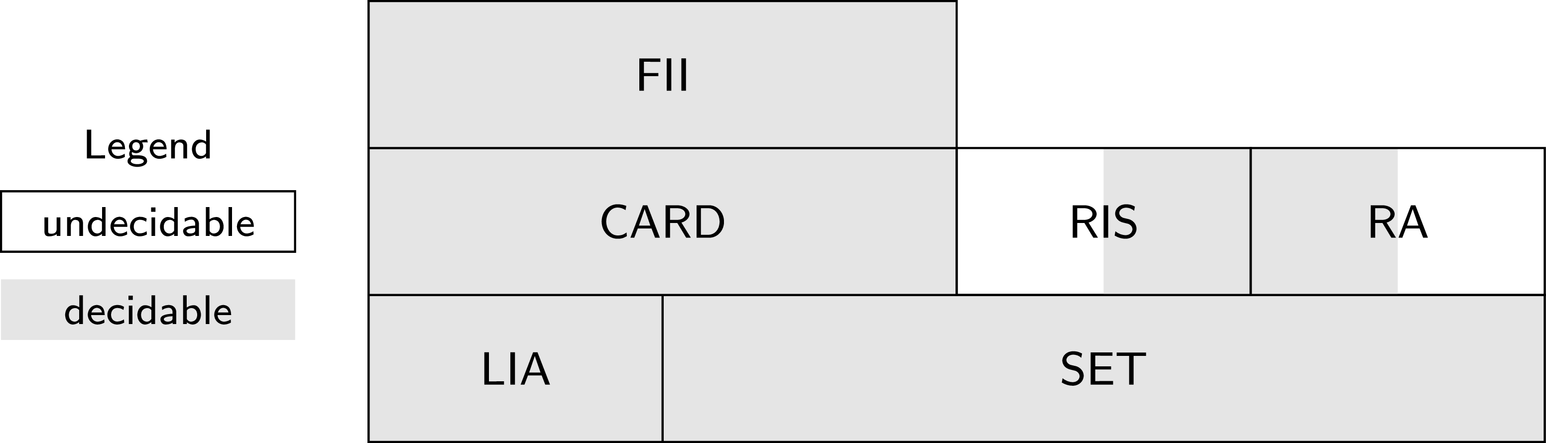
 {log}
{log}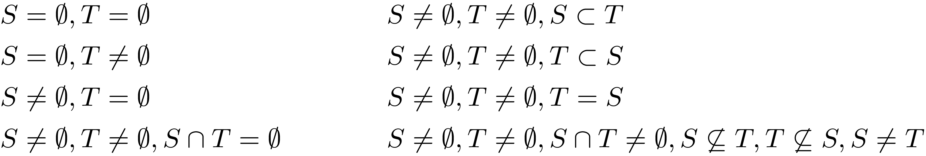
 S∪T
S∪T S∩T
S∩T S∖T
S∖T
 Open access