





1. Introduction
We consider infinite one-dimensional lattices of particles where each particle interacts with every other through pairwise forces. Our main focus is on the existence of solitary travelling wave solutions in generalized Fermi–Pasta–Ulam–Tsingou (FPUT) lattices, where the dynamics are governed by the differential equations
 \begin{equation}
\ddot{x}_j = \sum_{m=1}^\infty \big( \Phi^{\prime}_m(x_{j+m}-x_j) - \Phi^{\prime}_m(x_j-x_{j-m}) \big), \quad j \in \mathbb{Z}.
\end{equation}
\begin{equation}
\ddot{x}_j = \sum_{m=1}^\infty \big( \Phi^{\prime}_m(x_{j+m}-x_j) - \Phi^{\prime}_m(x_j-x_{j-m}) \big), \quad j \in \mathbb{Z}.
\end{equation} Here, 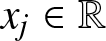 $x_j \in \mathbb{R}$ denotes the position of particle $j$ with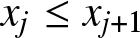 $x_j \leq x_{j+1}$ and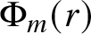 $\Phi_m(r)$ describes the pairwise interaction potentials with the $m^{th}$ neighbour to the left and the right. A typical case are uniform lattices with $\Phi_m(r)= r^{-\alpha}$ for suitable $\alpha \gt 0$. We study solitary travelling waves which satisfy
 \begin{equation}
x_j(t) = \nu j - X(j-ct),
\end{equation}
\begin{equation}
x_j(t) = \nu j - X(j-ct),
\end{equation}where  $\nu$ is a fixed parameter describing an equilibrium distribution of the lattice, $X$ is the wave profile and $c$ the wave speed.
There has been substantial recent interest in the study of travelling waves of long-range FPUT lattices (1.1). A special case is the Calogero–Moser lattice (i.e. for the uniform lattice with 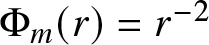 $\Phi_m(r) = r^{-2}$), which defines a completely integrable dynamical system. Formal long-wave calculations and explicit solutions for the Calogero–Moser lattice are given in [Reference Ingimarson and Pego9]. Rigorous small-amplitude, long-wave solutions are given in [Reference Ingimarson and Pego10] and [Reference Akpan and Wright1] through approximations with Benjamin–Ono and Korteweg–de Vries equations, respectively. Initial data approximations by long-wave solutions of Benjamin–Ono equations were studied in [Reference Wright14]. In this paper, we will prove the existence of travelling waves without restriction to small amplitudes for a wide class of long-range interactions.
1.1. Reformulation
Setting 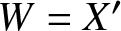 $W = X'$,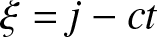 $\xi = j-ct$ and inserting the travelling wave ansatz (1.2) into the dynamic equation (1.1) we get
 \begin{equation}
-c^2 \, {W'}(\xi) = \sum_{m=1}^\infty \big( \Phi^{\prime}_m(\nu m + X(\xi) - X(\xi + m)) - \Phi^{\prime}_m(\nu m - X(\xi) + X(\xi - m) )\big).
\end{equation}
\begin{equation}
-c^2 \, {W'}(\xi) = \sum_{m=1}^\infty \big( \Phi^{\prime}_m(\nu m + X(\xi) - X(\xi + m)) - \Phi^{\prime}_m(\nu m - X(\xi) + X(\xi - m) )\big).
\end{equation} Defining the operator  $A_m$ by convolution with the characteristic function $\chi_{[-m/2,m/2]}$
 \begin{equation}
A_m f(\xi) := \chi_{[-m/2,m/2]} \ast f (\xi) =\int\limits_{-\frac{m}{2}}^{\frac{m}{2}} f(\xi+s) \, {\rm d} s,
\end{equation}
\begin{equation}
A_m f(\xi) := \chi_{[-m/2,m/2]} \ast f (\xi) =\int\limits_{-\frac{m}{2}}^{\frac{m}{2}} f(\xi+s) \, {\rm d} s,
\end{equation}we can express the terms in the sum in (1.3) as
 \begin{align}& \Phi^{\prime}_m\big((\nu m + X(\xi) - X(\xi + m)\big) - \Phi^{\prime}_m\big(\nu m - X(\xi) + X(\xi - m)\big)\nonumber \\
&= \Phi^{\prime}_m\big(\nu m - A_m W (\xi + \frac{m}{2})\big) - \Phi^{\prime}_m\big(\nu m - A_m W (\xi - \frac{m}{2}) \big).\end{align}
\begin{align}& \Phi^{\prime}_m\big((\nu m + X(\xi) - X(\xi + m)\big) - \Phi^{\prime}_m\big(\nu m - X(\xi) + X(\xi - m)\big)\nonumber \\
&= \Phi^{\prime}_m\big(\nu m - A_m W (\xi + \frac{m}{2})\big) - \Phi^{\prime}_m\big(\nu m - A_m W (\xi - \frac{m}{2}) \big).\end{align} Integrating (1.3) with respect to  $\xi$ then yields
 \begin{align}c^2 \, W(x) &= - \sum_{m=1}^\infty \Big( \int_{-\infty}^x \Phi_m'\big(\nu m - A_m W(\xi + \frac{m}{2} ) \big) - \Phi_m'\big(\nu m - A_m W(\xi - \frac{m}{2} ) \big) \, {\rm d} \xi \Big) + \eta \nonumber \\
&= - \sum_{m=1}^\infty \Big( \int_{x-m}^x \Phi_m'\big(\nu m - A_m W(\xi + \frac{m}{2} ) \big) \, {\rm d} \xi \Big) + \eta \nonumber \\
&= - \sum_{m=1}^\infty \Big( \int_{-\frac{m}{2}}^{\frac{m}{2}} \Phi_m'\big(\nu m - A_m W(x + \xi ) \big) \, {\rm d} \xi \Big) + \eta\nonumber \\
&= \sum_{m=1}^\infty \big( A_m (- \Phi_m'(\nu m - A_m W(x) ) ) \big) + \eta,\end{align}
\begin{align}c^2 \, W(x) &= - \sum_{m=1}^\infty \Big( \int_{-\infty}^x \Phi_m'\big(\nu m - A_m W(\xi + \frac{m}{2} ) \big) - \Phi_m'\big(\nu m - A_m W(\xi - \frac{m}{2} ) \big) \, {\rm d} \xi \Big) + \eta \nonumber \\
&= - \sum_{m=1}^\infty \Big( \int_{x-m}^x \Phi_m'\big(\nu m - A_m W(\xi + \frac{m}{2} ) \big) \, {\rm d} \xi \Big) + \eta \nonumber \\
&= - \sum_{m=1}^\infty \Big( \int_{-\frac{m}{2}}^{\frac{m}{2}} \Phi_m'\big(\nu m - A_m W(x + \xi ) \big) \, {\rm d} \xi \Big) + \eta\nonumber \\
&= \sum_{m=1}^\infty \big( A_m (- \Phi_m'(\nu m - A_m W(x) ) ) \big) + \eta,\end{align}due to the structure of the integrand and where  $\eta$ is a suitable constant. We will prove the existence of solutions $(W,c)$ to (1.6) to give the existence of travelling waves of speed $c$ via variational methods.
1.2. Main results
Our approach requires certain properties on the potentials and the norm of  $W$:
$W$:
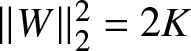
Assumption on  $W$: We will construct our solution by a constrained optimization problem with a constraint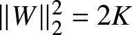 $\|W \|_2^2 = 2K$, where
 \begin{equation}
0 \lt K \lt \frac{\nu^2}{2}
\end{equation}
\begin{equation}
0 \lt K \lt \frac{\nu^2}{2}
\end{equation}is required. We note that this implies
 \begin{equation}
|X(\xi)-X(\xi-m)| = |A_m W|(\xi-\frac{m}{2}) \leq \sqrt{m} \sqrt{2K} \lt \sqrt{m} \nu,
\end{equation}
\begin{equation}
|X(\xi)-X(\xi-m)| = |A_m W|(\xi-\frac{m}{2}) \leq \sqrt{m} \sqrt{2K} \lt \sqrt{m} \nu,
\end{equation}see Lemma 6 below. Hence, we have  $|X(\xi)-X(\xi-m)| \lt \nu m $ and the expressions in (1.3) are well-defined for typical potentials like $r^{-\alpha}$. Indeed, this implies $x_j \lt x_{j+1}$ for the travelling wave solutions.
Assumptions on  $\Phi_m$: For every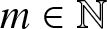 $m \in \mathbb{N}$, the potentials $\Phi_m:(0,\infty)\rightarrow\lbrack0,\infty)$ are in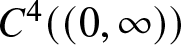 $C^4((0,\infty))$ and satisfy
 \begin{equation}
\Phi_m(s) \geq 0, \quad \Phi_m'(s) \leq 0, \quad \Phi_m^{\prime\prime}(s) \geq 0, \quad \Phi_m^{\prime\prime\prime}(s) \leq 0, \quad \Phi_m^{(4)}(s) \geq 0
\end{equation}
\begin{equation}
\Phi_m(s) \geq 0, \quad \Phi_m'(s) \leq 0, \quad \Phi_m^{\prime\prime}(s) \geq 0, \quad \Phi_m^{\prime\prime\prime}(s) \leq 0, \quad \Phi_m^{(4)}(s) \geq 0
\end{equation}for all  $s \gt 0$. We will require that these inequalities are strict for $m=1$. Furthermore, we assume the global bounds
 \begin{equation}
\sum_{m=1}^\infty {|\Phi_m'(\nu m - \sqrt{2Km}) m|} \lt \infty,
\end{equation}
\begin{equation}
\sum_{m=1}^\infty {|\Phi_m'(\nu m - \sqrt{2Km}) m|} \lt \infty,
\end{equation} \begin{equation}
\sum_{m=1}^\infty {|\Phi_m^{\prime\prime}(\nu m - \sqrt{2Km}) m^2|} \lt \infty,
\end{equation}
\begin{equation}
\sum_{m=1}^\infty {|\Phi_m^{\prime\prime}(\nu m - \sqrt{2Km}) m^2|} \lt \infty,
\end{equation} \begin{equation}
\sum_{m=1}^\infty {|\Phi_m^{\prime\prime}(\nu m) m^\gamma|} \lt \infty
\end{equation}
\begin{equation}
\sum_{m=1}^\infty {|\Phi_m^{\prime\prime}(\nu m) m^\gamma|} \lt \infty
\end{equation} $\gamma\in(5/2, 3)$ is fixed. Here, we use (1.7) to ensure $\nu m-\sqrt{2Km} \gt 0$.
Lemma 1. Let  $\Phi_m(r) = r^{-\alpha}$ with $\alpha \gt \frac32$, then $\Phi_m {, m \in \mathbb{N},}$ satisfies the assumptions (1.9), (1.10a), (1.10b) and (1.10c) listed above.
Proof. This is a direct calculation.
We can now state the main result of this paper.
Theorem 2 (Main Result)
Under the assumptions on  $\Phi_m$ and $K$, there exists a one-parameter family of solutions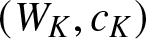 $(W_K,c_K)$ of (1.6) with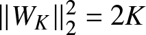 $\|W_K\|^2_2= 2K$.
(1) The result can be expressed for the specific choice of the typical uniform lattices by using Lemma 1, i.e. for given $\nu \gt 0$ and
$\alpha \gt 3/2$, there exists a family of travelling waves of (1.1) for
$\Phi_m(r)=r^{-\alpha}$ with
$\|W\|_2^2=2K$ for each
$K$ with
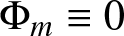
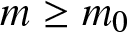
$0 \lt K \lt \nu^2/2$. The result also implies an existence result for lattices with repulsive finite-range forces, i.e.
$\Phi_m \equiv 0$ for
$m \geq m_0$ for some fixed
$m_0$.
$\nu \gt 0$ and
$\alpha \gt 3/2$, there exists a family of travelling waves of (1.1) for
$\Phi_m(r)=r^{-\alpha}$ with
$\|W\|_2^2=2K$ for each
$K$ with
$0 \lt K \lt \nu^2/2$. The result also implies an existence result for lattices with repulsive finite-range forces, i.e.
$\Phi_m \equiv 0$ for
$m \geq m_0$ for some fixed
$m_0$.(2) The high-energy limit for
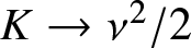
$K \to \nu^2/2$ is described in detail below for the potential
$r^{-\alpha}$. The behaviour is analogous to the standard FPUT case as analysed, e.g. in [Reference Herrmann and Matthies5]. In Section 3, we establish that
$W_K$ converges to an indicator function and that
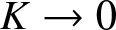
$c_K \to \infty$.(3) For
$K \to 0$, it can be expected that the travelling waves approach the long-wave solutions as given in [Reference Ingimarson and Pego10] and [Reference Akpan and Wright1], the rigorous limit in our variational setting is left out for reasons of brevity. A parallel, entirely variational analysis is done in [Reference Herrmann and Matthies7] for general related convolution operators for a long-wave limit approaching the KdV equation.









1.3. Further related results
Early work on variational proofs for the existence of travelling waves are [Reference Friesecke and Wattis3] and [Reference Filip and Venakides2]. There is a comprehensive overview on travelling waves in FPUT including models with next-nearest neighbours interactions by Vainchtein [Reference Vainchtein13]. Finite-range interactions, i.e. 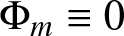 $\Phi_m \equiv 0$ for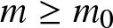 $m \geq m_0$ for some fixed $m_0$ were studied via a long-wave KdV approach in [Reference Herrmann and Mikikits-Leitner8], which was adapted to the infinite range case in [Reference Ingimarson and Pego10] and [Reference Akpan and Wright1] to get small-amplitude, long-wave travelling waves. We note that Ingimarson and Pego [Reference Ingimarson and Pego10] show the existence of travelling waves for the setting of Lemma 1 for the range of parameters $4/3 \lt \alpha \lt 3$. They encounter different qualitative behaviour for those with $\alpha \in (4/3,3/2)$ in that the Hamiltonian energy of the waves is not monotonically increasing in the wave speed; this is in contrast to what can be expected for waves constructed by our variational approach for small $K$.
$K$.
For finite-range interaction, variational methods gave the existence of travelling waves of finite size in [Reference Herrmann and Matthies6] and [Reference Pankov11]. Our approach uses a variational principle similar to the existence proof for FPUT travelling waves in [Reference Herrmann4]. Similar adaptations of [Reference Herrmann4] were made in [Reference Herrmann and Matthies6] for peridynamical media (and finite-range FPUT) and in [Reference Herrmann and Matthies7] to a general convolution setting; see these papers also for discussions of other variational methods to construct solutions of FPUT.
Plan of the paper: We introduce the variational principle in Subsection 2.1 on a suitable cone of unimodal functions. The existence of maximizers is shown in Subsection 2.2 using a concentration compactness argument. The proof of the main theorem is given in Subsection 2.3. In Section 3, we discuss the asymptotic behaviour for high-energy waves, i.e. for 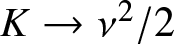 $K \to \nu^2/2$.
2. Construction of travelling wave solutions
The proof of existence follows the variational approach of [Reference Herrmann and Matthies7], where nonlinear, nonlocal eigenvalue problems of a form that include nearest-neighbour FPUT chains are analysed. Similar methods were adapted in [Reference Herrmann and Matthies6] for peridynamical media which contained the more general FPUT case  $\Phi_1=\Phi_2=\ldots=\Phi_M$ and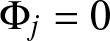 $\Phi_j=0 $ for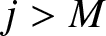 $j \gt M$.
While the overall structure of the argument follows the approach of [Reference Herrmann and Matthies7], the present setting introduces substantial new analytical difficulties. In contrast to the finite-range interactions considered there, each particle in our model interacts with every other particle. As a consequence, several steps of the variational analysis require nontrivial modifications. In particular, it becomes necessary to establish the well-posedness of certain infinite series, such as the series  $\mathcal{P}$ defined in the next subsection, a question that does not arise in [Reference Herrmann and Matthies7] or related finite-range models. While some proofs of lemmas only require minor modifications, we provide all proofs to keep the exposition self-contained.
2.1. Variational setting
Following the variational method that is described in [Reference Herrmann and Matthies7], we first define the potential and kinetic energy of  $W$ by
 \begin{equation}
\mathcal{P}(W) := \int\limits_{\mathbb{R}} \sum_{m=1}^\infty \Psi_m ( A_m W(s)) \, {\rm d}s, \qquad \mathcal{K}(W) := \frac12 \int\limits_{\mathbb{R}} \big( W(s) \big)^2 \, {\rm d}s,
\end{equation}
\begin{equation}
\mathcal{P}(W) := \int\limits_{\mathbb{R}} \sum_{m=1}^\infty \Psi_m ( A_m W(s)) \, {\rm d}s, \qquad \mathcal{K}(W) := \frac12 \int\limits_{\mathbb{R}} \big( W(s) \big)^2 \, {\rm d}s,
\end{equation}respectively. Here,  $\Psi_m :[0,\nu m) \to [0,\infty)$ is obtained by correcting the first two terms of the Taylor approximation of $\Phi_m$ around $\nu m$ and is given by
 \begin{equation}
\Psi_m(r) := \Phi_m(\nu m - r) - \Phi_m(\nu m) + \Phi_m'(\nu m)r.
\end{equation}
\begin{equation}
\Psi_m(r) := \Phi_m(\nu m - r) - \Phi_m(\nu m) + \Phi_m'(\nu m)r.
\end{equation} We constrain our optimization to cones. Here,  $\mathcal{C}$ is the convex cone given by all square integrable, even, unimodal and nonnegative functions, i.e.
 \begin{equation}
\mathcal{C} := \overline{\{W \in C_c^\infty(\mathbb{R}) \mid W(x) = W(-x) \geq 0 \quad \text{and} \quad {W'(x) = -W'(-x)} \leq 0 \quad \text{for all } x \geq 0 \}},
\end{equation}
\begin{equation}
\mathcal{C} := \overline{\{W \in C_c^\infty(\mathbb{R}) \mid W(x) = W(-x) \geq 0 \quad \text{and} \quad {W'(x) = -W'(-x)} \leq 0 \quad \text{for all } x \geq 0 \}},
\end{equation}where the overline denote the  $\mathsf{L}^2(\mathbb{R})$ closure. Due to convexity, $\mathcal{C}$ is also closed under weak convergence in $\mathsf{L}^2(\mathbb{R})$. Then for every given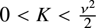 $0 \lt K \lt \frac{\nu^2}{2}$ we define the cone
 \begin{equation}
\mathcal{C}_K := \{W \in \mathcal{C} \mid \mathcal{K}(W) = K\}.
\end{equation}
\begin{equation}
\mathcal{C}_K := \{W \in \mathcal{C} \mid \mathcal{K}(W) = K\}.
\end{equation}We note briefly that ‘unimodal’ functions are also called ‘bell-shaped’ in parts of the travelling wave literature, see e.g. [Reference Stefanov and Kevrekidis12].
The general idea is to find a converging sequence 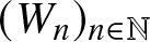 $(W_n)_{n\in\mathbb{N}}$ of functions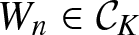 $W_n \in \mathcal{C}_K$ that maximizes the potential energy such that its limit $W_{\infty}$ is a solution to the travelling wave problem. First, we prove some auxiliary results and ensure that the potential energy $\mathcal{P}$ is indeed well-defined. We observe some further global bounds.
Remark 4. The bound in (1.10a) implies with 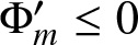 $\Phi_m' \leq 0$ and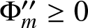 $\Phi_m^{\prime\prime} \geq 0$ the global estimate
 \begin{equation}
\sum_{m=1}^\infty {|\Phi_m'(\nu m) m|} \lt \infty.
\end{equation}
\begin{equation}
\sum_{m=1}^\infty {|\Phi_m'(\nu m) m|} \lt \infty.
\end{equation} The corrected potentials  $\Psi_m$ as in (2.2) have a minimum at $r=0$. We collect further properties in the next lemma.
Lemma 5. For every 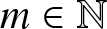 $m \in \mathbb{N}$, the potential $\Psi_m$ satisfies
 \begin{align}
\Psi_m(0) = \Psi_m'(0) = 0, \quad \Psi_m^{\prime\prime}(0) = \Phi_m^{\prime\prime}(\nu m) \geq 0
\end{align}
\begin{align}
\Psi_m(0) = \Psi_m'(0) = 0, \quad \Psi_m^{\prime\prime}(0) = \Phi_m^{\prime\prime}(\nu m) \geq 0
\end{align}and
 \begin{equation}
\!\!\!\!\!\!\!\!\!\!\!\!\!\!\!\!\!\!\!\!\!\!\!\!\!\!\!\!\!\!\!\!\!\!\!\!\!\!\!\!\!\!\!\!\!\!\!\!\!\!\!\!\!\!\!\!\!\!\!\!\!\!\!\!\!\!\!\!\!\!\!\!\!\!\!\Psi_m(r) \geq 0,
\end{equation}
\begin{equation}
\!\!\!\!\!\!\!\!\!\!\!\!\!\!\!\!\!\!\!\!\!\!\!\!\!\!\!\!\!\!\!\!\!\!\!\!\!\!\!\!\!\!\!\!\!\!\!\!\!\!\!\!\!\!\!\!\!\!\!\!\!\!\!\!\!\!\!\!\!\!\!\!\!\!\!\Psi_m(r) \geq 0,
\end{equation} \begin{equation}
\!\!\!\!\!\!\!\Psi_m'(r) = -\Phi_m'(\nu m - r) + {\Phi_m'}(\nu m) \geq 0,
\end{equation}
\begin{equation}
\!\!\!\!\!\!\!\Psi_m'(r) = -\Phi_m'(\nu m - r) + {\Phi_m'}(\nu m) \geq 0,
\end{equation} \begin{equation}
\!\!\!\!\!\!\!\!\!\!\!\!\!\!\!\!\!\!\!\!\!\!\!\!\!\!\!\!\!\!\!\!\!\!\!\!\!\!\!\!\!\Psi_m^{\prime\prime}(r) = \Phi_m^{\prime\prime}(\nu m - r) \geq 0
\end{equation}
\begin{equation}
\!\!\!\!\!\!\!\!\!\!\!\!\!\!\!\!\!\!\!\!\!\!\!\!\!\!\!\!\!\!\!\!\!\!\!\!\!\!\!\!\!\Psi_m^{\prime\prime}(r) = \Phi_m^{\prime\prime}(\nu m - r) \geq 0
\end{equation} for all 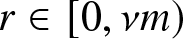 $r \in [0,\nu m)$.
Proof. These are direct consequences of the definition of  $\Psi_m$ and the assumptions on $\Phi_m$ and its derivatives, e.g. a Taylor expanding of $\Phi_m$ around $\nu m$ reveals
 \begin{equation}
\Phi_m(\nu m -r) = \Phi_m(\nu m) - \Phi_m'(\nu m)r + \Phi_m^{\prime\prime}(\nu m - \theta r)\frac{r^2}{2!}
\end{equation}
\begin{equation}
\Phi_m(\nu m -r) = \Phi_m(\nu m) - \Phi_m'(\nu m)r + \Phi_m^{\prime\prime}(\nu m - \theta r)\frac{r^2}{2!}
\end{equation}with 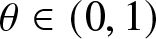 $\theta \in (0,1)$, which implies
 \begin{equation}
\Psi_m(r) = \Phi_m^{\prime\prime}(\nu m - \theta r)\frac{r^2}{2!} \geq 0.
\end{equation}
\begin{equation}
\Psi_m(r) = \Phi_m^{\prime\prime}(\nu m - \theta r)\frac{r^2}{2!} \geq 0.
\end{equation} Next, we state properties of the convolution operator applied to elements of the cone  $\mathcal{C}_K$.
Lemma 6. Let 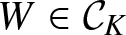 $W \in \mathcal{C}_K$ and $m \in \mathbb{N}$, then $0 \leq A_m W(s) \leq \sqrt{2Km} $ for all $s \in \mathbb{R}$.
Proof. The nonnegativity of 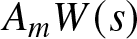 $A_m W(s)$ is trivial due to the definition of $A_m$ and $W$ being nonnegative. Young’s convolution inequality yields
 \begin{equation}
A_m W(s) \leq \|A_m W\|_{\infty} = \| \chi_{[-m/2,m/2]} \ast W \|_{\infty} \leq \| \chi_{[-m/2,m/2]} \|_2 \| W \|_{2} = \sqrt{m} \sqrt{2K}.
\end{equation}
\begin{equation}
A_m W(s) \leq \|A_m W\|_{\infty} = \| \chi_{[-m/2,m/2]} \ast W \|_{\infty} \leq \| \chi_{[-m/2,m/2]} \|_2 \| W \|_{2} = \sqrt{m} \sqrt{2K}.
\end{equation} Now we are in the position to show that  $\mathcal{P}(W)$ is finite for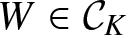 $W \in \mathcal{C}_K$.
Lemma 7. The potential energy  $\mathcal{P}$ is well-defined for all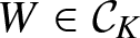 $W \in \mathcal{C}_K$.
Proof. Lemmas 5 and 6 imply for some 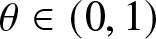 $\theta \in (0,1)$
 \begin{equation}
0 \leq \Psi_m(A_mW(s)) = {\Phi_m^{\prime\prime}}(\nu m - \theta A_m W)\frac{(A_m W(s))^2}{2} \leq \Phi_m^{\prime\prime}\big(\nu m - \sqrt{2Km}\big) \frac{(A_mW(s))^2}{2},
\end{equation}
\begin{equation}
0 \leq \Psi_m(A_mW(s)) = {\Phi_m^{\prime\prime}}(\nu m - \theta A_m W)\frac{(A_m W(s))^2}{2} \leq \Phi_m^{\prime\prime}\big(\nu m - \sqrt{2Km}\big) \frac{(A_mW(s))^2}{2},
\end{equation}using in the last step that  $ {\Phi_m^{\prime\prime}}$ is monotonically decreasing. Note that the expressions $\Phi_m^{\prime\prime}(\nu m - \sqrt{2Km})$ are well-defined for all $m \in \mathbb{N}$ due to the condition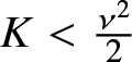 $K \lt \frac{\nu^2}{2}$. With $C_{m,K} := \frac12 \Phi_m^{\prime\prime}\big(\nu m - \sqrt{2Km}\big)$, Hölder’s inequality and Fubini’s theorem we then get
 \begin{align}
\int\limits_{\mathbb{R}} &\Psi_m(A_mW(s)) \, {\rm d}s \leq C_{m,K} \int\limits_{\mathbb{R}} ( A_mW(s) )^2 \,{\rm d}s
= C_{m,K} \int\limits_{\mathbb{R}} \Big[ \int\limits_{-\frac{m}{2}}^{\frac{m}{2}} W(s+\tau) \, {\rm d}\tau \Big]^2 \,{\rm d}s \nonumber \\
&\leq C_{m,K} \int\limits_{\mathbb{R}} \Big[m \, \int\limits_{-\frac{m}{2}}^{\frac{m}{2}} W^2(s+\tau) \, {\rm d}\tau \Big] \,{\rm d}s= m \, C_{m,K} \int\limits_{-\frac{m}{2}}^{\frac{m}{2}} \int\limits_{\mathbb{R}} W^2(s+\tau) \, {\rm d}s \,{\rm d}\tau\nonumber \\
&= m \, C_{m,K} \int\limits_{-\frac{m}{2}}^{\frac{m}{2}} 2K \,{\rm d}\tau
= 2K m^2 C_{m,K}.
\end{align}
\begin{align}
\int\limits_{\mathbb{R}} &\Psi_m(A_mW(s)) \, {\rm d}s \leq C_{m,K} \int\limits_{\mathbb{R}} ( A_mW(s) )^2 \,{\rm d}s
= C_{m,K} \int\limits_{\mathbb{R}} \Big[ \int\limits_{-\frac{m}{2}}^{\frac{m}{2}} W(s+\tau) \, {\rm d}\tau \Big]^2 \,{\rm d}s \nonumber \\
&\leq C_{m,K} \int\limits_{\mathbb{R}} \Big[m \, \int\limits_{-\frac{m}{2}}^{\frac{m}{2}} W^2(s+\tau) \, {\rm d}\tau \Big] \,{\rm d}s= m \, C_{m,K} \int\limits_{-\frac{m}{2}}^{\frac{m}{2}} \int\limits_{\mathbb{R}} W^2(s+\tau) \, {\rm d}s \,{\rm d}\tau\nonumber \\
&= m \, C_{m,K} \int\limits_{-\frac{m}{2}}^{\frac{m}{2}} 2K \,{\rm d}\tau
= 2K m^2 C_{m,K}.
\end{align} Substituting the results into the formula for  $\mathcal{P}$ and using Fubini’s theorem, we get
 \begin{align}\mathcal{P}(W) &= \int\limits_{\mathbb{R}} \sum_{m=1}^\infty \Psi_m ( A_m W(s)) \, {\rm d}s
= \sum_{m=1}^\infty \int\limits_{\mathbb{R}} \Psi_m ( A_m W(s)) \, {\rm d}s \nonumber\\
&\leq \sum_{m=1}^\infty 2K m^2 C_{m,K}
= \sum_{m=1}^\infty K m^2 \Phi_m^{\prime\prime}(\nu m - \sqrt{2Km}) \lt \infty,\end{align}
\begin{align}\mathcal{P}(W) &= \int\limits_{\mathbb{R}} \sum_{m=1}^\infty \Psi_m ( A_m W(s)) \, {\rm d}s
= \sum_{m=1}^\infty \int\limits_{\mathbb{R}} \Psi_m ( A_m W(s)) \, {\rm d}s \nonumber\\
&\leq \sum_{m=1}^\infty 2K m^2 C_{m,K}
= \sum_{m=1}^\infty K m^2 \Phi_m^{\prime\prime}(\nu m - \sqrt{2Km}) \lt \infty,\end{align}where the last step follows by assumption (1.10b).
We will consider a maximizing sequence 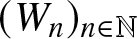 $(W_n)_{n\in\mathbb{N}}$. Such sequences can be constructed using an improvement operator
 \begin{equation}
\mathcal{T}(W) := \mu(W)\partial\mathcal{P}(W)
\end{equation}
\begin{equation}
\mathcal{T}(W) := \mu(W)\partial\mathcal{P}(W)
\end{equation}with
 \begin{equation}
\mu(W) := \frac{\|W\|_2}{\|\partial \mathcal{P}(W)\|_2} \quad \text{and} \quad \partial \mathcal{P}(W) = \sum_{m=1}^\infty A_m \Psi_m'(A_m W).
\end{equation}
\begin{equation}
\mu(W) := \frac{\|W\|_2}{\|\partial \mathcal{P}(W)\|_2} \quad \text{and} \quad \partial \mathcal{P}(W) = \sum_{m=1}^\infty A_m \Psi_m'(A_m W).
\end{equation} We will not use an explicitly constructed sequence, but invariance properties of the cone  $\mathcal{C}_K$ will be relevant.
Lemma 8. The gradient  $\partial\mathcal{P}$ is well-defined for all $W \in \mathcal{C}_K$.
Proof. Let 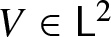 $V \in \mathsf{L}^2$ be fixed. Analogous to the computations in (2.14) follows
 \begin{equation}
\|A_m V\|_2 \leq m \| V \|_2.
\end{equation}
\begin{equation}
\|A_m V\|_2 \leq m \| V \|_2.
\end{equation} In addition, a Taylor expansion of  $\Phi_m'$ and Young’s convolution inequality yield the estimate
 \begin{align}\|\Psi_m'&(A_m W) \|_2 = \Big( \int\limits_{\mathbb{R}} \big( \Psi_m'(A_m W(s) ) \big)^2 \, {\rm d} s \Big)^{\frac12} \nonumber \\
&= \Big( \int\limits_{\mathbb{R}} \big( \Phi_m'(\nu m) - \Phi_m'(\nu m - A_m W(s) ) \big)^2 \, {\rm d} s \Big)^{\frac12} \nonumber \\
&\leq \Big( \int\limits_{\mathbb{R}} \big( \Phi_m^{\prime\prime}(\nu m - \sqrt{2Km} ) (A_m W(s) )^2 {\rm d} s \Big)^{\frac12} \nonumber \\
&= \Phi_m^{\prime\prime}(\nu m - \sqrt{2Km} ) \|A_m W\|_2 \leq \Phi_m^{\prime\prime}(\nu m- \sqrt{2Km}) \sqrt{2K} m.\end{align}
\begin{align}\|\Psi_m'&(A_m W) \|_2 = \Big( \int\limits_{\mathbb{R}} \big( \Psi_m'(A_m W(s) ) \big)^2 \, {\rm d} s \Big)^{\frac12} \nonumber \\
&= \Big( \int\limits_{\mathbb{R}} \big( \Phi_m'(\nu m) - \Phi_m'(\nu m - A_m W(s) ) \big)^2 \, {\rm d} s \Big)^{\frac12} \nonumber \\
&\leq \Big( \int\limits_{\mathbb{R}} \big( \Phi_m^{\prime\prime}(\nu m - \sqrt{2Km} ) (A_m W(s) )^2 {\rm d} s \Big)^{\frac12} \nonumber \\
&= \Phi_m^{\prime\prime}(\nu m - \sqrt{2Km} ) \|A_m W\|_2 \leq \Phi_m^{\prime\prime}(\nu m- \sqrt{2Km}) \sqrt{2K} m.\end{align}In summary, using the Cauchy–Schwarz inequality, we obtain
 \begin{align}\langle \partial &\mathcal{P}(W), V \rangle = \sum_{m=1}^\infty \langle A_m \Psi_m'(A_m W), V \rangle {\leq} \sum_{m=1}^\infty \|\Psi_m'(A_m W) \|_2 \|A_m V\|_2 \nonumber \\
&\leq \sum_{m=1}^\infty \sqrt{2K} \|V\|_2 \Phi_m^{\prime\prime}(\nu m - \sqrt{2Km}) m^2 \leq C \|V\|_2\end{align}
\begin{align}\langle \partial &\mathcal{P}(W), V \rangle = \sum_{m=1}^\infty \langle A_m \Psi_m'(A_m W), V \rangle {\leq} \sum_{m=1}^\infty \|\Psi_m'(A_m W) \|_2 \|A_m V\|_2 \nonumber \\
&\leq \sum_{m=1}^\infty \sqrt{2K} \|V\|_2 \Phi_m^{\prime\prime}(\nu m - \sqrt{2Km}) m^2 \leq C \|V\|_2\end{align}by (1.10b). Hence 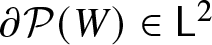 $\partial \mathcal{P}(W) \in \mathsf{L}^2$ as required.
Lemma 9. Let  $W \in \mathcal{C}_K$, then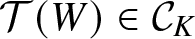 $\mathcal{T}(W) \in \mathcal{C}_K$.
Proof. Let  $W \in \mathcal{C}_K$. Using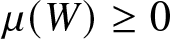 $\mu(W) \geq 0$ and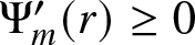 $\Psi_m'(r) \geq 0$ for all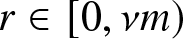 $ {r \in [0, \nu m)}$ we get the nonnegativity of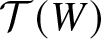 $\mathcal{T}(W)$ via
 \begin{align}W \geq 0 &\Rightarrow A_m W \geq 0 \Rightarrow \Psi_m'(A_m W) \geq 0 \Rightarrow A_m \Psi_m'(A_m W) \geq 0 \nonumber \\
&\Rightarrow \sum_{m=1}^\infty A_m \Psi_m'(A_m W) \geq 0 \Rightarrow \mathcal{T}(W) \geq 0.\end{align}
\begin{align}W \geq 0 &\Rightarrow A_m W \geq 0 \Rightarrow \Psi_m'(A_m W) \geq 0 \Rightarrow A_m \Psi_m'(A_m W) \geq 0 \nonumber \\
&\Rightarrow \sum_{m=1}^\infty A_m \Psi_m'(A_m W) \geq 0 \Rightarrow \mathcal{T}(W) \geq 0.\end{align} Furthermore, the evenness of  $W$ gives the evenness of $A_m W$, and hence $\Psi_m'(A_m W)$ is even as well. The repeated application of $A_m$ and the multiplication with the scalar $\mu(W)$ does not change this property and thus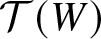 $\mathcal{T}(W)$ is even. From both the evenness and unimodality of $W$, we deduce the unimodality of $A_m W$ from
 \begin{equation}
A_m W(x) = \int\limits_{-\frac{m}{2}}^{\frac{m}{2}} W(x+s) \, {\rm d}s \leq \int\limits_{-\frac{m}{2}}^{\frac{m}{2}} W(s) \, {\rm d}s = A_m W(0)
\end{equation}
\begin{equation}
A_m W(x) = \int\limits_{-\frac{m}{2}}^{\frac{m}{2}} W(x+s) \, {\rm d}s \leq \int\limits_{-\frac{m}{2}}^{\frac{m}{2}} W(s) \, {\rm d}s = A_m W(0)
\end{equation}for all  $x \in \mathbb{R}$. $\Psi_m'$ is monotonically increasing, hence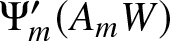 $\Psi_m'(A_mW)$ is unimodal. It follows that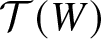 $\mathcal{T}(W)$ is unimodal.
We conclude the proof with the observation  $ {\| \mathcal{T}(W) \|_2^2 = \| W \|_2^2} = 2K$.
The operator  $\mathcal{T}$ strictly increases the potential energy unless we have already a travelling wave solution.
Lemma 10. Let  $W \in \mathcal{C}_K$, then $\mathcal{P}(\mathcal{T}(W)) \geq \mathcal{P}(W)$. Moreover, equality holds if and only if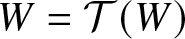 $W = \mathcal{T}(W)$, i.e. $W$ satisfies (1.6) with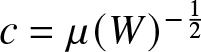 $c = \mu(W)^{-\frac12}$.
Proof.  $\Psi_m^{\prime\prime}(r) \geq 0$ implies that $\mathcal{P}$ is convex and hence,
 \begin{equation}
\mathcal{P}(V) - \mathcal{P}(W) \geq \langle \partial \mathcal{P}(W), V-W \rangle
\end{equation}
\begin{equation}
\mathcal{P}(V) - \mathcal{P}(W) \geq \langle \partial \mathcal{P}(W), V-W \rangle
\end{equation}holds for all  $V,W \in \mathsf{L}^2(\mathbb{R})$. This result and Lemma 9 yield
 \begin{align}\mathcal{P}(\mathcal{T}(W)) - \mathcal{P}(W) &\geq \langle \partial \mathcal{P}(W), \mathcal{T}(W)-W \rangle
= \frac{\langle \mathcal{T}(W), \mathcal{T}(W)-W \rangle }{\mu(W)}
\nonumber \\
&= \frac{\|\mathcal{T}(W)\|_2^2 - 2 \langle\mathcal{T}(W),W\rangle + \|W\|_2^2}{2\mu(W)}
= \frac{\| {\mathcal{T}}(W)-W\|_2^2}{2\mu(W)}.\end{align}
\begin{align}\mathcal{P}(\mathcal{T}(W)) - \mathcal{P}(W) &\geq \langle \partial \mathcal{P}(W), \mathcal{T}(W)-W \rangle
= \frac{\langle \mathcal{T}(W), \mathcal{T}(W)-W \rangle }{\mu(W)}
\nonumber \\
&= \frac{\|\mathcal{T}(W)\|_2^2 - 2 \langle\mathcal{T}(W),W\rangle + \|W\|_2^2}{2\mu(W)}
= \frac{\| {\mathcal{T}}(W)-W\|_2^2}{2\mu(W)}.\end{align} It follows that  $\mathcal{P}(\mathcal{T}(W)) \geq \mathcal{P}(W)$ and equality holds if and only if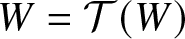 $W = \mathcal{T}(W)$. Finally, if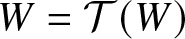 $W = \mathcal{T}(W)$, we note
 \begin{align}
W = \mathcal{T}(W) &= \mu(W)\partial \mathcal{P}(W)
= \mu(W) \sum_{m=1}^\infty A_m\Psi_m'(A_m W) \nonumber \\
&= \mu(W) \sum_{m=1}^\infty A_m \big( -\Phi_m'(\nu m - A_m W) + \Phi_m'(\nu m) \big) \nonumber \\
&= \mu(W) \sum_{m=1}^\infty A_m \big( -\Phi_m'(\nu m - A_m W) \big) + \mu(W) \sum_{m=1}^\infty A_m \big( \Phi_m'(\nu m) \big),
\end{align}
\begin{align}
W = \mathcal{T}(W) &= \mu(W)\partial \mathcal{P}(W)
= \mu(W) \sum_{m=1}^\infty A_m\Psi_m'(A_m W) \nonumber \\
&= \mu(W) \sum_{m=1}^\infty A_m \big( -\Phi_m'(\nu m - A_m W) + \Phi_m'(\nu m) \big) \nonumber \\
&= \mu(W) \sum_{m=1}^\infty A_m \big( -\Phi_m'(\nu m - A_m W) \big) + \mu(W) \sum_{m=1}^\infty A_m \big( \Phi_m'(\nu m) \big),
\end{align}providing a solution to (1.6) with
 \begin{equation}
c = \mu(W)^{-\frac12}
\end{equation}
\begin{equation}
c = \mu(W)^{-\frac12}
\end{equation}and
 \begin{equation}
\eta = \sum_{m=1}^\infty A_m \Phi_m'(\nu m)= \sum_{m=1}^\infty m \Phi_m'(\nu m).
\end{equation}
\begin{equation}
\eta = \sum_{m=1}^\infty A_m \Phi_m'(\nu m)= \sum_{m=1}^\infty m \Phi_m'(\nu m).
\end{equation}2.2. Existence of maximizers
It is our goal to show that every maximizing sequence for  $\mathcal{P}$ in $\mathcal{C}_K$ admits a strongly convergent subsequence. This will complete the existence proof of a maximizer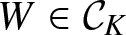 $W \in \mathcal{C}_K$, which is then a solution of (1.6). For this purpose, we define – based on the quantities in [Reference Herrmann and Matthies7] – the quantities
 \begin{equation}
P(K) := \sup\limits_{W \in \mathcal{C}_K} \mathcal{P}(W), \qquad Q(K) := \sup\limits_{W \in \mathcal{C}_K} \mathcal{Q}(W)
\end{equation}
\begin{equation}
P(K) := \sup\limits_{W \in \mathcal{C}_K} \mathcal{P}(W), \qquad Q(K) := \sup\limits_{W \in \mathcal{C}_K} \mathcal{Q}(W)
\end{equation}with
 \begin{equation}
\mathcal{Q}(W) := \frac{1}{2} \int\limits_{\mathbb{R}} \sum_{m=1}^\infty \Phi_m^{\prime\prime}(\nu m) ( A_m W(s) )^2 \,{\rm d}s.
\end{equation}
\begin{equation}
\mathcal{Q}(W) := \frac{1}{2} \int\limits_{\mathbb{R}} \sum_{m=1}^\infty \Phi_m^{\prime\prime}(\nu m) ( A_m W(s) )^2 \,{\rm d}s.
\end{equation} Note that  $\mathcal{Q}$ is the quadratic term of $\mathcal{P}$ when Taylor expanding $\Psi_m$ around $0$ in the definition of $\mathcal{P}$ and recalling $\Psi_m^{\prime\prime}(0) = \Phi_m^{\prime\prime}(\nu m)$. The subsequent lemma quantifies $Q(K)$ before we prove in Lemma 12 that $P(K)$ is strictly greater than $Q(K)$, implying that the super-quadratic terms in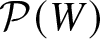 $\mathcal{P}(W)$ play a significant role.
Lemma 11. For all  $K \gt 0$, $Q(K) = \sum_{m=1}^\infty \Phi_m^{\prime\prime}(\nu m) K m^2$ holds.
Proof. Using Hölder’s inequality and Fubini’s theorem in the same way as in the proof of Lemma 7, we obtain an upper bound
 \begin{equation}
Q(K) \leq \sum_{m=1}^\infty \Phi_m^{\prime\prime}(\nu m) K m^2.
\end{equation}
\begin{equation}
Q(K) \leq \sum_{m=1}^\infty \Phi_m^{\prime\prime}(\nu m) K m^2.
\end{equation} Now, we consider a family of test functions to get matching lower bounds. For a parameter 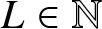 $L \in \mathbb{N}$ such that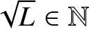 $\sqrt{L} \in \mathbb{N}$, we define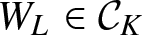 $W_L \in \mathcal{C}_K$ by
 \begin{equation}
W_L(x) := \sqrt{\frac{K}{L}}\, \chi_{[-L,L]}(x)
\end{equation}
\begin{equation}
W_L(x) := \sqrt{\frac{K}{L}}\, \chi_{[-L,L]}(x)
\end{equation}and note that for all  $m \leq 2L$ (and in particular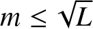 $m \leq \sqrt{L}$) we have
 \begin{equation}
A_m W_L(\xi) = \begin{cases}
\sqrt{\frac{K}{L}}\,m \, &\text{if}\,\, 0 \leq |\xi| \leq L - \frac{m}{2}, \\
\sqrt{\frac{K}{L}}\, (L - ( {|\xi|}-\frac{m}{2})) \, &\text{if}\,\, L - \frac{m}{2} \lt |\xi| \leq L + \frac{m}{2},\\
0 \, &\text{if}\,\, |\xi| \gt L+\frac{m}{2}.
\end{cases}
\end{equation}
\begin{equation}
A_m W_L(\xi) = \begin{cases}
\sqrt{\frac{K}{L}}\,m \, &\text{if}\,\, 0 \leq |\xi| \leq L - \frac{m}{2}, \\
\sqrt{\frac{K}{L}}\, (L - ( {|\xi|}-\frac{m}{2})) \, &\text{if}\,\, L - \frac{m}{2} \lt |\xi| \leq L + \frac{m}{2},\\
0 \, &\text{if}\,\, |\xi| \gt L+\frac{m}{2}.
\end{cases}
\end{equation}With (2.32), it follows
 \begin{align}
\mathcal{Q}(W_L)
&= \frac12 \sum_{m=1}^\infty \Phi_m^{\prime\prime}(\nu m)
\int_{\mathbb{R}} (A_m W_L(s))^2 \,{\rm d}s\ge \frac12 \sum_{m=1}^{L}
\Phi_m^{\prime\prime}(\nu m)
\int_{-(L-\frac{m}{2})}^{L-\frac{m}{2}}
(A_m W_L(s))^2 \,{\rm d}s \nonumber\\
&= \frac12 \sum_{m=1}^{L}
\Phi_m^{\prime\prime}(\nu m)\,
\frac{K}{L}m^2(2L-m) = \sum_{m=1}^{L}
\Phi_m^{\prime\prime}(\nu m)K m^2
\Bigl(1-\frac{m}{2L}\Bigr) \nonumber\\
&\ge \sum_{m=1}^{\sqrt{L}}
\Phi_m^{\prime\prime}(\nu m)K m^2
\Bigl(1-\frac{m}{2L}\Bigr)\ge \sum_{m=1}^{\sqrt{L}}
\Phi_m^{\prime\prime}(\nu m)K m^2
\Bigl(1-\frac{1}{2\sqrt{L}}\Bigr).
\end{align}
\begin{align}
\mathcal{Q}(W_L)
&= \frac12 \sum_{m=1}^\infty \Phi_m^{\prime\prime}(\nu m)
\int_{\mathbb{R}} (A_m W_L(s))^2 \,{\rm d}s\ge \frac12 \sum_{m=1}^{L}
\Phi_m^{\prime\prime}(\nu m)
\int_{-(L-\frac{m}{2})}^{L-\frac{m}{2}}
(A_m W_L(s))^2 \,{\rm d}s \nonumber\\
&= \frac12 \sum_{m=1}^{L}
\Phi_m^{\prime\prime}(\nu m)\,
\frac{K}{L}m^2(2L-m) = \sum_{m=1}^{L}
\Phi_m^{\prime\prime}(\nu m)K m^2
\Bigl(1-\frac{m}{2L}\Bigr) \nonumber\\
&\ge \sum_{m=1}^{\sqrt{L}}
\Phi_m^{\prime\prime}(\nu m)K m^2
\Bigl(1-\frac{m}{2L}\Bigr)\ge \sum_{m=1}^{\sqrt{L}}
\Phi_m^{\prime\prime}(\nu m)K m^2
\Bigl(1-\frac{1}{2\sqrt{L}}\Bigr).
\end{align}We obtain that
 \begin{equation}
0\leq \lim\limits_{L \to \infty} \sum\limits_{m=1}^{\sqrt{L}} \Phi_m^{\prime\prime}(\nu m) K m^2 \, \frac{1}{2\sqrt{L}} \leq \lim\limits_{L \to \infty}\frac{K}{2\sqrt{L}} \sum\limits_{m=1}^{\infty} \Phi_m^{\prime\prime}(\nu m) m^\gamma = 0
\end{equation}
\begin{equation}
0\leq \lim\limits_{L \to \infty} \sum\limits_{m=1}^{\sqrt{L}} \Phi_m^{\prime\prime}(\nu m) K m^2 \, \frac{1}{2\sqrt{L}} \leq \lim\limits_{L \to \infty}\frac{K}{2\sqrt{L}} \sum\limits_{m=1}^{\infty} \Phi_m^{\prime\prime}(\nu m) m^\gamma = 0
\end{equation}holds by (1.10c) with 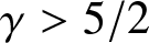 $\gamma \gt 5/2$. Finally, using (2.33) and (2.34), we derive the corresponding lower bounds to (2.30)
 \begin{equation}
Q(K) \geq {\liminf_{L \to \infty}} \mathcal{Q}(W_L) \geq \sum_{m=1}^\infty \Phi_m^{\prime\prime}(\nu m) K m^2,
\end{equation}
\begin{equation}
Q(K) \geq {\liminf_{L \to \infty}} \mathcal{Q}(W_L) \geq \sum_{m=1}^\infty \Phi_m^{\prime\prime}(\nu m) K m^2,
\end{equation}which completes the proof.
Lemma 12. For all  $K$ such that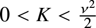 $0 \lt K \lt \frac{\nu^2}{2}$, $P(K) \gt Q(K)$ holds.
Proof. As in the proof of Lemma 11, we consider the family of test functions  $W_L$ defined in (2.31) with parameter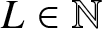 $L \in \mathbb{N}$.
Estimate for  $\mathcal{P}(W_L) - \mathcal{Q}(W_L)$: First we observe that the Taylor expansion
 \begin{equation}
\Phi_m(\nu m - r) = \Phi_m(\nu m) - \Phi_m'( \nu m)r + \Phi_m^{\prime\prime}(\nu m)\frac{r^2}{2} - \Phi_m^{\prime\prime\prime}(\nu m - \theta r)\frac{r^3}{3!}
\end{equation}
\begin{equation}
\Phi_m(\nu m - r) = \Phi_m(\nu m) - \Phi_m'( \nu m)r + \Phi_m^{\prime\prime}(\nu m)\frac{r^2}{2} - \Phi_m^{\prime\prime\prime}(\nu m - \theta r)\frac{r^3}{3!}
\end{equation}with some 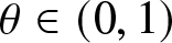 $\theta \in {(0,1)}$ implies
 \begin{equation}
\Psi_m(A_mW(s)) - \Phi_m^{\prime\prime}(\nu m) \frac{(A_mW(s))^2}{2} = -\Phi_m^{\prime\prime\prime}(\nu m - \theta A_m W(s) ) \frac{(A_m W(s))^3}{3!}.
\end{equation}
\begin{equation}
\Psi_m(A_mW(s)) - \Phi_m^{\prime\prime}(\nu m) \frac{(A_mW(s))^2}{2} = -\Phi_m^{\prime\prime\prime}(\nu m - \theta A_m W(s) ) \frac{(A_m W(s))^3}{3!}.
\end{equation} Using Lemma 6 and the fact that  $\Phi_m^{\prime\prime\prime}$ is nonpositive and monotonically increasing, we obtain
 \begin{equation}
-\Phi_m^{\prime\prime\prime}(\nu m - \theta A_m W(s) ) \frac{(A_m W(s))^3}{3!} \geq C_m (A_m W(s))^3
\end{equation}
\begin{equation}
-\Phi_m^{\prime\prime\prime}(\nu m - \theta A_m W(s) ) \frac{(A_m W(s))^3}{3!} \geq C_m (A_m W(s))^3
\end{equation}with the constant  $C_m := -\Phi_m^{\prime\prime\prime}(\nu m)/3! \geq 0$.
Combining (2.32), (2.37) and (2.38), we then obtain
 \begin{align}
\mathcal{P}(W_L) - \mathcal{Q}(W_L) &= \int\limits_{\mathbb{R}} \sum_{m=1}^\infty \Psi_m(A_m W_L(s)) - \Phi_m^{\prime\prime}(\nu m) (A_m W_L(s) )^2 \, {\rm d}s \nonumber\\
&\geq \int\limits_{\mathbb{R}} \sum_{m=1}^\infty C_m (A_m W_L(s))^3
\geq C_1 \int\limits_{-(L-\frac12)}^{L-\frac12} (A_1 W_L(s))^3 \, {\rm d}s \nonumber \\
&= \frac{C_1 K^{\frac32}}{L^\frac32} (2L-1 )
= c_1 (2L^{-\frac12} - L^{-\frac32})
\end{align}
\begin{align}
\mathcal{P}(W_L) - \mathcal{Q}(W_L) &= \int\limits_{\mathbb{R}} \sum_{m=1}^\infty \Psi_m(A_m W_L(s)) - \Phi_m^{\prime\prime}(\nu m) (A_m W_L(s) )^2 \, {\rm d}s \nonumber\\
&\geq \int\limits_{\mathbb{R}} \sum_{m=1}^\infty C_m (A_m W_L(s))^3
\geq C_1 \int\limits_{-(L-\frac12)}^{L-\frac12} (A_1 W_L(s))^3 \, {\rm d}s \nonumber \\
&= \frac{C_1 K^{\frac32}}{L^\frac32} (2L-1 )
= c_1 (2L^{-\frac12} - L^{-\frac32})
\end{align}for the constant  $c_1 := C_1K^{\frac32} \gt 0$. Here, we use the strict negativity of $\Phi^{\prime\prime\prime}_1$ in (1.9).
Estimate for  $Q(K) - \mathcal{Q}(W_L)$: With (2.33) we observe
 \begin{align}
Q(K) - \mathcal{Q}(W_L) &\leq \sum_{m=1}^\infty \Phi_m^{\prime\prime}(\nu m) K m^2 - \sum\limits_{m=1}^{L} \Phi_m^{\prime\prime}(\nu m) K m^2 \Big( 1- \frac{m}{2L} \Big) \nonumber\\
&= \sum\limits_{m=L+1}^{\infty} \Phi_m^{\prime\prime}(\nu m) K m^2 + \sum\limits_{m=1}^{L} \Phi_m^{\prime\prime}(\nu m) K \frac{m^3}{2L}.\end{align}
\begin{align}
Q(K) - \mathcal{Q}(W_L) &\leq \sum_{m=1}^\infty \Phi_m^{\prime\prime}(\nu m) K m^2 - \sum\limits_{m=1}^{L} \Phi_m^{\prime\prime}(\nu m) K m^2 \Big( 1- \frac{m}{2L} \Big) \nonumber\\
&= \sum\limits_{m=L+1}^{\infty} \Phi_m^{\prime\prime}(\nu m) K m^2 + \sum\limits_{m=1}^{L} \Phi_m^{\prime\prime}(\nu m) K \frac{m^3}{2L}.\end{align}Using the global bound in (1.10c), we get for the first sum of (2.40) that
 \begin{equation}
\begin{aligned}
&\sum_{m=L+1}^{\infty} \Phi_m^{\prime\prime}(\nu m) K m^2= K \sum_{m=L+1}^{\infty}
\Phi_m^{\prime\prime}(\nu m) m^\gamma m^{2-\gamma} \\
&\quad \leq K \sum_{m=L+1}^{\infty}
\Phi_m^{\prime\prime}(\nu m) m^\gamma (L+1)^{2-\gamma}= (L+1)^{-(\gamma-2)} K \sum_{m=L+1}^{\infty}\Phi_m^{\prime\prime}(\nu m) m^\gamma \\
&\quad\leq c_2 L^{-(\gamma-2)}.
\end{aligned}
\end{equation}
\begin{equation}
\begin{aligned}
&\sum_{m=L+1}^{\infty} \Phi_m^{\prime\prime}(\nu m) K m^2= K \sum_{m=L+1}^{\infty}
\Phi_m^{\prime\prime}(\nu m) m^\gamma m^{2-\gamma} \\
&\quad \leq K \sum_{m=L+1}^{\infty}
\Phi_m^{\prime\prime}(\nu m) m^\gamma (L+1)^{2-\gamma}= (L+1)^{-(\gamma-2)} K \sum_{m=L+1}^{\infty}\Phi_m^{\prime\prime}(\nu m) m^\gamma \\
&\quad\leq c_2 L^{-(\gamma-2)}.
\end{aligned}
\end{equation}holds with 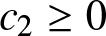 $c_2 \geq 0$.
Analogously, the second sum in (2.40) can be estimated by
 \begin{equation}
\sum\limits_{m=1}^{L} \Phi_m^{\prime\prime}(\nu m) K \frac{m^3}{2L} \leq c_3 \frac{L^{3-\gamma}}{L} = c_3 L^{-(\gamma -2)}, \quad c_3 \geq 0.
\end{equation}
\begin{equation}
\sum\limits_{m=1}^{L} \Phi_m^{\prime\prime}(\nu m) K \frac{m^3}{2L} \leq c_3 \frac{L^{3-\gamma}}{L} = c_3 L^{-(\gamma -2)}, \quad c_3 \geq 0.
\end{equation}Combining all results: We now have
 \begin{align}P(K) \geq \mathcal{P}(W_L) &= \mathcal{Q}(W_L) + \mathcal{P}(W_L) - \mathcal{Q}(W_L) \nonumber \\
&\geq Q(K) - c_2 L^{{-(\gamma -2)}} - c_3 L^{{-(\gamma -2)}} + c_1(2L^{-\frac12} - L^{-\frac32} ) .\end{align}
\begin{align}P(K) \geq \mathcal{P}(W_L) &= \mathcal{Q}(W_L) + \mathcal{P}(W_L) - \mathcal{Q}(W_L) \nonumber \\
&\geq Q(K) - c_2 L^{{-(\gamma -2)}} - c_3 L^{{-(\gamma -2)}} + c_1(2L^{-\frac12} - L^{-\frac32} ) .\end{align} As 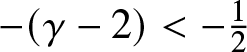 $-(\gamma -2) \lt -\frac12$ by assumption, we obtain the inequality $P(K) \gt Q(K)$ by choosing $L$ finite but sufficiently large.
We are now in the position to prove the main technical step.
Proposition 13. Any sequence  $(W_n)_{n\in\mathbb{N}} \subseteq \mathcal{C}_K$ that satisfies $\lim\limits_{n\to\infty} \mathcal{P}(W_n) = P(K)$ admits a strongly convergent subsequence in $\mathsf{L}^2(\mathbb{R})$.
Proof. Preliminaries: Since  $(W_n)_n$ is a bounded sequence in $\mathsf{L}^2$, there exists a (not relabeled) subsequence with
 \begin{equation}W_n\rightharpoonup W_\infty\quad\text{for}\ n\rightarrow\infty\;\text{weakly in}\,L^2(\mathbb{R}).\end{equation}
 Note that  $\mathcal{C}$ is convex and closed and thus, $W_{\infty} \in \mathcal{C}$. It is our goal to show
 \begin{equation}
\|W_{\infty}\|_2^2 \geq 2K,
\end{equation}
\begin{equation}
\|W_{\infty}\|_2^2 \geq 2K,
\end{equation}since this implies  $\|W_{\infty}\|_2^2 = 2K$ due to
 \begin{equation}
\|W_{\infty}\|_2^2 \leq \liminf\limits_{n\to\infty} \|W_n\|_2^2 = 2K.
\end{equation}
\begin{equation}
\|W_{\infty}\|_2^2 \leq \liminf\limits_{n\to\infty} \|W_n\|_2^2 = 2K.
\end{equation}The strong convergence then follows directly from the weak convergence.
Defining new quantities: For given cut-off parameters  $L,M \in \mathbb{N}$, we define the functions
 \begin{equation}
\widetilde{W}_n(s) := W_n(s) \chi_{[-L,L]}(s) \qquad \text{and} \qquad \overline{W}_n(s) := W_n(s) - \widetilde{W}_n(s)
\end{equation}
\begin{equation}
\widetilde{W}_n(s) := W_n(s) \chi_{[-L,L]}(s) \qquad \text{and} \qquad \overline{W}_n(s) := W_n(s) - \widetilde{W}_n(s)
\end{equation}and the modified quantities
 \begin{equation}
{\mathcal{P}_M}(W) := \sum\limits_{m=1}^{M} \int\limits_{\mathbb{R}} \Psi_m(A_m W(s)) \,{\rm d}s,
\end{equation}
\begin{equation}
{\mathcal{P}_M}(W) := \sum\limits_{m=1}^{M} \int\limits_{\mathbb{R}} \Psi_m(A_m W(s)) \,{\rm d}s,
\end{equation} \begin{equation}
{\mathcal{Q}_M}(W) := \sum\limits_{m=1}^{M} \int\limits_{\mathbb{R}} \frac12 \Phi_m^{\prime\prime}(\nu m) (A_m W(s))^2 \,{\rm d}s.
\end{equation}
\begin{equation}
{\mathcal{Q}_M}(W) := \sum\limits_{m=1}^{M} \int\limits_{\mathbb{R}} \frac12 \Phi_m^{\prime\prime}(\nu m) (A_m W(s))^2 \,{\rm d}s.
\end{equation}We note that the identity
 \begin{equation}
\|\widetilde{W}_n\|_2^2 + \|\overline{W}_n\|_2^2 = \|W_n\|_2^2 = 2K
\end{equation}
\begin{equation}
\|\widetilde{W}_n\|_2^2 + \|\overline{W}_n\|_2^2 = \|W_n\|_2^2 = 2K
\end{equation}holds for all  $n \in \mathbb{N}$.
Approximations: Let  $ \epsilon \gt 0$ be given. Our first observation is that by choosing $M$ large enough (and fixed for use later), we can guarantee
 \begin{equation}
0 \leq | \mathcal{P}(W_n) - {{\mathcal{P}_M}}(W_n)| \leq \sum_{m=M+1}^\infty K m^2 \Phi_m^{\prime\prime}(\nu m - \sqrt{2Km}) \leq \epsilon
\end{equation}
\begin{equation}
0 \leq | \mathcal{P}(W_n) - {{\mathcal{P}_M}}(W_n)| \leq \sum_{m=M+1}^\infty K m^2 \Phi_m^{\prime\prime}(\nu m - \sqrt{2Km}) \leq \epsilon
\end{equation}uniformly in  $\mathcal{C}_K$ due to the estimates in the proof of Lemma 7. Second, for every $m \leq M$, the convolution of $A_m$ with $\widetilde{W}_n$ resp. $\overline{W}_n$ gives for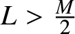 $L \gt \frac{M}{2}$
 \begin{align}
&A_m \widetilde{W}_n(s) = A_m W(s), && \text{if } |s| \leq L-\frac{m}{2}, \nonumber \\
&0 \leq A_m \widetilde{W}_n(s) \leq A_m W_n(s), && \text{if } L-\frac{m}{2} \leq |s| \leq L+\frac{m}{2}, \nonumber \\
&A_m \widetilde{W}_n(s) = 0, && \text{if } |s| \gt L+\frac{m}{2}
\end{align}
\begin{align}
&A_m \widetilde{W}_n(s) = A_m W(s), && \text{if } |s| \leq L-\frac{m}{2}, \nonumber \\
&0 \leq A_m \widetilde{W}_n(s) \leq A_m W_n(s), && \text{if } L-\frac{m}{2} \leq |s| \leq L+\frac{m}{2}, \nonumber \\
&A_m \widetilde{W}_n(s) = 0, && \text{if } |s| \gt L+\frac{m}{2}
\end{align}resp.
 \begin{align}
&A_m \overline{W}_n(s) = 0, && \text{if } |s| \leq L-\frac{m}{2}, \nonumber \\
&0 \leq A_m \overline{W}_n(s) \leq A_m W(s), && \text{if } L-\frac{m}{2} \leq |s| \leq L+\frac{m}{2}, \nonumber \\
&A_m \overline{W}_n(s) = A_m W_n(s), && \text{if } |s| \gt L+\frac{m}{2}.
\end{align}
\begin{align}
&A_m \overline{W}_n(s) = 0, && \text{if } |s| \leq L-\frac{m}{2}, \nonumber \\
&0 \leq A_m \overline{W}_n(s) \leq A_m W(s), && \text{if } L-\frac{m}{2} \leq |s| \leq L+\frac{m}{2}, \nonumber \\
&A_m \overline{W}_n(s) = A_m W_n(s), && \text{if } |s| \gt L+\frac{m}{2}.
\end{align} With that and the monotinicity of  $\Psi_m$, we derive
 \begin{align}
&| {\mathcal{P}_M}(W_n) - {\mathcal{P}_M}(\widetilde{W}_n)- {\mathcal{P}_M}(\overline{W}_n)| \nonumber\\
&= \Big| \sum_{m=1}^M \int\limits_{\mathbb{R}} \Psi_m(A_m W_n(s)) - \Psi_m(A_m \widetilde{W}_n(s)) - \Psi_m(A_m \overline{W}_n(s)) \, {\rm d}s \Big| \nonumber \\
&\leq 2 \sum_{m=1}^M \int\limits_{L-\frac{m}{2}}^{L+\frac{m}{2}} \Psi_m(A_m W_n(s)) \, {\rm d}s \leq 2 \sum_{m=1}^M \int\limits_{L-\frac{M}{2}}^{L+\frac{M}{2}} \Psi_m(A_m W_n(s)) \, {\rm d}s.
\end{align}
\begin{align}
&| {\mathcal{P}_M}(W_n) - {\mathcal{P}_M}(\widetilde{W}_n)- {\mathcal{P}_M}(\overline{W}_n)| \nonumber\\
&= \Big| \sum_{m=1}^M \int\limits_{\mathbb{R}} \Psi_m(A_m W_n(s)) - \Psi_m(A_m \widetilde{W}_n(s)) - \Psi_m(A_m \overline{W}_n(s)) \, {\rm d}s \Big| \nonumber \\
&\leq 2 \sum_{m=1}^M \int\limits_{L-\frac{m}{2}}^{L+\frac{m}{2}} \Psi_m(A_m W_n(s)) \, {\rm d}s \leq 2 \sum_{m=1}^M \int\limits_{L-\frac{M}{2}}^{L+\frac{M}{2}} \Psi_m(A_m W_n(s)) \, {\rm d}s.
\end{align} Furthermore, we note that by the unimodality of 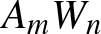 $A_m W_n$
 \begin{align}
\|A_m W_n \|_2^2 &= \int\limits_{\mathbb{R}} \big(A_m W_n (\sigma) \big)^2 \, {\rm d}\sigma \geq \int_{-|s|}^{|s|} \big(A_m W_n (\sigma) \big)^2 \, {\rm d}\sigma \nonumber \\
&\geq \int_{-|s|}^{|s|} \big(A_m W_n (s) \big)^2 \, {\rm d}\sigma = 2|s| \big(A_m W_n(s) \big)^2\end{align}
\begin{align}
\|A_m W_n \|_2^2 &= \int\limits_{\mathbb{R}} \big(A_m W_n (\sigma) \big)^2 \, {\rm d}\sigma \geq \int_{-|s|}^{|s|} \big(A_m W_n (\sigma) \big)^2 \, {\rm d}\sigma \nonumber \\
&\geq \int_{-|s|}^{|s|} \big(A_m W_n (s) \big)^2 \, {\rm d}\sigma = 2|s| \big(A_m W_n(s) \big)^2\end{align}holds for all  $s \in \mathbb{R}$. Hence, we have with Young’s convolution inequality
 \begin{equation}
0 \leq \big(A_m W_n(s)\big)^2 \leq \frac{\|A_m W_n\|_2^2}{2|s|} \leq \frac{\|A_m\|_1^2 \|W_n\|_2^2}{2|s|} = \frac{Km^2}{|s|}.
\end{equation}
\begin{equation}
0 \leq \big(A_m W_n(s)\big)^2 \leq \frac{\|A_m W_n\|_2^2}{2|s|} \leq \frac{\|A_m\|_1^2 \|W_n\|_2^2}{2|s|} = \frac{Km^2}{|s|}.
\end{equation}Using (2.13), (2.54) and (2.56), we find
 \begin{align}| {{\mathcal{P}_M}}(W_n)& - {{\mathcal{P}_M}}(\widetilde{W}_n)- {\mathcal{P}_M}(\overline{W}_n)| \leq 2 \sum_{m=1}^M \int\limits_{L-\frac{M}{2}}^{L+\frac{M}{2}} \frac{\Phi_m^{\prime\prime}(\nu m - \sqrt{2Km})}{2} \big(A_m W_n(s) \big)^2 \, {\rm d}s \nonumber \\
&\leq \sum_{m=1}^M \Phi_m^{\prime\prime}(\nu m - \sqrt{2Km})m^2K \int\limits_{L-\frac{M}{2}}^{L+\frac{M}{2}} \frac{1}{s} \, {\rm d}s = C \ln\Big(\frac{L+\frac{M}{2}}{L-\frac{M}{2}}\Big) \leq \epsilon\end{align}
\begin{align}| {{\mathcal{P}_M}}(W_n)& - {{\mathcal{P}_M}}(\widetilde{W}_n)- {\mathcal{P}_M}(\overline{W}_n)| \leq 2 \sum_{m=1}^M \int\limits_{L-\frac{M}{2}}^{L+\frac{M}{2}} \frac{\Phi_m^{\prime\prime}(\nu m - \sqrt{2Km})}{2} \big(A_m W_n(s) \big)^2 \, {\rm d}s \nonumber \\
&\leq \sum_{m=1}^M \Phi_m^{\prime\prime}(\nu m - \sqrt{2Km})m^2K \int\limits_{L-\frac{M}{2}}^{L+\frac{M}{2}} \frac{1}{s} \, {\rm d}s = C \ln\Big(\frac{L+\frac{M}{2}}{L-\frac{M}{2}}\Big) \leq \epsilon\end{align}for  $L$ large enough and the fixed $M$.
$M$.
With (2.37), Lemma 6 and 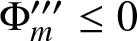 $\Phi^{\prime\prime\prime}_m \leq 0$ respective $\Phi_m^{(4)} \geq 0$ we obtain
 \begin{equation}
{\Psi_m(A_m W(s)) - \frac{\Phi_m^{\prime\prime}(\nu m)}{2}(A_m W(s))^2 \leq - \frac{\Phi_m^{\prime\prime\prime}(\nu m - \sqrt{2Km})}{3!}(A_m W(s))^3.}
\end{equation}
\begin{equation}
{\Psi_m(A_m W(s)) - \frac{\Phi_m^{\prime\prime}(\nu m)}{2}(A_m W(s))^2 \leq - \frac{\Phi_m^{\prime\prime\prime}(\nu m - \sqrt{2Km})}{3!}(A_m W(s))^3.}
\end{equation}With (2.56) and (2.58), we then estimate
 \begin{align}
| {\mathcal{P}_M}(\overline{W}_n) - {\mathcal{Q}_M}(\overline{W}_n) | &=\Big| \sum_{m=1}^M \int\limits_{\mathbb{R}} \Psi_m(A_m\overline{W}_n(s) ) - \frac{\Phi_m^{\prime\prime}(\nu m)}{2} (A_m \overline{W}_n(s))^2 \, {\rm d} s \Big| \nonumber \\
&\leq\Big| \sum_{m=1}^M \int\limits_{\mathbb{R}} -\frac{\Phi_m^{\prime\prime\prime}(\nu m - \sqrt{2Km} )}{3!} (A_m\overline{W}_n(s))^3 \, {\rm d} s \Big| \nonumber \\ & {\leq 2} \Big| \sum_{m=1}^M \int\limits_{L-\frac{m}{2}}^{\infty} \frac{\Phi_m^{\prime\prime\prime}(\nu m - \sqrt{2Km})}{3!} (A_m W_n(s))^3 \, {\rm d} s \Big| \nonumber \\
&\leq 2 \Big| \sum_{m=1}^M \frac{\Phi_m^{\prime\prime\prime}(\nu m - \sqrt{2Km})}{3!} ( {Km^2})^{\frac32} \int\limits_{L-\frac{m}{2}}^{\infty} \frac{1}{s^{\frac32}} \, {\rm d} s \Big|
{\,\leq \epsilon}\end{align}
\begin{align}
| {\mathcal{P}_M}(\overline{W}_n) - {\mathcal{Q}_M}(\overline{W}_n) | &=\Big| \sum_{m=1}^M \int\limits_{\mathbb{R}} \Psi_m(A_m\overline{W}_n(s) ) - \frac{\Phi_m^{\prime\prime}(\nu m)}{2} (A_m \overline{W}_n(s))^2 \, {\rm d} s \Big| \nonumber \\
&\leq\Big| \sum_{m=1}^M \int\limits_{\mathbb{R}} -\frac{\Phi_m^{\prime\prime\prime}(\nu m - \sqrt{2Km} )}{3!} (A_m\overline{W}_n(s))^3 \, {\rm d} s \Big| \nonumber \\ & {\leq 2} \Big| \sum_{m=1}^M \int\limits_{L-\frac{m}{2}}^{\infty} \frac{\Phi_m^{\prime\prime\prime}(\nu m - \sqrt{2Km})}{3!} (A_m W_n(s))^3 \, {\rm d} s \Big| \nonumber \\
&\leq 2 \Big| \sum_{m=1}^M \frac{\Phi_m^{\prime\prime\prime}(\nu m - \sqrt{2Km})}{3!} ( {Km^2})^{\frac32} \int\limits_{L-\frac{m}{2}}^{\infty} \frac{1}{s^{\frac32}} \, {\rm d} s \Big|
{\,\leq \epsilon}\end{align}uniformly in  $n$ by choosing $L$ sufficiently large, using the facts that $A_m\overline{W}_n$ is even and supported in $\mathbb{R} \setminus[-L+\frac{m}{2}, L-\frac{m}{2}]$ and that $M$ is fixed.
In summary, we obtain the estimate, uniformly in  $n$,
$n$,
 \begin{align}
&| \mathcal{P}(W_n) - {\mathcal{P}_M}(\widetilde{W}_n) - {\mathcal{Q}_M}(\overline{W}_n) | \nonumber\\
&\leq |\mathcal{P}(W_n) - {\mathcal{P}_M}(W_n) | + | {\mathcal{P}_M}(W_n) - {\mathcal{P}_M}(\widetilde{W}_n) - {\mathcal{P}_M}(\overline{W}_n) | + | {\mathcal{P}_M}(\overline{W}_n) - {\mathcal{Q}_M}(\overline{W}_n) | \leq 3 \epsilon.\end{align}
\begin{align}
&| \mathcal{P}(W_n) - {\mathcal{P}_M}(\widetilde{W}_n) - {\mathcal{Q}_M}(\overline{W}_n) | \nonumber\\
&\leq |\mathcal{P}(W_n) - {\mathcal{P}_M}(W_n) | + | {\mathcal{P}_M}(W_n) - {\mathcal{P}_M}(\widetilde{W}_n) - {\mathcal{P}_M}(\overline{W}_n) | + | {\mathcal{P}_M}(\overline{W}_n) - {\mathcal{Q}_M}(\overline{W}_n) | \leq 3 \epsilon.\end{align}In particular, this implies
 \begin{equation}
\mathcal{P}(W_n) \leq {\mathcal{P}_M}(\widetilde{W}_n) + {\mathcal{Q}_M}(\overline{W}_n) + 3\epsilon.
\end{equation}
\begin{equation}
\mathcal{P}(W_n) \leq {\mathcal{P}_M}(\widetilde{W}_n) + {\mathcal{Q}_M}(\overline{W}_n) + 3\epsilon.
\end{equation} Moreover, choosing once again  $L$ large enough, we estimate
 \begin{equation}
| {\mathcal{Q}_M}(\overline{W}_{\infty}) | \leq \epsilon.
\end{equation}
\begin{equation}
| {\mathcal{Q}_M}(\overline{W}_{\infty}) | \leq \epsilon.
\end{equation} From now on, let  $L$ be fixed and sufficiently large to satisfy all the above properties.
The weak convergence (2.44)  $W_n \rightharpoonup W_{\infty}$ implies the pointwise convergence
 \begin{equation}
A_m \widetilde{W}_n \xrightarrow{n\to\infty} A_m \widetilde{W}_{\infty}.
\end{equation}
\begin{equation}
A_m \widetilde{W}_n \xrightarrow{n\to\infty} A_m \widetilde{W}_{\infty}.
\end{equation} 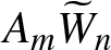 $A_m\widetilde{W}_n$ is supported in $[-L-\frac{m}{2}, L+\frac{m}{2}]$ and bounded by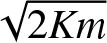 $\sqrt{2Km}$, thus strong convergence
 \begin{equation}
A_m \widetilde{W}_n \xrightarrow{n \to \infty} A_m \widetilde{W}_{\infty}
\end{equation}
\begin{equation}
A_m \widetilde{W}_n \xrightarrow{n \to \infty} A_m \widetilde{W}_{\infty}
\end{equation}follows in  $\mathsf{L}^2$ by Lebesgue’s dominated convergence theorem. With (2.64) we find for sufficiently large $n$
$n$
 \begin{equation}
{\mathcal{P}_M}(\widetilde{W}_n) \leq {\mathcal{P}_M}(\widetilde{W}_{\infty}) + \epsilon.
\end{equation}
\begin{equation}
{\mathcal{P}_M}(\widetilde{W}_n) \leq {\mathcal{P}_M}(\widetilde{W}_{\infty}) + \epsilon.
\end{equation} In addition, since  $(W_n)_{n\in \mathbb{N}}$ is a maximizing sequence, by choosing $n$ sufficiently large, we can ensure
 \begin{equation}
\mathcal{P}(W_n) \geq P(K) - \epsilon.
\end{equation}
\begin{equation}
\mathcal{P}(W_n) \geq P(K) - \epsilon.
\end{equation}With (2.61), (2.65) and (2.66) we then estimate
 \begin{align}
P(K) &\leq \mathcal{P}(W_n) + \epsilon \leq {\mathcal{P}_M}(\widetilde{W}_n) + {\mathcal{Q}_M}(\overline{W}_n) + 4\epsilon \nonumber \\
&\leq {\mathcal{P}_M}(\widetilde{W}_{\infty}) + {\mathcal{Q}_M}(\overline{W}_n) + 5 \epsilon \leq \mathcal{P}(\widetilde{W}_{\infty})+\mathcal{Q}(\overline{W}_n)+5\epsilon.\end{align}
\begin{align}
P(K) &\leq \mathcal{P}(W_n) + \epsilon \leq {\mathcal{P}_M}(\widetilde{W}_n) + {\mathcal{Q}_M}(\overline{W}_n) + 4\epsilon \nonumber \\
&\leq {\mathcal{P}_M}(\widetilde{W}_{\infty}) + {\mathcal{Q}_M}(\overline{W}_n) + 5 \epsilon \leq \mathcal{P}(\widetilde{W}_{\infty})+\mathcal{Q}(\overline{W}_n)+5\epsilon.\end{align} Using  $\|\widetilde{W}_{\infty}\|_2 \leq \|W_{\infty}\|_2 \leq \sqrt{2K}$, see (2.46), and the super-quadraticity of $\mathcal{P}$, we find
 \begin{equation}
\mathcal{P}(\widetilde{W}_{\infty}) \leq \mathcal{P} \Big( \frac{\sqrt{2K}}{\|\widetilde{W}_{\infty}\|_2} \widetilde{W}_{\infty} \Big) \frac{\|\widetilde{W}_{\infty}\|_2^2}{2K} \leq P(K) \frac{\|\widetilde{W}_{\infty}\|_2^2}{2K}.
\end{equation}
\begin{equation}
\mathcal{P}(\widetilde{W}_{\infty}) \leq \mathcal{P} \Big( \frac{\sqrt{2K}}{\|\widetilde{W}_{\infty}\|_2} \widetilde{W}_{\infty} \Big) \frac{\|\widetilde{W}_{\infty}\|_2^2}{2K} \leq P(K) \frac{\|\widetilde{W}_{\infty}\|_2^2}{2K}.
\end{equation}Moreover,
 \begin{equation}
\mathcal{Q}(\lambda W) = \sum_{m=1}^\infty \int\limits_{\mathbb{R}} \frac{\Phi_m^{\prime\prime}(\nu m)}{2} \big( A_m \lambda W (s) \big)^2 = \lambda^2 \mathcal{Q}(W)
\end{equation}
\begin{equation}
\mathcal{Q}(\lambda W) = \sum_{m=1}^\infty \int\limits_{\mathbb{R}} \frac{\Phi_m^{\prime\prime}(\nu m)}{2} \big( A_m \lambda W (s) \big)^2 = \lambda^2 \mathcal{Q}(W)
\end{equation}holds by definition and thus,
 \begin{equation}
\mathcal{Q}(\overline{W}_n) = \mathcal{Q} \Big( \frac{\sqrt{2K}}{\|\overline{W}_n\|_2} \overline{W}_n \Big) \frac{\|\overline{W}_n\|_2^2}{2K} \leq Q(K) \frac{\|\overline{W}_n\|_2^2}{2K}.
\end{equation}
\begin{equation}
\mathcal{Q}(\overline{W}_n) = \mathcal{Q} \Big( \frac{\sqrt{2K}}{\|\overline{W}_n\|_2} \overline{W}_n \Big) \frac{\|\overline{W}_n\|_2^2}{2K} \leq Q(K) \frac{\|\overline{W}_n\|_2^2}{2K}.
\end{equation}With (2.67), (2.68) and (2.70), it follows
 \begin{equation}
P(K) \leq P(K) \frac{\|\widetilde{W}_{\infty}\|_2^2}{2K} + Q(K) \frac{\|\overline{W}_n\|_2^2}{2K} + 5\epsilon.
\end{equation}
\begin{equation}
P(K) \leq P(K) \frac{\|\widetilde{W}_{\infty}\|_2^2}{2K} + Q(K) \frac{\|\overline{W}_n\|_2^2}{2K} + 5\epsilon.
\end{equation} Substituting  $Q(K) = P(K) - (P(K) - Q(K))$ and rearranging the terms in the last inequality implies
 \begin{equation}
P(K) + \frac{\|\overline{W}_n\|_2^2}{2K} (P(K) - Q(K) ) \leq \frac{\|\widetilde{W}_{\infty}\|_2^2 + \|\overline{W}_n\|_2^2}{2K} P(K) + 6\epsilon.
\end{equation}
\begin{equation}
P(K) + \frac{\|\overline{W}_n\|_2^2}{2K} (P(K) - Q(K) ) \leq \frac{\|\widetilde{W}_{\infty}\|_2^2 + \|\overline{W}_n\|_2^2}{2K} P(K) + 6\epsilon.
\end{equation} The weak convergence  $W_n \rightharpoonup W_{\infty}$ implies the weak convergence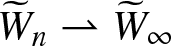 $\widetilde{W}_n \rightharpoonup \widetilde{W}_{\infty}$. This yields
 \begin{equation}
\liminf\limits_{n\to\infty} \|\widetilde{W}_n\|_2 \geq \|\widetilde{W}_{\infty}\|_2
\end{equation}
\begin{equation}
\liminf\limits_{n\to\infty} \|\widetilde{W}_n\|_2 \geq \|\widetilde{W}_{\infty}\|_2
\end{equation}and hence for any  $\epsilon \gt 0$
 \begin{equation}
{\|\widetilde{W}_n\|_2^2 \geq \frac{\|\widetilde{W}_{\infty}\|_2^2}{1+\epsilon}}
\end{equation}
\begin{equation}
{\|\widetilde{W}_n\|_2^2 \geq \frac{\|\widetilde{W}_{\infty}\|_2^2}{1+\epsilon}}
\end{equation}for sufficiently large  $n \in \mathbb{N}$ and $L$ as fixed before. Together with (2.50), it follows
 \begin{equation}
{\|\widetilde{W}_{\infty}\|_2^2+\|\overline{W}_n\|_2^2 \leq (1+\epsilon)\|\widetilde{W}_n\|_2^2 + \|\overline{W}_n\|_2^2 \leq 2K(1+\epsilon)}
\end{equation}
\begin{equation}
{\|\widetilde{W}_{\infty}\|_2^2+\|\overline{W}_n\|_2^2 \leq (1+\epsilon)\|\widetilde{W}_n\|_2^2 + \|\overline{W}_n\|_2^2 \leq 2K(1+\epsilon)}
\end{equation}for  $n$ large enough. Combining the results from (2.72) and (2.75) we find
 \begin{equation}
\|\overline{W}_n\|_2^2 \leq \frac{2K ( P(K) + {6})}{P(K)-Q(K)}\epsilon = C \epsilon.
\end{equation}
\begin{equation}
\|\overline{W}_n\|_2^2 \leq \frac{2K ( P(K) + {6})}{P(K)-Q(K)}\epsilon = C \epsilon.
\end{equation}Inserting this into (2.71), we find the approximation
 \begin{equation}
{P(K) \leq P(K) \frac{\|\widetilde{W}_{\infty}\|_2^2}{2K} + \tilde{C} \epsilon \leq P(K) \frac{\|W_{\infty}\|_2^2}{2K} + \tilde{C} \epsilon }
\end{equation}
\begin{equation}
{P(K) \leq P(K) \frac{\|\widetilde{W}_{\infty}\|_2^2}{2K} + \tilde{C} \epsilon \leq P(K) \frac{\|W_{\infty}\|_2^2}{2K} + \tilde{C} \epsilon }
\end{equation}which implies
 \begin{equation}
{\|W_{\infty}\|_2^2 \geq 2K }
\end{equation}
\begin{equation}
{\|W_{\infty}\|_2^2 \geq 2K }
\end{equation}by choosing  $\epsilon \gt 0$ sufficiently small.
2.3. Proof of main theorem
We are now in the position to complete the proof of our main result.
Proof of Theorem 2
Proposition 11 implies that there exists a maximizer 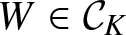 $W \in \mathcal{C}_K$ of $\mathcal{P}$ that can be constructed as the limit point of a maximizing sequence. According to Lemma 10, this maximizer is a solution to (1.6).
We end this section by stating some properties for the wave speed of such solutions.
Lemma 14. Let  $(W_K, c_K)$ be a solution provided by Theorem 2. Then
 \begin{equation}
c_K = \mu(W_K)^{-\frac12} \quad \text{and} \quad
2 c_K^2 \geq \frac{\mathcal{P}(W_K)}{\mathcal{K}(W_K)} = \frac{P(K)}{K}
\end{equation}
\begin{equation}
c_K = \mu(W_K)^{-\frac12} \quad \text{and} \quad
2 c_K^2 \geq \frac{\mathcal{P}(W_K)}{\mathcal{K}(W_K)} = \frac{P(K)}{K}
\end{equation}hold.
Proof. Using that  $W_K$ is a maximizer, the first statement follows directly from Lemma 10. To show the other one, we test the equation
 \begin{equation}
W_K =
\mathcal{T}(W_K) = \mu(W_K)\partial\mathcal{P}(W_K)
\end{equation}
\begin{equation}
W_K =
\mathcal{T}(W_K) = \mu(W_K)\partial\mathcal{P}(W_K)
\end{equation}with  $W_K$. This yields
 \begin{equation}
c_K^2= \frac{1}{\mu(W_K)}= \frac{\langle \partial\mathcal{P}(W_K), W_K \rangle}{\langle W_K, W_K \rangle} \geq
\frac{\mathcal{P}(W_K)}{2\mathcal{K}(W_K)} = \frac{P(K)}{2K}
\end{equation}
\begin{equation}
c_K^2= \frac{1}{\mu(W_K)}= \frac{\langle \partial\mathcal{P}(W_K), W_K \rangle}{\langle W_K, W_K \rangle} \geq
\frac{\mathcal{P}(W_K)}{2\mathcal{K}(W_K)} = \frac{P(K)}{2K}
\end{equation}after evaluating (2.23) with  $V=0$ and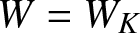 $W=W_K$.
3. High-energy limit
In this section we study the case where the kinetic energy
 \begin{equation}
\mathcal{K}(W) = \frac12 \int\limits_{\mathbb{R}} \big( W(s) \big) ^2 \, {\rm d}s
\end{equation}
\begin{equation}
\mathcal{K}(W) = \frac12 \int\limits_{\mathbb{R}} \big( W(s) \big) ^2 \, {\rm d}s
\end{equation}of the travelling wave profile  $W$ converges to the high-energy limit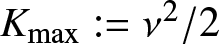 $K_{\text{max}} := \nu^2/2$. A very detailed analysis of these asymptotics for nearest neighbour FPUT is given in [Reference Herrmann and Matthies5]. The high-energy limit is dominated by the nearest neighbour interaction in our setting too; hence, we expect that we could adapt the detailed analysis to the solution constructed in Theorem 2. A simpler analysis can still describe the limit behaviour. For that, we again adapt the ideas of [Reference Herrmann and Matthies7]. Our analysis generalizes results in [Reference Ingimarson and Pego9], where the high-energy limit for the Calogero–Moser lattice is studied, to a general class of interaction potentials.
For simplifications, we restrict our considerations to the special case
 \begin{equation}
\Phi_m(r) = r^{-\alpha}
\end{equation}
\begin{equation}
\Phi_m(r) = r^{-\alpha}
\end{equation}for some fixed  $\alpha \gt \frac32$ and all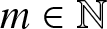 $m \in \mathbb{N}$. Indeed, we only require the specific singularity for $m=1$. The simplification implies
 \begin{equation}
\Psi_m(r) = (\nu m - r)^{-\alpha} - (\nu m)^{-\alpha} - \alpha (\nu m)^{-\alpha-1} r.
\end{equation}
\begin{equation}
\Psi_m(r) = (\nu m - r)^{-\alpha} - (\nu m)^{-\alpha} - \alpha (\nu m)^{-\alpha-1} r.
\end{equation} To start, let  $0 \lt \delta \lt 1$ be a fixed value and consider a maximizing function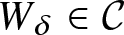 $W_{\delta} \in \mathcal{C}$ with
 \begin{equation}
\mathcal{K}(W_{\delta}) = \big(1-\delta\big) \frac{\nu^2}{2}, \qquad \mathcal{P}(W_{\delta}) = P\Big(\big(1-\delta\big)\frac{\nu^2}{2}\Big).
\end{equation}
\begin{equation}
\mathcal{K}(W_{\delta}) = \big(1-\delta\big) \frac{\nu^2}{2}, \qquad \mathcal{P}(W_{\delta}) = P\Big(\big(1-\delta\big)\frac{\nu^2}{2}\Big).
\end{equation} The first equation in (3.4) ensures that the kinetic energy 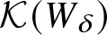 $\mathcal{K}(W_{\delta})$ tends to $K_{\text{max}}$ for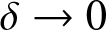 $\delta \to 0$. The second equation means that we choose $W_{\delta}$ to be a maximizer as we proved in the previous section, which might not be unique. It is our goal to analyse the limit $W_{\delta}$ for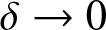 $\delta \to 0$. For this, we define the function
 \begin{equation}
W_0(x) := \nu \chi_{[-1/2, 1/2]}(x) = \begin{cases}
\nu, & x \in [-\frac12, \frac12], \\
0, & x \notin [-\frac12, \frac12].
\end{cases}
\end{equation}
\begin{equation}
W_0(x) := \nu \chi_{[-1/2, 1/2]}(x) = \begin{cases}
\nu, & x \in [-\frac12, \frac12], \\
0, & x \notin [-\frac12, \frac12].
\end{cases}
\end{equation} We will show that  $W_0$ is indeed the correct candidate for the limit of $W_{\delta}$. As a first indication that this could be true, note the following lemma.
Lemma 15. The function  $W_0$ as in (3.5) satisfies $\mathcal{K}(W_0) = K_{\text{max}}$.
Proof. This is a simple direct computation.
Before formulating the convergence result, we also define the auxiliary variables
 \begin{equation}
U_{\delta, m} := A_m W_{\delta} , \qquad \epsilon_{\delta, m} := \nu m - U_{\delta, m}(0)
\end{equation}
\begin{equation}
U_{\delta, m} := A_m W_{\delta} , \qquad \epsilon_{\delta, m} := \nu m - U_{\delta, m}(0)
\end{equation}for all 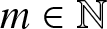 $m \in \mathbb{N}$. The functions $U_{\delta, m}$ are unimodal by construction, and thus the parameters $\epsilon_{\delta, m}$ denote the maximal distances between $U_{\delta, m}$ and the arguments of the singularities of $\Psi_m$, namely $\nu m$.
What follows is the main result of this section.
Theorem 16. We have 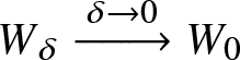 $W_{\delta} \xrightarrow{\delta \to 0} W_0$ strongly in $\mathsf{L}^2(\mathbb{R})$ and $c_{\delta}^2 \xrightarrow{\delta \to 0} \infty$. Here, $c_{\delta}$ denotes the wave speed of $W_{\delta}$.
Proof. Auxiliary results: At first, we note that by Lemma 6
 \begin{equation}
\epsilon_{\delta, m}\geq \nu(m -\sqrt{m}),
\end{equation}
\begin{equation}
\epsilon_{\delta, m}\geq \nu(m -\sqrt{m}),
\end{equation}which is uniformly bounded away from  $0$ for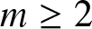 $m\geq 2$.
We want to show the convergence  $\epsilon_{\delta, 1} \xrightarrow{\delta \to 0} 0$. For that, we first notice that
 \begin{equation}
\mathcal{K}\big(\sqrt{1-\delta}\, W_0\big) = \big(1-\delta\big) \frac{\nu^2}{2} = \mathcal{K}(W_{\delta}) =: \mathcal{K}_{\delta}
\end{equation}
\begin{equation}
\mathcal{K}\big(\sqrt{1-\delta}\, W_0\big) = \big(1-\delta\big) \frac{\nu^2}{2} = \mathcal{K}(W_{\delta}) =: \mathcal{K}_{\delta}
\end{equation}holds by construction and
 \begin{equation}
A_1 W_0 (s) = \int\limits_{-\frac12}^{\frac12} \nu \, \chi_{[-1/2, 1/2]} (s + \sigma) \, {\rm d} \sigma = \begin{cases}
(s+1)\nu, & -1 \leq s \leq 0, \\
(1-s)\nu, & 0 \lt s \leq 1, \\
0, & s \notin [-1, 1]
\end{cases}
\end{equation}
\begin{equation}
A_1 W_0 (s) = \int\limits_{-\frac12}^{\frac12} \nu \, \chi_{[-1/2, 1/2]} (s + \sigma) \, {\rm d} \sigma = \begin{cases}
(s+1)\nu, & -1 \leq s \leq 0, \\
(1-s)\nu, & 0 \lt s \leq 1, \\
0, & s \notin [-1, 1]
\end{cases}
\end{equation}is a tent-shaped function with support in 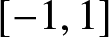 $[-1, 1]$.
Using that  $W_{\delta}$ is a maximizer of the potential energy among all functions with a kinetic energy of $K_{\delta}$, along with (3.8) and (3.9) and the continuity of $\Psi_1$, it follows
 \begin{align}
\mathcal{P}&(W_{\delta}) \geq \mathcal{P}(\sqrt{1-\delta}\, W_0) \geq \int\limits_{\mathbb{R}} \Psi_1(A_1 \sqrt{1-\delta} W_0(s) ) \, {\rm d}s \nonumber \\
&\xrightarrow{\delta \to 0} \int\limits_{\mathbb{R}} \Psi_1(A_1 W_0(s) ) \, {\rm d}s = 2 \int_0^1 \Psi_1 ( (1-s) \nu ) \, {\rm d}s = \infty\end{align}
\begin{align}
\mathcal{P}&(W_{\delta}) \geq \mathcal{P}(\sqrt{1-\delta}\, W_0) \geq \int\limits_{\mathbb{R}} \Psi_1(A_1 \sqrt{1-\delta} W_0(s) ) \, {\rm d}s \nonumber \\
&\xrightarrow{\delta \to 0} \int\limits_{\mathbb{R}} \Psi_1(A_1 W_0(s) ) \, {\rm d}s = 2 \int_0^1 \Psi_1 ( (1-s) \nu ) \, {\rm d}s = \infty\end{align}by a direct computation. Suppose for the moment that  $\epsilon_{\delta, 1}$ does not converge to zero. Then there exists a constant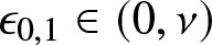 $\epsilon_{0,1} \in (0,\nu)$ such that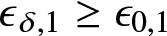 $\epsilon_{\delta, 1} \geq \epsilon_{0,1}$ applies to a fixed sequence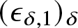 $(\epsilon_{\delta, 1})_{\delta}$ for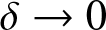 $\delta \to 0$. With the definition and unimodality of $U_{\delta, 1}$ and the definition of $\epsilon_{\delta, 1}$, it follows that
 \begin{equation}
\| A_1 W_{\delta}\|_{\infty} = A_1 W_{\delta}(0) = U_{\delta, 1}(0) = \nu - \epsilon_{\delta,1} \leq \nu - \epsilon_{0,1}
\end{equation}
\begin{equation}
\| A_1 W_{\delta}\|_{\infty} = A_1 W_{\delta}(0) = U_{\delta, 1}(0) = \nu - \epsilon_{\delta,1} \leq \nu - \epsilon_{0,1}
\end{equation}holds. This implies a strictly positive distance between 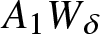 $A_1 W_{\delta}$ and the argument $\nu$ of the singularity of $\Psi_1$ for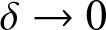 $\delta \to 0$. Due to (3.7), this distance result between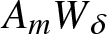 $A_m W_{\delta}$ and its corresponding singularity $\nu m$ holds for all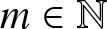 $m \in \mathbb{N}$. With the arguments in the proof of Lemma 7, it follows that the limit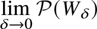 $\lim\limits_{\delta \to 0} \mathcal{P}(W_{\delta})$ is finite. This is a contradiction to (3.10), and therefore we conclude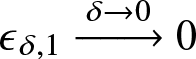 $\epsilon_{\delta, 1} \xrightarrow{\delta \to 0} 0$.
Proof of the statement: With
 \begin{equation}
U_{\delta, 1}(0) = (A_1 W_{\delta})(0) = \int\limits_{-\frac{1}{2}}^{\frac{1}{2}} W_{\delta}(x) \, {\rm d}x
= \int\limits_{\mathbb{R}} \chi_{[-1/2, 1/2]}(x) W_{\delta}(x) \, {\rm d}x = \langle W_{\delta}, \chi_{[-1/2, 1/2]} \rangle
\end{equation}
\begin{equation}
U_{\delta, 1}(0) = (A_1 W_{\delta})(0) = \int\limits_{-\frac{1}{2}}^{\frac{1}{2}} W_{\delta}(x) \, {\rm d}x
= \int\limits_{\mathbb{R}} \chi_{[-1/2, 1/2]}(x) W_{\delta}(x) \, {\rm d}x = \langle W_{\delta}, \chi_{[-1/2, 1/2]} \rangle
\end{equation}we observe
 \begin{equation}
\langle W_{\delta}, W_0 \rangle = \nu \langle W_{\delta}, \chi_{[-1/2, 1/2]} \rangle = \nu U_{\delta, 1}(0).
\end{equation}
\begin{equation}
\langle W_{\delta}, W_0 \rangle = \nu \langle W_{\delta}, \chi_{[-1/2, 1/2]} \rangle = \nu U_{\delta, 1}(0).
\end{equation} With 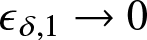 $\epsilon_{\delta,1} \to 0$, it follows
 \begin{align}\|W_{\delta} - W_0 \|_2^2 &= \|W_{\delta}\|_2^2 + \|W_0\|_2^2 - 2 \langle W_{\delta}, W_0 \rangle = 2 \mathcal{K}_{\delta} + 2 K_{\text{max}} - 2 \nu U_{\delta, 1}(0) \nonumber \\
&= (1-\delta)\nu^2 + \nu^2 - 2 \nu^2 + 2\epsilon_{\delta,1} \nu = 2\epsilon_{\delta,1}\nu - \delta \nu^2 \xrightarrow{\delta \to 0} 0.\end{align}
\begin{align}\|W_{\delta} - W_0 \|_2^2 &= \|W_{\delta}\|_2^2 + \|W_0\|_2^2 - 2 \langle W_{\delta}, W_0 \rangle = 2 \mathcal{K}_{\delta} + 2 K_{\text{max}} - 2 \nu U_{\delta, 1}(0) \nonumber \\
&= (1-\delta)\nu^2 + \nu^2 - 2 \nu^2 + 2\epsilon_{\delta,1} \nu = 2\epsilon_{\delta,1}\nu - \delta \nu^2 \xrightarrow{\delta \to 0} 0.\end{align}Finally, the statement
 \begin{equation}
c^2_{\delta} \geq \frac{\mathcal{P}(W_{\delta})}{2 \mathcal{K}(W_{\delta})} \xrightarrow{\delta \to 0} \infty
\end{equation}
\begin{equation}
c^2_{\delta} \geq \frac{\mathcal{P}(W_{\delta})}{2 \mathcal{K}(W_{\delta})} \xrightarrow{\delta \to 0} \infty
\end{equation}is a direct consequence of Lemma 14 and the divergence of  $\mathcal{P}(W_{\delta})$.
Acknowledgements
The work presented in this paper began in spring 2024. We had already made some good progress at the time of the unexpected death of the first author on July 21, 2024. We would like to dedicate this paper to the memory of our good friend Michael Herrmann.
The authors are very grateful for the helpful comments by the referees.
Funding statement
This work was partially supported by the EPSRC Centre for Doctoral Training in Statistical Applied Mathematics at Bath (SAMBa) under grant number EP/S022945/1.

 Open access

