The HW distribution, usually called Hardy–Weinberg equilibrium (HWE),

(1) \begin{equation} \{ q^2 ,2q(1 - q),(1 - q)^2 \} ,\end{equation}

is widely used in population genetics as a base or platform for development of theory and analysis (Edwards, Reference Edwards2008; Hartl & Jones, Reference Hartl and Jones2006; Mayo, Reference Mayo2008; Penrose, Reference Penrose1972; Russell, Reference Russell2006). In (1), q is the frequency (proportion) of one of two alleles in the population. Stark and Seneta (Reference Stark and Seneta2014) have given a more general model, referred to as general mating equilibrium (GME), which does not assume RM. There are many examples in the genetics literature where genotypic proportions close to HW proportions have been observed. When subject to statistical test, they are found to be not significantly different from HW proportions. In other cases, it may be of interest to estimate the degree of divergence from HW proportions, which is measured by an index F, sometimes called the fixation index, at other times the coefficient of inbreeding. The GME model is partly characterized by the marginal distribution of F, which is described below. Here, given a sample of genotypic counts {n_UU , n_UT , n_TT }, I suggest that this distribution is a credible prior distribution of F that can be employed to yield the posterior distribution of F, a procedure called Bayesian, since it uses a formula introduced by Bayes (Reference Bayes1763).

The mating system is defined completely by the matrix C, as described in the next section. Because the specification of the limits of its elements requires some detail, a geometrical description is used. However, this is simply a device to simplify the presentation.

Much of the appeal of the HW model, as published by Hardy (Reference Hardy1908) and Weinberg (Reference Weinberg1908), is due to its apparent simplicity. Weinberg (Reference Weinberg1909), in his review of the first edition of Johannsen's monumental book published in the same year, states that Johannsen erred in attributing the model to Hardy, since Weinberg said it was due to [Karl] Pearson and, following Pearson, to himself. Stern (Reference Stern1943) brought Weinberg's paper to the attention of the genetics community generally. Crow (Reference Crow1999) explains the slowness of recognition of Weinberg's contribution to genetic analysis in the English-speaking world.

Li (Reference Li1988) showed that it is possible to have HWE with non-random mating (NRM), hence Li's phrase ‘pseudo-random mating’. The same possibility is implicit in a formula of Stark (Reference Stark1980). Stark (Reference Stark2006a) showed that it is possible to reach HW form with one round of NRM. It is still possible to find statements that RM is a necessary condition for HW proportions — for example, on page 664 of Russell (Reference Russell2006), though this is by no means rare. Weinberg (Reference Weinberg1908) used the HW distribution to analyze the inheritance of twinning in man. Stark (Reference Stark2006b) noted that Weinberg's analysis may need to be modified in the light of Li's paper. Stark and Seneta (Reference Stark and Seneta2012) show that a paper of a Russian mathematician S. N. Bernstein was a fundamental, though largely unrecognized, contribution to genetic analysis by reason of its connection with the HW law.

The GME model is more general than HWE, since it applies to a range of values of F and so includes HWE (F = 0) as a special case.

Schull (Reference Schull, Neel, Shaw and Schull1965) has a section on the estimation of the coefficient of inbreeding which he defines as:

\begin{equation*} F = \sum {\left( {\left( {\frac{1}{2}} \right)^{n_s + n_d + 1} (1 + F_A )} \right)} , \end{equation*}

where F_A is the coefficient of inbreeding of any common ancestor that makes the connecting link between a line of ancestry tracing back from the sire and one tracing back from the dam. The numbers of generations from sire and dam to such a common ancestor are designated n_s and n_d respectively. Schull says that this concept may be extended to a population average coefficient of inbreeding. This interpretation may be applied to F as used in this paper. Schull describes practical and theoretical difficulties in estimating F, presumably based partly on experiences reported in Schull et al. (Reference Schull, Yanase and Nemoto1962). In particular, Schull gives an example of the instability of some orthodox methods of estimating F. Schull et al. (Reference Schull, Yanase and Nemoto1962) estimated F to be about 0.006 in their study. Neel and Schull (1954, p. 73) give the following formula for the frequency with which recessively inherited conditions arise from consanguineous marriages:

\begin{equation*} Fq + (1 - F)q^2 . \end{equation*}

If the gene frequency of the deleterious gene is q = 1/1,000 and F = 0.006, the condition is about seven times more frequent in the inbred population than in a population in which F = 0.

The need to estimate F arises in forensic investigations. Balding and Nichols (Reference Balding and Nichols1995) give a formula which contains F. In explaining use of the formula, they say that F is analogous to F _ST of Sewall Wright; that is, it concerns stratification of populations in which gene frequencies vary from stratum to stratum. Ayres and Balding (Reference Ayres and Balding1998) use symbol f, ‘a parameter measuring departure from HW caused by inbreeding’. They discuss a number of difficulties associated with estimating f, including choice of prior distributions of f, but do not consider the choice of a logical prior such as that given here. They give a composite posterior distribution of f calculated from a sample of Samoans resident in New Zealand, which has a mode at about f = 0.05.

Cavalli-Sforza and Bodmer (1971, pp. 377–379) have a short section on estimating F, having in mind deviation from HWE due to inbreeding. This method would be classified as orthodox and so is outside the scope of this article.

In the next section, for convenience, I summarize the essential features of GME. The following section gives the marginal distribution of F, then the Bayesian estimation procedure with the aid of an example, and finally a brief discussion mainly about Fisher's (1959) view of the appropriate use of Bayes’ formula.

The General Mating Equilibrium Model

We deal only with a single autosomal locus with two alleles U and T with frequencies in the population q and p (q + p = 1). Throughout, q remains constant because this is guaranteed by the nature of the selected mating system. A set of frequencies of genotypes {UU, UT, TT} can be represented in terms of q and a measure of departure from HW form F as, say, a′ = {q ² + Fpq, 2pq − 2Fpq, p ² + Fpq}. These will vary according to F and will be denoted generally by {f ₀, f _1, f ₂}, (f ₀ + f ₁ + f ₂ = 1), that is f ₀ = q ² + Fpq, and so on.

The population is maintained in discrete generations according to the mating scheme:

(2) \begin{equation} \left[ {\begin{array}{*{20}c} {UU \times UU} &\quad {UU \times UT} &\quad {UU \times TT} \\ {UT \times UU} &\quad {UT \times UT} &\quad {UT \times TT} \\ {TT \times UU} &\quad {TT \times UT} &\quad {TT \times TT} \end{array}} \right]\end{equation}

with commensurate pairing frequencies given by the matrix

(3) \begin{equation} C = \left[ {\begin{array}{*{20}c} {f_{00} } &\quad {f_{01} } &\quad {f_{02} } \\ {f_{10} } &\quad {f_{11} } &\quad {f_{12} } \\ {f_{20} } &\quad {f_{21} } &\quad {f_{22} } \end{array}} \right].\end{equation}

C is symmetric, that is f_ij = f_ji , with row and column sums {f ₀, f ₁, f ₂}. This triple of sums is the parental frequency distribution.

Below we use C in the extended (row vector) form

(4) \begin{equation} u' = \{ f_{00} ,f_{01} ,f_{02} ,f_{10} ,f_{11} ,f_{12} ,f_{20} ,f_{21} ,f_{22} \} .\end{equation}

To follow the progression of generations, we need Mendel's coefficients of heredity given in matrix form by

(5) \begin{eqnarray} M &=& \left[ {\begin{array}{*{20}c} 1 &\quad {{1 \mathord{\left/ {\vphantom {1 2}} \right. \kern-\nulldelimiterspace} 2}} &\quad 0 &\quad {{1 \mathord{\left/ {\vphantom {1 2}} \right. \kern-\nulldelimiterspace} 2}} &\quad {{1 \mathord{\left/ {\vphantom {1 4}} \right. \kern-\nulldelimiterspace} 4}} &\quad 0 &\quad 0 &\quad 0 &\quad 0 \\ 0 &\quad {{1 \mathord{\left/ {\vphantom {1 2}} \right. \kern-\nulldelimiterspace} 2}} &\quad 1 &\quad {{1 \mathord{\left/ {\vphantom {1 2}} \right. \kern-\nulldelimiterspace} 2}} &\quad {{1 \mathord{\left/ {\vphantom {1 2}} \right. \kern-\nulldelimiterspace} 2}} &\quad {{1 \mathord{\left/ {\vphantom {1 2}} \right. \kern-\nulldelimiterspace} 2}} &\quad 1 &\quad {{1 \mathord{\left/ {\vphantom {1 2}} \right. \kern-\nulldelimiterspace} 2}} &\quad 0 \\ 0 &\quad 0 &\quad 0 &\quad 0 &\quad {{1 \mathord{\left/ {\vphantom {1 4}} \right. \kern-\nulldelimiterspace} 4}} &\quad {{1 \mathord{\left/ {\vphantom {1 2}} \right. \kern-\nulldelimiterspace} 2}} &\quad 0 &\quad {{1 \mathord{\left/ {\vphantom {1 2}} \right. \kern-\nulldelimiterspace} 2}} &\quad 1 \end{array}} \right].\nonumber\\&&\end{eqnarray}

Then, the frequency distribution of juveniles is calculated from

\begin{equation*} j' = (Mu)'\end{equation*}

which in detail is

(6) \begin{eqnarray} j &=& \Bigg\{ f_{00} + \frac{f_{01} + f_{10} }{2} + \frac{f_{11} }{4},\frac{f_{01} }{2} + f_{02} \nonumber\\ && + \frac{f_{10} + f_{11} + f_{12} }{2} + f_{20} \nonumber\\ &&+ \frac{f_{21} }{2},\frac{f_{11} }{4} + \frac{f_{12} + f_{21}} {2} + f_{22} \Bigg\}^\prime .\end{eqnarray}

The population is in equilibrium, that is, the distribution of juveniles is the same as that of adults, if and only if matrix C has, in addition to the properties given above, the special property

(7) \begin{equation} f_{11} = 4f_{02} = 4f_{20} .\end{equation}

The notation used here is a modified version of that given in Stark and Seneta (Reference Stark and Seneta2013, Reference Stark and Seneta2014).

By way of explanation, special condition (7), on the system of mate choice, is that the frequency of mating pairs heterozygote × heterozygote is four times the frequency of each of the reciprocal mating pairs homozygote × opposite homozygote. This applies to HWE under RM where the first kind of mating has frequency (2pq)² and each of the second kind (q ²) × (p ²). Under this condition, the ‘loss’ of heterozygotes from the first kind of mating is exactly compensated by the ‘gain’ from the second kind of mating. Identity (7) allows for NRM as well as RM.

Matrix C is a complete description of the mating system. However, the elements of C are subject to various constraints that are conveniently delineated by a geometrical figure that consists of two tetrahedrons, one of which is contained within the other, as shown schematically in Figure 1. For the reader's convenience, the characteristics of this figure are spelled out in more detail below using schematics from Stark and Seneta (Reference Stark and Seneta2014).

FIGURE 1

Schematic illustration of the bounding region of admissible sets of F, f ₁₁, and f ₀₁, for 1/4 < q < 1/2.

Note: The admissible region is defined by the vertices Q, V, Z, D, E, A. The region defined by vertices O, Q, A, and E is not part of the admissible region. The coordinates of the vertices are given in Table 1. Coordinates of points of reference not shown on Table 1 are: O 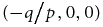${{( - q} \mathord{\left/ {\vphantom {{( - q} p}} \right. \kern-\nulldelimiterspace} p},0,0)$ ; B ((p − 2q)/(3p), 0, 0); N ((2p − q)/(3p), 0, 0).

I assume first that q is fixed so C is defined by the trio (F, f ₁₁, f ₀₁), which can be depicted by points in Euclidean space using orthogonal coordinate axes as shown in Figure 2. The regions of admissible points are of three main types, depending on q: (1) ${1 \mathord{\left/ {\vphantom {1 4}} \right. \kern-\nulldelimiterspace} 4} < q < {1 \mathord{\left/ {\vphantom {1 2}} \right. \kern-\nulldelimiterspace} 2}$ ; (2) $q \le {1 \mathord{\left/ {\vphantom {1 4}} \right. \kern-\nulldelimiterspace} 4}$ ; (3) $q = {1 \mathord{\left/ {\vphantom {1 2}} \right. \kern-\nulldelimiterspace} 2}$ . The faces of the regions are planar, the planes defined by f ₁₁ = 0 (Λ₁) and f ₀₁ = 0 (Λ₂) being two main ones. The remaining planes are defined by the following equations:

\begin{eqnarray*} \Lambda _3 \quad 4pqF - f_{11} - 4f_{01} + 4q^2 = 0\\ \Lambda _4 \quad 2pqF + f_{11} + f_{01} - 2pq = 0\\ \Lambda _5 \quad 12pqF + 3f_{11} + 4f_{01} + 4p(p - 2q) = 0. \end{eqnarray*}

FIGURE 2

Orthogonal axes used to specify coordinates F, f ₁₁, and f ₀₁ for given q.

Only planes Λ₁–Λ₄ are relevant when q < ¼. The respective admissible regions are shown schematically in Figures 5, 3, and 4.

FIGURE 3

Schematic illustration of the bounding region of admissible sets of F, f ₁₁, and f ₀₁ for q ≤ 1/4; vertex O replaces A when q < 1/4.

FIGURE 4

Schematic illustration of the bounding region of admissible sets of F, f ₁₁, and f ₀₁ for q = 1/2.

FIGURE 5

Schematic illustration of the bounding region of admissible sets of F, f ₁₁, and f ₀₁ for 1/4 < q < 1/2.

The Marginal Distribution of F

Case q ⩽ 1/4

This section describes properties of the model depicted in Figure 3 of Stark and Seneta, Reference Stark and Seneta2014 — reproduced here as Figure 3. Suppose that it defines a trivariate distribution of variables F, f ₁₁, and f ₀₁, which maintain a genotypic distribution {f ₀ = q ² + Fpq, f ₁ = 2pq − 2Fpq, f ₂ = p ² + Fpq}. Suppose further that points are distributed uniformly within the space enclosed by the bounding planes. For fixed $q \le {1 \mathord{\left/ {\vphantom {1 4}} \right. \kern-\nulldelimiterspace} 4}$ , the volume enclosed is S = 4q ²/(27p). This can be demonstrated by taking slices of the solid around values of f ₁₁, giving triangles with base (4q − 3f ₁₁)/(4pq), (p = 1 − q), and height (4q − 3f ₁₁)/6. The area of a triangular section is (16q ² − 24qf ₁₁ + 9f ² ₁₁)/(48pq). Integrating this quantity with respect to f ₁₁ over the range 0 to 4q/3, which are the limits of f ₁₁, gives the volume.

Suppose that a population with a particular gene frequency q arrives randomly at some point within the defined space. The value of F will be governed by the marginal distribution of F, here denoted by Π(F). This function has the following values:

(8) \begin{equation} \Pi _1 (F) \ =\ 2f_0^2 /S,\quad - q/p \le F \le (p - 2q)/(3p)\\ \end{equation}

(9) \begin{eqnarray} \Pi _2 (F) &=& 2[q^2 + (f_1 - f_0 )(4f_0 - f_1 )]/(9S),\nonumber\\ && (p - 2q)/(3p) < F \le (2p - q)/(3p)\\ \end{eqnarray}

(10) \begin{equation} \Pi _3 (F) \ =\ f_1^2 /(2S),\quad (2p - q)/(3p) < F \le 1.\end{equation}

The distribution of F, Π(F), has mode (p – q)/(2p). This can be demonstrated by differentiating Π₂(F) with respect to F and equating the derivative to zero. The mode is midway between (p − 2q)/(3p) and (2p − q)/(3p), consistent with the fact that Π(F) is symmetrical about the mode. The distribution at the mode is $f_0 = {q \mathord{\left/ {\vphantom {q 2}} \right. \kern-\nulldelimiterspace} 2}$ , f ₁ = q, $f_2 = {{(2p - q)} \mathord{\left/ {\vphantom {{(2p - q)} 2}} \right. \kern-\nulldelimiterspace} 2}$ .

The symmetry of Π₂(F) can be demonstrated by calculating the value of (f ₁ − f ₀)(4f ₀ − f ₁) at points equidistant from modal F. For a point above the mode, take F ⁺ = (p − q + Δ)/(2p), (Δ > 0), and the corresponding one below F ⁻ = (p − q − Δ)/(2p). Taking first F ⁻, f ₁ − f ₀ = q(1 + 3Δ)/2, and 4f ₀ − f ₁ = q(1 − 3Δ), so (f ₁ − f ₀)(4f ₀ − f ₁) = q ²(1 − 9Δ²)/2. In the case of F ⁺, f ₁ − f ₀ = q(1 − 3Δ)/2, and 4f ₀ − f ₁ = q(1 + 3Δ) and (f ₁ − f ₀)(4f ₀ − f ₁) = q ²(1 − 9Δ²)/2.

The value of Π₁(F), namely 2f ² ₀, is equivalent to the area of a right triangle with height f ₀₁ = f ₀ and base f ₁₁ = 4f ₀, so that when F = F ⁻, 2f ² ₀ = q ²(1 − Δ)²/2. Similarly, the value of Π₃(F), namely f ² ₁/2, is equivalent to the area of a right triangle with base f ₁₁ = f ₁ and height f ₀₁ = f ₁, so that when F = F ⁺, f ² ₁/2 = q ²(1 − Δ)²/2. Thus, symmetry of Π(F) extends over the whole interval (–q/p, 1).

The distribution of F, Π(F) has modal value 9/5 when F = 1/5. This can be demonstrated by differentiating Π₂(F) with respect to F and equating the derivative to zero.

Case q = 1/2

This section describes properties of the model depicted in Figure 4 of Stark and Seneta (Reference Stark and Seneta2014) — reproduced here as Figure 4. For fixed q = 1/2, the volume enclosed is S = 1/27. The marginal distribution of F, here denoted by Π(F), has the following values:

(11) \begin{equation} \underline \Pi _1 (F) \ =\ (1 + 3F)^2 /(24S),\quad F \le 0\\ \end{equation}

(12) \begin{eqnarray} \underline \Pi _2 (F) &=& (1 + 6F - 15F^2 )/(24S),\nonumber\\ && 0 < F \le 1/3\\ \end{eqnarray}

(13) \begin{equation} \underline \Pi _3 (F) \ =\ f_1^2 /(2S),\quad 1/3 < F \le 1. \end{equation}

Differentiating Π ₂(F) with respect to F and equating to zero shows that the mode of Π(F) is 1/5.

Case 1/4 < q < 1/2

This section describes properties of the model depicted in Figure 2 of Stark and Seneta (Reference Stark and Seneta2014) for ${1 \mathord{\left/ {\vphantom {1 {4 \le q \le 1/2}}} \right. \kern-\nulldelimiterspace} {4 \le q \le 1/2}}$ — reproduced here as Figure 5. The volume of the solid is

(14) \begin{equation} S = \frac{{16q^3 - (4q - 1)^3 }}{{108pq}}.\end{equation}

Depending on the value of q, the distribution of F is defined using elements of the following set of functions of q and F:

(15) \begin{equation} h_1 \ =\ (1 - 4q + 6f_0 )^2 /(3S)\\ \end{equation}

(16) \begin{equation} h_2 \ =\ (2(1 - 4q + 6f_0 )^2 - (4f_0 - f_1 )^2 )/(6S)\\ \end{equation}

(17) \begin{equation} h_3 \ =\ 2(f_0 )^2 /S\\ \end{equation}

(18) \begin{equation} h_4 \ =\ 2(3f_0 f_1 - q^2 )/(3S)\\ \end{equation}

(19) \begin{equation} h_5 \ =\ (f_1 )^2 /(2S)\\ \end{equation}

(20) \begin{equation} h_6 \ =\ 2(3(f_0 )^2 - (f_1 - f_2 )^2 )/(3S)\\ \end{equation}

(21) \begin{eqnarray} h_7 &=& (8f_1 (1 - f_1 ) - (4(f_0 )^2 + 5(f_1 )^2\nonumber\\ && + 4(f_2 )^2 ))/(6S). \end{eqnarray}

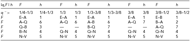
Figure 6 shows the marginal distribution of F for q = 38/111. The above functions are needed because the relative order of various defining points change with changes of q. The distribution of F is defined according to Table 2. For example, when $q = {1 \mathord{\left/ {\vphantom {1 3}} \right. \kern-\nulldelimiterspace} 3}$ , the function is

(22) \begin{equation} \Pi (F) = h_1 ,h_6 ,h_4 ,h_5\end{equation}

over the respective intervals of F: E–A, A–Q, Q–N, and N–V.

TABLE 1

The Coordinates of the Vertices of the Admissible Regions as Functions of q

TABLE 2

Definition of the Marginal Distribution of F for 1/4 < q < 1/2

FIGURE 6

The marginal distribution of F for q = 38/111 (Pr_F stands for probability density of F).

The distribution Π(F) of F has mode (1 − 2q)/(2(1 − q)). This gives the distribution of genotypes:

(23) \begin{equation} \{ f_0 = {q \mathord{\left/ {\vphantom {q 2}} \right. \kern-\nulldelimiterspace} 2},f_1 = q,f_2 = 1 - 3q/2\} .\end{equation}

The Estimation of F

Cavalli-Sforza and Bodmer (1971, p. 43) give data relating to the MN blood-group locus: 47 M, 52 MN, and 12 N individuals. There are 76 N genes from a total 222 and so the frequency of gene N is q = 38/111. These are the counts used to illustrate the estimation method. The method of gene counting is the orthodox method of estimating q. I treat this as the ‘true’ value of q although clearly the value 38/111 is subject to sampling error. The standard error of estimate is available.

Figure 6 displays the (marginal) distribution of F using q = 38/111which I employ as the prior distribution to get the posterior distribution of F shown in Figure 7.

FIGURE 7

The posterior distribution of F computed from genotypic counts {12, 52, 47} from which q = 38/111 (Pr_F stands for probability density of F).

If the value of the fixation index is F, the genotypic proportions in the population are as follows:

(24) \begin{eqnarray} \{ f_0 &=& q^2 + Fpq,\,\,\,f_1 = 2pq - 2Fpq,\,\,\,f_2 = p^2 + Fpq\}.\nonumber\\&&\end{eqnarray}

Denoting the genotypic counts by {n_UU , n_UT , n_TT }, the (conditional) probability of observing these counts is as follows:

(25) \begin{equation} C(F) = \frac{{n!}}{{n_{UU} !\,\, \times n_{UT} !\,\, \times n_{TT} !}} \times f_0^{n_{UU} } \times f_1^{n_{UT} } \times f_2^{n_{TT} } ,\end{equation}

where n is the sample size.

If P(F).dF is the prior probability that F lies in an infinitesimal interval containing F, then, following Thomas Bayes, the posterior probability that it is in that interval is as follows:

(26) \begin{equation} {\rm P'}(F).dF = \frac{{{\rm P}\left( F \right).dF \times C(F)}}{{\int {{\rm P}\left( F \right) \times C(F)} .dF}}.\end{equation}

The posterior distribution of F from (26) for the above counts is displayed in Figure 7.