


1. Introduction
In monopoly insurance markets under perfect information, the classical literature has been mostly interested in characterizing the insurer’s profit-maximizing (or welfare-maximizing) insurance contracts, without any consideration for strategic interaction between the insurer and insured. Whenever such strategic considerations are introduced into the market model, the natural framework is a sequential-move game with the insurer as the leader and the insured as the follower, borrowing from the literature on bilateral monopoly. This is a two-stage game, whereby in the first stage, the insured selects their optimal indemnification given a certain pricing mechanism selected by the insurer; and in the second stage, the insurer observes the insured’s demand function and sets prices so as to maximize profit or welfare. The associated strategic equilibrium concept has been termed the Stackelberg equilibrium (SE), or Bowley optimum.
Bowley optima were first introduced by Bowley (Reference Bowley1928) in the context of a bilateral monopoly and then first applied to insurance markets by Chan and Gerber (Reference Chan and Gerber1985), in the context of expected-utility (EU) preferences with exponential utility functions. Several extensions and/or modifications to this model have subsequently been proposed. For instance, G.Taylor (1992) extends these findings to more general risk exchanges with EU preferences. Cheung et al. (Reference Cheung, Yam and Zhang2019) consider the case of markets in which the insurer is a risk-neutral EU maximizer, who sets premia using a distortion premium principle, and a insured who seeks to minimize a distortion risk measure (DRM). They assume that the insured’s distortion function is either a concave function (indicating risk aversion), or a distortion function corresponding to the value-at-risk (VaR) risk measure. Li and Young (Reference Li and Young2021) characterize Stackelberg equilibria when agents use a mean-variance functional. Boonen et al. (Reference Boonen, Cheung and Zhang2021) and Boonen and Zhang (Reference Boonen and Zhang2022) examine the effect of information asymmetry in the context of DRMs. Ghossoub et al. (Reference Ghossoub, Li and Shi2025) propose an extension in a different direction, by examining the optimal (nonlinear) pricing mechanisms in the market for the class of deductible and coinsurance indemnity functions. Boonen and Ghossoub (Reference Boonen and Ghossoub2023) examine the relationship between Bowley optimality and Pareto optimality, under fairly general preferences. Zhu et al. (Reference Zhu, Ghossoub and Boonen2023) and Ghossoub and Zhu (Reference Ghossoub and Zhu2024) provide the first extensions beyond the case of a two-agent insurance market. The former consider a market with multiple insurer having the first move advantage, and one insured; whereas the latter consider the case of one monopoly insurance facing demand from several policyholders. Andraos et al. (Reference Andraos, Ghossoub and Zhu2026) recently provided a unification and an extension thereof to more general preferences.
Beyond the static framework discussed above, a growing literature has studied Stackelberg equilibria in dynamic settings using stochastic differential game techniques, in which the reinsurer, acting as the leader, and the insurer, acting as the follower, interact sequentially over time. In particular, Chen and Shen (Reference Chen and Shen2018) study a continuous-time Stackelberg reinsurance game in which both parties aim to maximize the expected utility of their terminal wealth. Chen and Shen (Reference Chen and Shen2019) extend this framework to a mean-variance setting. More recent contributions extend this framework to settings involving random horizons, ambiguity aversion, and Lévy risk processes. In particular, Li and Young (Reference Li and Young2022) consider the problem with a random time horizon under the mean-variance principle, while Cao et al. (Reference Cao, Li, Young and Zou2022) study a dynamic Stackelberg game between an ambiguity-averse insurance buyer and seller under the spectrally negative Lévy processes. Cao et al. (Reference Cao, Li, Young and Zou2023b) extend the model of Cao et al. (Reference Cao, Li, Young and Zou2022) to a general divergence penalty for ambiguity. Several extensions also incorporate investment decisions and interactions in stochastic financial markets (e.g., Gu et al., Reference Gu, Viens and Shen2020; Wang and Siu, Reference Wang and Siu2020; Bai et al., Reference Bai, Zhou, Xiao and Gao2021, Reference Bai, Zhou, Xiao, Gao and Zhong2022; Yang et al., Reference Yang, Zhang and Zhu2022), while more recent studies consider dynamic settings with multiple reinsurers (e.g., Chen et al., Reference Chen, Shen and Su2020; Cao et al., Reference Cao, Li, Young and Zou2023a, Reference Cao, Li, Young and Zou2024).
In this paper, we consider a monopoly insurance market with a single policyholder. We assume that the policyholder evaluates insurance contracts using a DRM, following the approach of Assa (Reference Assa2015), Cheung et al. (Reference Cheung, Yam and Zhang2019), or Zhu et al. (Reference Zhu, Ghossoub and Boonen2023), for instance. The insurer is a risk-neutral profit maximizer, who sets premia using a distortion premium principle. To avoid ex post moral hazard that might arise from the policyholder’s misreporting of the true value of the loss, we impose the customary no sabotage condition of Carlier and Dana (Reference Carlier and Dana2003, Reference Carlier and Dana2005) on the set of acceptable indemnity functions. Our framework is most closely related to that of Cheung et al. (Reference Cheung, Yam and Zhang2019). However, in contrast to their study, which assumes that the policyholder is either strictly risk averse (strictly concave distortion function) or a VaR minimizer, we impose no specific restriction on the curvature of the policyholder’s distortion function. This is a significant extension, as it accommodates for several forms of distortion functions that are empirically more relevant than the concave distortion functions, such as the inverse-S-shaped distortion functions of Tversky and Kahneman (Reference Tversky and Kahneman1992), the S-shaped distortion functions of Prelec (Reference Prelec1998), or the very flexible class of distortion functions recently introduced by Bleichrodt et al. (Reference Bleichrodt, Grant and Yang2023).
To characterize Stackelberg equilibria in our model, we proceed in two steps. First for a fixed distortion function used to determine the distortion premium principle, we determine the optimal indemnity function that minimizes the policyholder’s risk measure of their end-of-period risk exposure (Theorem 3.6). Second, using the resulting optimal indemnity, we find the pricing distortion function that maximizes the insurer’s expected profit (Corollary 3.10). We show that, in the first step, the optimal indemnity function exhibits a layer-type structure, determined by the interplay between the policyholder’s distortion function and the insurer’s pricing distortion function. Specifically, the optimal indemnity provides full indemnification over any loss layer on which the policyholder is more pessimistic than the insurer’s pricing functional about tail losses. When the policyholder is less pessimistic than the insurer’s pricing functional about tail losses, no indemnification is offered. Finally, when the policyholder and the insurer’s pricing functional are equally pessimistic about tail losses, the marginal indemnity may take an arbitrary shape, within the global 1-Lispchitz (i.e., comonotonicity) constraints. In the second step, the optimal pricing distortion is determined by the policyholder’s degree of (weak) risk aversion, that is, whether the policyholder’s distortion function is above or below the identity function. In equilibrium, the insurer selects a pricing distortion that is aligned with the policyholder’s risk perception, as encoded by their distortion function, in the sense that prices never exceed the policyholder’s marginal willingness to insure tail losses. Moreover, we show that both the insurance coverage and the insurer’s expected profit increase with the policyholder’s degree of strong or weak risk aversion.
We also analyze the Pareto efficiency of the SE contracts. Our results show that any SE contract is Pareto optimal and makes the policyholder indifferent between participating and not participating in the insurance market. Moreover, any Pareto-optimal contract in which the policyholder is indifferent between participation and non-participation can be obtained at an SE. These findings echo similar results obtained by Boonen and Ghossoub (Reference Boonen and Ghossoub2023) and Ghossoub and Zhu (Reference Ghossoub and Zhu2024), and they highlight a well-known fundamental phenomenon that occurs in monopoly markets, whereby all consumer surplus is extracted by the monopoly.
When the policyholder is either weakly risk averse (with a distortion function that lies above the identity function) or strongly risk averse (with a concave distortion function), we show that the optimal contract provides full insurance, and the optimal pricing distortion function coincides with that of the policyholder. This recovers the result of Cheung et al. (Reference Cheung, Yam and Zhang2019) in the case of concave distortion function. For policyholders who minimize VaR at a confidence level $\alpha \in (0,1)$
, the optimal coverage includes an upper limit. Specifically, the contract provides full insurance for losses below the
$\alpha \in (0,1)$
, the optimal coverage includes an upper limit. Specifically, the contract provides full insurance for losses below the $\alpha$
-quantile while leaving the upper tail uninsured. This recovers another result of Cheung et al. (Reference Cheung, Yam and Zhang2019). However, in contrast, we show that for individuals with inverse-S shaped distortion functions, reflecting strong sensitivity to extreme losses, the optimal indemnity function takes the form of a deductible contract, whereby extreme losses are fully transferred to the insurer.
$\alpha$
-quantile while leaving the upper tail uninsured. This recovers another result of Cheung et al. (Reference Cheung, Yam and Zhang2019). However, in contrast, we show that for individuals with inverse-S shaped distortion functions, reflecting strong sensitivity to extreme losses, the optimal indemnity function takes the form of a deductible contract, whereby extreme losses are fully transferred to the insurer.
The remainder of this paper is organized as follows. Section 2 introduces the insurance market setting, including the risk preferences of the agents, the market mechanisms and resulting insurance contracts, and the (Stackelberg, or Bowley) equilibrium concept. Section 3 provides a characterization of Stackelberg equilibria in our setting. Section 4 examines the Pareto efficiency of the equilibrium contracts and provides a version of the two welfare theorems. Section 5 presents several examples of interest, for specific types of policyholders. Finally, Section 6 concludes. Proofs and related analysis are given in the Appendices.
2. Problem formulation
Let $B(\mathcal{F})$
denote the set of all bounded random variables on a given non-atomic probability space
$B(\mathcal{F})$
denote the set of all bounded random variables on a given non-atomic probability space $(\Omega,\mathcal{F},\mathbb{P})$
. An individual, or potential policyholder, is subject to an insurable loss, which we model as a random variable
$(\Omega,\mathcal{F},\mathbb{P})$
. An individual, or potential policyholder, is subject to an insurable loss, which we model as a random variable $X \in B^+(\mathcal{F})$
, the positive cone of
$X \in B^+(\mathcal{F})$
, the positive cone of $B(\mathcal{F})$
, with range [0, M]. A positive realization of X is seen as a loss. We denote by
$B(\mathcal{F})$
, with range [0, M]. A positive realization of X is seen as a loss. We denote by $F_X$
the cumulative distribution function (CDF) of X, and by
$F_X$
the cumulative distribution function (CDF) of X, and by $F_X^{-1}$
the left-continuous inverse of
$F_X^{-1}$
the left-continuous inverse of $F_X$
, i.e., the quantile of X, defined as:
$F_X$
, i.e., the quantile of X, defined as:
 \begin{equation*}F_X^{-1}(t) =\inf\left\{z\in\mathbb{R}^+ \, \middle| \, F_X(z)\ge t\right\},\quad \forall t\in[0,1].\end{equation*}
Let $\mathcal{Q}$
denote the set of quantile functions of random variables in
$\mathcal{Q}$
denote the set of quantile functions of random variables in $B(\mathcal{F})$
. That is,
$B(\mathcal{F})$
. That is,
 \begin{equation*}\mathcal{Q} =\left\{q\,:\,(0,1)\to\mathbb{R}^+\,\middle|\,q \mbox{ is nondecreasing and left-continuous}\right\}.\end{equation*}
2.1. Preferences
Definition 2.1. A DRM $\rho$
on
$\rho$
on $(\Omega,\mathcal{F},\mathbb{P})$
is defined as the Choquet integral with respect to the distorted probability measure
$(\Omega,\mathcal{F},\mathbb{P})$
is defined as the Choquet integral with respect to the distorted probability measure $T \circ \mathbb{P}$
. Namely, for any
$T \circ \mathbb{P}$
. Namely, for any $Y \in B(\mathcal{F})$
,
$Y \in B(\mathcal{F})$
,
 \begin{align*}\rho(Y)=\int\, Y\,\mathrm{d}T\circ\mathbb{P}= \int_0^{+\infty}T(\mathbb{P}(Y\geq y))\,\mathrm{d}y + \int_{-\infty}^0 \left[T(\mathbb{P}(Y\geq y))-1\right]\mathrm{d}y,\end{align*}
where $T\,:\,[0,1]\rightarrow[0,1]$
is a distortion function, that is, a nondecreasing differentiable mapping, satisfying
$T\,:\,[0,1]\rightarrow[0,1]$
is a distortion function, that is, a nondecreasing differentiable mapping, satisfying $T(0)=0$
and
$T(0)=0$
and $T(1)=1$
.
$T(1)=1$
.
The conjugate of the distortion function T is given by: $\widetilde T (t)= 1 - T(1-t)$
, for all
$\widetilde T (t)= 1 - T(1-t)$
, for all $t \in [0,1]$
. It is easy to verify that
$t \in [0,1]$
. It is easy to verify that $\widetilde T$
is a distortion function.
$\widetilde T$
is a distortion function.
The policyholder’s preference over $B(\mathcal F)$
is assumed to admit a DRM representation, associated with a distortion function T. Specifically, for any
$B(\mathcal F)$
is assumed to admit a DRM representation, associated with a distortion function T. Specifically, for any $Z \in B(\mathcal F)$
, the policyholder evaluates risk according to
$Z \in B(\mathcal F)$
, the policyholder evaluates risk according to
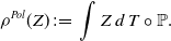 \begin{equation}\rho^{Pol}(Z) \,:\!=\, \int Z \, d \,T \circ \mathbb P.\end{equation}
The induced preference relation $\succcurlyeq$
on
$\succcurlyeq$
on $B(\mathcal F)$
is defined by
$B(\mathcal F)$
is defined by $ Z_1 \succcurlyeq Z_2$
, if and only if,
$ Z_1 \succcurlyeq Z_2$
, if and only if, $\rho^{\mathrm{Pol}}(Z_1) \le \rho^{\mathrm{Pol}}(Z_2)$
. Indifference is defined by
$\rho^{\mathrm{Pol}}(Z_1) \le \rho^{\mathrm{Pol}}(Z_2)$
. Indifference is defined by $Z_1 \sim Z_2$
, whenever
$Z_1 \sim Z_2$
, whenever $Z_1 \succcurlyeq Z_2$
, and
$Z_1 \succcurlyeq Z_2$
, and $Z_2 \succcurlyeq Z_1$
.
$Z_2 \succcurlyeq Z_1$
.
2.2. Risk aversion
Given two random variables $Z_1, Z_2 \in B (\mathcal{F})$
, we say that
$Z_1, Z_2 \in B (\mathcal{F})$
, we say that $Z_1$
dominates
$Z_1$
dominates $Z_2$
in second-order stochastic dominance (SSD), written
$Z_2$
in second-order stochastic dominance (SSD), written $Z_1 \succcurlyeq_{_{SSD}} Z_2$
, if
$Z_1 \succcurlyeq_{_{SSD}} Z_2$
, if
 \begin{equation*}\displaystyle \int_{-\infty}^{x}F_{Z_1}(t) \ dt \leq \int_{-\infty}^{x} F_{Z_2}(t) \ dt, \quad \text{for all $x \in \mathbb{R}$}.\end{equation*}
Moreover, $Z_2$
is said to be a mean-preserving increase in risk (MPIR) of
$Z_2$
is said to be a mean-preserving increase in risk (MPIR) of $Z_1$
if
$Z_1$
if $\mathbb{E}[Z_1] = \mathbb{E}[Z_2]$
and
$\mathbb{E}[Z_1] = \mathbb{E}[Z_2]$
and $Z_1 \succcurlyeq_{ _{SSD}} Z_2$
. We next discuss weak and strong risk aversion of a preference
$Z_1 \succcurlyeq_{ _{SSD}} Z_2$
. We next discuss weak and strong risk aversion of a preference $\succcurlyeq$
over
$\succcurlyeq$
over $B(\mathcal{F})$
.
$B(\mathcal{F})$
.
Definition 2.2. A preference $\succcurlyeq$
over
$\succcurlyeq$
over $B(\mathcal{F})$
is said to be weakly risk averse, if
$B(\mathcal{F})$
is said to be weakly risk averse, if $\mathbb{E}[Z] \succcurlyeq Z$
for all
$\mathbb{E}[Z] \succcurlyeq Z$
for all $Z \in B(\mathcal{F})$
.
$Z \in B(\mathcal{F})$
.
Definition 2.3. A preference $\succcurlyeq$
over
$\succcurlyeq$
over $B(\mathcal{F})$
is said to be strongly risk averse if it ranks any random variable above all of its mean-preserving increases in risk. That is,
$B(\mathcal{F})$
is said to be strongly risk averse if it ranks any random variable above all of its mean-preserving increases in risk. That is, $\succcurlyeq$
is strongly risk averse if
$\succcurlyeq$
is strongly risk averse if $Z_1 \succcurlyeq Z_2$
, for all
$Z_1 \succcurlyeq Z_2$
, for all $ Z_1, Z_2 \in B(\mathcal{F})$
, such that
$ Z_1, Z_2 \in B(\mathcal{F})$
, such that $Z_2$
is an MPIR of
$Z_2$
is an MPIR of $Z_1$
.
$Z_1$
.
Strong risk aversion implies weak risk aversion, since any $Z\in B(\mathcal F)$
is a mean-preserving increase in risk of
$Z\in B(\mathcal F)$
is a mean-preserving increase in risk of $\mathbb{E}[Z]$
. Moreover, by the positive homogeneity of the Choquet integral, it follows that
$\mathbb{E}[Z]$
. Moreover, by the positive homogeneity of the Choquet integral, it follows that
 \begin{equation*}\mathbb{E}[Z] \succcurlyeq Z \Longleftrightarrow \mathbb{E}[Z] \leq \rho^{Pol}(Z), \quad \forall Z \in B(\mathcal{F}).\end{equation*}
By a classical result (see, e.g., Yaari, Reference Yaari1987), risk aversion under DRM is characterized by properties of the distortion function T. In particular, the policyholder is weakly risk averse if and only if $T(t) \geq t$
for all
$T(t) \geq t$
for all $t\in[0,1]$
. Moreover, the policyholder is strongly risk averse if and only if the distortion function T is concave.
$t\in[0,1]$
. Moreover, the policyholder is strongly risk averse if and only if the distortion function T is concave.
Recall that for a given preference relation $\succcurlyeq$
, the certainty equivalent of
$\succcurlyeq$
, the certainty equivalent of $Z \in B(\mathcal{F})$
is the constant
$Z \in B(\mathcal{F})$
is the constant $\text{CE}^\succcurlyeq(Z) \in \mathbb{R}$
such that
$\text{CE}^\succcurlyeq(Z) \in \mathbb{R}$
such that
 \begin{equation*}Z \sim \text{CE}^\succcurlyeq(Z),\end{equation*}
and the risk premium associated with $Z \in B(\mathcal{F})$
is defined as
$Z \in B(\mathcal{F})$
is defined as
 \begin{equation*}\Delta^\succcurlyeq(Z) \,:\!=\, \mathbb{E}[Z] - \text{CE}^\succcurlyeq(Z).\end{equation*}
Following Chew et al. (Reference Chew, Karni and Safra1987), Quiggin (Reference Quiggin1993), and Ghossoub and He (Reference Ghossoub and He2021), we define comparative notions of risk aversion below.
Definition 2.4 (Comparative risk aversion). Consider two preference relations $\succcurlyeq$
and
$\succcurlyeq$
and $\succcurlyeq^*$
over
$\succcurlyeq^*$
over $B(\mathcal{F})$
:
$B(\mathcal{F})$
:
-
(1) $\succcurlyeq^*$
is said to be more weakly risk averse than
$\succcurlyeq$
if, for any
$Z \in B(\mathcal{F})$
,
$\Delta^{\succcurlyeq^*}(Z) \geq \Delta^\succcurlyeq(Z)$
.
$\succcurlyeq^*$
is said to be more weakly risk averse than
$\succcurlyeq$
if, for any
$Z \in B(\mathcal{F})$
,
$\Delta^{\succcurlyeq^*}(Z) \geq \Delta^\succcurlyeq(Z)$
. -
(2)
$\succcurlyeq^*$
is said to be more strongly risk averse than
$\succcurlyeq$
if
$Z_1 \succcurlyeq^* Z_2$
for any
$Z_1, Z_2 \in B(\mathcal{F})$
such that:-
(a)
$Z_1 \sim Z_2$
. -
(b) There exists
$z_0 \in \mathbb{R}$
with
$F_{Z_2}(z) \geq F_{Z_1}(z)$
for all
$z \lt z_0$
, and
$F_{Z_2}(z) \leq F_{Z_1}(z)$
for all
$z \geq z_0$
.
-





By a classical result (e.g., Chew et al., Reference Chew, Karni and Safra1987), we obtain the following characterization of comparative weak and strong risk aversion for DRMs.
Proposition 2.5. Consider two policyholders whose preferences $\succcurlyeq$
and
$\succcurlyeq$
and $\succcurlyeq^*$
over
$\succcurlyeq^*$
over $B(\mathcal{F})$
admit representations by DRMs
$B(\mathcal{F})$
admit representations by DRMs $\rho^{Pol}$
and
$\rho^{Pol}$
and ${\rho^{*}}^{Pol}$
, respectively. Let T and
${\rho^{*}}^{Pol}$
, respectively. Let T and $T^*$
denote the respective distortion functions of each policyholder. Then, the following holds:
$T^*$
denote the respective distortion functions of each policyholder. Then, the following holds:
-
(1) The second policyholder is more weakly risk averse than the first policyholder if and only if
$T^*(t) \geq T(t)$
, for all
$t \in [0,1]$
. -
(2) The second policyholder is more strongly risk averse than the first policyholder if and only if
$T^*$
is a concave transformation of T. That is, there exists an increasing and concave function
$g: [0,1] \to [0,1]$
, satisfying
$g(0) = 0$
,
$g(1) = 1$
, and
$T^*(t) = g\left(T(t)\right)$
for all
$t \in [0,1]$
.







Remark 2.6. If g is an increasing and concave function on [0,1] such that $g(0)=0$
and
$g(0)=0$
and $g(1)=1$
, then
$g(1)=1$
, then $g(t) \geq t$
, for all
$g(t) \geq t$
, for all $t \in [0,1]$
. Consequently, if
$t \in [0,1]$
. Consequently, if $T^* \equiv g \circ T$
, we obtain that
$T^* \equiv g \circ T$
, we obtain that $T^*(t) \geq T(t)$
for all
$T^*(t) \geq T(t)$
for all $t \in [0,1]$
. That is, if
$t \in [0,1]$
. That is, if $T^*$
is more strongly risk averse than T, then
$T^*$
is more strongly risk averse than T, then $T^*$
is also more weakly risk averse than T.
$T^*$
is also more weakly risk averse than T.
2.3. Market mechanisms and contracts
The market allows the policyholder to cede part of the loss X to an insurer, in exchange for a premium payment. We assume that the market only offers indemnities in the set of ex ante admissible indemnity schedules $\mathcal{I}_L$
defined below.
$\mathcal{I}_L$
defined below.
 \begin{equation*}\mathcal{I}_L = \big\{I\,:\, [0,M]\rightarrow [0,M] \ \big\vert \ I(0)=0, \ 0\leq I(x_1)- I(x_2)\leq x_1-x_2, \forall\, x_2\leq x_1 \in [0,M]\big\}.\end{equation*}
That is, $\mathcal{I}_L$
is the set of 1-Lipschitz functions satisfying the so-called no-sabotage condition of Carlier and Dana (Reference Carlier and Dana2003), so as to rule ex post moral hazard that could arise from misreporting of the actual realized loss.
$\mathcal{I}_L$
is the set of 1-Lipschitz functions satisfying the so-called no-sabotage condition of Carlier and Dana (Reference Carlier and Dana2003), so as to rule ex post moral hazard that could arise from misreporting of the actual realized loss.
Definition 2.7. An insurance contract is a pair $(I,\pi)$
, where
$(I,\pi)$
, where $I \in \mathcal{I}_L$
is an indemnity function and
$I \in \mathcal{I}_L$
is an indemnity function and $\pi\in\mathbb{R}$
is the premium paid by the policyholder for coverage I.
$\pi\in\mathbb{R}$
is the premium paid by the policyholder for coverage I.
Assumption 2.8. The insurer is assumed to price insurance using a distortion premium principle of the form:
 \begin{align}\Pi_g\left(I(X)\right)\,:\!=\, \int I(X) \, d g \circ \mathbb{P}, \quad \forall \, I \in \mathcal{I}_L,\end{align}
for some distortion function g, which we hereafter refer to as the pricing distortion used by the insurer.
Definition 2.9. A market mechanism is a pair (I,g), where $I \in \mathcal{I}_L$
is an indemnity function and g is a pricing distortion function.
$I \in \mathcal{I}_L$
is an indemnity function and g is a pricing distortion function.
A market mechanism (I,g) induces an insurance contract of the form $(I,\Pi_g ( I(X) ))$
, where the premium is computed using the pricing distortion g. The insurer’s end-of-period profit is therefore given by
$(I,\Pi_g ( I(X) ))$
, where the premium is computed using the pricing distortion g. The insurer’s end-of-period profit is therefore given by $\Pi_g ( I(X) ) - I(X)$
, while the policyholder’s end-of-period risk exposure is given by
$\Pi_g ( I(X) ) - I(X)$
, while the policyholder’s end-of-period risk exposure is given by $X-I(X) + \Pi_g ( I(X) )$
. Accordingly, the insurer’s resulting expected profit is
$X-I(X) + \Pi_g ( I(X) )$
. Accordingly, the insurer’s resulting expected profit is
 \begin{align}V^{In}(I,g) = \Pi_g \big( I(X) \big) -\mathbb{E}\left[I(X)\right],\end{align}
and the policyholder evaluates this risk exposure using:
 \begin{align}\rho^{Pol}(I,g)= \rho^{Pol} ( X - I(X) + \Pi_g ( I(X) ) ).\end{align}
Letting $R(X) \,:\!=\, X - I(X)$
denote the retention function, i.e., the part of the loss X that is retained by the policyholder, and by translation invariance of
$R(X) \,:\!=\, X - I(X)$
denote the retention function, i.e., the part of the loss X that is retained by the policyholder, and by translation invariance of $\rho^{Pol}$
, (4) reduces to:
$\rho^{Pol}$
, (4) reduces to:
 \begin{equation}\rho^{Pol}(I,g)=\rho^{Pol}( R(X) ) + \Pi_g ( I(X) ).\end{equation}
Remark 2.10. An indemnity function I belongs to $\mathcal I_L$
if and only if the corresponding retention function
$\mathcal I_L$
if and only if the corresponding retention function $R(X)=X-I(X)$
belongs to
$R(X)=X-I(X)$
belongs to $\mathcal I_L$
. Moreover, since I is nondecreasing, the random variables I(X) and R(X) are comonotonic.Footnote 1
$\mathcal I_L$
. Moreover, since I is nondecreasing, the random variables I(X) and R(X) are comonotonic.Footnote 1
2.4. A sequential-move game
The insurance market is modeled as a sequential-move game, in which the insurer, having the first-mover advantage, starts by selecting a pricing distortion function g. Given that choice, the policyholder then selects an indemnity function that minimizes their risk exposure $\rho^{Pol}(I,g)$
. Anticipating the policyholder’s optimal indemnity choice as a function of the selected pricing distortion function g, the insurer selects the optimal distortion function
$\rho^{Pol}(I,g)$
. Anticipating the policyholder’s optimal indemnity choice as a function of the selected pricing distortion function g, the insurer selects the optimal distortion function $g^*$
that maximizes their expected profit
$g^*$
that maximizes their expected profit $V^{In}(I,g)$
. The equilibrium concept that is best suited for this sequential game is the SE.
$V^{In}(I,g)$
. The equilibrium concept that is best suited for this sequential game is the SE.
Definition 2.11. A given market mechanism $( I^*,g^*) $
is said to be an SE, if
$( I^*,g^*) $
is said to be an SE, if
-
(1)
$I^* \in \underset{I \in \mathcal{I}_L} {\arg\min} \ \rho^{Pol}( I,{g^*})$
, and -
(2)
$V^{In}(I^*,{g^*}) \geq V^{In}( I,g)$
, for all (I,g) such that
$ I\in \underset{\bar I \in \mathcal{I}_L}{\arg\min} \ \rho^{Pol}( \bar I,g)$
.


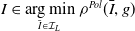
Definition 2.11 suggests that Stackelberg equilibria can be characterized through a two-step procedure. In the first step, for a fixed pricing distortion function g, the policyholder chooses an indemnity function that minimizes their risk exposure. This problem will be referred to as the policyholder’s problem. In the second step, anticipating the policyholder’s optimal response as a function of g, the insurer selects a pricing distortion function $g^*$
that maximizes expected profit. This problem will be referred to as the insurer’s problem.
$g^*$
that maximizes expected profit. This problem will be referred to as the insurer’s problem.
For a given insurance contract $(I,\pi) \in \mathcal{I}_L \times \mathbb{R}$
, the policyholder’s risk exposure and the insurer’s expected profit can be written as
$(I,\pi) \in \mathcal{I}_L \times \mathbb{R}$
, the policyholder’s risk exposure and the insurer’s expected profit can be written as
 \begin{equation*}{\rho}^{Pol}(I,\pi) = {\rho}^{Pol}(X-I(X)+\pi)\quad \hbox{ and }\quad {V}^{In}(I,\pi)=\pi -\mathbb{E}[I(X)].\end{equation*}
Definition 2.12. An insurance contract $(I^*,\pi^*) \in \mathcal{I}_L \times \mathbb{R}$
is said to be individually rational, IR, if
$(I^*,\pi^*) \in \mathcal{I}_L \times \mathbb{R}$
is said to be individually rational, IR, if
 \begin{equation*}\rho^{Pol}(I^*,\pi^*) \leq \rho^{Pol}(0,0)\quad \hbox{ and } \quad V^{In}(I^*,\pi^*) \geq V^{In}(0,0).\end{equation*}
Definition 2.12 states that an insurance contract $(I^*,\pi^*) \in \mathcal{I}_L \times \mathbb{R}$
is individually rational, if it incentivizes the policyholder and the monopolist insurer to participate in the market.
$(I^*,\pi^*) \in \mathcal{I}_L \times \mathbb{R}$
is individually rational, if it incentivizes the policyholder and the monopolist insurer to participate in the market.
Definition 2.13. An insurance contract $(I^*,\pi^*) \in \mathcal{I}_L \times \mathbb{R}$
is said to be Pareto optimal, PO, if there does not exist another contract
$(I^*,\pi^*) \in \mathcal{I}_L \times \mathbb{R}$
is said to be Pareto optimal, PO, if there does not exist another contract $(I,\pi) \in \mathcal{I}_L \times \mathbb{R}$
such that
$(I,\pi) \in \mathcal{I}_L \times \mathbb{R}$
such that
 \begin{equation*}\rho^{Pol}(I,\pi) \leq \rho^{Pol}(I^*,\pi^*)\quad \hbox{ and } \quad V^{In}(I,\pi) \geq V^{In}(I^*,\pi^*),\end{equation*}
with at least one strict inequality.
Definition 2.13 states that an insurance contract $(I^*,\pi^*) \in \mathcal{I}_L \times \mathbb{R}$
is Pareto optimal if there is no alternative contract that weakly reduces the policyholder’s risk exposure and weakly increases the insurer’s profit, with at least one of these improvements being strict.
$(I^*,\pi^*) \in \mathcal{I}_L \times \mathbb{R}$
is Pareto optimal if there is no alternative contract that weakly reduces the policyholder’s risk exposure and weakly increases the insurer’s profit, with at least one of these improvements being strict.
3. Characterization of Stackelberg equilibria
In this section, we aim to characterize Stackelberg equilibria through a two-step procedure as suggested in Definition 2.11. Specifically, in Subsection 3.1, we study the policyholder’s problem, which constitutes the first step in determining Stackelberg equilibria. Then, in Subsection 3.2, we consider the second step by addressing the insurer’s problem.
3.1. The policyholder’s problem
For a given choice of pricing distortion function g, the policyholder chooses an indemnity $I \in \mathcal{I}_L$
to minimize risk exposure:
$I \in \mathcal{I}_L$
to minimize risk exposure:
 \begin{align}\min\limits_{I\in \mathcal{I}_L} \, \rho^{Pol}(I,g).\end{align}
To analyze the policyholder’s problem given in (6), we impose the following assumption on the loss distribution that will allow us to reformulate the problem in terms of quantile functions.
Assumption 3.1. The cumulative distribution function $F_X$
is strictly increasing.
$F_X$
is strictly increasing.
It follows from Assumption 3.1 that $F_X$
is differentiable almost everywhere. Moreover, by Föllmer and Schied (Reference Föllmer and Schied2016, Lemma A.25), Assumption 3.1 also guarantees that
$F_X$
is differentiable almost everywhere. Moreover, by Föllmer and Schied (Reference Föllmer and Schied2016, Lemma A.25), Assumption 3.1 also guarantees that $U \,:\!=\, F_X(X)$
is uniformly distributed on (0,1) and that
$U \,:\!=\, F_X(X)$
is uniformly distributed on (0,1) and that $X=F_X^{-1}(U), \ \mathbb{P}$
-a.s.
$X=F_X^{-1}(U), \ \mathbb{P}$
-a.s.
Remark 3.2. For each $I \in \mathcal{I}_L$
, I(X) and
$I \in \mathcal{I}_L$
, I(X) and $X-I(X)$
have strictly increasing CDF by Assumption 3.1. Consequently, their quantile functions are strictly increasing, left-continuous, and differentiable a.e. on [0,1].
$X-I(X)$
have strictly increasing CDF by Assumption 3.1. Consequently, their quantile functions are strictly increasing, left-continuous, and differentiable a.e. on [0,1].
For any $Z \in B^+(\mathcal{F})$
whose quantile function
$Z \in B^+(\mathcal{F})$
whose quantile function $F_Z^{-1}$
is differentiable almost everywhere, the policyholder’s risk measure admits the following representation:
$F_Z^{-1}$
is differentiable almost everywhere, the policyholder’s risk measure admits the following representation:
 \begin{align*}\rho^{Pol}(Z)&=\int\, Z \,\mathrm{d}T\circ\mathbb{P}=\int \left(F_Z^{-1}\right)^{\prime}(U) \, T(1-U)\,\mathrm{d}\mathbb{P}.\end{align*}
Similarly, the premium evaluated under the given pricing distortion g can be written as
 \begin{align*}\Pi_g\left(Z\right)=\int Z \, d g \circ \mathbb{P}=\int \left(F_Z^{-1}\right)^{\prime}(U) \, g(1-U)\,\mathrm{d}\mathbb{P}.\end{align*}
Applying these formulas to the retention R(X) and the indemnity I(X), respectively, and using expression (5) of $\rho^{\mathrm{Pol}}(I,g)$
, we obtain
$\rho^{\mathrm{Pol}}(I,g)$
, we obtain
 \begin{equation}\rho^{Pol}(I,g)=\int \left(F_{R(X)}^{-1}\right)^{\prime}(U) \ T(1-U)\,\mathrm{d}\mathbb{P}+\int \left(F_{I(X)}^{-1}\right)^{\prime}(U) \ g(1-U)\,\mathrm{d}\mathbb{P}.\end{equation}
Remark 3.3. Since $X = I(X) + R(X)$
, we can write
$X = I(X) + R(X)$
, we can write $F_X^{-1} = F_{I(X)}^{-1} + F_{R(X)}^{-1}$
, by comonotonic additivity of the quantile function.
$F_X^{-1} = F_{I(X)}^{-1} + F_{R(X)}^{-1}$
, by comonotonic additivity of the quantile function.
As a result of the above remark, (7) can be rewritten as follows:
 \begin{align*}\rho^{Pol}(I,g)&=\int_0^1 \left(F_{R(X)}^{-1}\right)^{\prime}(t) \ \left[T(1-t) - g(1-t)\right]\mathrm{d}t+\int_0^1 \left(F_{X}^{-1}\right)^{\prime}(t)\ g(1-t)\mathrm{d}t.\end{align*}
Let $\mathcal{Q}_L$
be the set of admissible quantile functions, defined as
$\mathcal{Q}_L$
be the set of admissible quantile functions, defined as
 \begin{equation*}\mathcal{Q}_L=\big\{q \in \mathcal{Q}\, \big |\,q(0)=0, \ 0\leq q^{\prime}(t)\leq \left(F_X^{-1}\right)^{\prime}(t)\big\}.\end{equation*}
Each $q \in \mathcal Q_L$
corresponds to the quantile of the retention random variable
$q \in \mathcal Q_L$
corresponds to the quantile of the retention random variable $R(X)=X-I(X)$
for some admissible
$R(X)=X-I(X)$
for some admissible $I \in \mathcal I_L$
. Hence, for a given
$I \in \mathcal I_L$
. Hence, for a given $q \in \mathcal{Q}_L$
, we have
$q \in \mathcal{Q}_L$
, we have
 \begin{align}\rho^{Pol}(q,g)&=\int_0^1 q^{\prime}(t) \, \left[T(1-t) - g(1-t)\right]\,\mathrm{d}t + \int_0^1 \left(F_{X}^{-1}\right)^{\prime}(t) \, g(1-t)\,\mathrm{d}t.\end{align}
Reformulating the policyholder’s problem (6) in quantile form, we obtain
 \begin{align}\min\limits_{q\in \mathcal{Q}_L} \rho^{Pol}( q,g).\end{align}
Lemma 3.4. For a given pricing distortion function g, the feasible quantile $q_{g}(t) \in \mathcal{Q}_L$
is optimal for (9) if and only if the indemnity
$q_{g}(t) \in \mathcal{Q}_L$
is optimal for (9) if and only if the indemnity $I_g(x)= x - q_g \left(F_X(x)\right)$
is optimal for (6).
$I_g(x)= x - q_g \left(F_X(x)\right)$
is optimal for (6).
Proof. The proof can be found in Appendix A.1.
Lemma 3.5. For a given pricing distortion function g, a quantile function $q_g$
is optimal for (9) if and only if
$q_g$
is optimal for (9) if and only if
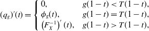 \begin{equation}(q_{{g}})^{\prime}(t)=\left\{\begin{array}[c]{l@{\quad}l} 0, &g(1-t)\lt T(1-t), \\ \phi_{ g}(t), & g(1-t)=T(1-t), \\ \left(F_X^{-1}\right)^{\prime}(t), & g(1-t)\gt T(1-t),\end{array}\right.\end{equation}
where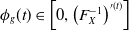 $\phi_g(t)\in\left[0,\left(F_X^{-1}\right)^{\prime(t)}\right]$
, for almost every
$\phi_g(t)\in\left[0,\left(F_X^{-1}\right)^{\prime(t)}\right]$
, for almost every $t \in [0,1]$
such that
$t \in [0,1]$
such that $g(1-t)=T(1-t)$
.
$g(1-t)=T(1-t)$
.
Proof. The proof can be found in Appendix A.2.
Theorem 3.6. For a given pricing distortion function g, an indemnity function $I_g$
is optimal for the policyholder’s problem given in (6) if and only if it is of the form
$I_g$
is optimal for the policyholder’s problem given in (6) if and only if it is of the form $I_g(x) = \int_0^x \kappa(y) \, dy$
, for all
$I_g(x) = \int_0^x \kappa(y) \, dy$
, for all $x \in [0,M]$
, with
$x \in [0,M]$
, with $\kappa: [0,M] \to [0,1]$
satisfying the following:
$\kappa: [0,M] \to [0,1]$
satisfying the following:
 \begin{equation*}\kappa(y) =\left\{\begin{array}[c]{l@{\quad}l} 1, & g\left(\mathbb{P}[X \gt y]\right) \lt T\left(\mathbb{P}[X \gt y]\right), \\1 - \phi_{g}(F_X(y)) \, f_X(y) , & g\left(\mathbb{P}[X \gt y]\right) = T\left(\mathbb{P}[X \gt y]\right), \\0, & g\left(\mathbb{P}[X \gt y]\right) \gt T\left(\mathbb{P}[X \gt y]\right),\end{array}\right.\end{equation*}
where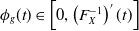 $\phi_g(t)\in\left[0,\left(F_X^{-1}\right)^{\prime}(t)\right]$
, for almost every
$\phi_g(t)\in\left[0,\left(F_X^{-1}\right)^{\prime}(t)\right]$
, for almost every $t \in [0,1]$
such that
$t \in [0,1]$
such that $ g(1-t) = T(1-t)$
, and
$ g(1-t) = T(1-t)$
, and $f_X$
denotes the probability density function of the loss X.
$f_X$
denotes the probability density function of the loss X.
Theorem 3.6 characterizes the set of optimal indemnity functions for a given pricing distortion function g, in terms of the policyholder’s marginal indemnification. Specifically, full indemnification is optimal when the insurer’s pricing distortion assigns less weight to tail probabilities than the policyholder’s distortion function T. The policyholder retains the entire loss if the insurer’s pricing distortion overweights the tail probability compared to the policyholder’s distortion. Finally, when the policyholder’s distortion is equal to the insurer’s pricing distortion at a given tail probability, the policyholder may receive partial coverage, as long as feasibility is maintained.
This structural characterization is consistent with Assa (Reference Assa2015), who considers a reinsurance problem in which the premium principle is fixed and distortion based, and characterizes the optimal contract of the policyholder. In contrast, our result arises as the policyholder’s best response within a Stackelberg framework, where the pricing distortion is a strategic choice of the insurer. Moreover, in the absence of strategic interaction and when the policyholder’s problem only is considered, our model reduces to the setting analyzed in Assa (Reference Assa2015).
3.2. The insurer’s problem
The optimal indemnity characterized in Theorem 3.6 is not unique. The insurer’s objective is to identify a market mechanism $(I^*_{g^*},g^*)$
that solves the following problem:
$(I^*_{g^*},g^*)$
that solves the following problem:
 \begin{align}\max_g \, V^{In}(I_g,g),\ \text{such that} \ I_g \in \arg\min_{I\in\mathcal I_L} \, \rho^{Pol}(I,g).\end{align}
Lemma 3.7. The market mechanism $(I^*_{g^*},g^*)$
is an SE if and only if it is optimal for the insurer’s problem in (11).
$(I^*_{g^*},g^*)$
is an SE if and only if it is optimal for the insurer’s problem in (11).
Proof. The proof follows immediately from Definition 2.11.
The insurer’s problem (11) can be reformulated using quantile functions, similarly to the policyholder’s problem analyzed in Subsection 3.1. Consider a market mechanism (I,g), using Remark 3.3, the premium can be written as
 \begin{equation*}\Pi_g \big( I(X) \big)=\int_0^1 \left[\left(F_{X}^{-1}\right)^{\prime}(t) - \left(F_{R(X)}^{-1}\right)^{\prime}(t)\right]\, g(1-t)\,\mathrm{d}t.\end{equation*}
Moreover,
 \begin{align*}\mathbb{E}\left[I(X)\right]&=\int_0^1 \left[F_{X}^{-1}(t) - F_{R(X)}^{-1}(t) \right] \,\mathrm{d}t.\end{align*}
Substituting the quantile representations of the premium and the expected indemnity into $V^{In}( I_g,g)$
in (3), where
$V^{In}( I_g,g)$
in (3), where $R_g$
denotes the retention function associated with
$R_g$
denotes the retention function associated with $I_g$
, yields:
$I_g$
, yields:
 \begin{align*}V^{In}( I_g,g)&=\int_0^1 \left[\left(F_{X}^{-1}\right)^{\prime}(t) - \left(F_{R_g(X)}^{-1}\right)^{\prime}(t)\right]\, g(1-t)\,\mathrm{d}t-\int_0^1 \left[F_{X}^{-1}(t) - F_{R_g(X)}^{-1}(t)\right]\,\mathrm{d}t.\end{align*}
For a given quantile $q \in \mathcal{Q}_L$
, this expression reduces to:
$q \in \mathcal{Q}_L$
, this expression reduces to:
 \begin{align*}V^{In}(q,g)&=\int_0^1 \left[\left(F_{X}^{-1}\right)^{\prime}(t) - q^{\prime}(t)\right]\, g(1-t)\,\mathrm{d}t-\int_0^1 \left[F_{X}^{-1}(t) - q(t)\right]\,\mathrm{d}t.\end{align*}
Hence, the insurer’s problem can be equivalently written in quantile form as follows:
 \begin{align}\max\limits_{g} \, V^{In}( q_g,g), \quad \text{such that $q_g \in \arg\min_{q \in \mathcal Q_L} \rho^{Pol}(q,g)$}.\end{align}
The following result suggests that solving the insurer’s problem (11) is equivalent to solving (12), providing a one-to-one correspondence between optimal solutions in the quantile space and optimal mechanisms.
Lemma 3.8. $(q_g,g)$
is optimal for (12) if and only if
$(q_g,g)$
is optimal for (12) if and only if $(I_g,g)$
is optimal for (11), where
$(I_g,g)$
is optimal for (11), where $I_g(x) =$ $x - q_g\left(F_X(x)\right)$
, for all
$x - q_g\left(F_X(x)\right)$
, for all $x \in [0,M]$
.
$x \in [0,M]$
.
Proof. The proof is similar to that of Lemma 3.4.
Theorem 3.9. $(q^*_{g^*},{g}^*)$
is optimal for (12) if and only if the following two conditions hold:
$(q^*_{g^*},{g}^*)$
is optimal for (12) if and only if the following two conditions hold:
-
(1) The optimal pricing distortion
$g^*$
satisfies
$g^*(t)=1-\widetilde{g} ^*(1-t)$
for all
$t \in [0,1]$
, where the optimal pricing conjugate
$\widetilde g ^*$
is given by: (13)
\begin{equation}\widetilde g^*(t) = \left\{\begin{array}[c]{l@{\quad}l} \widetilde T(t), &\widetilde T(t)\lt t, \\ \in\left[\,\sup \left\{z \lt t;\ \widetilde g^*(z) \right\}, \widetilde T(t)\right], & \widetilde T(t)\geq t,\end{array}\right.\end{equation}





and $\widetilde T$
is the conjugate distortion function of T.
$\widetilde T$
is the conjugate distortion function of T.
-
(2) The optimal quantile
$q^*_{g^*}$
satisfies: (14)
\begin{equation}\left(q^*_{{g}^*}\right)^{\prime}(t)=\left\{\begin{array}[c]{l@{\quad}l} 0, &\widetilde T(t)\lt t, \\ \phi_{ g^*}(t)\, & t\in\{z; \ \widetilde{g}^*(z)= \widetilde T(z)=z\}, \\ \left(F_X^{-1}\right)^{\prime}(t), &t\in\{z; \ \widetilde{g}^*(z)\lt \widetilde T(z)=z\}\cup\{z; \ \widetilde T(z)\gt z\},\end{array}\right.\end{equation}


where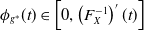 $\phi_{g^*}(t)\in\left[0,\left(F_X^{-1}\right)^{\prime}(t)\right]$
for a.e.
$\phi_{g^*}(t)\in\left[0,\left(F_X^{-1}\right)^{\prime}(t)\right]$
for a.e. $t\in[0,1]$
such that
$t\in[0,1]$
such that $\widetilde{g}^*(t)= \widetilde T(t)=t.$
Moreover, the insurer’s expected profit under $(q^*_{g^*}, g^*)$
is given by:
$(q^*_{g^*}, g^*)$
is given by:
 \begin{equation} V^{In}\left( q^*_{g^*}, g^*\right) = \int_0^1\left(F_X^{-1}\right)^{\prime}(t)\,(t-\widetilde T(t))\unicode{x1D7D9}_{\{\widetilde T(t)\lt t\}} \, \mathrm{d}t.\end{equation}
Proof. The proof can be found in Appendix A.3.
Theorem 3.9 provides a complete characterization of the SE by identifying the optimal pricing distortion $g^*$
and the induced optimal quantile
$g^*$
and the induced optimal quantile $q^*_{g^*}$
. The following corollary explicitly provides the characterization of Stackelberg equilibria in terms of market mechanisms of the form
$q^*_{g^*}$
. The following corollary explicitly provides the characterization of Stackelberg equilibria in terms of market mechanisms of the form $(I_g, g)$
.
$(I_g, g)$
.
Corollary 3.10. The market mechanism $(I^*_{g^*}, g^*)$
is optimal for (11) if and only if the following two conditions hold:
$(I^*_{g^*}, g^*)$
is optimal for (11) if and only if the following two conditions hold:
-
(1) The optimal pricing distortion
$g^*$
is given by: (16)
\begin{equation} g^*(t) =\left\{\begin{array}[c]{ll} T(t), & T(t)\gt t,\\ \in\left[\, T(t), \,\inf \left\{z \gt t : g^*(z) \right\}\right], & T(t)\leq t,\end{array}\right.\end{equation}
-
(2) The optimal indemnity satisfies
$I^*_{g^*}(x) = \int_0^x \kappa^*(y) \, \mathrm{d}y$
for all
$x \in [0,M]$
, where
$ \kappa^*: [0, M] \to [0, 1] $
is defined as follows:
\begin{equation*}\kappa^*(y) \,:\!=\,\begin{cases}1, & \mathbb{P}[X \gt y] \lt T(\mathbb{P}[X \gt y]), \\[0.3em]1 - \phi_{g^*}(F_X(y)) \, f_X(y), & g^*(\mathbb{P}[X \gt y]) = T(\mathbb{P}[X \gt y]) = \mathbb{P}[X \gt y], \\[0.3em]0, & g^*(\mathbb{P}[X \gt y]) \gt T(\mathbb{P}[X \gt y]) = \mathbb{P}[X \gt y],\\ &\qquad\qquad\qquad\text{or } \mathbb{P}[X \gt y] \gt T(\mathbb{P}[X \gt y]),\end{cases}\end{equation*}
where
$\phi_{g^*}(t) \in \big[0, \big(F_X^{-1}\big)'(t)\big]$
, for a.e.
$t \in [0,1]$
such that
$g^*(1 - t) = T(1 - t) = 1 - t$
.









Theorem 3.11. Consider two policyholders whose respective distortion functions $T_1$
and
$T_1$
and $T_2$
satisfy
$T_2$
satisfy $T_1(t) \leq T_2(t)$
for all
$T_1(t) \leq T_2(t)$
for all $t \in [0,1]$
. Let
$t \in [0,1]$
. Let $(I_{g^*_1}^*, g_1^*)$
and
$(I_{g^*_1}^*, g_1^*)$
and $(I_{g^*_2}^*, g_2^*)$
denote the corresponding Stackelberg equilibria. Then, the following holds.
$(I_{g^*_2}^*, g_2^*)$
denote the corresponding Stackelberg equilibria. Then, the following holds.
-
(1)
$I_{g^*_1}^*(x) \le I_{g^*_2}^*(x)$
, for all
$x \in [0,M]$
. -
(2)
$V^{In}(I_{g^*_1}^*, g_1^*) \le V^{In}(I_{g^*_2}^*, g_2^*)$



Theorem 3.11 states that under Stackelberg equilibria, the optimal insurance coverage and the insurer’s expected profit both increase as the policyholder becomes weakly more risk averse in the sense of Proposition 2.5. That is, the more weakly risk averse the policyholder is, the more coverage they receive, and the more profitable the insurer becomes. The following corollary shows that this result also holds under strong risk aversion.
Corollary 3.12. Under Stackelberg equilibria, if the policyholder becomes more strongly risk averse, then both the optimal insurance coverage and the insurer’s expected profit increase.
In contrast to this clear monotonic relationship with respect to risk aversion obtained in Theorem 3.11 and Corollary 3.12, no such monotonicity can generally be established for the insurance coverage or the insurer’s expected profit when the policyholder’s risk distribution itself changes.
4. Pareto efficiency of Stackelberg equilibria
In this section, we examine whether the Stackelberg equilibria characterized in Section 3 lead to Pareto efficient contracts. We first characterize Pareto optimal insurance contracts and then establish their relationship with Stackelberg equilibria. The proofs of these results can be found in Appendices A.5, A.6, and A.7.
Proposition 4.1. An insurance contract $(I^*,\pi^*)$
is Pareto optimal if and only if it solves the following problem:
$(I^*,\pi^*)$
is Pareto optimal if and only if it solves the following problem:
 \begin{equation}\min\limits_{(I,\pi) \in \mathcal{I}_L \times \mathbb{R}} \,\left\{\rho^{Pol}(I,\pi)-V^{In}(I,\pi)\right\}.\end{equation}
Proposition 4.2 Let $(I^*_{g^*}, g^*)$
be an SE characterized in Corollary 3.10. The induced insurance contract
$(I^*_{g^*}, g^*)$
be an SE characterized in Corollary 3.10. The induced insurance contract $(I^*_{g^*}, \pi^*_{g^*})$
is individually rational and Pareto optimal. Moreover,
$(I^*_{g^*}, \pi^*_{g^*})$
is individually rational and Pareto optimal. Moreover, $\rho^{Pol}(I^*_{g^*},\pi^*_{g^*}) = \rho^{Pol}(0,0)$
.
$\rho^{Pol}(I^*_{g^*},\pi^*_{g^*}) = \rho^{Pol}(0,0)$
.
Proposition 4.2 establishes a first welfare theorem for the sequential-move monopolistic market considered in this paper. Specifically, Stackelberg equilibria lead to Pareto optimal insurance contracts. Moreover, in equilibrium, the policyholder is indifferent between participating in the market and not participating, and the monopolist insurer extracts all surplus. In contrast, not every Pareto optimal contract arises from an SE mechanism. The following result discusses the conditions under which Pareto optimal contracts are induced by Stackelberg equilibria.
Proposition 4.3. Consider a Pareto optimal contract $(I^*, \pi^*)$
satisfying
$(I^*, \pi^*)$
satisfying $\rho^{\text{Pol}}(I^*, \pi^*) = \rho^{\text{Pol}}(0, 0)$
. Then, there exists an SE
$\rho^{\text{Pol}}(I^*, \pi^*) = \rho^{\text{Pol}}(0, 0)$
. Then, there exists an SE $(I^*, g^*_{I^*})$
that induces the Pareto optimal contract
$(I^*, g^*_{I^*})$
that induces the Pareto optimal contract $(I^*, \pi^*)$
, that is,
$(I^*, \pi^*)$
, that is,
 \begin{equation*}\Pi_{g^*_{I^*}}\left(I^*(X)\right) = \pi^*.\end{equation*}
Proposition 4.3 states that the Pareto optimal contracts that leave the policyholder indifferent between participating and not participating in the market are induced by SE mechanisms.
The results of this section are consistent with findings of the existing literature, e.g., Boonen and Ghossoub (Reference Boonen and Ghossoub2023), Ghossoub and Zhu (Reference Ghossoub and Zhu2024), in which the monopolistic market is modeled as a sequential-move game. Additionally, Andraos et al. (Reference Andraos, Ghossoub and Zhu2026) consider a generalized framework and obtain similar results for the special case of monopoly. Specifically, Stackelberg equilibria yield Pareto optimality without inducing any welfare gain to the policyholder. Conversely, only the Pareto optimal contracts that leave the policyholder indifferent between suffering loss and entering the market are induced from SE mechanisms.
5. Examples
In this section, we assume that the policyholder evaluates risk using a specific class of risk measures, and we examine the resulting Stackelberg equilibria. As established in Lemma 3.5 and Theorem 3.9, the solutions to both stages of the Stackelberg game are generally not unique. Nevertheless, we show that under certain assumptions, Stackelberg equilibria may take one of several familiar forms such as full insurance, a coverage limit insurance contract, or a deductible insurance contract.
5.1. Optimality of full insurance
Suppose that the policyholder is weakly risk averse, that is, the distortion function satisfies
 \begin{equation*}T(t) \geq t, \ \forall t \in [0,1].\end{equation*}
It follows from Corollary 3.10 that the market mechanism $(I^*_{g^*}, g^*)$
described below is an SE:
$(I^*_{g^*}, g^*)$
described below is an SE:
 \begin{equation*}g^*(t) = T(t), \ \forall \, t \in [0,1],\quad \hbox{and} \quad I^*_{g^*}(x) = x, \ \forall \, x \in [0,M].\end{equation*}
That is, the insurer offers full coverage, and the pricing distortion function coincides with the distortion function that reflects the policyholder’s risk aversion. This result also holds for a strongly risk averse policyholder, by Remark 2.6.
This example covers many important risk preference models commonly used in practice, such as tail value-at-risk (TVaR), which corresponds to a concave distortion function of the form
 \begin{equation*}T(t) \,:\!=\, \min\left(1, \frac{t}{1-\alpha}\right), \ \text{for a given $\alpha \in (0,1)$}.\end{equation*}
Moreover, under TVaR, the insurer’s expected profit satisfies:
 \begin{equation*}V^{{In}}(I^*_{g^*},\, g^*)= \int_0^1 \big(F_X^{-1}\big)^{\prime}(t)\,\big[t - \widetilde{T}(t)\big]\, \unicode{x1D7D9}_{\{\widetilde{T}(t) \lt t\}}\, \mathrm{d}t \geq 0,\end{equation*}
since the set $\{t\in[0,1]: \widetilde T(t)\lt t\}$
has positive measure.
$\{t\in[0,1]: \widetilde T(t)\lt t\}$
has positive measure.
5.2. Optimality of coverage limit contracts
In this example, we assume that the policyholder evaluates risk using value-at-risk (VaR) at confidence level $\alpha \in (0,1)$
. This corresponds to a DRM with distortion function
$\alpha \in (0,1)$
. This corresponds to a DRM with distortion function
 \begin{equation*}T(t) \,:\!=\, \unicode{x1D7D9}_{(1-\alpha,\,1]}(t), \ \forall t \in [0,1].\end{equation*}
It follows from Corollary 3.10 that an SE $(I^*_{g^*}, g^*)$
is characterized as follows. The optimal pricing distortions
$(I^*_{g^*}, g^*)$
is characterized as follows. The optimal pricing distortions $g^*$
satisfies
$g^*$
satisfies
 \begin{equation*}g^*(t) =\begin{cases}1, & t \gt 1-\alpha, \quad \ \\[6pt]\in [\,0,\, \inf\{ z \gt t : g^*(z) \} ], & t \leq 1-\alpha, \quad\end{cases} \quad \text{for a.e $t \in [0,1]$, }\end{equation*}
and the optimal indemnity function $I^*_{g^*}$
is given by
$I^*_{g^*}$
is given by
 \begin{equation*}I^*_{g^*}(x) =\begin{cases}x, & x \lt F_X^{-1}(\alpha), \quad \\[6pt]F_X^{-1}(\alpha), & x \geq F_X^{-1}(\alpha), \quad\end{cases} \quad \forall x \in [0,M].\end{equation*}
In this case, the policyholder receives full coverage for losses below the VaR threshold $F_X^{-1}(\alpha)$
. Moreover, coverage is capped at this threshold level, so that for losses exceeding
$F_X^{-1}(\alpha)$
. Moreover, coverage is capped at this threshold level, so that for losses exceeding $F_X^{-1}(\alpha)$
, the policyholder retains the excess loss. The insurer’s expected profit satisfies:
$F_X^{-1}(\alpha)$
, the policyholder retains the excess loss. The insurer’s expected profit satisfies:
 \begin{equation*}V^{{In}}(I^*_{g^*},\, g^*)= \int_0^1 \big(F_X^{-1}\big)^{\prime}(t)\,\big[t - \widetilde{T}(t)\big]\, \unicode{x1D7D9}_{\{\widetilde{T}(t) \lt t\}}\, \mathrm{d}t= \int_0^\alpha t \, \cdot \big(F_X^{-1}\big)^{\prime}(t) \, \mathrm{d}t,\end{equation*}
since $\widetilde T(t)=\unicode{x1D7D9}_{[\alpha,1]}(t)$
, for all
$\widetilde T(t)=\unicode{x1D7D9}_{[\alpha,1]}(t)$
, for all $t \in [0,1]$
. Additionally, note that since
$t \in [0,1]$
. Additionally, note that since $F_X^{-1}$
is strictly increasing, it follows that for a fixed
$F_X^{-1}$
is strictly increasing, it follows that for a fixed $x \in [0,M]$
, the optimal indemnity function
$x \in [0,M]$
, the optimal indemnity function $I^*_{g^*}$
weakly increases with the VaR confidence level
$I^*_{g^*}$
weakly increases with the VaR confidence level $\alpha$
. Moreover, the insurer’s expected profit increases with
$\alpha$
. Moreover, the insurer’s expected profit increases with $\alpha$
.
$\alpha$
.
Hence, if the policyholder is a VaR minimizer, then the coverage limit contract is an SE and depends on the chosen VaR confidence level $\alpha$
. In addition, a more risk-averse policyholder (with a higher value for
$\alpha$
. In addition, a more risk-averse policyholder (with a higher value for $\alpha$
) receives greater coverage and generates higher expected profit for the insurer, consistently with Theorem 3.11 and Corollary 3.12.
$\alpha$
) receives greater coverage and generates higher expected profit for the insurer, consistently with Theorem 3.11 and Corollary 3.12.
The results of our examples so far align with the findings of Cheung et al. (Reference Cheung, Yam and Zhang2019), where the policyholder is assumed to be either strongly risk averse or a VaR minimizer. Specifically, if the policyholder’s preferences are represented by a DRM with a concave distortion function, the results of Example 5.1 align with Cheung et al. (Reference Cheung, Yam and Zhang2019), Theorem 3.1, case $\gamma=0$
. On the other hand, if the distortion function corresponds to a VaR risk measure, then the results of Example 5.2 are consistent with Cheung et al. (Reference Cheung, Yam and Zhang2019), Theorem 3.5, case
$\gamma=0$
. On the other hand, if the distortion function corresponds to a VaR risk measure, then the results of Example 5.2 are consistent with Cheung et al. (Reference Cheung, Yam and Zhang2019), Theorem 3.5, case $\gamma=0$
.
$\gamma=0$
.
5.3. Optimality of deductible contracts
We now assume that the policyholder uses an inverse-S-shaped distortion function (ISSD), which is commonly used to study decision-making under uncertainty (e.g., Tversky and Kahneman, Reference Tversky and Kahneman1992).
Definition 5.1. A distortion function T is said to be an ISSD if it is twice-differentiable on (0,1), and there exists $t_0 \in (0,1)$
such that:
$t_0 \in (0,1)$
such that:
-
(1)
$T^ {\prime} (t)$
is strictly deceasing on
$(0,t_0)$
, and -
(2)
$T^ \prime(t)$
strictly increasing on
$(t_0,1).$


Moreover, $\lim_{t\downarrow 0}T^{\prime}(t)\gt 1,$
and
$\lim_{t\downarrow 0}T^{\prime}(t)\gt 1,$
and $\lim_{t\uparrow 1}T^{\prime}(t)\gt 1.$
In this case, for $Y \in B^+ (\mathcal{F})$
, the expression of the DRM is given by
$Y \in B^+ (\mathcal{F})$
, the expression of the DRM is given by
 \begin{align*}\rho(Y)= \int_0^{+\infty}T(\mathbb{P}(Y\geq y))\,\mathrm{d}y=\int_0^{+\infty}\,y\,T^{\prime}(1-F_Y(y))\,\mathrm{d}F_Y(y).\end{align*}
Assume that there exists $t_1\in(0,1)$
such that
$t_1\in(0,1)$
such that $T(t_1)=t_1$
. That is,
$T(t_1)=t_1$
. That is, $t_1$
is the intersection point between the identity function and the policyholder’s distortion function. We know from Corollary 3.10 that the SE
$t_1$
is the intersection point between the identity function and the policyholder’s distortion function. We know from Corollary 3.10 that the SE $(I^*_{g^*}, g^*)$
is characterized as follows. The optimal pricing distortion
$(I^*_{g^*}, g^*)$
is characterized as follows. The optimal pricing distortion $g^*$
satisfies:
$g^*$
satisfies:
 \begin{equation*}g^*(t) =\begin{cases}T(t), & t \lt t_1, \quad \\[6pt]\in \big[\, T(t),\, \inf\{ z \gt t : g^*(z) \} \big], & t \ge t_1,\quad\end{cases} \quad \text{for a.e. $t \in [0,1]$,}\end{equation*}
and the optimal indemnity function $I^*_{g^*}$
satisfies:
$I^*_{g^*}$
satisfies:
 \begin{equation*}I^*_{g^*}(x) =\begin{cases}0, & x \le F_X^{-1}(1 - t_1), \quad \\[6pt]x - F_X^{-1}(1 - t_1), & x \gt F_X^{-1}(1 - t_1), \quad\end{cases} \quad \forall x \in [0,M].\end{equation*}
In this case, the optimal indemnity fully covers losses above a fixed deductible $ F_X^{-1}(1 - t_1)$
, which is fully determined by
$ F_X^{-1}(1 - t_1)$
, which is fully determined by $t_1$
. Hence, if the policyholder is more concerned about extreme losses, then the deductible contract is an SE. Moreover, the insurer’s expected profit is given by:
$t_1$
. Hence, if the policyholder is more concerned about extreme losses, then the deductible contract is an SE. Moreover, the insurer’s expected profit is given by:
 \begin{align*}V^{In}\left( I^*_{{g}^*},{g}^*\right)&=\int_0^{t_1}\left(F_X^{-1}\right)^{\prime}(1-t)\left(T(t)-t\right)\,\mathrm{d}t.\end{align*}
We note that for a fixed $x \in [0,M]$
, as
$x \in [0,M]$
, as $t_1$
increases,
$t_1$
increases, $ F_X^{-1}(1 - t_1)$
decreases, implying a greater insurance coverage. That is, the optimal indemnity
$ F_X^{-1}(1 - t_1)$
decreases, implying a greater insurance coverage. That is, the optimal indemnity $I^*_{g^*}$
increases with
$I^*_{g^*}$
increases with $t_1$
. However, from the expression of the expected profit at equilibrium, we cannot conclude whether
$t_1$
. However, from the expression of the expected profit at equilibrium, we cannot conclude whether $V^{In}\left( I^*_{{g}^*},{g}^*\right)$
increases with
$V^{In}\left( I^*_{{g}^*},{g}^*\right)$
increases with $t_1$
. This is because a higher value of
$t_1$
. This is because a higher value of $t_1$
implies a change in the distortion function T on the interval
$t_1$
implies a change in the distortion function T on the interval $[0,t_1)$
. Hence, to evaluate the impact of
$[0,t_1)$
. Hence, to evaluate the impact of $t_1$
on the insurer’s expected profit, we consider the following concrete numerical example, in which the distortion function takes the form given in Tversky and Kahneman (Reference Tversky and Kahneman1992):
$t_1$
on the insurer’s expected profit, we consider the following concrete numerical example, in which the distortion function takes the form given in Tversky and Kahneman (Reference Tversky and Kahneman1992):
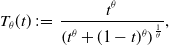 \begin{equation*}T_\theta(t)\,:\!=\,\frac{t^\theta}{\left(t^\theta+(1-t)^\theta\right)^{\frac{1}{\theta}}},\end{equation*}
where $\theta \in [0.3,0.8]$
. Additionally, we consider three cases for the distribution of the random loss X.
$\theta \in [0.3,0.8]$
. Additionally, we consider three cases for the distribution of the random loss X.
We first assume that the random loss X follows a uniform distribution with CDF given by
 \begin{equation*}F_X(x)=\frac{x}{M}, \quad \forall x \in [0,M] \quad \text{and}\quad M = 10.\end{equation*}
Figure 1(a) plots the distortion functions $T_\theta$
for different values of
$T_\theta$
for different values of $\theta$
. The figure shows that as
$\theta$
. The figure shows that as $\theta$
increases,
$\theta$
increases, $T_\theta$
approaches the identity function, and the intersection point
$T_\theta$
approaches the identity function, and the intersection point $t_1$
shifts to larger values. Moreover, functions with smaller values of
$t_1$
shifts to larger values. Moreover, functions with smaller values of $\theta$
are more concave near 0 and more convex near 1, implying that the policyholder places greater emphasis on extreme losses.
$\theta$
are more concave near 0 and more convex near 1, implying that the policyholder places greater emphasis on extreme losses.
The case where X follows a uniform distribution.

Figure 1. Long description
The image contains two line graphs. The first graph on the left shows the policyholder’s distortion function with three different theta values: 0.3, 0.5, and 0.7. The x-axis represents time (t) ranging from 0 to 1, and the y-axis represents the distortion function (Tb(t)) ranging from 0 to 1. The blue line represents theta equals 0.3, the red line represents theta equals 0.5, and the green line represents theta equals 0.7. A dashed black line is also present, indicating a reference or baseline. The second graph on the right shows the insurer’s expected profit under SE, with the x-axis representing t1 ranging from 0.15 to 0.4 and the y-axis representing the expected profit (VIn) ranging from 0.08 to 0.2. The red line in this graph shows a peak around t1 equals 0.3. The graphs illustrate the relationship between the policyholder’s distortion function and the insurer’s expected profit under different conditions.
Figure 1(b) depicts the insurer’s expected profit under the Stackelberg optimal contract as a function of $t_1$
. The result shows that the insurer’s expected profit does not vary monotonically with
$t_1$
. The result shows that the insurer’s expected profit does not vary monotonically with $\theta$
or the intersection point
$\theta$
or the intersection point $t_1$
. Notably, it reaches a maximum around
$t_1$
. Notably, it reaches a maximum around $t_1 \approx 0.32$
.
$t_1 \approx 0.32$
.
Alternatively, assume now that the loss random variable X follows a truncated exponential distribution, with CDF given by
 \begin{equation*}F_X(x) = \frac{1 - \exp(-\lambda x)}{1 - \exp(-\lambda M)}, \quad \forall x \in [0, M], \ M=10, \quad \text{and}\quad \lambda \gt 0.\end{equation*}
Figure 2(a) plots the CDF for different values of $\lambda$
. It shows that as
$\lambda$
. It shows that as $\lambda$
increases, the CDF becomes steeper for small losses, implying that losses are more likely to take smaller values. Figure 2(b) plots the insurer’s profit as a function of
$\lambda$
increases, the CDF becomes steeper for small losses, implying that losses are more likely to take smaller values. Figure 2(b) plots the insurer’s profit as a function of $t_1$
for different values of
$t_1$
for different values of $\lambda$
. The insurer’s profit does not vary monotonically with the parameter
$\lambda$
. The insurer’s profit does not vary monotonically with the parameter $\theta$
or the intersection point
$\theta$
or the intersection point $t_1$
.
$t_1$
.
The case where X follows a truncated exponential distribution.

Figure 2. Long description
The image contains two line graphs. The left graph shows the cumulative distribution function for different values of lambda (0.1, 0.5, and 1) plotted against x. The right graph illustrates the insurer’s expected profit under SE for the same lambda values plotted against t1. Each graph has distinct curves representing different lambda values, with the left graph showing how the distribution function changes with x and the right graph showing how expected profit varies with t1. The curves indicate different behaviors based on the lambda values, with higher lambda values generally showing steeper changes.
The result also depends on the loss distribution parameter $\lambda$
. In particular, the insurer’s profit reaches its maximum around
$\lambda$
. In particular, the insurer’s profit reaches its maximum around $t_1 \approx 0.3$
when
$t_1 \approx 0.3$
when $\lambda = 0.1$
. When
$\lambda = 0.1$
. When $\lambda$
increases to
$\lambda$
increases to $0.5$
, meaning that the distribution becomes more concentrated on the left, the maximum shifts to about
$0.5$
, meaning that the distribution becomes more concentrated on the left, the maximum shifts to about $t_1 \approx 0.22$
, indicating that if the policyholder faces a lower probability of large losses, greater concern for extreme losses becomes more valuable to the insurer. When
$t_1 \approx 0.22$
, indicating that if the policyholder faces a lower probability of large losses, greater concern for extreme losses becomes more valuable to the insurer. When $\lambda$
increases further to 1, implying that losses are even more likely to be small, the maximum shifts slightly further left, and the insurer’s profit then decreases monotonically with
$\lambda$
increases further to 1, implying that losses are even more likely to be small, the maximum shifts slightly further left, and the insurer’s profit then decreases monotonically with $t_1$
. This suggests that the insurer achieves the highest profit when the policyholder places more weight on extreme loss events.
$t_1$
. This suggests that the insurer achieves the highest profit when the policyholder places more weight on extreme loss events.
Finally, assume that the random loss X follows a Kumaraswamy distribution with CDF given by
 \begin{equation*}F_X(x) = 1 - \big(1 - (\tfrac{x}{M})^a\big)^b, \quad \forall x \in [0, M], \ M=10, \quad \text{and}\quad a,b\gt 0.\end{equation*}
Figure 3(a) plots the CDFs for different combinations of a and b. The blue curve lies close to, but slightly below, the identity function, indicating that more losses are concentrated on the right compared to the uniform distribution. The red curve is more concave than the blue one, implying that larger losses are more likely. The green curve represents the most extreme right-skewed case among the three.
The case where X follows a Kumaraswamy distribution.

Figure 3. Long description
The image contains two line graphs. The left graph shows the cumulative distribution function for different parameter values. The x-axis represents the variable x, and the y-axis represents the cumulative distribution function F subscript X of x. Three lines are plotted: a blue line for parameters a equals 1.5 and b equals 1, a red line for parameters a equals 1.5 and b equals 0.5, and a green line for parameters a equals 2 and b equals 0.3. The right graph shows the insurer’s expected profit under SE for different parameter values. The x-axis represents t subscript 1, and the y-axis represents V superscript ln of I subscript g asterisk g asterisk. Three lines are plotted: a blue line for parameters a equals 1.5 and b equals 1, a red line for parameters a equals 1.5 and b equals 0.5, and a green line for parameters a equals 2 and b equals 0.3. The graphs illustrate how the cumulative distribution function and the insurer’s expected profit vary with different parameter values.
Figure 3(b) shows the corresponding insurer’s profit under these three scenarios. When $a = 1.5$
and
$a = 1.5$
and $b = 1$
, the insurer’s profit does not vary monotonically with
$b = 1$
, the insurer’s profit does not vary monotonically with $t_1$
, and it reaches its maximum around
$t_1$
, and it reaches its maximum around $t_1 \approx 0.32$
. When
$t_1 \approx 0.32$
. When $a = 1.5$
and
$a = 1.5$
and $b = 0.5$
, meaning the loss distribution becomes riskier in the sense of first-order stochastic dominance, the insurer’s profit decreases for all
$b = 0.5$
, meaning the loss distribution becomes riskier in the sense of first-order stochastic dominance, the insurer’s profit decreases for all $t_1$
. This suggests that when the underlying risk increases, the insurer’s profit declines regardless of the policyholder’s risk attitude. Moreover, the maximum shifts to the right, reaching about
$t_1$
. This suggests that when the underlying risk increases, the insurer’s profit declines regardless of the policyholder’s risk attitude. Moreover, the maximum shifts to the right, reaching about $t_1 \approx 0.37$
. When the loss becomes even riskier with
$t_1 \approx 0.37$
. When the loss becomes even riskier with $a = 2$
and
$a = 2$
and $b = 0.3$
, a similar decreasing pattern is observed, with the maximum shifting further to the right to approximately
$b = 0.3$
, a similar decreasing pattern is observed, with the maximum shifting further to the right to approximately $t_1 \approx 0.4$
.
$t_1 \approx 0.4$
.
6. Conclusion
In this paper, we study Stackelberg equilibria (Bowley optima) in a monopolistic centralized sequential-move insurance market. We consider a risk-neutral, profit-maximizing insurer who sets premia using a distortion premium principle, and a single policyholder who seeks to minimize a DRM.
We characterize Stackelberg equilibria explicitly, and we show that, in equilibrium, the optimal indemnity function exhibits a layer-type structure, providing full insurance over any loss layer on which the policyholder is more pessimistic than the insurer’s pricing functional about tail losses. Equilibrium contracts provide no coverage over loss layers on which the policyholder is less pessimistic than the insurer’s pricing functional about tail losses. When the policyholder and the insurer’s pricing functional are equally pessimistic about tail losses, the marginal indemnity may take an arbitrary shape, within the global feasibility constraints. Additionally, in equilibrium, the optimal pricing distortion function is determined by the policyholder’s degree of (weak) risk aversion, that is, whether the policyholder’s distortion function is above or below the identity function, such that prices never exceed the policyholder’s marginal willingness to insure tail losses.
When the policyholder is either weakly risk averse (with a distortion function that lies above the identity function) or strongly risk averse (with a concave distortion function), we show that the optimal contract provides full insurance, and the optimal pricing distortion function coincides with that of the policyholder. For policyholders who evaluate risk using a VaR risk measure at a confidence level $\alpha \in (0,1)$
, the optimal coverage includes an upper limit by providing full insurance for losses below the
$\alpha \in (0,1)$
, the optimal coverage includes an upper limit by providing full insurance for losses below the $\alpha$
-quantile while leaving the upper tail uninsured. For a policyholder who displays strong sensitivity to extreme losses, captured by an inverse-S-shaped distortion function, the optimal indemnity function takes the form of a deductible contract, whereby extreme losses are fully transferred to the insurer. Furthermore, we show that in an SE, both the insurance coverage and the insurer’s expected profit increase with the policyholder’s degree of strong or weak risk aversion. A more risk-averse policyholder will receive greater insurance coverage under an equilibrium optimal contract and is more valuable to the insurer.
$\alpha$
-quantile while leaving the upper tail uninsured. For a policyholder who displays strong sensitivity to extreme losses, captured by an inverse-S-shaped distortion function, the optimal indemnity function takes the form of a deductible contract, whereby extreme losses are fully transferred to the insurer. Furthermore, we show that in an SE, both the insurance coverage and the insurer’s expected profit increase with the policyholder’s degree of strong or weak risk aversion. A more risk-averse policyholder will receive greater insurance coverage under an equilibrium optimal contract and is more valuable to the insurer.
Moreover, we examine the Pareto efficiency of equilibrium contracts. Echoing recent work in the literature, we show that equilibrium contracts are Pareto optimal, but they do not induce a welfare gain to the policyholder, which is unsurprising in a monopoly. Conversely, any Pareto-optimal contract that leaves no welfare gain to the policyholder can be obtained as an SE contract.
Acknowledgments
We are grateful to two anonymous reviewers for comments. Mario Ghossoub acknowledges financial support from the Natural Sciences and Engineering Research Council of Canada (NSERC Grant No. 2024-03744). Bin Li acknowledges financial support from NSERC Grant No. 2020-04338. Benxuan Shi acknowledges financial support from the Society of Actuaries through the Hickman Scholars Program.
Appendix A. Proofs of main results
A.1. Proof of Lemma 3.4
For a given pricing distortion function g, assume that $q_g$
is optimal for (9), and we aim to show that
$q_g$
is optimal for (9), and we aim to show that $I_g(x)= x - q_g \left(F_X(x)\right)$
is optimal for (6). Consider any feasible solution I to (6), and let q(t) be the quantile function of the associated retention R(X), for all
$I_g(x)= x - q_g \left(F_X(x)\right)$
is optimal for (6). Consider any feasible solution I to (6), and let q(t) be the quantile function of the associated retention R(X), for all $t \in [0,1]$
. We saw in (8) that
$t \in [0,1]$
. We saw in (8) that
 \begin{align*}\rho^{Pol}(I,g)&=\rho^{Pol} (R(X)) + \Pi_g (I(X)) \\&=\int_0^1 q^{\prime}(t) \, \left[T(1-t) - g(1-t)\right]\,\mathrm{d}t + \int_0^1 \left(F_{X}^{-1}\right)^{\prime}(t) \, g(1-t)\,\mathrm{d}t.\end{align*}
Since $q_g$
is optimal for the problem given in (9), then the following inequality holds:
$q_g$
is optimal for the problem given in (9), then the following inequality holds:
 \begin{align*}\rho^{Pol}(I,g)&\geq \int_0^1 q_g^{\prime}(t) \, \left[T(1-t) - g(1-t)\right]\,\mathrm{d}t + \int_0^1 \left(F_{X}^{-1}\right)^{\prime}(t) \, g(1-t)\,\mathrm{d}t,\end{align*}
where, by Remark 3.3,
 \begin{equation*}q_g(t) = F_X^{-1}(t) - F^{-1}_{I_g(X)}(t), \ \forall t \in [0,1].\end{equation*}
Hence,
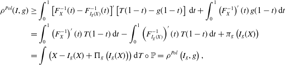 \begin{align*}\rho^{Pol}(I,g)&\geq \int_0^1 \big[ F_X^{-1}(t)-F^{-1}_{I_g(X)}(t) \big]^{\prime}\left[T(1-t) - g(1-t)\right]\,\mathrm{d}t + \int_0^1 \left(F_{X}^{-1}\right)^{\prime}(t) \, g(1-t)\,\mathrm{d}t \\&=\int_0^1\left(F_X^{-1}\right)^{\prime}(t)\,T(1-t)\,\mathrm{d}t-\int_0^1\left(F^{-1}_{I_g(X)}\right)^{\prime}(t)\,T(1-t) \, \mathrm{d}t + \pi_g\left(I_g(X)\right)\\&=\int \left(X-I_g(X)+\Pi_g\left(I_g(X)\right)\right)\mathrm{d}T\circ\mathbb{P}=\rho^{Pol}\left(I_g,g\right),\end{align*}
which implies that the indemnity function $I_g(x) = x - q_g \big( F_X (x) \big)$
is optimal for the policyholder’s problem (6).
$I_g(x) = x - q_g \big( F_X (x) \big)$
is optimal for the policyholder’s problem (6).
Conversely, we assume that the indemnity function $I_g$
, given by
$I_g$
, given by $I_g(x) = x - q_g \big( F_X (x) \big)$
is optimal for the policyholder’s problem (6), and we aim to show that the quantile
$I_g(x) = x - q_g \big( F_X (x) \big)$
is optimal for the policyholder’s problem (6), and we aim to show that the quantile $q_g$
is optimal for (9). Consider any feasible solution q to (9) and let
$q_g$
is optimal for (9). Consider any feasible solution q to (9) and let $I(x) = x - q(F_X(x))$
. We have that:
$I(x) = x - q(F_X(x))$
. We have that:
 \begin{align*}\rho^{Pol}\left(q,g\right)&=\int_0^1 q^{\prime}(t) \, \left[T(1-t) - g(1-t)\right]\,\mathrm{d}t + \int_0^1 \left(F_{X}^{-1}\right)^{\prime}(t) \, g(1-t)\,\mathrm{d}t \\&=\int\left(X- I(X) + \Pi_g\left(I(X)\right)\right) \,\mathrm{d}T\circ\mathbb{P}.\end{align*}
Since $I_g$
is optimal for (6), then the following inequality holds:
$I_g$
is optimal for (6), then the following inequality holds:
 \begin{align*}\rho^{Pol}(q,g)&\geq \int(X-I_g(X)+\Pi_g(I_g(X))) \,\mathrm{d}T\circ\mathbb{P}\\&= \int_0^1 q_g^{\prime}(t) \, [T(1-t) - g(1-t)]\,\mathrm{d}t + \int_0^1 \left(F_{X}^{-1}\right)^{\prime}(t) \, g(1-t)\,\mathrm{d}t=\rho^{Pol}( q_g,g),\end{align*}
which implies the optimality of $q_g$
for (9).
$q_g$
for (9).
A.2. Proof of Lemma 3.5
First, note that
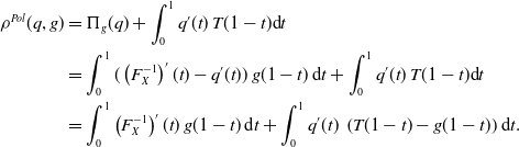 \begin{align*}\rho^{Pol}(q,g)&=\Pi_g(q)+\int_0^1q^{\prime}(t)\,T(1-t)\mathrm{d}t\\&=\int_0^1(\left(F_X^{-1}\right)^{\prime}(t)-q^{\prime}(t))\,g(1-t)\,\mathrm{d}t+\int_0^1q^{\prime}(t)\,T(1-t)\mathrm{d}t\\&=\int_0^1\left(F_X^{-1}\right)^{\prime}(t)\,g(1-t)\,\mathrm{d}t+\int_0^1q^{\prime}(t)\,\left(T(1-t)-g(1-t)\right)\mathrm{d}t.\end{align*}
The first term in the final line is independent of q, so minimizing the risk measure $\rho^{Pol}(q,g)$
over
$\rho^{Pol}(q,g)$
over $q\in\mathcal{Q}_L$
is equivalent to solving:
$q\in\mathcal{Q}_L$
is equivalent to solving:
 \begin{equation*}\min\limits_{q\in \mathcal{Q}_L}\int_0^1 q^{\prime}(t)\left(T(1-t)-g(1-t)\right)\,\mathrm{d}t.\end{equation*}
By the marginal indemnity function approach given in Assa (Reference Assa2015), the optimal quantile function $q_g$
must satisfy:
$q_g$
must satisfy:
 \begin{equation}\left(q_g\right)^{\prime}(t)=\left\{\begin{array}[c]{l@{\quad}l} 0, & g(1-t)\lt T(1-t), \\ \in[0,(F_X^{-1})^{\prime}(t)], & g(1-t)=T(1-t), \\ \left(F_X^{-1}\right)^{\prime}(t), & g(1-t)\gt T(1-t).\end{array}\right.\end{equation}
A.3. Proof of Theorem 3.9
First, note that the insurer’s profit can be expressed as:
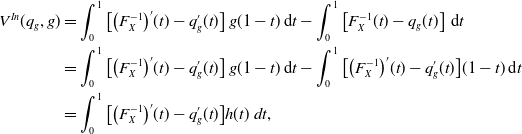 \begin{equation}\begin{split}V^{In}( q_{{g}},g)&=\int_0^1\big[\big(F_X^{-1}\big)^{\prime}(t)-q_{{g}}^{\prime}(t)\big]\,g(1-t)\,\mathrm{d}t-\int_{0}^1 \left[F_X^{-1}(t)-q_{{g}}(t)\right]\,\mathrm{d}t \\&=\int_0^1\big[\big(F_X^{-1}\big)^{\prime}(t)-q_{{g}}^{\prime}(t)\big]\,g(1-t)\,\mathrm{d}t-\int_{0}^1 \big[\big(F_X^{-1}\big)^{\prime}(t)-q_{{g}}^{\prime}(t)\big](1-t)\,\mathrm{d}t\\&= \int_0^1\big[\big(F_X^{-1}\big)^{\prime}(t)-q_{{g}}^{\prime}(t)\big] h(t) \ dt,\end{split}\end{equation}
where $h(t)\,:\!=\,t-1+g(1-t)$
, for all
$h(t)\,:\!=\,t-1+g(1-t)$
, for all $t \in [0,1]$
. Consider now the following three sets:
$t \in [0,1]$
. Consider now the following three sets:
 \begin{align*}\mathcal{A}_1 =\left\{t \in [0,1]\,:\, h(t) \lt t-\widetilde T(t)\right\},\quad \mathcal{A}_2 &=\left\{t\in [0,1]\,:\, h(t)=t- \widetilde T(t)\right\}, \quad \hbox{and} \quad \\ \mathcal{A}_3 &= \left\{t\in [0,1]\,:\, h(t)\gt t-\widetilde T(t)\right\}.\end{align*}
where $\widetilde T$
is the conjugate of the distortion function T. Then, it follows from Lemma 3.5 that
$\widetilde T$
is the conjugate of the distortion function T. Then, it follows from Lemma 3.5 that
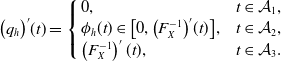 \begin{equation}\big( q_h \big)^{\prime}(t)=\left\{\begin{array}[c]{l@{\quad}l}0, &t\in\mathcal{A}_1,\\ \phi_{h}(t)\in\big[0,\big(F_X^{-1}\big)^{\prime}(t)\big], & t\in\mathcal{A}_2,\\ \left(F_X^{-1}\right)^{\prime}(t), &t\in\mathcal{A}_3.\end{array}\right.\end{equation}
The insurer’s profit in (A2) can then be rewritten as follows:
 \begin{align}V^{In}\left( q_{{h}},h\right)&= \int_{ 0}^1\left(F_X^{-1}\right)^{\prime}(t)\,h(t)\,\unicode{x1D7D9}_{\mathcal{A}_1}(t)\,\mathrm{d}t+\int_{0}^1\big[\big(F_X^{-1}\big)^{\prime}(t)-\phi_{h}(t)\big]\,h(t)\,\unicode{x1D7D9}_{\mathcal{A}_2}(t)\,\mathrm{d}t.\end{align}
Note that on $\mathcal{A}_2$
, the optimal retention function allows for some flexibility as long as
$\mathcal{A}_2$
, the optimal retention function allows for some flexibility as long as $q_h\in\mathcal{Q}_L$
. The arbitrary choice of
$q_h\in\mathcal{Q}_L$
. The arbitrary choice of $\phi_h(t)$
does not affect the policyholder’s risk exposure level, but it does impact the insurer’s profit. To maximize the insurer’s profit, we must take a further step to determine the value of
$\phi_h(t)$
does not affect the policyholder’s risk exposure level, but it does impact the insurer’s profit. To maximize the insurer’s profit, we must take a further step to determine the value of $\phi_h$
when
$\phi_h$
when $t \in \mathcal{A}_2$
. This is achieved by analyzing the profit over a finer partition
$t \in \mathcal{A}_2$
. This is achieved by analyzing the profit over a finer partition $\left\{\mathcal{B}_i\right\}_{i=1}^3$
such that:
$\left\{\mathcal{B}_i\right\}_{i=1}^3$
such that:
 \begin{equation*}\mathcal{B}_1=\{t \in [0,1]\,: \, \widetilde T(t)\lt t\}, \ \ \mathcal{B}_2=\{t \in [0,1]: \ \widetilde T(t)=t\}, \ \ \hbox{and} \ \ \mathcal{B}_3=\{t \in [0,1]\,:\, \widetilde T(t)\gt t\}.\end{equation*}
The insurer’s profit in (A4) becomes:
 \begin{align}V^{In}\left( q_{{h}},h\right) &=\int_0^1\left(F_X^{-1}\right)^{\prime}(t)\,h(t)\,\unicode{x1D7D9}_{\mathcal{A}_1}(t)\,\mathrm{d}t+\sum_{i=1}^3 \int_0^1\left[\left(F_X^{-1}\right)^{\prime}(t)-\phi_{h}(t)\right]h(t)\,\unicode{x1D7D9}_{\mathcal{A}_2}(t) \cdot \unicode{x1D7D9}_{\mathcal{B}_i}(t ) \ \mathrm{d}t \nonumber \\&= \int_0^1\left(F_X^{-1}\right)^{\prime}(t)\,h(t)\,\unicode{x1D7D9}_{\mathcal{A}_1}(t)\,\mathrm{d}t+\sum_{i=1}^3 \int_0^1\left[\left(F_X^{-1}\right)^{\prime}(t)-\phi_{h}(t)\right]h(t)\,\unicode{x1D7D9}_{\mathcal{A}_2\cap \mathcal{B}_i}(t) \ \mathrm{d}t.\end{align}
We consider the following three cases:
-
(1) On
$\mathcal{A}_2 \cap \mathcal{B}_1$
,
$h(t)=t-\widetilde T(t)\gt 0$
. Thus, the insurer’s profit in (A5) is decreasing in
$\phi_h(t)$
, and it is optimal to set
$\phi_{h}(t)=0$
. -
(2) On
$\mathcal{A}_2 \cap \mathcal{B}_2$
,
$h(t)=t-\widetilde T(t) = 0$
. The profit contribution is always zero regardless of the value of
$\phi_{h} (t)$
. Thus,
$\phi_{h} (t)$
can take any value in
$\left[0,\left(F_X^{-1}\right)^{\prime}(t)\right]$
without affecting the insurer’s profit. -
(3) On
$\mathcal{A}_2 \cap \mathcal{B}_3$
,
$h(t)=t-\widetilde T(t)\lt 0$
. The insurer’s profit is increasing in
$\phi_h(t)$
. Thus, it is optimal to set
$\phi_{h}(t)=\left(F_X^{-1}\right)^{\prime}(t)$
.









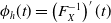
Hence, for a given h, the marginal quantile of the optimal retention can be written as:
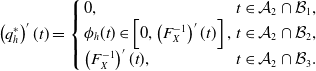 \begin{equation}\left(q^*_{h}\right)^{\prime}(t)=\left\{\begin{array}[c]{ll} 0, &t\in \mathcal{A}_2\cap\mathcal{B}_1, \\ \phi_{h}(t)\in\left[0,\left(F_X^{-1}\right)^{\prime}(t)\right], & t\in\mathcal{A}_2\cap\mathcal{B}_2, \\ \left(F_X^{-1}\right)^{\prime}(t), &t\in \mathcal{A}_2\cap\mathcal{B}_3. \end{array}\right.\end{equation}
It then follows from (A3) and (A6) that:
 \begin{equation}\left(q^*_{h}\right)^{\prime}(t)=\left\{\begin{array}[c]{ll}0, &t\in\mathcal{A}_1 \cup \left(\mathcal{A}_2 \cap \mathcal{B}_1\right), \\ \phi_{h}(t)\in\left[0,\left(F_X^{-1}\right)^{\prime}(t)\right], & t\in\mathcal{A}_2 \cap\mathcal{B}_2, \\ \left(F_X^{-1}\right)^{\prime}(t), &t\in\mathcal{A}_3\cup\left(\mathcal{A}_2 \cap\mathcal{B}_3\right). \end{array}\right.\end{equation}
Using (A7) and the fact that $h(t) =0$
on
$h(t) =0$
on $\mathcal{A}_2 \cap \mathcal{B}_2$
, the insurer’s profit in (A5) reduces to:
$\mathcal{A}_2 \cap \mathcal{B}_2$
, the insurer’s profit in (A5) reduces to:
 \begin{align*}V^{In}\left( q^*_{h},h\right)&= \int_0^1 (F_X^{-1})'(t)\,h(t)\bigl[ \unicode{x1D7D9} _{\mathcal{A}_1}(t) + \unicode{x1D7D9}_{\mathcal A_2\cap\mathcal B_1}(t)\bigr]\ \mathrm{d}t \\&=\int_0^1\left(F_X^{-1}\right)^{\prime}(t)\, h(t) \ \unicode{x1D7D9}_{\mathcal{A}_1\cup ( \mathcal{A}_2\cap \mathcal{B}_1 )}(t) \ \mathrm{d}t , \ \text{since $\mathcal{A}_1$ and $\mathcal{A}_2$ are disjoint.}\end{align*}
Moreover,
 \begin{align*}\mathcal{A}_1 \cup \big( \mathcal{A}_2 \cap \mathcal{B}_1 \big)&= \big( \mathcal{A}_1 \cup \mathcal{A}_2 \big) \ \cap \ \big( \mathcal{A}_1 \cup \mathcal{B}_1\big).\end{align*}
Since $\{\mathcal{B}_i\}_{i=1}^3$
forms a partition of [0,1], we have:
$\{\mathcal{B}_i\}_{i=1}^3$
forms a partition of [0,1], we have:
 \begin{equation*}\mathcal A_1 \cup\mathcal B_1=\mathcal B_1 \cup \left(\mathcal A_1 \cap(\mathcal B_2\cup\mathcal B_3)\right).\end{equation*}
Combining the above identities yields:
 \begin{equation*}\mathcal{A}_1\cup(\mathcal{A}_2\cap\mathcal{B}_1)=\left[(\mathcal{A}_1 \cup \mathcal{A}_2) \cap\mathcal{B}_1\right]\cup\left[\mathcal{A}_1 \cap ( \mathcal{B}_2 \cup \mathcal{B}_3)\right],\end{equation*}
which is a union of disjoint sets. Therefore,
 \begin{equation*}V^{In}(q_h^*,h)=\int_0^1 (F_X^{-1})'(t)\,h(t)\left[\mathbf 1_{(\mathcal{A}_1 \cup \mathcal{A}_2) \cap \mathcal{B}_1}(t)+\mathbf 1_{\mathcal{A}_1 \cap (\mathcal{B}_2 \cup \mathcal{B}_3)}(t)\right] \ \mathrm{d}t.\end{equation*}
The insurer’s optimization problem given in (12) thus reduces to the following:
 \begin{align}\max\limits_{h} \ \left\{\int_0^1\left(F_X^{-1}\right)^{\prime}(t)\, h(t)\left[ \unicode{x1D7D9}_{\{h(t)\leq t-\widetilde T(t)\}}\unicode{x1D7D9}_{\{\widetilde T(t)\lt t\}}+\unicode{x1D7D9}_{\{h(t)\lt t-\widetilde T(t)\}}\unicode{x1D7D9}_{\{\widetilde T(t)\geq t\}}\right]\mathrm{d}t\right\}.\end{align}
Since the integrand depends on h only through the pointwise value h(t), the above problem (A8) can be solved by maximizing the integrand pointwise. Fix $t_0\in(0,1)$
and consider the auxiliary maximization problem:
$t_0\in(0,1)$
and consider the auxiliary maximization problem:
 \begin{equation*}\max_{y\geq 0} \ m(y;\,t_0),\end{equation*}
where the auxiliary function $m(y; t_0)$
is given by
$m(y; t_0)$
is given by
 \begin{equation*}m(y;\,t_0)\,:\!=\, y \left[ \unicode{x1D7D9}_{\{y\leq t_0-\widetilde T(t_0)\}}\unicode{x1D7D9}_{\{ \widetilde T(t_0)\lt t_0\}} + \unicode{x1D7D9}_{\{y\lt t_0-\widetilde T(t_0)\}} \unicode{x1D7D9}_{\{ \widetilde T(t_0) \geq t_0\}}\right].\end{equation*}
For a fixed $t_0$
, the function
$t_0$
, the function $m(y; t_0)$
is piecewise linear in y. Let
$m(y; t_0)$
is piecewise linear in y. Let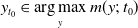 $y_{t_0}\in\underset{y}{\arg\max}\, m(y;\,t_0)$
. The maximum value of
$y_{t_0}\in\underset{y}{\arg\max}\, m(y;\,t_0)$
. The maximum value of $m(y;\,t_0)$
is given by
$m(y;\,t_0)$
is given by
 \begin{equation*}m(y_{t_0};\,t_0)=\left\{\begin{array}[c]{l@{\quad}l} t_0-\widetilde T(t_0), &\widetilde T(t_0)\lt t_0, \\0,& \widetilde T(t_0)\geq t_0,\end{array}\right.\end{equation*}
and any maximizer $y_{t_0}$
satisfies:
$y_{t_0}$
satisfies:
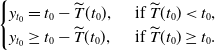 \begin{equation}\begin{cases}y_{t_0} = t_0-\widetilde T(t_0), \ & \text{ if $\widetilde T(t_0)\lt t_0$}, \\y_{t_0} \geq t_0-\widetilde T(t_0), \ & \text{ if $\widetilde T(t_0) \geq t_0$}.\end{cases}\end{equation}
for any $t_0\in (0,1)$
. We now proceed to the characterization of optimal solutions to (A8) through the following Lemma.
$t_0\in (0,1)$
. We now proceed to the characterization of optimal solutions to (A8) through the following Lemma.
Lemma A.1. A function $h^*$
is optimal to (A8) if and only if for every
$h^*$
is optimal to (A8) if and only if for every $t_0 \in (0,1)$
,
$t_0 \in (0,1)$
, $h^*(t_0)=y_{t_0}$
, where
$h^*(t_0)=y_{t_0}$
, where $y_{t_0}$
satisfies (A9).
$y_{t_0}$
satisfies (A9).
Proof. Assume that $h^*$
is a solution to (A8). We show that
$h^*$
is a solution to (A8). We show that $h^* (t_0)= y_{t_0}$
, where
$h^* (t_0)= y_{t_0}$
, where $y_{t_0}$
satisfies (A9). We consider the following two cases.
$y_{t_0}$
satisfies (A9). We consider the following two cases.
-
(1) If
$\widetilde T(t_0)\lt t_0,$
we aim to show that
$h^*(t_0)=t_0-\widetilde T(t_0)$
for any
$t_0\in(0,1)$
. Suppose for the sake of contradiction that
\begin{equation*}h^*(t_0)\neq t_0-\widetilde T(t_0).\end{equation*}
Since
$\widetilde T(t_0)\lt t_0$
and
$\widetilde T$
is continuous (being differentiable), we can find an arbitrary small
$\epsilon\gt 0$
such that
\begin{equation*}\widetilde T(t)\lt t, \ \ \text{when $t\in(t_0-\epsilon,t_0+\epsilon)$}.\end{equation*}
If
$h^*(t_0)\lt t_0-\widetilde T(t_0)$
, we have
$m(h^*(t_0);\,t_0)=h^*(t_0)$
. Then, there exists a function
$\widetilde h$
such that:
\begin{equation*}\widetilde h(t) =\begin{cases}y_{t}\gt h^*(t), & t\in(t_0-\epsilon,t_0+\epsilon), \\h^*(t), & t\notin(t_0-\epsilon,t_0+\epsilon),\end{cases}\end{equation*}
where
$y_t$
satisfies (A9), which implies the following:
\begin{align*}V^{In}\left( q^*_{\widetilde h},\widetilde h\right)-V^{In}\left( q^*_{h^*},h^*\right)&=\int_{t_0-\epsilon}^{t_0+\epsilon}\left(F_X^{-1}\right)^{\prime}(t)\, \left[m(y_{t}; \, t)- m\left(h^*(t);\,t\right) \right]\mathrm{d}t\\&= \int_{t_0-\epsilon}^{t_0+\epsilon}\left(F_X^{-1}\right)^{\prime}(t)\, \left[y_t- h^*(t)\right]\mathrm{d}t\gt 0,\end{align*}
since
$y_t\gt h^*(t)$
when
$t\in(t_0-\epsilon,t_0+\epsilon)$
. Hence, this contradicts the fact that
$h^*$
is optimal for problem (A8).If, in contrast,
$h^*(t_0)\gt {t_0}-\widetilde T(t_0)$
, then
$m\left(h^*(t_0);\,t_0\right)=0$
. With the same
$\epsilon$
, there exists a function
$\widetilde h$
such that:
\begin{equation*}\widetilde h(t)= \begin{cases}y_{t}\lt h^*(t) , & t\in(t_0-\epsilon,t_0+\epsilon), \\h^*(t), & t\notin(t_0-\epsilon,t_0+\epsilon).\end{cases}\end{equation*}
Hence,
\begin{align*}V^{In}\left( q^*_{\widetilde h},\widetilde h\right)-V^{In}\left( q^*_{h^*},h^*\right)&=\int_{t_0-\epsilon}^{t_0+\epsilon}\left(F_X^{-1}\right)^{\prime}(t)\, \left[m(y_{t}; \, t)- m\left(h^*(t);\,t\right)\right]\mathrm{d}t\\&= \int_{t_0-\epsilon}^{t_0+\epsilon}\left(F_X^{-1}\right)^{\prime}(t)\, \left(y_t- 0\right)\mathrm{d}t\gt 0,\end{align*}
which also contradicts the optimality of
$h^*$
for (A8). Therefore,
$h^*(t_0)=t_0-\widetilde T(t_0)$
, for any
$t_0\in(0,1)$
, when
$\widetilde T(t_0)\lt t_0$
. -
(2) If
$\widetilde T(t_0)\geq t_0,$
we aim to show that
$ h^*(t_0)\geq t_0-\widetilde T(t_0)$
, for any
$t_0 \in (0,1)$
. Suppose for the sake of contradiction that
\begin{equation*}h^*(t_0)\lt t_0-\widetilde T(t_0).\end{equation*}
Then,
\begin{equation*}m\left(h^*(t_0);\,t_0\right) = h^*(t_0)\lt t_0-\widetilde T(t_0) \leq 0.\end{equation*}
There exists an arbitrary small
$\epsilon \gt 0$
such that
$\widetilde T(t)\geq t$
on
$(t_0-\epsilon,t_0]$
or on
$[t_0,t_0+\epsilon)$
. First, assume that
$\widetilde T(t)\geq t$
on
$(t_0-\epsilon,t_0]$
. Then, there exists a function
$\widetilde h$
such that:
\begin{equation*}\widetilde h(t)=\begin{cases}y_{t}\gt h^*(t), & t\in(t_0-\epsilon,t_0], \\h^*(t), & t\notin(t_0-\epsilon,t_0].\end{cases}\end{equation*}
Therefore,
\begin{align*}V^{In}\left( q^*_{\widetilde h},\widetilde h\right)-V^{In}\left( q^*_{h^*},h^*\right)&=\int_{t_0-\epsilon}^{t_0}\left(F_X^{-1}\right)^{\prime}(t)\, \left[m(y_{t}; \, t)- m\left(h^*(t);\,t\right)\right]\mathrm{d}t\\&= \int_{t_0-\epsilon}^{t_0}\left(F_X^{-1}\right)^{\prime}(t)\, \left[0- m\left(h^*(t);\, t\right)\right]\mathrm{d}t\gt 0,\end{align*}
since
$m\left(h^*(t);\,t\right)\lt 0$
when
$t\in(t_0-\epsilon,t_0]$
, which leads to a contradiction. Hence,
\begin{equation*}h^*(t_0)\geq t_0-\widetilde T(t_0).\end{equation*}
Moreover, we can derive a similar result if
$\widetilde T(t)\geq t$
on
$[t_0,t_0+\epsilon)$
. In sum, for any
$t_0\in[0,1]$
, we obtain: (A10)
\begin{equation}\begin{cases}h^*(t_0)=t_0-\widetilde T(t_0), & \text{ if} \ \widetilde T(t_0)\lt t_0, \\h^*(t_0) \geq t_0-\widetilde T(t_0), & \text{ if} \ \widetilde T(t_0)\geq t_0. \end{cases}\end{equation}






































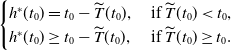
Conversely, assume that $h^*$
satisfies (A10). We show that
$h^*$
satisfies (A10). We show that $h^*$
is optimal for (A8). We first note that the insurer’s expected profit under
$h^*$
is optimal for (A8). We first note that the insurer’s expected profit under $(q^*_{h^*}, h^*)$
is given by
$(q^*_{h^*}, h^*)$
is given by
 \begin{equation*}V^{In}\left( q^*_{h^*},h^*\right) = \int_0^1\left(F_X^{-1}\right)^{\prime}(t)\,(t-\widetilde T(t))\unicode{x1D7D9}_{\{\widetilde T(t)\lt t\}} \, \mathrm{d}t.\end{equation*}
For any other feasible solution h, we compare the insurer’s expected profit under $h^*$
and h. Specifically, from the structure of (A8), we have
$h^*$
and h. Specifically, from the structure of (A8), we have
 \begin{align*}&V^{In}\left( q^*_{h^*},h^*\right)-V^{In}\left( q^*_{h},h\right) \\& \quad=\int_0^1\left(F_X^{-1}\right)^{\prime}(t)\,(t-\widetilde T(t))\unicode{x1D7D9}_{\{\widetilde T(t)lt t\}}\mathrm{d}t\\& \qquad -\int_0^1\left(F_X^{-1}\right)^{\prime}(t)\, h(t) \big[\unicode{x1D7D9}_{\{h(t)\leq t-\widetilde T(t)\}}\unicode{x1D7D9}_{\{\widetilde T(t)\lt t\}}(t)+\unicode{x1D7D9}_{\{h(t)\lt t-\widetilde T(t)\}}\unicode{x1D7D9}_{\{\widetilde T(t)= t\}}(t) +\unicode{x1D7D9}_{\{h(t)\lt t-\widetilde T(t)\}}\unicode{x1D7D9}_{\{\widetilde T(t)\gt t\}}(t)\big]\mathrm{d}t.\end{align*}
That is,
 \begin{align}V^{In}\left( q^*_{h^*},h^*\right)-V^{In}\left( q^*_{h},h\right)&=\int_0^1\left(F_X^{-1}\right)^{\prime}(t)\,\left[t-\widetilde T(t)-h(t)\unicode{x1D7D9}_{\{h(t)\leq t-\widetilde T(t))\}}\right]\unicode{x1D7D9}_{\{\widetilde T(t)\lt t\}}\mathrm{d}t\nonumber\\&\qquad-\int_0^1\left(F_X^{-1}\right)^{\prime}(t)\, h(t) \left[\unicode{x1D7D9}_{\{h(t)\lt t-\widetilde T(t)\}}\unicode{x1D7D9}_{\{\widetilde T(t)= t\}}+\unicode{x1D7D9}_{\{h(t)\lt t-\widetilde T(t)\}}\unicode{x1D7D9}_{\{\widetilde T(t)\gt t\}}\right]\mathrm{d}t.\end{align}
Looking at the first term of (A11), we know that
 \begin{align*}t-\widetilde T(t)-h(t)\unicode{x1D7D9}_{\{h(t)\leq t-\widetilde T(t)\}}&=\left\{\begin{array}[c]{l@{\quad}l}t-\widetilde T(t),& h(t)\gt t-\widetilde T(t) \\t-\widetilde T(t)-h(t),&h(t)\leq t-\widetilde T(t),\end{array}\right.\end{align*}
which is always nonnegative. For the second term,
 \begin{equation*}-h(t) \unicode{x1D7D9}_{\{h(t)\lt t-\widetilde T(t)\}} \ \begin{cases}=h(t) \unicode{x1D7D9}_{\{h(t)\lt 0\}}\geq 0, & \text{if }\widetilde T(t)=t,\\ \geq 0, & \text{if } \widetilde T(t)\gt t.\end{cases}\end{equation*}
Thus, both terms of (A11) are nonnegative, for all $t\in[0,1]$
, implying that the integrand is pointwise nonnegative. Therefore, the difference in profit is nonnegative, i.e.,
$t\in[0,1]$
, implying that the integrand is pointwise nonnegative. Therefore, the difference in profit is nonnegative, i.e.,
 \begin{equation*}V^{In}\left( q^*_{h^*},h^*\right)\geq V^{In}\left( q^*_{h},h\right).\end{equation*}
Hence, $h^*$
maximizes the insurer’s profit functional, thereby establishing sufficiency.
$h^*$
maximizes the insurer’s profit functional, thereby establishing sufficiency.
Moreover, when $h^*$
satisfies (A10), we can characterize the structure of the critical sets
$h^*$
satisfies (A10), we can characterize the structure of the critical sets $\mathcal{A}_1 \cup (\mathcal{A}_2 \cap \mathcal{B}_1)$
,
$\mathcal{A}_1 \cup (\mathcal{A}_2 \cap \mathcal{B}_1)$
, $\mathcal{A}_2 \cap \mathcal{B}_2$
, and
$\mathcal{A}_2 \cap \mathcal{B}_2$
, and $\mathcal{A}_3 \cup ( \mathcal{A}_2 \cap \mathcal{B}_3)$
that define
$\mathcal{A}_3 \cup ( \mathcal{A}_2 \cap \mathcal{B}_3)$
that define $q^*_{h^*}$
in (A7). First, if
$q^*_{h^*}$
in (A7). First, if $h^*$
satisfies (A10), we can clearly see that
$h^*$
satisfies (A10), we can clearly see that $\mathcal{A}_1 = \varnothing$
. Hence,
$\mathcal{A}_1 = \varnothing$
. Hence,
 \begin{equation*}\mathcal{A}_1 \cup \left(\mathcal{A}_2 \cap\mathcal{B}_1\right) =\{t \in [0,1]\,:\, t-\widetilde T(t)\gt 0\}.\end{equation*}
Moreover,
 \begin{equation*}\mathcal{A}_2\cap\mathcal{B}_2=\{t \in [0,1]\,:\, h^*(t)=t-\widetilde T(t)=0\},\end{equation*}
and
 \begin{align*}\mathcal{A}_3 \cup \left(\mathcal{A}_2 \cap\mathcal{B}_3\right)&= \{t \in [0,1]\,:\, h^*(t)\gt t-\widetilde T(t)\} \ \cup \ \{t\in [0,1]\,:\, h^*(t)=t-\widetilde T(t)\lt 0\}.\end{align*}
Additionally, since $\{ \mathcal{B}_i\}_{i=1}^3$
forms a partition over (0,1), it follows that
$\{ \mathcal{B}_i\}_{i=1}^3$
forms a partition over (0,1), it follows that
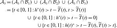 \begin{align*}\mathcal{A}_3&= (\mathcal{A}_3 \cap \mathcal{B}_1) \ \cup \ (\mathcal{A}_3 \cap \mathcal{B}_2) \ \cup \ (\mathcal{A}_3 \cap \mathcal{B}_3) \\&= \{t \in [0,1]\,:\, h^*(t) \gt t - \widetilde T(t), t \gt \widetilde T(t)\} \\&\qquad\qquad \cup \ \{ t\in [0,1]\,:\, h^*(t) \gt t- \widetilde T(t) =0\} \\&\qquad\qquad\qquad \cup \{t\in [0,1] \,:\, h(t)^* \gt t - \widetilde T(t), \widetilde T(t)\gt t\}.\end{align*}
The first intersection must be empty since $h^*$
satisfies (A10):
$h^*$
satisfies (A10):
 \begin{equation*}\mathcal{A}_3 \cap \mathcal{B}_1 = \varnothing.\end{equation*}
Hence, the union of $\mathcal{A}_3$
with
$\mathcal{A}_3$
with $\mathcal{A}_2 \cap \mathcal{B}_3$
reduces to the following:
$\mathcal{A}_2 \cap \mathcal{B}_3$
reduces to the following:
 \begin{equation*}\mathcal{A}_3 \cup \left(\mathcal{A}_2 \cap\mathcal{B}_3\right)=\{t\in [0,1]\,:\, h^*(t)\gt t-\widetilde T(t)=0\} \ \cup \ \{t\in [0,1]: \widetilde T(t)\gt t\}. \end{equation*}
Thus, the function $q^*_{h^*}$
given in (A7) can be written as follows:
$q^*_{h^*}$
given in (A7) can be written as follows:
 \begin{equation*}\left(q^*_{h^*}\right)^{\prime}(t)=\left\{\begin{array}[c]{l@{\quad}l} 0, &\widetilde T(t)\lt t, \\ \phi_{h}(t)\in\left[0,\left(F_X^{-1}\right)^{\prime}(t)\right], & t\in\{z; \ h^*(z)=z-\widetilde T(z)=0\}\\ \left(F_X^{-1}\right)^{\prime}(t), &t\in\{z; \ h^*(z)\gt z-\widetilde T(z)=0\} \cup \{ z; \ \widetilde T(z)\gt z \}.\ \end{array}\right.\end{equation*}
Since $\widetilde{g}^*(t)=t-h^*(t)$
, the optimal
$\widetilde{g}^*(t)=t-h^*(t)$
, the optimal $h^*$
leads to the following optimal pricing distortion function
$h^*$
leads to the following optimal pricing distortion function $\widetilde g^*$
:
$\widetilde g^*$
:
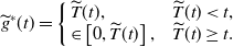 \begin{equation}\widetilde g^*(t)=\left\{\begin{array}[c]{l@{\quad}l} \widetilde T(t), &\widetilde T(t)\lt t, \\ \in\left[0,\widetilde T(t)\right], & \widetilde T(t)\geq t.\end{array}\right.\end{equation}
Consequently,
 \begin{equation*}\widetilde g^*(t)=\left\{\begin{array}[c]{l@{\quad}l}\widetilde T(t), &\widetilde T(t)\lt t,\\ \in\left[\,\sup \left\{z \lt t ; \ \widetilde g^*(z) \right\}, \widetilde T(t)\right], & \widetilde T(t)\geq t.\end{array}\right.\end{equation*}
We then obtain the optimal retention quantile $q^*$
as a function of the distortion premium function
$q^*$
as a function of the distortion premium function $g^*$
, as follows:
$g^*$
, as follows:
 \begin{equation*}\left(q^*_{{g}^*}\right)^{\prime}(t)=\left\{\begin{array}[c]{l@{\quad}l}0, &\widetilde T(t)\lt t, \\ \phi_{ g^*}(t)\in\big[0,\big(F_X^{-1}\big)^{\prime}(t)\big], & t\in\{z;\ \widetilde{g}^*(z)= \widetilde T(z)=z\}, \\ \left(F_X^{-1}\right)^{\prime}(t), &t\in\{z; \ \widetilde{g}^*(z)\lt \widetilde T(z)=z\}\cup\{z; \ \widetilde T(z)\gt z\} . \end{array}\right.\end{equation*}
A.4. Proof of Theorem 3.11
Consider two policyholders whose respective distortion functions $T_1$
and
$T_1$
and $T_2$
satisfy
$T_2$
satisfy $T_1(t) \leq T_2(t)$
for all
$T_1(t) \leq T_2(t)$
for all $t \in [0,1]$
. Then,
$t \in [0,1]$
. Then,
 \begin{equation*}T_1(\mathbb{P}[X \gt y]) \leq T_2(\mathbb{P}[X \gt y]), \quad \forall\, y \in [0,M].\end{equation*}
Let $(I_{g^*_1}^*, g_1^*)$
and
$(I_{g^*_1}^*, g_1^*)$
and $(I_{g^*_2}^*, g_2^*)$
denote the corresponding Stackelberg equilibria, where
$(I_{g^*_2}^*, g_2^*)$
denote the corresponding Stackelberg equilibria, where $\kappa_1^*$
and
$\kappa_1^*$
and $\kappa_2^*$
denote the marginal indemnity functions of the two policyholders, respectively, and satisfy Corollary 3.10. Hence, we obtain
$\kappa_2^*$
denote the marginal indemnity functions of the two policyholders, respectively, and satisfy Corollary 3.10. Hence, we obtain
 \begin{equation*}\kappa^*_1 (y) \leq \kappa^*_2(y), \quad \text{for almost every $y \in [0,M]$}.\end{equation*}
The above inequality gives
 \begin{equation*}I_{g^*_1}^*(x) \le I_{g^*_2}^*(x), \quad \forall x \in [0,M].\end{equation*}
The insurer’s expected profits for the two policyholders are given by:
 \begin{equation*}V^{In}(I_{g^*_1}^*, g_1^*)= \int_0^1 \big(F_X^{-1}\big)^{\prime}(t)\, [t - \widetilde{T}_1(t)]\, \unicode{x1D7D9}_{\{\widetilde{T}_1(t) \lt t\}}\, \mathrm{d}t\ \ \hbox{ and } \ V^{In}(I_{g^*_2}^*, g_2^*)= \int_0^1 \big(F_X^{-1}\big)^{\prime}(t)\, [t - \widetilde{T}_2(t)]\, \unicode{x1D7D9}_{\{\widetilde{T}_2(t) \lt t\}}\, \mathrm{d}t,\end{equation*}
where $\widetilde T_1$
and
$\widetilde T_1$
and $\widetilde T_2$
denote the conjugates of
$\widetilde T_2$
denote the conjugates of $T_1$
and
$T_1$
and $T_2$
, respectively. Since
$T_2$
, respectively. Since $T_1(t) \leq T_2(t)$
for all
$T_1(t) \leq T_2(t)$
for all $t \in [0,1]$
, it follows that
$t \in [0,1]$
, it follows that $\widetilde{T}_1 (t) \geq \widetilde{T}_2 (t)$
, for all
$\widetilde{T}_1 (t) \geq \widetilde{T}_2 (t)$
, for all $t \in [0,1]$
. Hence,
$t \in [0,1]$
. Hence,
 \begin{equation*}t - \widetilde{T}_1(t) \leq t - \widetilde{T}_2(t), \quad \forall t \in [0,1],\end{equation*}
and,
 \begin{equation*}\{\widetilde{T}_1(t) \lt t\} \subseteq \{\widetilde{T}_2(t) \lt t\}.\end{equation*}
Therefore,
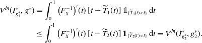 \begin{align*}V^{In}(I_{g^*_1}^*, g_1^*)&= \int_0^1 \big(F_X^{-1}\big)^{\prime}(t)\, [t - \widetilde{T}_1(t)]\, \unicode{x1D7D9}_{\{\widetilde{T}_1(t) \lt t\}}\, \mathrm{d}t\\&\leq \int_0^1 \big(F_X^{-1}\big)^{\prime}(t)\, [t - \widetilde{T}_2(t)]\, \unicode{x1D7D9}_{\{\widetilde{T}_2(t) \lt t\}}\, \mathrm{d}t=V^{In}(I_{g^*_2}^*, g_2^*).\end{align*}
Hence, the second policyholder is more profitable for the insurer than the first.
A.5. Proof of Proposition 4.1
Let $(I^*, \pi^*) \in \mathcal{I}_L \times \mathbb{R}$
be optimal for the problem given in (17) and assume for the sake of contradiction that
$(I^*, \pi^*) \in \mathcal{I}_L \times \mathbb{R}$
be optimal for the problem given in (17) and assume for the sake of contradiction that $(I^*, \pi^*)$
is not Pareto optimal. Then, there exists a contract
$(I^*, \pi^*)$
is not Pareto optimal. Then, there exists a contract $(I, \pi) \in \mathcal{I}_L \times \mathbb{R}$
such that
$(I, \pi) \in \mathcal{I}_L \times \mathbb{R}$
such that
 \begin{equation*}\rho^{{Pol}}(I, \pi) \leq \rho^{{Pol}}(I^*, \pi^*) \quad \text{and} \quad V^{{In}}(I, \pi) \geq V^{{In}}(I^*, \pi^*),\end{equation*}
with at least one strict inequality. Consequently,
 \begin{equation*}\rho^{{Pol}}(I, \pi) - V^{{In}}(I, \pi) \lt \rho^{{Pol}}(I^*, \pi^*) - V^{{In}}(I^*, \pi^*),\end{equation*}
which contradicts the optimality of $(I^*, \pi^*)$
for the problem given in (17). Hence, the contract
$(I^*, \pi^*)$
for the problem given in (17). Hence, the contract $(I^*, \pi^*)$
is Pareto optimal.
$(I^*, \pi^*)$
is Pareto optimal.
Conversely, suppose that the contract $(I^*, \pi^*)$
is Pareto optimal, and assume for the sake of contradiction that
$(I^*, \pi^*)$
is Pareto optimal, and assume for the sake of contradiction that $(I^*, \pi^*)$
is not optimal for (17). Then there exists a contract
$(I^*, \pi^*)$
is not optimal for (17). Then there exists a contract $(\widetilde{I}, \widetilde{\pi}) \in \mathcal{I}_L \times \mathbb{R}$
such that
$(\widetilde{I}, \widetilde{\pi}) \in \mathcal{I}_L \times \mathbb{R}$
such that
 \begin{equation*}\rho^{{Pol}}(\widetilde{I}, \widetilde{\pi}) - V^{{In}}(\widetilde{I}, \widetilde{\pi})\lt \rho^{{Pol}}(I^*, \pi^*) - V^{{In}}(I^*, \pi^*).\end{equation*}
Let $\hat{\pi} \,:\!=\, \widetilde{\pi} + \rho^{{Pol}}(I^*, \pi^*) - \rho^{{Pol}}(\widetilde{I}, \widetilde{\pi})$
. Then by translation invariance of
$\hat{\pi} \,:\!=\, \widetilde{\pi} + \rho^{{Pol}}(I^*, \pi^*) - \rho^{{Pol}}(\widetilde{I}, \widetilde{\pi})$
. Then by translation invariance of $\rho^{Pol}$
, we have:
$\rho^{Pol}$
, we have:
 \begin{equation*}\rho^{{Pol}}(\widetilde{I}, \hat{\pi}) = \rho^{{Pol}}(X - \widetilde{I}(X)) + \hat{\pi} = \rho^{{Pol}}(I^*, \pi^*).\end{equation*}
Moreover,
 \begin{align*}V^{{In}}(\widetilde{I}, \hat{\pi}) - V^{{In}}(I^*, \pi^*)&= \hat{\pi} - \mathbb{E}[\widetilde{I}(X)] - V^{{In}}(I^*, \pi^*) \\&= \left( \widetilde{\pi} + \rho^{{Pol}}(I^*, \pi^*) - \rho^{{Pol}}(\widetilde{I}, \widetilde{\pi}) \right) - \mathbb{E}[\widetilde{I}(X)] - V^{{In}}(I^*, \pi^*) \\&= \rho^{{Pol}}(I^*, \pi^*) - \rho^{{Pol}}(\widetilde{I}, \widetilde{\pi}) + V^{{In}}(\widetilde{I}, \widetilde{\pi}) - V^{{In}}(I^*, \pi^*)\gt 0.\end{align*}
Thus, the contract $(\widetilde{I}, \hat{\pi})$
satisfies
$(\widetilde{I}, \hat{\pi})$
satisfies
 \begin{equation*}\rho^{{Pol}}(\widetilde{I}, \hat{\pi}) = \rho^{{Pol}}(I^*, \pi^*) \quad \text{and} \quad V^{{In}}(\widetilde{I}, \hat{\pi}) \gt V^{{In}}(I^*, \pi^*),\end{equation*}
which contradicts the Pareto optimality of $(I^*, \pi^*)$
. Hence,
$(I^*, \pi^*)$
. Hence, $(I^*, \pi^*)$
is optimal for (17).
$(I^*, \pi^*)$
is optimal for (17).
A.6. Proof of Proposition 4.2
Consider a Stackelberg equilibrium $(I^*_{g^*}, g^*)$
inducing a contract
$(I^*_{g^*}, g^*)$
inducing a contract $(I^*_{g^*}, \pi^*_{g^*})$
, where
$(I^*_{g^*}, \pi^*_{g^*})$
, where $\pi^*_{g^*} \,:\!=\, \Pi_{g^*}(I^*_{g^*}(X)) = \int I^*_{g^*} \, d g^* \circ \mathbb{P}$
. By Proposition 4.1, to show that
$\pi^*_{g^*} \,:\!=\, \Pi_{g^*}(I^*_{g^*}(X)) = \int I^*_{g^*} \, d g^* \circ \mathbb{P}$
. By Proposition 4.1, to show that $(I^*_{g^*}, \pi^*_{g^*})$
is Pareto optimal, it suffices to show that it is optimal for Problem (17). By translation invariance of the distortion risk measure, a contract
$(I^*_{g^*}, \pi^*_{g^*})$
is Pareto optimal, it suffices to show that it is optimal for Problem (17). By translation invariance of the distortion risk measure, a contract $(I^*, \pi^*)$
is Pareto optimal if and only if the indemnity function
$(I^*, \pi^*)$
is Pareto optimal if and only if the indemnity function $I^*$
solves
$I^*$
solves
 \begin{equation*}\min_{I \in \mathcal{I}_L} \left\{ \rho^{{Pol}}(X - I(X)) + \mathbb{E}[I(X)] \right\}.\end{equation*}
Equivalently, using retention functions, the above problem becomes:
 \begin{equation*}\min_{R \in \mathcal{I}_L} \left\{ \rho^{{Pol}}(R(X)) + \mathbb{E}[X - R(X)] \right\}.\end{equation*}
Using $q(t) \,:\!=\, F_{R(X)}^{-1}(t)$
for a.e.
$q(t) \,:\!=\, F_{R(X)}^{-1}(t)$
for a.e. $t \in [0,1]$
, the above problem is equivalent to the following:
$t \in [0,1]$
, the above problem is equivalent to the following:
 \begin{align*}\min_{q \in \mathcal{Q}_L} \left\{ \int_0^1 q'(t)\left[ T(1 - t) - (1 - t) \right]\, \mathrm{d}t + \mathbb{E}[X] \right\}.\end{align*}
Since $(I^*_{g^*}, g^*)$
is a Stackelberg equilibrium, the optimal quantile
$(I^*_{g^*}, g^*)$
is a Stackelberg equilibrium, the optimal quantile $q^*_{g^*}$
characterized in Theorem 3.9 solves the above minimization problem. Hence, the induced contract
$q^*_{g^*}$
characterized in Theorem 3.9 solves the above minimization problem. Hence, the induced contract $(I^*_{g^*}, \pi^*_{g^*})$
is Pareto optimal. We now show that
$(I^*_{g^*}, \pi^*_{g^*})$
is Pareto optimal. We now show that $(I^*_{g^*}, \pi^*_{g^*})$
is individually rational but leaves the policyholder indifferent. First, note that the insurer’s expected profit under
$(I^*_{g^*}, \pi^*_{g^*})$
is individually rational but leaves the policyholder indifferent. First, note that the insurer’s expected profit under $(I^*_{g^*}, \pi^*_{g^*})$
satisfies
$(I^*_{g^*}, \pi^*_{g^*})$
satisfies
 \begin{align*}V^{In}(I^*_{g^*},\pi^*_{g^*})&=\int_0^1\left(F_X^{-1}\right)^{\prime}(t)\left[t-\widetilde T(t)\right]\,\unicode{x1D7D9}_{\{\widetilde T(t)\lt t\}}\,\mathrm{d}t\geq 0=V^{In}(0,0).\end{align*}
Moreover, for the policyholder, we have
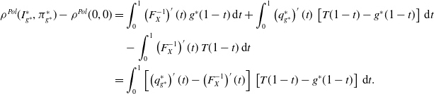 \begin{align*}\rho^{Pol}(I^*_{g^*},\pi^*_{g^*})-\rho^{Pol}(0,0)&=\int_0^1\left(F_X^{-1}\right)^{\prime}(t)\,g^*(1-t)\,\mathrm{d}t+\int_0^1\left(q^*_{g^*}\right)^{\prime}(t)\,\left[T(1-t)-g^*(1-t)\right] \, \mathrm{d}t\\&\quad-\int_0^1\left(F_X^{-1}\right)^{\prime}(t)\,T(1-t)\,\mathrm{d}t\\ &=\int_0^1\left[\left(q^*_{g^*}\right)^{\prime}(t)-\left(F_X^{-1}\right)^{\prime}(t)\right]\,\left[T(1-t)-g^*(1-t)\right] \, \mathrm{d}t.\end{align*}
Consider the following three cases:
-
(1) If
$\widetilde{T}(t) \lt t$
, then by optimality,
$\widetilde{g}^*(t) = \widetilde{T}(t)$
, or equivalently
$g^*(1 - t) = T(1 - t)$
. Hence,
$\left[\left(q^*_{g^*}\right)^{\prime}(t)-\left(F_X^{-1}\right)^{\prime}(t)\right]\,\left[T(1-t)-g^*(1-t)\right] =0$
. -
(2) If
$\widetilde{T}(t) = t$
and
$\widetilde{g}^*(t) \lt \widetilde{T}(t)$
, then
$\left(q^*_{g^*}\right)^{\prime}(t) = \left(F_X^{-1}\right)^{\prime}(t)$
. If
$\widetilde{T}(t) = t$
and
$\widetilde{g}^*(t) = \widetilde{T}(t)$
, then
$g^*(1 - t) = T(1 - t)$
. In both cases,
$\left[\left(q^*_{g^*}\right)^{\prime}(t)-\left(F_X^{-1}\right)^{\prime}(t)\right]\,\left[T(1-t)-g^*(1-t)\right] =0$
. -
(3) If
$\widetilde{T}(t) \gt t$
, then
$\left(q^*_{g^*}\right)^{\prime}(t) = \left(F_X^{-1}\right)^{\prime}(t)$
, and
$\left[\left(q^*_{g^*}\right)^{\prime}(t)-\left(F_X^{-1}\right)^{\prime}(t)\right]\,\left[T(1-t)-g^*(1-t)\right] =0$
.














Consequently, we finally obtain $\rho^{Pol}(I^*_{g^*},\pi^*_{g^*}) = \rho^{Pol}(0,0)$
.
$\rho^{Pol}(I^*_{g^*},\pi^*_{g^*}) = \rho^{Pol}(0,0)$
.
A.7. Proof of Proposition 4.3
Consider a Pareto optimal contract $(I^*, \pi^*)$
, such that
$(I^*, \pi^*)$
, such that $\rho^{Pol}(I^*,\pi^*) = \rho^{{Pol}}(0,0)$
. We show that this contract is induced by a Stackelberg equilibrium. First, note that under
$\rho^{Pol}(I^*,\pi^*) = \rho^{{Pol}}(0,0)$
. We show that this contract is induced by a Stackelberg equilibrium. First, note that under $(I^*, \pi^*)$
, the following holds by translation invariance and comonotonic additivity of
$(I^*, \pi^*)$
, the following holds by translation invariance and comonotonic additivity of $\rho^{Pol}$
:
$\rho^{Pol}$
:
 \begin{align*}\rho^{Pol}(I^*,\pi^*)&= \rho^{Pol}\left(X-I^*(X)\right) + \pi^*=\rho^{Pol}\left(X\right) - \rho^{Pol}\left(I^*(X)\right)+ \pi^*.\end{align*}
Since, $\rho^{Pol}(I^*,\pi^*) =\rho^{{Pol}}(0,0)=\rho^{{Pol}}(X)$
, we have that
$\rho^{Pol}(I^*,\pi^*) =\rho^{{Pol}}(0,0)=\rho^{{Pol}}(X)$
, we have that $\pi^* = \rho^{{Pol}}(I^*(X))$
. Moreover, since
$\pi^* = \rho^{{Pol}}(I^*(X))$
. Moreover, since $(I^*, \pi^*)$
is Pareto optimal, Proposition 4.1 implies that the quantile function
$(I^*, \pi^*)$
is Pareto optimal, Proposition 4.1 implies that the quantile function $q^*(t)\,:\!=\, F_X^{-1}(t) - F_{I^*(X)}^{-1}(t)$
satisfies
$q^*(t)\,:\!=\, F_X^{-1}(t) - F_{I^*(X)}^{-1}(t)$
satisfies
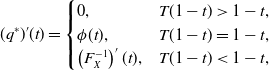 \begin{equation*}(q^*)'(t) =\begin{cases}0, & T(1 - t) \gt 1 - t, \\ \phi(t), & T(1 - t) = 1 - t, \\ \left(F_X^{-1}\right)'(t), & T(1 - t) \lt 1 - t,\end{cases}\end{equation*}
for some measurable function $\phi$
satisfying
$\phi$
satisfying $ \phi(t) \in[0,\left(F_X^{-1}\right)'(t)].$
Consider now the pair $(q^*, g^*_{I^*})$
, where the pricing distortion function
$(q^*, g^*_{I^*})$
, where the pricing distortion function $g^*_{I^*}$
coincides with the policyholder’s distortion function T. That is,
$g^*_{I^*}$
coincides with the policyholder’s distortion function T. That is,
 \begin{equation*}g^*_{I^*}(t) \,:\!=\, T(t), \quad \forall \, t \in [0, 1].\end{equation*}
Thus,
 \begin{equation*}\Pi_{g^*_{I^*}} \left( I^*(X) \right) = \int I^*(X)\, \mathrm{d}g^*_{I^*} \circ \mathbb{P}=\int I^*(X)\, \mathrm{d}T \circ \mathbb{P}= \rho^{{Pol}}(I^*(X))=\pi^*.\end{equation*}
Since $(q^*,g^*_{I^*})$
satisfies the optimality conditions of Theorem 3.9, it follows that
$(q^*,g^*_{I^*})$
satisfies the optimality conditions of Theorem 3.9, it follows that $(q^*,g^*_{I^*})$
solves the problem given in (12). Lemma 3.8 then implies that the market mechanism
$(q^*,g^*_{I^*})$
solves the problem given in (12). Lemma 3.8 then implies that the market mechanism $(I^*,g^*_{I^*})$
is a Stackelberg equilibrium. Hence, the Pareto optimal insurance contract
$(I^*,g^*_{I^*})$
is a Stackelberg equilibrium. Hence, the Pareto optimal insurance contract $(I^*,\pi^*)$
can be obtained from the Stackelberg equilibrium
$(I^*,\pi^*)$
can be obtained from the Stackelberg equilibrium $(I^*,g^*_{I^*})$
, where
$(I^*,g^*_{I^*})$
, where $\pi^* \,:\!=\, \Pi_{g^*_{I^*}} \left( I^*(X) \right)$
.
$\pi^* \,:\!=\, \Pi_{g^*_{I^*}} \left( I^*(X) \right)$
.




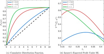


 Open access

