

1. INTRODUCTION
Over the last few decades, the Greenland ice sheet (GIS) has increasingly lost mass from 0.09 mm a−1 (1992–2001) to 0.59 mm a−1 (2002 to 2011) (e.g. Shepherd and others, Reference Shepherd2012; Vaughan and others, Reference Vaughan, Stocker, Qin, Plattner, Tignor, Allen, Boschung, Nauels, Xia, Bex and Midgley2013; Velicogna and others, Reference Velicogna, Sutterley and van den Broeke2014). Numerical models suggest that the cumulative mass loss from Greenland at the end of the 21st century could reach 27 cm of sea level equivalent (SLE) for the worse climate scenario (e.g. Church and others, Reference Church, Stocker, Qin, Plattner, Tignor, Allen, Boschung, Nauels, Xia, Bex and Midgley2013; Fettweis and others, Reference Fettweis2013; Yan and others, Reference Yan, Wang, Johannessen and Zhang2014; Fürst and others, Reference Fürst, Goelzer and Huybrechts2015). About half of the mass lost from Greenland today is due to surface melt, through runoff, while the other half results from solid ice discharge due to calving at the marine margins of the ice sheet (e.g. Rignot and Kanagaratnam, Reference Rignot and Kanagaratnam2006; van den Broeke and others, Reference van den Broeke2009). The relative importance of these two mechanisms varies among the different regions of Greenland. For example ice discharge is predominant in the Baffin Bay, Davis strait and Atlantic sectors, while the surface melt dominates in the Arctic, Labrador Sea and Greenland Sea sectors (e.g. van den Broeke and others, Reference van den Broeke2009; Sasgen and others, Reference Sasgen2012; Vaughan and others, Reference Vaughan, Stocker, Qin, Plattner, Tignor, Allen, Boschung, Nauels, Xia, Bex and Midgley2013).
The dynamical ice discharge is controlled by the acceleration of fast-flowing marine terminating outlet glaciers (e.g. Howat and others, Reference Howat, Joughin and Scambos2007; Nick and others, Reference Nick2013) triggered by different mechanisms, such as: decreased ice flow resistance due to glacier frontal retreat (e.g. Howat and others, Reference Howat, Joughin, Tulaczyk and Gogineni2005, Reference Howat, Joughin and Scambos2007), reduced basal and lateral drag (e.g. van der Veen and others, Reference van der Veen, Plummer and Stearns2011), increased melting at the ice/ocean interface (e.g. Holland and others, Reference Holland, Thomas, Young, Ribergaard and Lyberth2008; Murray and others, Reference Murray2010; Straneo and others, Reference Straneo2010), changes in basal lubrication (e.g. Zwally and others, Reference Zwally2002; Parizek and Alley, Reference Parizek and Alley2004; Sundal and others, Reference Sundal2011) and response to fast re-equilibration of calving-front geometry after calving events (e.g. Howat and others, Reference Howat, Joughin and Scambos2007). Because of the interplay among all these mechanisms (e.g. Vieli and Nick, Reference Vieli and Nick2011), these regions have been extensively monitored in order to improve present sea-level contribution estimates (e.g. Sohn and others, Reference Sohn, Jezek and van der Veen1998; Howat and others, Reference Howat, Joughin and Scambos2007; Holland and others, Reference Holland, Thomas, Young, Ribergaard and Lyberth2008; Joughin and others, Reference Joughin2008a, Reference Joughinb, Reference Joughinc; van der Veen and others, Reference van der Veen, Plummer and Stearns2011; Moon and others, Reference Moon, Joughin, Smith and Howat2012; Khan and others, Reference Khan2014; Münchow and others, Reference Münchow, Padman and Fricker2014; Mouginot and others, Reference Mouginot2015).
The Jakobshavn (JKB) glacier (West Greenland, Fig. 1d) is one of the major outlet glaciers since it drains ~7% of GIS ice mass (Csatho and others, Reference Csatho, Schenk, van der Veen and Krabill2008). It is also one of the outlet glaciers that has shown the largest retreat in recent decades. In fact, between 1995 and 2005 the ice velocities near the terminus of the glacier doubled and the glacier has been continuously thinning since the late 1990s (e.g. Sohn and others, Reference Sohn, Jezek and van der Veen1998; Holland and others, Reference Holland, Thomas, Young, Ribergaard and Lyberth2008; Joughin and others, Reference Joughin2008c; van der Veen and others, Reference van der Veen, Plummer and Stearns2011). Many mechanisms have been proposed to explain the behaviour of the JKB glacier, however ocean warming is considered as the most probable trigger for the recent frontal speed-ups.
(a) Observed Greenland topography (Bamber and others, Reference Bamber2013). (b) Simulated Greenland topography at the end of the spin-up run. (c) Differences between simulated topography at the end of the 24 ka spin-up and the observed topography. (d) Observed Greenland velocities (Joughin and others, Reference Joughin, Smith, Howat, Scambos and Moon2010). The red boxes show the locations of the five studied areas. (e) Simulated Greenland velocities at the end of the spin-up run. (f) Differences between simulated velocities at the end of the 24 ka spin-up and the observed velocities.

Similarly, on the eastern coast, the frontal ice velocities of Helheim (HLH) and Kangerdlugssuaq (KGL) glaciers increased from 2001 to 2006 (Joughin and others, Reference Joughin2008b). Ice velocities accelerated substantially in 2002 in relation to the HLH glacier and in 2005 for the KGL glacier, but slowed down after 2006 (e.g. Howat and others, Reference Howat, Joughin and Scambos2007; Murray and others, Reference Murray2010). Changes in sea surface temperature (Murray and others, Reference Murray2010), and the seismicity created by many large iceberg-calving episodes might be behind the variations in ice velocities (Joughin and others, Reference Joughin2008b). The different response timings of these glaciers has been related to the differences in the bedrock topography of the glaciers (Joughin and others, Reference Joughin2008b).
In contrast, the Petermann glacier (PTM) (North Greenland, Fig. 1d) was more stable than the others (e.g. Joughin and others, Reference Joughin, Smith, Howat, Scambos and Moon2010; Nick and others, Reference Nick2013) up to the end of the first decade of the 21st century, when two large calving events, in 2010 and 2012, led to a 33 km reduction in the length of its floating ice shelf and to ~15–30% increase in velocity compared with velocities observed before 2010 (Münchow and others, Reference Münchow, Padman and Fricker2014). Münchow and others (Reference Münchow, Padman and Fricker2014) relate these calving events to the formation of crevasses and to a thinning of the ice shelf, which weaken the structural integrity of the ice shelf.
In the north-eastern area of the GIS, three outlet glaciers, namely Nioghalvfjerdsfjorden Glacier (NG), Zachariae Isstrøm (ZI) and Storstrømmen Glacier (SG), drain the North East Greenland Ice Stream (NEGIS). The NEGIS is a unique glaciological feature in Greenland since this ice stream expands far inland, near the central dome of the ice sheet (Fahnestock and others, Reference Fahnestock, Abdalati, Joughin, Brozena and Gogineni2001). After a period of relative stability (1978–2003), the NEGIS has been affected by sustained dynamical changes probably caused by regional atmospheric and ocean warming (Khan and others, Reference Khan2014). While the ZI has exhibited an accelerated retreat, since 2012 the NG has retreated much more slowly in comparison, which Mouginot and others (Reference Mouginot2015) propose could be linked to the differences in their bed geometry. On the other hand, the SG is a surge glacier (a surge occurred between 1978 and 1984, Reeh and others, Reference Reeh, Mohr, Madsen, Oerter and Gundestrup2003), which explains the observed thickening of this glacier in the period 2003–12 (Khan and others, Reference Khan2014).
To investigate the mechanisms and processes behind present-day and future changes in the GIS and to reproduce the complex pattern of GIS ice velocities, numerical models of different spatial and physical complexities, spanning from single outlet glacier models (e.g. Nick and others, Reference Nick, van der Veen, Vieli and Benn2010, Reference Nick2013) to large-scale ice-sheet models (ISMs) (e.g. Price and others, Reference Price, Payne, Howat and Smith2011; Seddik and others, Reference Seddik, Greve, Zwinger, Gillet-Chaulet and Gagliardini2012; Goelzer and others, Reference Goelzer2013; Greve and Herzfeld, Reference Greve and Herzfeld2013), have been used to investigate the dynamics of the main fast-flowing areas. The studies based on these models suggest that the sea-level contribution of the GIS for the next century is dominated by surface mass balance (SMB) changes, while the outlet glacier dynamics only accounts for a small fraction of this contribution. These two processes are mutually competitive in removing mass from the GIS. For example, Goelzer and others (Reference Goelzer2013) show that the relative importance of outlet glacier dynamics in removing mass from the GIS decreases with decreasing SMB conditions. Using a three-dimensional (3-D) higher order model combined with a specific outlet glacier flow-line model, Goelzer and others (Reference Goelzer2013) estimate that outlet glacier dynamics will only account for 6–18% of the sea-level contribution by 2200 under a A1B SRES scenario (Nakićenović and others, Reference Nakićenović, Alcamo, Davis and de Vries2000). Price and others (Reference Price, Payne, Howat and Smith2011) use a 3-D higher-order ice flow model to which they apply a perturbation at the stress boundary condition at the marine termini of JKB, HLH and KGL outlet glaciers to evaluate their dynamical response. They estimate a total 21st century cumulative sea-level contribution from the GIS of ~46 mm SLE, with 13% coming from dynamical perturbations. Using an outlet glacier model, Nick and others (Reference Nick2013) calculate that ~80% of the sea-level contribution up to 2100 under the A1B SRES scenario (Nakićenović and others, Reference Nakićenović, Alcamo, Davis and de Vries2000) from PTM, KGL, JKB and HLH is likely to be due to dynamical changes, such as margin retreat or increased calving.
The mass conservation equation implies that the ice fluxes (in particular their divergence) together with surface and basal melting of the ice sheet determine the rate of change in the ice thickness (e.g. Greve and Blatter, Reference Greve and Blatter2009; Seroussi and others, Reference Seroussi2011). While SMB and outlet glacier basal melting can be computed independently from the ISMs, this is not the case for the dynamical changes resulting from ice thickness and calving variations. Therefore, an ISM is crucial to assess the variations in ice fluxes, especially for the fast-flowing areas, and, ultimately, ice volume variations (Seroussi and others, Reference Seroussi2011).
To model the dynamical changes in the fast flowing areas, high-resolution and higher-order numerical models could provide more accurate estimates than shallow ice approximation (SIA) and/or shallow shelf approximation (SSA) models. This is because the latter are not able to properly capture all the dynamical changes occurring at the ice-sheet margins due to the assumptions on which SIA relies (e.g. Seroussi and others, Reference Seroussi2011). However, Greve and Herzfeld (Reference Greve and Herzfeld2013) show that a SIA-only model, namely SICOPOLIS, with a high horizontal resolution of 5 km, satisfactorily reproduces the observed velocity fields in areas characterized by a complex topography and by fast-flowing conditions. Also, the hybrid SIA/SSA model GRISLI has been shown to perform very well in a GIS projection of sea-level contribution compared with full-Stokes models (Edwards and others, Reference Edwards2014). Compared with more comprehensive ISMs, the SIA and SIA/SSA-models suffer from various limitations and assumptions (see Section 4), however they are the only ISMs that have been coupled to climate models to date (e.g. Ganopolski and others, Reference Ganopolski, Calov and Claussen2010; Lipscomb and others, Reference Lipscomb2013). Further advantages of SIA and SIA/SSA models include: (1) the possibility to perform long-term simulations, which are required, for example, in determining the tipping point of the GIS. On the other hand, for more computationally demanding higher order models, this solution is still not feasible; (2) higher-order and full-Stokes models rely on SIA or hybrid models to spin-up the vertical ice temperature and ice velocities (e.g. Seddik and others, Reference Seddik, Greve, Zwinger, Gillet-Chaulet and Gagliardini2012) in order to benefit from a long-term initialization of the ice-sheet thermodynamics; (3) similarly to what is done with climate models, in order to assess the GIS response to ongoing and future climate change, it is important to keep a hierarchy of the physical complexities of ISMs (e.g. Blatter and others, Reference Blatter, Greve and Abe-Ouchi2011; Kirchner and others, Reference Kirchner, Hutter, Jakobsson and Gyllencreutz2011). This facilitates an objective perspective of the system.
The present work evaluates the link between the changes in SMB induced by the 20th and 21st century climate changes, the GIS geometrical evolution and the ice flux changes. We focus on the ice stream evolution of five of the main fast flowing areas in Greenland, namely PTM, NEGIS, KGL, HLH and JKB. We perform our simulations using the SIA/SSA ISM GRISLI (Ritz and others, Reference Ritz, Rommelaere and Dumas2001). Consequently, the present work also assesses the ability of a hybrid ISM to properly simulate observed and predicted changes in the GIS. We force GRISLI with the surface air temperatures and precipitations of the 20th and 21st centuries simulated by a set of seven atmosphere-ocean coupled general circulation models (AOGCMs) within the framework of the 5th phase of the Coupled Model Intercomparison Project (CMIP5, Taylor and others, Reference Taylor, Stouffer and Meehl2012) and with 20th century surface air temperature and precipitation from the regional atmospheric model MAR. The 21st century projections are based on the IPCC's Representative Concentration Pathways (RCP) 4.5 and 8.5 emissions scenarios (Moss and others, Reference Moss2010).
We now outline the main physical characteristics of the ISM GRISLI, and its initialization method as well as the climate forcing from the CMIP5 AOGCMs. We then analyze the results obtained with our simulations and discuss their implications with regard to the use of SIA/SSA ISMs and on the GIS ice flux evolution.
2. METHODS
2.1. The GRISLI ISM
The GRenoble Ice Shelf and Land Ice model (GRISLI, Ritz and others, Reference Ritz, Rommelaere and Dumas2001) is a 3-D thermo-mechanical ISM in which the dynamics of grounded ice is described by the SIA (Hutter, Reference Hutter1983) and fast ice streams and ice shelves are described by the SSA (MacAyeal, Reference MacAyeal1989). The grounding line is determined by a floatation criterion. The basal drag coefficient is inferred with an iterative inverse method based on the observed surface velocities (Edwards and others, Reference Edwards2014, and Supplementary Figure S1). The inverse method relies on the minimization of a cost function that measures the differences between observed and simulated velocities as a function of the basal drag β (e.g. Arthern and Gudmundsson, Reference Arthern and Gudmundsson2010; Morlighem and others, Reference Morlighem2010; Gillet-Chaulet and others, Reference Gillet-Chaulet2012).
GRISLI is run on a rectangular regular Cartesian grid at a 5 km × 5 km horizontal resolution using the polar stereographic projection with the standard parallel at 71°N and the central meridian at 39°W. In the vertical, GRISLI accounts for 21 layers of cold ice. The initial present-day bedrock elevation and ice-sheet thickness maps are derived from Bamber and others (Reference Bamber2013).
GRISLI is forced by monthly surface air temperature and total precipitation provided by the combination of MAR reference climatology and CMIP5 anomaly fields (further details in Section 2.3). To account for surface elevation changes during runtime, air surface temperature is corrected by an atmospheric uniform lapse rate (λ = 6.309 °C km−1, Fausto and others, Reference Fausto, Ahlstrøm, Van As, Bøggild and Johnsen2009). Changes in precipitation are related to changes in temperature by a precipitation correction factor (γ = 0.07, Quiquet and others, Reference Quiquet2012, and further details in Table 1), assuming that the saturation pressure of water vapour depends exponentially on the temperature (Charbit and others, Reference Charbit, Ritz and Ramstein2002).
Main characteristics and model parameters of GRISLI

The accumulation corresponds to the solid fraction of total precipitation, which is calculated using the empirical relationship introduced by Marsiat (Reference Marsiat1994). Ablation is computed using the positive degree-day (PDD) semi-empirical method by Reeh (Reference Reeh1991), which linearly relates the number of positive degree days to the amount of ice and snow melt through the degree-day factors (DDF) C snow and C ice. Both factors are derived from observations and vary spatially as a function of July temperature following Tarasov and Peltier (Reference Tarasov and Peltier2002). The main features of GRISLI are summarized in Table 1, and further details on the model physics can be found in Ritz and others (Reference Ritz, Rommelaere and Dumas2001).
2.2. Initialization of the ISM
Because of the slow diffusivity of surface temperature through the ice column and its influence on ice velocities, a spin-up is required to obtain realistic initial present-day vertical temperature conditions (Rogozhina and others, Reference Rogozhina, Martinec, Hagedoorn, Thomas and Fleming2011; Yan and others, Reference Yan, Zhang, Gao, Wang and Johannessen2013). We thus performed a long-term transient spin-up based on the index method (e.g. Cuffey and Marshall, Reference Cuffey and Marshall2000; Lhomme and others, Reference Lhomme, Clarke and Marshall2005; Greve and others, Reference Greve, Saito and Abe-Ouchi2011; Applegate and others, Reference Applegate, Kirchner, Stone, Keller and Greve2012; Quiquet and others, Reference Quiquet, Ritz, Punge and Salas y Mélia2013), according to the initialization protocol of the SeaRISE project (e.g. Greve and others, Reference Greve, Saito and Abe-Ouchi2011; Bindschadler and others, Reference Bindschadler2013; Nowicki and others, Reference Nowicki2013). To balance initialization-time and computational-time, the spin-up simulation covers the last 24 ka of the last glacial cycle, starting slightly before the Last Glacial Maximum (21 ka BP), similarly to Herzfeld and others (Reference Herzfeld2012). We performed a 125 ka spin-up for comparison. The temperature profiles obtained both inland (at GRIP site) and along the margins (at DYE3 site) are very similar to those obtained after 24 ka. We believe that the discrepancy between the two spin-ups does not significantly affect the conclusions of this work (Supplementary Figure S2). Finally, the ice-sheet topography is tuned by adding a correction term (Supplementary Table S1) to the melting factors C snow and C ice following Greve and others (Reference Greve, Saito and Abe-Ouchi2011).
At the end of the spin-up, compared with the observed ice topography (Bamber and others, Reference Bamber2013), the simulated GIS topography exhibits a RMSE of ~183 m on average, while the simulated surface ice velocities show a RMSE of 192 m a−1 on average over the GIS compared with the observations (Joughin and others, Reference Joughin, Smith, Howat, Scambos and Moon2010). We attribute this good agreement with the observations above all to the inverse method used to retrieve the basal drag (β) at the base of the ice sheet (see Section 2.1 and Edwards and others, Reference Edwards2014). This means that the discrepancies result from the physics of the model and the use of a free-surface spin-up simulation (other studies, for example Gillet-Chaulet and others, Reference Gillet-Chaulet2012; Seddik and others, Reference Seddik, Greve, Zwinger, Gillet-Chaulet and Gagliardini2012; Edwards and others, Reference Edwards2014, maintain a fixed topography for the spin-up).
More specifically, the simulated GIS topography is ~150 m thinner than in Bamber and others (Reference Bamber2013) in the northern and central parts of Greenland (Fig. 1c). Along the eastern coasts, the simulated ice is ~200 m thicker than in Bamber and others (Reference Bamber2013), this implies steeper slopes and 80% faster surface velocities than observed (Fig. 1c, Joughin and others, Reference Joughin, Smith, Howat, Scambos and Moon2010). However, along the western coast, the simulated ice is ~300 m thinner (up to 700 m in the north-western GIS region) compared with Bamber and others (Reference Bamber2013), this implies smoother slopes and 60% slower surface velocities than in the observations (Fig. 1f).
These discrepancies between our simulated spun-up ice topography and velocities and observations are similar to simulated findings in previous studies (e.g. Greve and others, Reference Greve, Saito and Abe-Ouchi2011; Seddik and others, Reference Seddik, Greve, Zwinger, Gillet-Chaulet and Gagliardini2012; Nowicki and others, Reference Nowicki2013). Nowicki and others (Reference Nowicki2013) show that, in general, long-term transient spin-ups, as in the present study, simulate a thicker peripheral ice sheet and a thinner interior, as obtained at the end of our spin-up (Fig. 1c). In the following we use the spun-up ice-sheet topography, vertical ice temperature and velocities as initial conditions for all the subsequent 20th and 21st centuries GIS simulations. In doing so, we show that long-term glacial climate history thus impacts on the future dynamics of ice.
2.3. Climate forcing
To investigate the future evolution of GIS ice fluxes, we used the climate fields computed within the framework of the CMIP5 project (Taylor and others, Reference Taylor, Stouffer and Meehl2012). More specifically, and in order to account for the full range of model uncertainty, we used a set of climate forcing computed by seven AOGCMs whose climates were simulated from pre-industrial times (1850) to the end of the 21st century (Table 2). This ensures a continuity of the climate forcing used to force our simulations. The projected climates (2006–2100) follow two future emission scenarios, the RCP 4.5 and 8.5 (Supplementary Figure S3, Moss and others, Reference Moss2010).
Simulated climate forcing from a set of seven CMIP5 AOGCMs (http://cmip-pcmdi.llnl.gov/cmip5/) used in this study. The last two columns report the number of realizations for each CMIP5 AOGCM accounted for in the RCP 4.5 and RCP 8.5 future scenarios

In general, Yan and others (Reference Yan, Wang, Johannessen and Zhang2014) show that the spatial distribution of the simulated CMIP5 air surface temperature and precipitation are in good agreement with the ERA Interim reanalysis (Dee and others, Reference Dee2011) for 1979 to 2005. Individually, CMIP5 AOGCMs do not properly capture the interannual variability and linear trends over the same period (Yan and others, Reference Yan, Wang, Johannessen and Zhang2014). However, Yan and others (Reference Yan, Wang, Johannessen and Zhang2014) show that the multi-model ensemble mean (MME) provides better results than individual models in terms of spatial distribution, interannual variability and trend.
Due to the coarse horizontal resolution of the AOGCM horizontal grid compared with that of GRISLI and due to persisting climate biases between observed and simulated present-day GIS climates (e.g. Bromwich and others, Reference Bromwich, Fogt, Hodges and Walsh2007; Walsh and others, Reference Walsh, Chapman, Romanovsky, Christensen and Stendel2008), the use of these climate forcing could lead to misrepresentations of the SMB (e.g. Quiquet and others, Reference Quiquet2012). Thus GRISLI is not directly forced with the CMIP5 AOGCMs simulated climates. In order to minimize the biases, the climate forcing are reconstructed following an anomaly method (e.g. Huybrechts and others, Reference Huybrechts, Gregory, Janssens and Wild2004; Yan and others, Reference Yan, Wang, Johannessen and Zhang2014), which consists of adding climate anomalies from a coarser climate model on top of a high resolution climate dataset. In the present work, the simulations of the regional climate model (RCM) MAR (version 3.5, 25 km × 25 km, Fettweis and others, Reference Fettweis2013) averaged between 1980 and 1999 are considered as the high-resolution reference climatology on top of which the coarse CMIP5 AOGCM monthly climate anomalies varying from 1850 to 2100 are added. For each month of the climate time series, the climate forcing  $(T_{forcing}^{1850 - 2100}, P_{forcing}^{1850 - 2100} )$ are calculated as follows:
 $$T_{\,forcing}^{1850 - 2100} (t) = T_{ref,mean}^{1980 - 1999} + (T_{aogcm}^{1850 - 2100} (t) - T_{aogcm,mean}^{1980 - 1999} )$$
 $$P_{\,forcing}^{1850 - 2100} (t) = P_{ref,mean}^{1980 - 1999} \times (P_{aogcm}^{1850 - 2100} (t)/P_{aogcm,mean}^{1980 - 1999} )$$
where  $T_{ref,mean}^{1980 - 1999} (P_{ref,mean}^{1980 - 1999} )$ is the MAR surface monthly air temperature (precipitation) averaged over the period 1980–1999, $T_{aogcm}^{1850 - 2100} \;(P_{aogcm}^{1850 - 2100} )$ is the monthly surface air temperature (precipitation) from the CMIP5 AOGCMs, and $T_{aogcm,mean}^{1980 - 1999} \;(P_{aogcm,mean}^{1980 - 1999} )$ is the averaged surface air temperature (precipitation) over the period 1980–1999 from the CMIP5 AOGCMs.
Note that all climate forcing fields (for an overview of the models, see Table 2) are downscaled on the ISM grid by means of a simple downscaling method, using an atmospheric lapse rate (6.309 °C km−1) and a precipitation correction factor (7 %/°C) to correct temperature and precipitation for the difference in elevation (see Section 2.1).
3. RESULTS
3.1. Surface mass balance
Although GRISLI uses simple melting and accumulation parametrizations, the model is able to capture the present-day spatial features of the observed GIS SMB. SMB simulated values result in a good agreement with previous modelling and observational studies (212 Gt a−1 on average, Supplementary Figure S4 and Tables S2 and S3). GRISLI simulates accumulation values of ~629 Gt a−1 on average, which is within the range of values from the previous literature and close to the value simulated with MAR (Supplementary Table S3, Fettweis and others, Reference Fettweis2013). The snow/precipitation fractioning method from Marsiat (Reference Marsiat1994) yields reasonable snow accumulation rates. Conversely, the simulated ablation values (417 Gt a−1 on average) overestimate the literature range by ~40% (Supplementary Figure S3).
The PDD method generally overestimates the melting especially under warm climate conditions (e.g. van de Berg and others, Reference van de Berg, van den Broeke, Ettema, van Meijgaard and Kaspar2011) and uses a spatially uniform amount of refreezing. Refreezing is the main cause of discrepancies between the PDD and the surface energy balance models (SEBMs) (e.g. van de Wal, Reference van de Wal1996; Bougamont and others, Reference Bougamont2007). Although GRISLI overestimates the melting and slightly underestimates the accumulation compared with MAR, the MME SMB evolution is in good agreement with the SMB simulated with MAR (Supplementary Figure S5). However, our simulations fail to capture the SMB interannual variability, probably because the CMIP5 AOGCMs fail to simulate the observed interannual climate variability (e.g. Yan and others, Reference Yan, Wang, Johannessen and Zhang2014).
At the regional scale, the simulated SMB agrees relatively well with RCM results (Supplementary Figure S6, Tedesco and Fettweis, Reference Tedesco and Fettweis2012; Vernon and others, Reference Vernon2013), except in the northern and western regions, where the simulated melting is overestimated (Supplementary Figure S6). We simulated negative SMB values in the northern and north-eastern basins, while Vernon and others (Reference Vernon2013) and Tedesco and Fettweis (Reference Tedesco and Fettweis2012) simulated SMB values close to zero, but positive. In fact, Vernon and others (Reference Vernon2013) show a large decrease towards negative SMB values in these regions already in the period 1996–2008. As a result, the overestimation of the melting in the northern and north-eastern basin may slightly accelerate the ice margin retreat and, thus, affect the simulated ice flux evolution of the PTM glacier and NEGIS, which are located in these regions.
By the end of the 21st century, GRISLI predicts a total SMB decrease in the range 0–28.8 cm SLE under the RCP 4.5 scenario, and in the range 2.7–51.6 cm SLE under the RCP 8.5 scenario. When forcing GRISLI with the MME climate, our simulations yield a mean cumulative SMB decrease of ~10 cm SLE (~20 cm SLE) by the end of the 21st century under the RCP 4.5 (RCP 8.5) emission scenario, in line with recent studies also using the CMIP5 simulations as climate forcing (e.g. Yan and others, Reference Yan, Wang, Johannessen and Zhang2014; Fürst and others, Reference Fürst, Goelzer and Huybrechts2015).
At the regional scale (Fig. 2), our ice simulation ensemble mean exhibits the largest reduction in the northern and western basins. During the 21st century, Fettweis and others (Reference Fettweis2013), for example, suggest that the northern half of Greenland will be influenced by the projected reduction in the Arctic sea-ice extent and the subsequent changes in local albedo. For the western basin, Belleflamme and others (Reference Belleflamme, Fettweis, Lang and Erpicum2013) show that the GIS is more sensitive to the changes in atmospheric circulation. Conversely, the southern and south-eastern basins exhibit small variations during the 21st century under the RCP 4.5 scenario due to simulated balanced conditions between ablation and accumulation in these regions. Under the RCP 8.5 scenario, a general acceleration in the SMB decrease is predicted after 2030–40 over the entire GIS.
Regional distribution of the time evolution of the SMB. The values are obtained from the mean of the multi-model ensemble of the complete set of simulations. The extremes of the ensemble spread are shown as dashed lines. The ‘light coloured’ lines correspond to the RCP 4.5 scenario, the ‘dark coloured’ lines correspond to the RCP 8.5 scenario. Note that each panel has a different vertical scale.
3.2. Ice stream evolution over the 20th and 21st centuries
3.2.1. Simulated ice velocities between 1980 and 1999
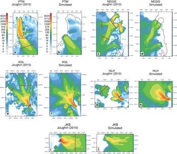
As shown in Section 2.2, the initialization method that we used resulted in modern surface ice velocities, which are broadly in good agreement with Joughin and others (Reference Joughin, Smith, Howat, Scambos and Moon2010). We now analyze the discrepancies in ice velocities between our 20th century simulations and Joughin and others (Reference Joughin, Smith, Howat, Scambos and Moon2010), focusing on the five largest fast-flowing GIS areas: the Petermann glacier (PTM), the NEGIS, the Kangerdlugssuaq glacier (KGL), the Helheim glacier (HLH) and the Jakobshavn glacier (JKB) (Fig. 1d).
The ice stream velocity patterns are generally well captured by GRISLI (Fig. 3). The HLH and KGL glacier regions are the areas where GRISLI shows the best performance (Supplementary Figure S7). GRISLI is able to simulate the multiple-tributary structure of the KGL glacier, which is fed by ice fluxes from three separate valleys that converge in the vicinity of the coast in a single tongue (Figs 3e and f). This good performance results from the spun-up initial topography, which is in very good agreement with Bamber and others (Reference Bamber2013), particularly in these areas (Fig. 1).
(a, c, e, g, i) Observed (Joughin and others, Reference Joughin, Smith, Howat, Scambos and Moon2010) and (b, d, f, h, j) simulated velocities (m a−1) in the five regions studied. In particular (a, b) for the PTM glacier region, (c, d) for the NEGIS region, (e, f) for the KGL glacier region, (g, h) for the HLH glacier region and (i, j) for the JKB glacier region. Note that the grounding lines are drawn for the PTM and NEGIS regions to highlight the location of the floating points. The red lines exhibit the section for the upstream ice flux calculation in each region, likewise the blue lines for the downstream ice flux.

In contrast, compared with Joughin and others (Reference Joughin, Smith, Howat, Scambos and Moon2010), GRISLI underestimates the ice velocities for the JKB glacier (Figs 3i and j), especially downstream where the simulated ice velocities reach ~1.2 km a−1 against ~11 km a−1 in the observations. This discrepancy arises from the horizontal resolution (5 km), which is too coarse to properly capture the narrow valley of the JKB glacier. Aschwanden and others (Reference Aschwanden, Fahnestock and Truffer2016) show that at least a horizontal resolution of 2 km is required to properly capture the JKB glacier valley topography and reproduce its high surface velocities.
Finally, GRISLI is not able to maintain the floating tongue of the PTM glacier and of the NEGIS (Figs 3a–d). There are two reasons for this. Firstly, the floating tongues retreat at the end of the spin-up as a result of the calving criterion, which correspond to a prescribed uniform cutting ice front thickness. GRISLI calculates whether or not the ice fluxes through the grounding line can sustain the floating tongue, if they cannot, or if the front of the floating tongue reaches the cutting thickness value, the front of the floating tongue is calved. Secondly, the inaccuracy in the SMB during the spin-up phase and in the 20th century simulations, stops the floating tongues from growing again (Greve and Herzfeld, Reference Greve and Herzfeld2013). Consequently, GRISLI fails to simulate the velocities and the ice topography in the coastal part of these regions. In contrast, the ice velocities in upstream regions of the PTM glacier and the NEGIS are well simulated by GRISLI (Figs 3a–d, and Supplementary Figure S7).
3.2.2. Projected ice flux evolution up to 2100
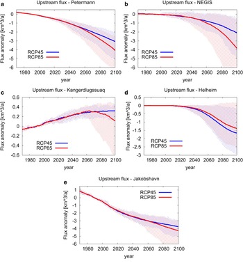
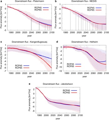
To estimate the future evolution of the ice flux in the five main GIS ice streams, calculations were performed through different vertical sections in each ice stream, one (or two) located upstream (red lines in Fig. 3) and one located downstream near the coasts (blue lines in Fig. 3). For each section, ice fluxes were computed by multiplying the vertical section and the vertically integrated ice velocity perpendicular to the section. In the following analysis, we relate the evolution of the ice fluxes to the variability in ice dynamics and to climate changes, through the equation of continuity  $dH/dt = - \nabla Q + SMB + b_{melt} $ (H = ice thickness; Q = ice fluxes; b melt = basal melting).
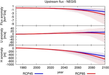
As a result of the simulated negative SMB in the northern half of Greenland during the 21st century, the PTM glacier and the NEGIS ice fluxes decrease upstream (Figs 4a and b), as well as downstream (Figs 5a and b). In fact, the negative SMB causes a retreat of the grounding line of several kilometres inland during the 21st century, which influences the ice flux evolution in these glaciers (Table 3). In the NEGIS region, the ice sheet retreats forever behind the location of the section chosen for the coastal flux calculation by the end of the 21st century (Fig. 5b). Both glaciers exhibit a decreasing trend in ice thickness and ice velocities during the 21st century (Figs 6 and 7). The ice velocity through the upstream section of the NEGIS slightly increases during the 21st century (Fig. 7), due to the ice-sheet retreats (Table 3) and the subsequent steepening of the ice-sheet slopes. This increase in ice velocity, however, is not large enough to counteract the strong reduction in ice thickness resulting from the negative SMB.
Evolution of the fluxes through the upstream sections (red lines in Fig. 3) of the five regions studied: (a) PTM glacier region, (b) NEGIS region, (c) KGL glacier region, (d) HLH glacier region, and (e) JKB glacier region. The values, which are given in  ${\rm km}^{\rm 3} {\kern 1pt} {\rm a}^{ - {\rm 1}} $, cover the period from 1970 to 2100 and are shown as anomalies with respect to the 1980–99 fluxes: ${\rm 7}{\rm. 6}\,{\rm km}^{\rm 3} {\kern 1pt} {\rm a}^{ - {\rm 1}} $ (PTM), ${\rm 15}{\rm. 1}\,{\rm km}^{\rm 3} {\kern 1pt} {\rm a}^{ - {\rm 1}} $ (NEGIS), ${\rm 11}\,{\rm km}^{\rm 3} {\kern 1pt} {\rm a}^{ - {\rm 1}} $ (KGL), ${\rm 10}{\rm. 8}\,{\rm km}^{\rm 3} {\kern 1pt} {\rm a}^{ - {\rm 1}} $ (HLH), ${\rm 20}{\rm. 4}\,{\rm km}^{\rm 3} {\kern 1pt} {\rm a}^{ - {\rm 1}} $ (JKB). The ensemble spreads are shown as dashed areas.

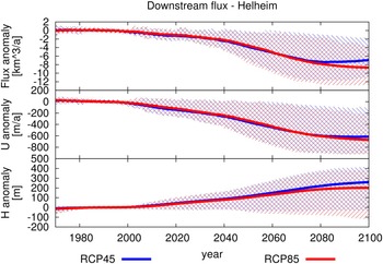
As Figure 4, apart from the fluxes through the downstream sections (blue lines in Fig. 3). The reference 1980–99 ice fluxes are:  ${\rm 4}{\rm. 1}\,{\rm km}^{\rm 3} {\kern 1pt} {\rm a}^{ - {\rm 1}} $ (PTM), ${\rm 3}{\rm. 3}\,{\rm km}^{\rm 3} {\kern 1pt} {\rm a}^{ - {\rm 1}} $ (NEGIS), ${\rm 13}{\rm. 3}\,{\rm km}^{\rm 3} {\kern 1pt} {\rm a}^{ - {\rm 1}} $ (KGL), ${\rm 20}{\rm. 9}\,{\rm km}^{\rm 3} {\kern 1pt} {\rm a}^{ - {\rm 1}} $ (HLH), ${\rm 13}{\rm. 3}\,{\rm km}^{\rm 3} {\kern 1pt} {\rm a}^{ - {\rm 1}} $ (JKB). Note that the black vertical dotted lines in panels (a) and (b) show the years when part of the ice sheet retreats behind the coastal gates.

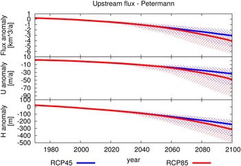
Evolution of ice fluxes ( ${\rm km}^{\rm 3} {\kern 1pt} {\rm a}^{ - {\rm 1}} $), ice velocities (m a−1) and ice thickness (m) in the upstream portion of the PTM glacier. The values cover the period 1970–2100 and are shown as anomalies with respect to the 1980–99 values: ${\rm 7}{\rm. 6}\,{\rm km}^{\rm 3} {\kern 1pt} {\rm a}^{ - {\rm 1}} $ (ice fluxes), 130 m a−1 (ice velocities), and 744 m (ice thickness). The ensemble spreads are shown as dashed areas.

As Figure 6, apart from the upstream portion of the NEGIS. The reference 1980–99 values for the MME are:  ${\rm 7}{\rm. 6}\,{\rm km}^{\rm 3} {\kern 1pt} {\rm a}^{ - {\rm 1}} $ (ice fluxes), 106 m a−1 (ice velocities), and 870 m (ice thickness).

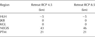
The 21st century grounding line retreat of the GIS (in km) of the front of the five studied ice stream regions

The retreat values correspond to the maximum ice retreat of the ice stream front for each glacier. Note that, given the GRISLI horizontal resolution, a minimum of 5 km retreat or advance is required to be simulated.
Along the eastern coast, the mean simulated SMB remains positive for most of the 21st century, except for the last decades under the RCP 8.5 scenario (Fig. 2). Consequently, both the KGL and the HLH glaciers, which are located in this area, remain stable or advance up to the last decade of the 21st century (Table 3). The KGL glacier exhibits an increase of ~ ${\rm 0}{\rm. 3}\,{\rm km}^{\rm 3} {\kern 1pt} {\rm a}^{ - {\rm 1}} {\rm (\sim\!\! 0}{\rm. 1}\,{\rm km}^{\rm 3} {\kern 1pt} {\rm a}^{ - {\rm 1}} )$ in ice flux along its upstream section during the 21st century under the RCP 4.5 (RCP 8.5) scenario (Fig. 4c). Note that this is the only section of the five fast flowing regions analyzed in our study where simulated ice fluxes increase during the 21st century as a result of an increase in ice velocity (Fig. 8). This acceleration is caused by steepening ice-sheet slopes resulting from positive SMB values and thus increasing ice thickness in the upstream part of this glacier. Conversely, negative SMB and decreasing ice thickness are simulated downstream of the same section (not shown).
As Figure 6, apart from the upstream portion of the KGL glacier. The reference 1980–99 values for the MME are:  ${\rm 5}{\rm. 5}\,{\rm km}^{\rm 3} {\kern 1pt} {\rm a}^{ - {\rm 1}} $ (ice fluxes), 165 m a−1 (ice velocities), and 946 m (ice thickness).

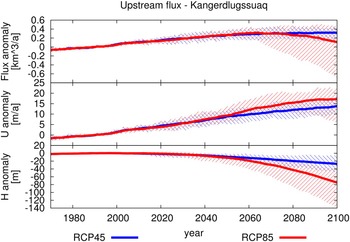
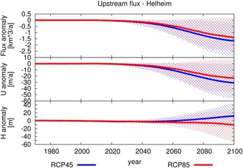
The HLH glacier exhibits a different ice flux evolution compared with the KGL glacier, although both glaciers are located in the same region, and are thus forced by similar climate changes. This different response derives from the differences in the evolution of local SMB, and to the bedrock and fjord geometry (e.g. Joughin and others, Reference Joughin2008b). The upstream section of the HLH glacier is characterized by positive SMB values leading to a small increase in ice elevation (Fig. 9). Therefore, the ice fluxes remain steady through the upstream section (Fig. 4). Due to the buttressing effect created by the bedrock geometry of the fjord (not shown), the amount of ice that reaches the front of the glacier piles up, which increases the ice thickness of the glacier at the front (Fig. 10). This increase in ice thickness at the front, in turn, leads to a reduction in the slope, which results in a reduction in the ice velocities at both upstream and downstream sections during the second half of the 21st century (Figs 9 and 10). This decrease in ice velocities is the main cause for the negative trend in ice fluxes (Figs 4d and 5d). Only in the last decades of the 21st century, is the increase in ice thickness at the downstream section large enough to balance the impact of the decrease in ice velocities, inducing almost steady ice fluxes conditions (Fig. 5d).
As Figure 6, apart from the upstream portion of the HLH glacier. The reference 1980–99 values for the MME are:  ${\rm 10}{\rm. 8}\,{\rm km}^{\rm 3} {\kern 1pt} {\rm a}^{ - {\rm 1}} $ (ice fluxes), 194 m a−1 (ice velocities), and 1408 m (ice thickness).

As Figure 6, apart from the downstream portion of the HLH glacier. The reference 1980–99 values for the MME are:  ${\rm 20}{\rm. 9}\,{\rm km}^{\rm 3} {\kern 1pt} {\rm a}^{ - {\rm 1}} $ (ice fluxes), 1371 m a−1 (ice velocities), and 694 m (ice thickness).

Observations show that the KGL and the HLH glaciers undergo rapid changes in the coastal area due to processes occurring at the calving front (e.g. Joughin and others, Reference Joughin2008b; Nettles and others, Reference Nettles2008; Andresen and others, Reference Andresen2011). Currently, the HLH glacier front is characterized by many calving events (e.g. Joughin and others, Reference Joughin2008b; Nettles and others, Reference Nettles2008), making this glacier one of the most prolific iceberg exporters in Greenland (e.g. Andresen and others, Reference Andresen2011). Furthermore, Andresen and others (Reference Andresen2011) show that the HLH glacier responds to atmosphere-ocean variability on short timescales (3–10 years). In our simulations, small calving events at the front of both glaciers are simulated at a very high frequency (1–2 years) leading to a strong interannual variability in their ice flux evolution at the downstream sections during the 20th and 21st centuries (Figs 5c, d). In fact, GRISLI simulates the fronts of the KGL and the HLH glaciers close to the grounding line, and the absence of a proper description of the grounding line dynamics could explain the high frequency of simulated calving events and the strong instability of these glacier fronts.
Finally, in our simulations, the JKB glacier exhibits a quasi-linear decrease over the 21st century in its upstream region (Fig. 4e), while the coastal section shows a ‘step-like’ evolution (Fig. 5e). In both regions a similar behaviour is simulated under a constant 1980–99 climate (not shown), which indicates that this behaviour is not related to climate changes over the 21st century. Consequently, we relate this behaviour to the horizontal resolution of our grid. In fact, the 5 km horizontal resolution of our simulations inhibits the proper simulation of sub-grid topographic features and, thus, of the JKB glacier dynamics (Fig. 3, and e.g. Aschwanden and others, Reference Aschwanden, Fahnestock and Truffer2016).
To summarize, the ice flux variations during the 21st century are a consequence of SMB changes, which lead to a reduction in ice thickness and the retreat of the GIS in the northern area of Greenland. However, along the eastern coast of Greenland, local topographic features, such as the buttressing resulting from the bedrock geometry in the HLH glacier region, combined with dynamical features, such as the calving events at the front of the HLH and KGL glaciers, determine how the ice flux evolves at the front. Along the western coast, instead, the JKB glacier exhibits changes that reflect the inaccuracy of the coarse 5 km horizontal grid in simulating the geometry of the narrow glacier valley where the JKB glacier lies.
4. DISCUSSION
4.1. Reference climatology
The experiments performed with GRISLI in this work were forced by means of a set of climate forcing from the CMIP5 AOGCM simulations (Taylor and others, Reference Taylor, Stouffer and Meehl2012, and Table 2). The surface air temperature and precipitation used to force our ISM were computed using an anomaly method [Eqn (1)]. The climate simulated by the MAR regional climate model (Fettweis and others, Reference Fettweis2013) is used as a reference for the 20th century. This choice was based on the ability of this model to simulate the Greenland climate compared with observations (e.g. Fettweis and others, Reference Fettweis, Tedesco, van den Broeke and Ettema2011; Franco and others, Reference Franco, Fettweis, Lang and Erpicum2012; Rae and others, Reference Rae2012). However, other climates could be used as reference climatology, such as reanalysis or other regional climate models outputs, for example RACMO (Ettema and others, Reference Ettema2009). For example, when performing the same experiments with ERA Interim global reanalysis as the reference climate, the mean 20th century SMB is ~10 Gt a−1 larger than when using MAR as the reference climate (not shown). This discrepancy is explained by the fact that MAR surface air temperatures are warmer along the GIS margins than in the ERA-Interim (Supplementary Figure S8). The SMB time evolution over the 20th and 21st centuries simulated with the ERA Interim reference climate is similar to that simulated with MAR reference climatology (not shown). In both cases, the MME simulates a reduction of ~7 Gt a−2 (~19 Gt a−2) under the RCP 4.5 (RCP 8.5) scenario. The ice flux evolution up to 2100 in the five main GIS ice streams show similar trends to those using MAR reference climate, although ice fluxes are lower in some of those areas, such as for the HLH glacier, the JKB glacier and the NEGIS. The lower ice fluxes, obtained when using ERA-Interim climate, might result from the low horizontal resolution grid of these climate forcing. In fact, in these main glacier outlets, there is a systematic underestimation of the precipitation compared with MAR (Supplementary Figure S8a). This could be explained by the fact that the lower reanalysis grid resolution does not capture the complex fjord topography of these glaciers. In addition, MAR simulates a warmer climate along Greenland coasts compared with the ERA-Interim (Supplementary Figure S8b and S8c), leading to faster ice velocities and larger ice fluxes in these regions.
4.2. SMB calculation
Our model computes the ablation by a PDD method. Previous studies have shown that the PDD method is more sensitive to temperature variations in warm climates than more physically-based methods, such as the SEBM. For example, van de Wal (Reference van de Wal1996) shows that the sensitivity of a PDD model for a 1°C perturbation in air surface temperature is ~20% higher than the sensitivity of an SEBM. Furthermore, Bougamont and others (Reference Bougamont2007) found that the description of the snow-pack thermo-dynamics has a large impact on the ice-sheet SMB. These discrepancies with the PDD method are mainly due to the fact that the PDD method does not account for albedo changes, and thus does not update surface temperature in relation to the type of glaciated surface (wet snow, dry snow, ice). Therefore, for example, Robinson and others (Reference Robinson, Calov and Ganopolski2010) use the insolation-temperature melt method, based on explicit insolation and albedo changes, which provides more satisfying results of the melt distribution than the basic PDD method. The PDD method also accounts for a fixed and uniform fraction of refreezing of the meltwater, which is the source of the main discrepancy in SMB with the SEBM, together with the lack of radiative feedback, as shown by Bougamont and others (Reference Bougamont2007). However, in Bougamont and others (Reference Bougamont2007), the melting calculation from the PDD and from the SEBM are very similar, and most of the difference comes from the refreezing component.
4.3. Ice-sheet initialization
At the end of our spin-up simulation, our experiments exhibit some biases with respect to observed ice-sheet topography and velocities, especially along the coastal areas, where, for example, the floating tongue of the Petermann glacier and of the NEGIS retreat in our simulations. We attributed these biases to the lack of spatial resolution combined with the effect of the long-term spin-up. To reduce these discrepancies, for example, Edwards and others (Reference Edwards2014) fix the GIS geometry to observed present-day topography (Bamber and others, Reference Bamber2013), then estimate the temperature structure and retrieve the basal drag coefficient from observed ice velocities (Joughin and others, Reference Joughin, Smith, Howat, Scambos and Moon2010) using an iterative inverse method. Finally, Edwards and others (Reference Edwards2014) relax the ice-sheet geometry to the simulated temperature and ice flow fields. Lee and others (Reference Lee, Cornford and Payne2015) show that the use of an inverse method in ice-sheet initialization helps to obtain better model-data agreement. However, in the Edwards and others (Reference Edwards2014) initialization method, the resulting vertical temperature profile and the basal temperature in particular are probably inaccurate since they do not derive from the climate evolution over the last glacial cycle (e.g. Seroussi and others, Reference Seroussi2013). Here, we initialize GRISLI with a free surface simulation forced by an index method in which the ice-sheet basal drag is retrieved using an iterative inverse method (Edwards and others, Reference Edwards2014, and Supplementary Figure S1). This methodology slightly reduces the model-data agreement achievable when using fixed surface and inverse methods together (e.g. Edwards and others, Reference Edwards2014; Lee and others, Reference Lee, Cornford and Payne2015), but it provides a more realistic temperature profile. Consequently, an unique technique to properly initialize ISMs has not yet been found (e.g. Rogozhina and others, Reference Rogozhina, Martinec, Hagedoorn, Thomas and Fleming2011).
The index method also takes into account the impact of a Holocene drift on the ice flux evolution. We evaluate this drift by performing a reference simulation forced by a constant present-day climate (i.e. MAR, 1980–1999, Fettweis and others, Reference Fettweis2013) over the 21st century. The drift amounts to ~36% of the MME ice flux evolution, on average (not shown). For example, this drift drives the ice flux evolution (~80%) in the JKB glacier region (not shown). In contrast, the evolution of ice fluxes in the upstream area of the NEGIS is slightly (~9%) influenced by the spin-up simulation and, consequently, the climatic forcing is the main driver of ice flux evolution in this region (not shown).
4.4. Ocean/ice interactions
In addition to the impact of the spin-up on the outlet of marine glaciers, spatial resolution and various missing processes, such as the treatment of the grounding line dynamics (e.g. Schoof, Reference Schoof2010), hydro-fracturing of the glacier front (e.g. Pollard and others, Reference Pollard, DeConto and Alley2015), or ice/ocean interaction (e.g. Holland and others, Reference Holland, Thomas, Young, Ribergaard and Lyberth2008), limit the ability of our model to simulate the dynamics features of the GIS more accurately. With a 5 km grid, only the largest outlet glaciers are captured properly. As such, in our modelling framework, oceanic warming has only a very limited role for GIS evolution. Note that GRISLI simulates the inland retreat of some of the GIS margins, which also means that probably, in the future, the ocean will not directly impact on the GIS dynamics. However, the complete melting of the Arctic sea ice will lead to regional warming as a result of the subsequent decease in albedo (e.g. Day and others, Reference Day, Bamber and Valdes2013; Fettweis and others, Reference Fettweis2013). Thus, a finer horizontal grid resolution is preferable, as shown by Aschwanden and others (Reference Aschwanden, Fahnestock and Truffer2016) to capture all the topography of the fjords. However, large uncertainties in ocean-induced basal melting parametrizations due to the lack of marine observations from the fjords, and in the buttressing process limit the modelling impact of the use of finer horizontal grid resolutions. In addition, the simulation of a climate forcing at a comparable resolution with that of the ISM used is necessary to properly reproduce the dynamics of the fjord glaciers.
4.5. GRISLI basal drag
Our simulations were developed by assuming a constant basal drag over the 20th and 21st centuries. This assumption derives from the lack of any meltwater infiltration scheme in GRISLI that is able to redirect surface meltwater from the surface to the ice-sheet base, where it could increase the basal lubrication and thus modify ice-sheet velocities (e.g. Zwally and others, Reference Zwally2002). Fürst and others (Reference Fürst, Goelzer and Huybrechts2015) show that the effect of enhanced basal lubrication on the ice volume evolution is negligible on centennial timescales. However, infiltration models have been developed and applied at the regional scale (e.g. Clason and others, Reference Clason, Mair, Burgess and Nienow2012; Banwell and others, Reference Banwell, Willis and Arnold2013; Clason and others, Reference Clason2015), and their implementation in the ISMs could be of interest for future work.
4.6. Hybrid model limitations
GRISLI is a hybrid model (e.g. Kirchner and others, Reference Kirchner, Hutter, Jakobsson and Gyllencreutz2011), and is based on SIA and SSA, which restrict its ability to resolve the dynamics in complex topography areas, such as the fjords located along the coasts of the GIS, which are also poorly resolved with a 5 km resolution grid. Higher-order or full-Stokes ISMs could overcome some of these limitations. However, higher-order or full-Stokes models cannot be run in the long-term, for example for paleoclimate spin-up simulations (Gillet-Chaulet and others, Reference Gillet-Chaulet2012; Seddik and others, Reference Seddik, Greve, Zwinger, Gillet-Chaulet and Gagliardini2012) due to their high demand on computational resources.
Despite various dynamical limitations, a hybrid ISM can be run over multiple timescales under a large variety of climate forcing and physical parametrizations, thus enabling the sources of uncertainty to be evaluated. In addition, SIA/SSA ISMs satisfactorily simulate present-day and future GIS conditions compared with more complex ISMs (e.g. Edwards and others, Reference Edwards2014). For example, in the case of the main drainage areas, such as the NEGIS, SIA, hybrids, higher-order and full-Stokes all fail to accurately reproduce the observations (e.g. Goelzer and others, Reference Goelzer2013; Greve and Herzfeld, Reference Greve and Herzfeld2013).
Finally, future ISM development, especially for fast flowing areas, should include upgraded model physics, increased resolution, and better floating outlet glacier termination representation.
5. CONCLUSION
In the present study, we analyzed the evolution of the ice fluxes of five ice streams and outlet glaciers. The evolution of the ice dynamics was computed using a hybrid ISM, i.e. GRISLI, which simulates a 20th century SMB amplitude and distribution, as well as ice velocity patterns in good agreement with observations and the literature.
In agreement with previous works (e.g. Yan and others, Reference Yan, Wang, Johannessen and Zhang2014; Fürst and others, Reference Fürst, Goelzer and Huybrechts2015), GRISLI simulates a mean present-day SMB of ~212 Gt a−1 (170–469 Gt a−1, literature range), and a mean cumulative decrease of ~10 cm SLE (~20 cm SLE) by 2100 under the RCP 4.5 (RCP 8.5) scenario. However, GRISLI overestimates ablation due to the sensitivity of the PDD method to warm climate conditions.
In general, our results confirm that the SMB evolution is the main driver of the evolution of the GIS over the 21st century. Nevertheless, local scale dynamical features have a significant influence on the interannual variability and on the local ice flux evolution.
Along the eastern coast, the simulated ice flux trends are mostly dominated by climate change up to 2100. However, the calving events and oscillations in the sliding velocities lead to a strong interannual variability of Kangerdlugssuaq and Helheim glacier outlets. Along the western coast, the simulated ice flux evolution in the Jakobshavn glacier region reflects the inaccuracy of the coarse 5 km horizontal grid in simulating the geometry of the narrow glacier valley where the Jakobshavn glacier lies, and, thus, its dynamics.
In the northern area, the GIS is characterized by negative SMB values, which lead to a retreat of the ice sheet in these regions by the end of the 21st century, as shown by the decrease in the ice flux evolution simulated in the Petermann glacier and NEGIS regions.
Finally, in our simulations, the changes in the GIS topography, such as the ice margin retreat and changes in the ice-sheet slopes, triggered by climate changes during the 21st century, exhibit a significant impact on the future GIS evolution, especially in the fast flowing areas.
AUTHOR CONTRIBUTION
Daniele Peano designed and performed the experiments, analyzed the outputs and wrote the manuscript; Florence Colleoni discussed the design of the experiments, discussed the results and participated in the writing; Aurélien Quiquet discussed the design of the experiments, discussed the results and participated in the writing; Simona Masina discussed the results and participated in the writing.
SUPPLEMENTARY MATERIAL
The supplementary material for this article can be found at https://doi.org/10.1017/jog.2017.12
ACKNOWLEDGEMENTS
We thank Catherine Ritz, who provided the GRISLI ice-sheet model code. We also thank Xavier Fettweis who shared the MAR outputs with us, and Nina Kirchner who helped in developing the initialization simulations and whose comments improved the manuscript. We thank the two anonymous reviewers whose comments also improved the manuscript. We acknowledge the CMCC foundation for providing the supercomputer on which the simulations were performed.


 Open access