


1. Introduction
Economists have increasingly resorted to social norms – shared understandings of actions that are appropriate or inappropriate in a given context – to explain a wide range of behaviors and outcomes, including prosociality (Kimbrough & Vostroknutov, Reference Kimbrough and Vostroknutov2016), honesty (Aycinena et al., Reference Aycinena, Rentschler, Beranek and Schulz2022), discrimination (Barr et al., Reference Barr, Lane and Nosenzo2018), law obedience (Lane et al., Reference Lane, Nosenzo and Sonderegger2023), and gendered outcomes in labor markets (Bursztyn et al., Reference Bursztyn, González and Yanagizawa-Drott2020). In recent years, scholars have introduced and refined a number of experimental techniques to measure social norms (e.g., Bicchieri & Xiao, Reference Bicchieri and Xiao2009; Krupka & Weber, Reference Krupka and Weber2013; Dimant, Reference Dimant2023; Aycinena et al., Reference Aycinena, Bogliacino and Kimbrough2024a; Panizza et al., Reference Panizza, Dimant, Kimbrough and Vostroknutov2024, see Görges & Nosenzo, Reference Görges and Nosenzo2020 for a review). With 1,343 Google Scholar citations at the time of writing and a placement in the top 1‰ of research papers by number of citations in the RePEc/IDEAS database, the method introduced by Krupka and Weber Reference Krupka and Weber(2013) is arguably the most popular in current economics research.
In the Krupka-Weber (KW) method, experimental subjects are given a description of a situation in which behavior takes place. Subjects then rate the social appropriateness of the behavior in the situation, based on what they perceive to be the most common rating provided by other participants completing the same task. Subjects obtain a monetary reward if they succeed in rating the behavior in the same way as most other participants. In this paper, we provide a comprehensive evaluation of the role of monetary incentives in the KW method across three studies involving 5,114 participants.
Studying the effect of incentives in the KW task is particularly interesting because monetary incentives can influence responses in a number of different ways – some of which are desirable, while others may be undesirable. A first-order desirable effect may be that, when participants obtain a monetary reward based on their responses in the task, the quality of responses increases. This could be the result of a number of factors, ranging from increased time and attention devoted to the task, to a better understanding of the task itself. Incentives may specifically improve understanding by making it salient to participants that their goal in the task is not to provide their own personal assessment of the appropriateness of behavior, but instead to match the responses of others, thereby revealing their perception of the social norm (on this point see Krupka & Weber, Reference Krupka and Weber2013, pp. 498–501).
However, the use of incentives in the KW task has also been criticized on the basis that, while incentives encourage participants to tacitly coordinate responses with others, there is no guarantee that participants will use their perception of the social norm to do so. In principle, participants could use any focal point present in the decision task to coordinate, even if it is not related to the social norm. Thus, the use of monetary incentives may inadvertently provide subjects a reason to not reveal the perceived social norm, if another, more salient coordination point is available in the elicitation task.Footnote 1 The influence of such a “focal point distortion” has been assessed recently by Fallucchi and Nosenzo Reference Fallucchi and Nosenzo(2022) and Aycinena et al. (Reference Aycinena, Bogliacino and Kimbrough2024c), who find little evidence for it. In this paper, we provide a new test of this potential distortion, comparing its severity in the presence and absence of monetary incentives for coordination.
A further concern is that monetary incentives may shift the balance between the motivational goals and values that individuals take into account when forming their opinions and decisions.Footnote 2 Kasser Reference Kasser(2016) reviews experimental research showing that activation of financial goals promotes materialistic attitudes and behavior. Mere reminders of, or exposure to, money have been found to promote materialism, although some of these results have not been replicated (e.g.,Caruso et al., Reference Caruso, Vohs, Baxter and Waytz2013; Rohrer et al., Reference Rohrer, Pashler and Harris2015). A possible conjecture is that incentives may introduce a “materialistic bias” in the norms elicited with the KW task, increasing the reported acceptability of materialistic profit-seeking behaviors.
In Study 1 ( $\mathrm{N} = 1,105$), we analyze the effect of monetary incentives on response quality, focal point distortion and materialistic bias. We use a vignette experiment where subjects read descriptions of behavior in fictitious decision situations and rate its appropriateness. Subjects are instructed to rate behavior according to their perception of the most common appropriateness rating given by other participants in the experiment. In one treatment, subjects are paid if they successfully match the most common rating, while in another treatment they receive no monetary reward for matching. Our results show no evidence of focal point distortion or materialistic bias in the KW task in the presence of monetary incentives. Moreover, while response quality (as measured by time spent on the task, attention to task details, and correct understanding of the task) is slightly higher in the condition with incentives, we find no statistically significant differences in any of these outcomes between incentivized and unincentivized conditions.
In two subsequent studies, we explore additional sources of bias that researchers often worry about in opinion tasks, and gauge their prevalence in the KW task. The first bias, which we refer to as “moral hypocrisy”, is the concern that participants may report their perception of the social norm in a way that self-servingly rationalizes behavior or outcomes that are materially advantageous to oneself. This tendency has been reported in related choice and opinion tasks where individuals redistributed money between themselves and others, and/or expressed judgments about the fairness of different distributions of outcomes (e.g., Konow, Reference Konow2000, Reference Konow2005; Dana et al., Reference Dana, Lowenstein, Weber, Cremer and Tenbrunsel2011). For example, in a classic study described in Dana et al. Reference Dana, Lowenstein, Weber, Cremer and Tenbrunsel(2011), subjects chose how to split a reward between themselves and another participant as compensation for work in a task. Across conditions, the experiment varied whether the subject or the other participant was more deserving of the reward and found that subjects’ choices appeared to reflect fairness principles chosen selectively to best suit their material interest. Similarly, Rustichini and Villeval (Reference Rustichini and Villeval2014) found that subjects distorted their (unincentivized) fairness views about behavior in Dictator, Ultimatum, and Trust games, aligning them with the actions they themselves had previously taken in these games.
Building on these literatures, in Study 2 ( $\mathrm{N} = 2,512$) we report an experiment where subjects were asked to evaluate the social appropriateness of a relative-performance pay criterion for a real-effort task they had previously taken part in. We randomly assigned subjects to treatments in which the pay criterion was either materially advantageous or disadvantageous to them. In one version of the experiment, we did not incentivize subjects’ social appropriateness ratings. In another version, we used the standard KW incentives (subjects are paid if they successfully match the most common rating among other respondents). In the unincentivized condition, we find a significant gap in social appropriateness ratings between subjects who would be advantaged by the pay criterion and those who would be penalized by it. The gap closes completely when we use the incentivized KW task.
Finally, we explore the possibility that norm elicitations may be vulnerable to “interviewer bias”. In the context of norm elicitation tasks, a concrete concern is that in settings where respondents perceive a conflict between the social norm within their reference group and the social norm they believe is upheld by the interviewer, they may align their evaluations with the interviewer’s perceived norm rather than accurately reflecting their group’s actual norm (Görges & Nosenzo, Reference Görges and Nosenzo2020; Aycinena et al., Reference Aycinena, Bogliacino and Kimbrough2024b).
In the experiment reported in Study 3 ( $\mathrm{N} = 1,497$), we focus on the potential bias that may arise from the observable sex of the interviewer. Specifically, we randomly allocate subjects to treatments where, at the outset of the task, they are introduced to either a male or a female researcher. We then ask subjects to rate the social appropriateness of behavior in vignettes where – based on the results of a manipulation check – men and women are perceived to hold different normative views. We do not incentivize subjects’ responses. We find no evidence of interviewer bias in social appropriateness ratings.
The results of our three studies complement the existing evidence on the effects of incentives in norm elicitation tasks. We are aware of four previous papers. Veselý Reference Veselý(2015) compares incentivized and unincentivized measurements of norms in the Ultimatum game using the KW method with a sample of 270 university students. He reports no differences in ratings of appropriateness across incentivized and unincentivized conditions. Groenendyk et al. Reference Groenendyk, Kimbrough and Pickup(2023) use the Krupka–Weber technique to compare perceived norms about policy positions among self-identified liberals and conservatives in the U.S. in a sample recruited via YouGov. The experiment includes both incentivized (467 subjects) and unincentivized (494 subjects) norm elicitations. They report only limited evidence of a reduction in response noise under incentivization. König-Kersting Reference König-Kersting(2024) compares ratings of appropriateness in the Dictator game elicited across different versions of the KW task, including versions with and without monetary incentives. In a sample of 1,228 Amazon Mechanical Turk participants allocated across 12 treatments, he finds no differences in ratings between incentivized and unincentivized conditions. Finally, Huffman et al. Reference Huffman, Kohno, Madies, Vogrinec, Wang and Yagnaraman2024 compare appropriateness ratings in Give and Take versions of the Dictator game elicited using different norm-elicitation techniques (e.g., Bicchieri & Xiao, Reference Bicchieri and Xiao2009; Krupka & Weber, Reference Krupka and Weber2013), using a sample of 751 Prolific participants randomized across 10 conditions. They include versions of these techniques with monetary incentives to match others’ ratings and versions without incentives, and find no differences across conditions.
Our paper complements and extends these studies in several key ways. First and foremost, we articulate several distinct channels through which incentives may affect responses in the KW task, ranging from effects on response quality to several biases that have been discussed in relation to norm-elicitation and opinion tasks. Our three studies were specifically designed to stress-test these different potential effects of incentives, thus providing the most comprehensive evidence to date on the role of incentives in KW norm-elicitation tasks. Second, our studies elicit social norms in a wider range of situations than the simple distributional games studied in most previous papers. Finally, we utilize substantially larger sample sizes than most previous studies. Only Groenendyk et al. Reference Groenendyk, Kimbrough and Pickup(2023) ran experiments with a sample size comparable to ours, whereas the samples used by Veselý Reference Veselý(2015), König-Kersting Reference König-Kersting(2024), and Huffman et al. Reference Huffman, Kohno, Madies, Vogrinec, Wang and Yagnaraman2024 are considerably smaller (around one-quarter the size of ours). Our tests are based on a median sample size of nearly 500 subjects per condition, which allows us to rule out effects of reasonably small magnitude and reduces the risk of false positives.
While previous studies had found neutral effects of incentives in norm elicitation tasks, our paper paints a more nuanced picture – showing that it is important to consider the potential mechanisms at play in social norm elicitation tasks in order to evaluate how incentives influence the elicitation of norms. In line with the neutrality results of previous papers, we find that incentives do not affect responses in the direction of norm-unrelated focal points or materialistic values, and that they only yield modest gains in terms of response quality. However, incentives do seem to play a role in correcting response biases that may occur in norm-elicitation tasks. These biases may not always be present in the absence of incentives (as our data from Study 3 reveal), but when they are present, incentives appear to mitigate (and, in the case of Study 2, completely eliminate) these distortions, providing a more accurate elicitation of underlying social norms.
2. Study 1: response quality, focal point distortion and materialistic bias
The main focus of the study is to test whether incentives affect response quality, focal point distortion and materialistic bias. We pre-registered the experiment on OSF (also reproduced in Appendix A), and all hypotheses, exclusion criteria, and analyses reported below follow the pre-registration, unless explicitly stated otherwise. The experiment was programmed using the software SurveyXact and was conducted online in December 2024 using participants recruited from Prolific UK (none of the participants took part in any of our other studies).
2.1. Design
The study began with a screen giving participants general information about the nature of the study (purpose, data confidentiality, funding, etc.) and asking for their consent to take part in it. Subjects then read the experiment instructions (reproduced in Appendix B). They learned that the study consisted of three vignettes describing situations in which a person takes an action. Their task was to rate the social appropriateness of the behavior described in each of the three vignettes. We defined social appropriateness as “behavior that [they thought] most other Prolific participants from the UK would agree is the right thing to do”.
The second screen of the instructions contained our treatment manipulation. Subjects were randomly assigned to either the NoIncentive or the Incentive treatment. All subjects were told that we would recruit other participants to take part in the same experiment, and that their task was to rate the appropriateness of behavior in each vignette to match the most common rating given by these other participants.
Subjects in the Incentive condition were further told that they could earn a bonus of 1 GBP for each vignette where their appropriateness rating matched the most common rating by other participants (standard KW incentive scheme). Thus, subjects in the Incentive treatment could earn up to 3 GBP in the experiment, which is a very high incentive in our setting (average task duration was approximately 5 minutes, which implies a corresponding hourly wage of 36 GBP).Footnote 3 The additional information slightly increased the length of the text shown on the screen. Importantly, this was the first time that subjects learned they could earn a bonus in the experiment. The recruitment letter did not mention any bonus, but only a guaranteed participation fee of 0.60 GBP. This was done in order to keep the recruitment procedures constant across treatments, thus avoiding potential selection into treatment.
Before proceeding to the vignettes, subjects were given an opportunity to re-read the instructions and then asked a control question about the task. The control question read: “Which of the following four statements about the task is true?”, and subjects answered choosing one of the following options:
(a) “My task is to rate the appropriateness of behavior according to my own personal opinion of what is the right thing to do”.
(b) “My task is to rate the appropriateness of behavior to match the most common appropriateness rating given by other UK Prolific participants”.
(c) “My task is to rate the appropriateness of behavior according to what is legal or illegal in the UK”.
(d) “My task is to rate the appropriateness of behavior according to how common the behavior is in the UK”.
The correct answer was (b) in both treatments. Subjects had only one attempt at answering the question. Regardless of how they answered, the subsequent screen reminded all subjects about the correct answer before proceeding further with the experiment.
Subjects then read the three vignettes, each appearing on a separate screen. The first vignette (“Beggar vignette”) described a doctor ignoring a beggar who had approached him to ask for money. The second vignette (“Drug Price vignette”) described a pharmaceutical company raising the price of a drug in response to an exogenous shift in demand triggered by the drug being found effective for a new condition. The third vignette (“Wallet vignette”) described a student picking up a lost wallet in a coffee shop and walking out with it. The three vignettes were shown to participants in the same order as discussed above.Footnote 4 In each screen, subjects were also reminded of the meaning of the term “social appropriateness”. Subjects in the Incentive treatment were further reminded of the possibility of earning 1 GBP for matching the most common rating by other participants in the vignette.
Responses were collected on a four-point scale from “Very socially appropriate” to “Very socially inappropriate”. In the first two vignettes, the scale was ordered top-to-bottom from “Very socially appropriate” to “Very socially inappropriate”. In the third vignette, unannounced to the subjects, the scale appeared in reversed order (from “Very socially inappropriate” to “Very socially appropriate”).
After the third vignette, subjects were asked a “surprise” recall question about a specific detail in that vignette and were promised an extra monetary incentives of 0.50 GBP if they responded correctly within 20 seconds.Footnote 5 The question read: “In the situation you just read, what time was displayed on the clock in the coffee shop?”, and subjects answered choosing between (a) “Just before noon”, (b) “Noon”, (c) “Just past noon”, or (d) “The situation did not mention a clock”. The correct answer was (c).
The experiment concluded with the collection of basic socio-demographic information (gender, age, education, income, family composition, employment status, country of birth).
2.2. Hypotheses and outcome variables
Our hypotheses concern the effects of monetary incentives on responses quality, focal point distortion, and materialistic bias. Specifically, we have the following directional hypotheses:
H1: Response quality is higher in the Incentive than NoIncentive treatment;
H2: Focal point distortion is larger in the Incentive than NoIncentive treatment;
H3: Materialistic bias is larger in the Incentive than NoIncentive treatment.
Our outcome variables are as follows. For H1, we have four different outcomes, capturing different aspects of the quality of responses. First, we consider task duration, measured as the time subjects spent between the first and the last page of the study. We hypothesized that subjects in the Incentive treatment would spend longer time in the experiment compared to the NoIncentive treatment.Footnote 6
Second, we focus on understanding of the KW task. We do so by computing the fraction of subjects who answered correctly the control question described above. We hypothesized that the proportion of correct answers would be higher in the Incentive than NoIncentive treatment.
Third, we have two measures of task attention. First, we consider the fraction of subjects who answer correctly the surprise recall question about the Wallet vignette. We hypothesized that the proportion of correct answers would be higher in the Incentive than NoIncentive treatment. Second, we consider the distribution of ratings in the Wallet vignette. Recall that in this vignette, unbeknownst to subjects, we reversed the order of the response scale. This should not affect the response behavior of subjects who are attentive to the task, but may however reverse the responses of inattentive subjects.Footnote 7 We hypothesized that the fraction of inattentive subjects would be lower in the Incentive than NoIncentive treatment, which can be detected as a difference between treatments in the distribution of ratings in this vignette.
For H2, our outcome variable is the distribution of ratings in the Beggar vignette. We introduced a focal coordination point in the text of the vignette by explicitly mentioning that the vignette protagonist had read an article suggesting that “... it is considered very socially appropriate to ignore beggars who ask for money on the street”. The use of a sentence explicitly mentioning an appropriateness level in the text of the vignette may serve as a cue for subjects to coordinate their ratings with others when answering the question: “How socially appropriate do you think most people would find the doctor’s decision to ignore the beggar?”.Footnote 8 We hypothesized that a larger fraction of subjects may use this cue in the Incentive than NoIncentive treatment (focal point distortion), resulting in a positive shift in the distribution of ratings (i.e., towards higher appropriateness) in the Incentive treatment.
For H3, our outcome variable is the distribution of ratings in the Drug Price vignette. The vignette describes profit-maximizing behavior by a pharmaceutical firm that raises the price of a drug following an exogenous increase in demand. Our conjecture was that, if the presence of monetary incentives in the KW task strengthens the focus on materialistic profit-seeking goals, then subjects may view the firm’s profit-maximizing response as more appropriate in the Incentive than NoIncentive treatment – a pattern we refer to as materialistic bias.Footnote 9 This bias may manifest as a positive shift in the distribution of ratings (i.e., towards higher appropriateness) in the Incentive treatment.
2.3. Implementation
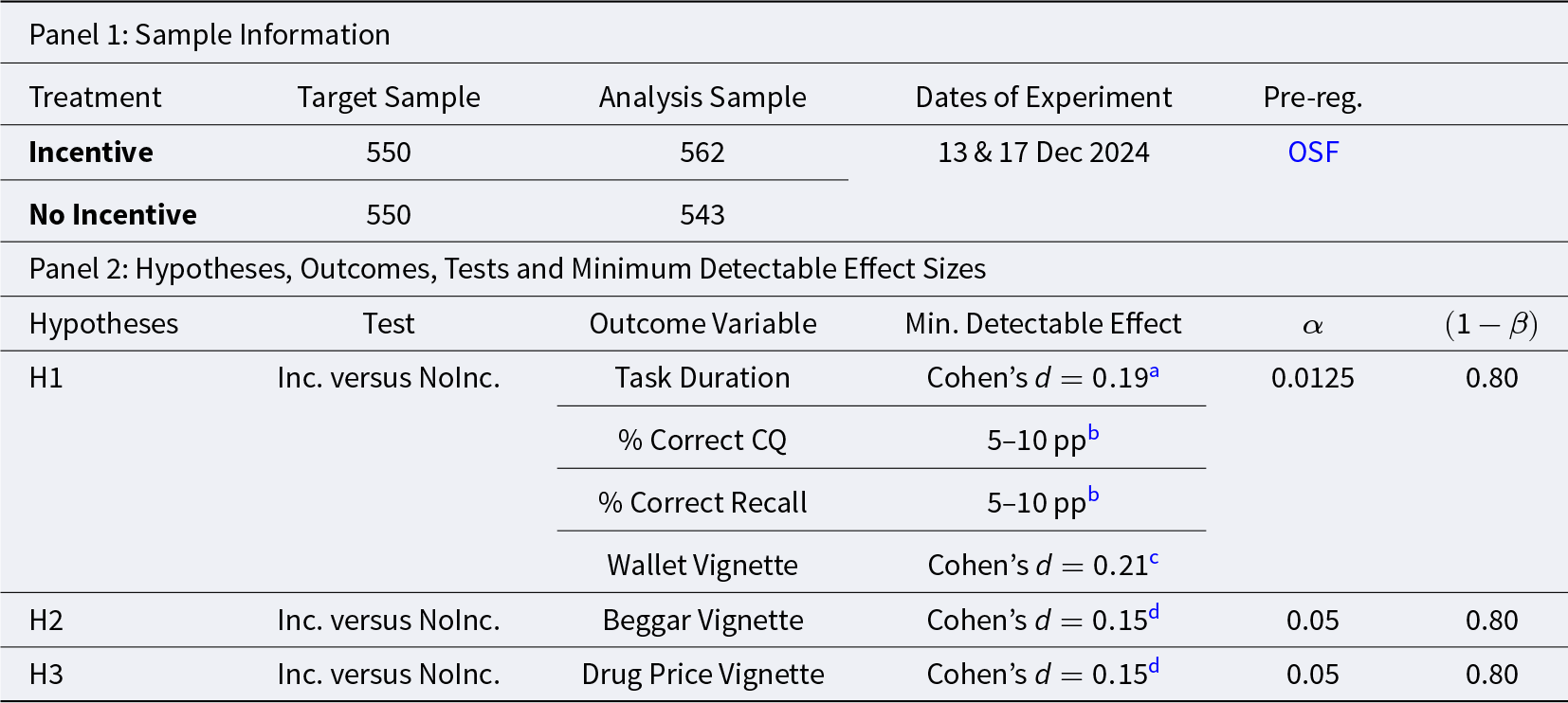
We collected a total of 1,270 observations from 1,199 participants recruited from Prolific UK. After excluding participants who started the experiment more than once and those who did not complete it, we retain 1,105 participants as the sample for analysis.Footnote 10 Of these, 543 were randomly assigned to the NoIncentive treatment and 562 to the Incentive treatment. Table 1 presents the minimum detectable effect sizes and associated power of each of our tests.
Study 1 – sample size and power
Notes: Cohen’s  $d$ refers to the absolute magnitude of the standardized mean difference; that is,
  $|d|$ values are reported without regard to direction.
a Based on one-sided t-test of differences in seconds taken to complete the experiment;
b Based on one-sided test of differences in proportions;
c Based on two-sided rank-sum test of differences in appropriateness ratings;
d Based on one-sided rank-sum test of differences in appropriateness ratings.  $\alpha$ indicates the significance level used in the tests;
  $(1-\beta)$ indicates the statistical power. The minimum detectable effect sizes for H1 have been computed conservatively, by committing to a significance level of
  $\alpha = 0.0125$ in each test to account for the use of four different outcome variables (Multiple Hypothesis Testing correction). The minimum detectable effect sizes are computed for a target sample size of 550 subjects per treatment, as per our pre-registration.
2.4. Results
2.4.1. H1: response quality
Figure 1 summarizes the four outcome variables measuring response quality in the Incentive and NoIncentive treatments. Starting with task duration (top-left panel), in line with our hypothesis, we observe an increase in the number of seconds spent in the experiment in the Incentive treatment (avg. 320, s.d. 203) compared to NoIncentive (avg. 305, s.d. 236). The effect is however small, corresponding to a Cohen’s d of 0.068 (95% confidence interval between −0.050 and 0.186). Based on a one-sided t-test we cannot reject the null hypothesis of no difference in time spent in the task between treatments ( $\mathrm{t} = 1.137$; one-tailed p-value
  $ = 0.128$; adjusted for MHT using the Benjamini–Hochberg False Discovery Rate method: 0.128).
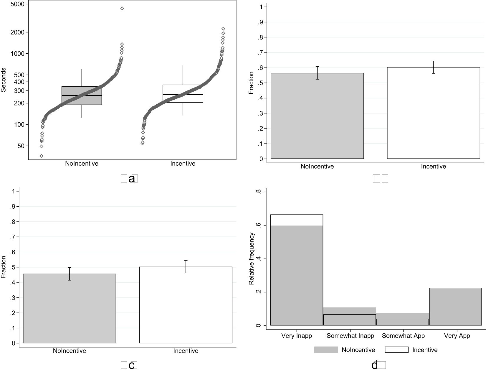
Response quality (a) task duration (b) % correct control question (c) % correct recall (d) appropriateness ratings wallet vignette

The top-right panel shows the percentage of subjects who answered correctly the control question about the nature of the KW task. In the NoIncentive treatment, 57% of subjects selected the correct answer compared to 60% in the Incentive treatment. The increase in proportion of correct answers is in line with our hypothesis, but the effect is small and we cannot reject the null of no difference between treatments using a test of proportions ( $\mathrm{z} = 1.276$; one-tailed p-value
 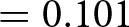 $ = 0.101$; adjusted for MHT: 0.128).
The bottom-left panel shows the percentage of subjects who answered correctly the surprise recall question about the Wallet vignette. In the NoIncentive treatment, 46% of subjects selected the correct answer, compared to 50% in the Incentive treatment. This increase is again in line with our hypothesis, but the effect is small and we cannot reject the null of no differences between treatments using a test of proportions (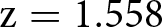 $\mathrm{z} = 1.558$; one-tailed p-value
 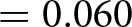 $ = 0.060$; adjusted for MHT: 0.128).
Finally, the bottom-right panel shows the distribution of ratings in the two treatments for the Wallet vignette, where the response scale order was reversed. Following convention in the social norms literature, we assign evenly-spaced values of +1 to the rating “Very socially appropriate”, +0.33 to “Somewhat socially appropriate”,  $-$0.33 to “Somewhat socially inappropriate”, and
  $-$1 to “Very socially inappropriate”. The two distributions are very similar. The corresponding Cohen’s d is
  $-$0.069 (95% confidence interval between −0.187 and 0.049). We cannot reject the null hypothesis that the two distributions are the same using a rank-sum test (
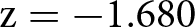 $\mathrm{z} = -1.680$; two-tailed p-value
 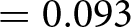 $ = 0.093$; adjusted for MHT: 0.128).
2.4.2. H2 & H3: focal point distortion and materialistic bias
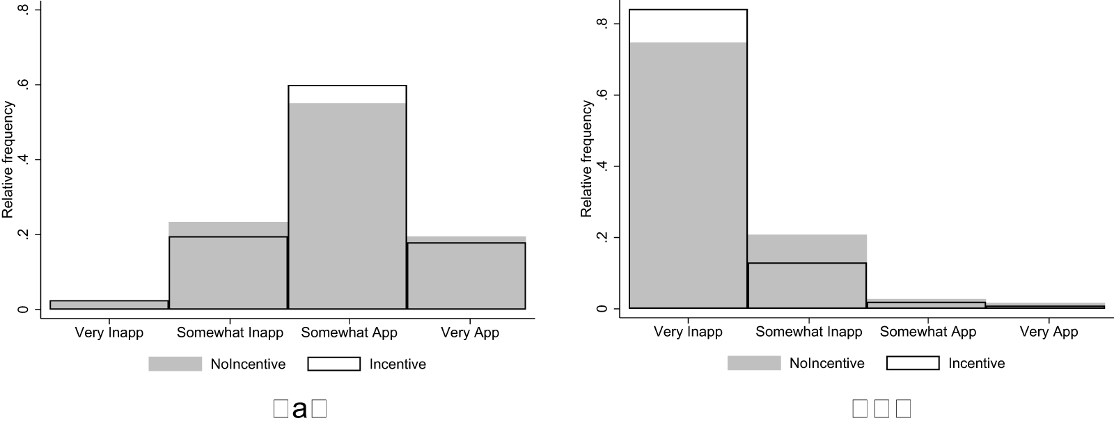
Figure 2 shows the distribution of ratings across the two treatments in the Beggar and Drug Price vignettes, which we use to test hypotheses H2 and H3. Starting with H2, we hypothesized that a focal point distortion would result in a positive shift (towards higher appropriateness) in the distribution of ratings of the Beggar vignette in the Incentive treatment compared to NoIncentive. We observe a small positive shift, with average appropriateness increasing from 0.279 (s.d. 0.472) in the NoIncentive treatment to 0.288 (s.d. 0.457) in the Incentive treatment. This corresponds to a Cohen’s d of 0.019 (95% confidence interval between -0.099 and 0.136). We cannot reject the null hypothesis that the two distribution are the same using a rank-sum test (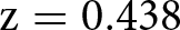 $\mathrm{z} = 0.438$; one-tailed p-value
 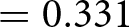 $ = 0.331$).
Distribution of Ratings in the Beggar (a) and Drug Price (b) Vignettes

For H3, we hypothesized that a materialistic bias would produce a positive shift in the distribution of ratings of the Drug Price vignette in the Incentive treatment compared to NoIncentive. We actually observe a shift in the opposite direction, with average appropriateness decreasing from −0.791 (s.d. 0.406) in the NoIncentive treatment to −0.869 (s.d. 0.334) in the Incentive treatment. This corresponds to a Cohen’s d of −0.211 (95% confidence interval between −0.329 and −0.093), but the effect goes in the opposite direction of our hypothesis. Therefore, we cannot reject the null hypothesis that the two distributions are the same using a one-sided rank-sum test ( $\mathrm{z} = -3.849$; one-tailed p-value
  $ = 0.999$).
All results are robust to additional regression analysis including socio-demographic controls (see Appendix E for details). Overall, we fail to detect significant effects of incentives in the KW task across all our outcome variables, finding support for none of our hypotheses.
3. Study 2: moral hypocrisy
The main focus of Study 2 is to test for the influence of moral hypocrisy in social norm elicitation tasks. We pre-registered the experiment on OSF (reproduced in Appendix F) and all hypotheses, exclusion criteria and analyses reported below follow the pre-registration unless explicitly noted otherwise. The experiments were programmed using the software SurveyXact and conducted online between December 2024 and January 2025 using participants recruited from Prolific UK (none of the participants took part in any of our other studies).
3.1. Design
Subjects were recruited to take part in a transcription task for a guaranteed participation fee of 0.65 GBP plus a potential additional monetary bonus of 0.50 GBP. After providing informed consent for the study, subjects read the task instructions (reproduced in Appendix G). Participants learned that in the task they would transcribe 10 alphanumeric strings. They also learned that their performance in the task would be compared to that of another participant who had completed the same task (these were actual subjects recruited in a pilot to perform the same transcription task as in the main study). They were told that the monetary bonus of 0.50 GBP would be awarded to either them or the other participant, with further details provided at the end of the task.
At the end of the task, participants saw a comparison of their performance in the transcription task relative to the other participant. Each subject who had correctly transcribed between 1 and 9 strings was randomly assigned to see either a favorable performance comparison (indicating they had transcribed more strings correctly than the other participant) or an unfavorable performance comparison (indicating they had transcribed fewer strings correctly than the other participant). This information was truthful since participants were selectively matched with previous participants who had performed worse or better than the subject in the same transcription task.Footnote 11 We call the former treatment BETTER and the latter WORSE.
Subjects were then asked to consider the possibility that we would award the 0.50 GBP transcription task bonus to them or the other participant based on their relative performances in the task. Subjects were asked to rate the social appropriateness of this potential performance-based criterion to award the bonus.Footnote 12
Before rating the criterion, subjects read instructions explaining the norm-elicitation task (this was the standard KW task, asking subjects to match the most common social appropriateness rating among other respondents), and answered a control question about it.Footnote 13 In one version of the experiment (Incentive condition) subjects were paid an additional bonus of 1 GBP for matching the modal rating, while in the other version they were not (NoIncentive condition).Footnote 14 Responses were collected on a four-point scale from “Very socially appropriate” to “Very socially inappropriate”.
After rating the criterion, subjects were informed that we had ultimately decided not to use the performance-based criterion for the transcription task. Instead, they were told that they would receive the £ $0.50$ bonus regardless. The experiment concluded with a set of questions eliciting the same socio-demographic information as in Study 1.
3.2. Hypotheses and outcome variables
We hypothesized that subjects who were shown an unfavorable performance comparison (WORSE treatment) would be more likely to self-servingly report a norm against relative performance-based pay compared to subjects in the BETTER treatment.Footnote 15
We test this directional hypothesis by comparing social appropriateness ratings of the relative performance-based pay criterion between the WORSE and BETTER treatments. We test this separately in the NoIncentive and Incentive versions of the norm elicitation task. We also test for differences in moral hypocrisy bias between the NoIncentive and Incentive conditions, by conducting a diff-in-diff analysis.
3.3. Implementation
The study was run across three data collection waves on Prolific UK. Table 2 provides details about sample sizes and power of the analyses for each data collection wave.
Study 2 – Sample Size and Power
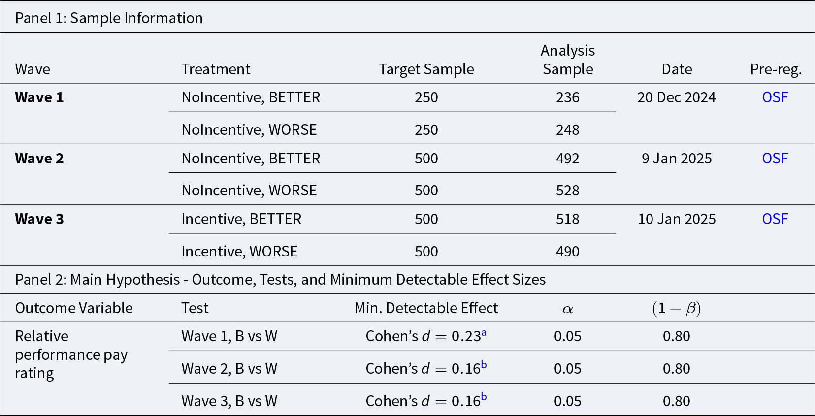
Notes: Cohen’s  $d$ refers to the absolute magnitude of the standardized mean difference; that is,
  $|d|$ values are reported without regard to direction.
a Based on one-sided rank-sum test of differences in appropriateness ratings with the target sample size of 250 subjects per treatment.
b Based on one-sided rank-sum test of differences in appropriateness ratings with the target sample size of 500 subjects per treatment.  $\alpha$ indicates the significance level used in the tests;
  $(1-\beta)$ indicates the statistical power.
In Wave 1 we collected 516 observations in the NoIncentive condition, of which 484 were unique and complete and were retained for analysis. This sample size reflects a partial data collection that was halted after an interim analysis – pre-registered as part of a sequential sampling strategy – showed the effect size was too small to conduct the planned analysis with adequate statistical power, and thus did not justify continuation (see Appendix H for details of the research process that guided the data collection strategy).
The challenge of achieving sufficient power in Wave 1 stemmed from the fact that our planned analysis relied on a difference-in-differences approach – comparing the change in responses between BETTER and WORSE treatments across conditions with and without incentives in the KW task – which typically requires large sample sizes to detect meaningful interaction effects. After discontinuing the data collection of Wave 1, we pre-registered a new experiment (Wave 2) that moved away from the difference-in-differences approach as the primary analysis strategy, and instead focused on ruling out small moral hypocrisy effects in the unincentivized KW task. We collected 1,107 new observations (of which 1,020 were unique and complete and thus retained for analysis).Footnote 16
After detecting a small but statistically significant moral hypocrisy bias in the Wave 2 data, we decided that it would be important to explore the extent of the bias in the presence of monetary incentives, given the broad objectives of our study. Therefore, we pre-registered and ran a new experiment where we introduced monetary incentives in the KW task. In this third experiment (Wave 3) we collected 1,104 new observations (1,008 unique and complete and thus retained for analysis).
3.4. Results
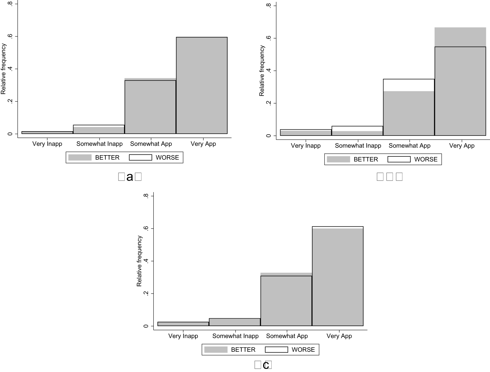
Figure 3 shows the distribution of social appropriateness ratings for the relative performance-based pay criterion among participants who were assigned to the WORSE (white bars) and BETTER treatments (gray bars). The top panels show the distributions in the unincentivized version of the KW task in Wave 1 (top-left,  $\mathrm{N} = 484$) and Wave 2 (top-right,
  $\mathrm{N} = 1,020$), while the bottom panel shows the distributions in the incentivized KW task (
 $\mathrm{N} = 1,008$).
Distribution of Ratings in NoIncentive and Incentive Conditions (a) NO INCENTIVE (Wave 1) (b) NO INCENTIVE (Wave 2) (c) INCENTIVE (Wave 3)

In the NoIncentive condition of Wave 1, we found that the relative performance-based pay criterion is rated as less appropriate by subjects who would be penalized by such pay criterion (WORSE treatment; avg. 0.671, s.d. 0.453) than by those who would be advantaged by it (BETTER treatment; avg. 0.680, s.d. 0.442). The difference goes in the hypothesized direction, but it is small (it corresponds to a Cohen’s d of -0.019 with a 95% confidence interval between -0.198 and 0.159), and is statistically insignificant using a rank-sum test ( $\mathrm{z} = -0.125$; one-tailed p-value
  $ = 0.450$).Footnote 17
As shown in Table 2, with the Wave 1 sample size we are only able to rule out moral hypocrisy effects with an absolute magnitude of Cohen’s d  $\geq$ 0.230. The Wave 2 experiment was run with a larger sample size to rule out effects with an absolute magnitude as small as 0.160. In Wave 2, we found a larger difference in appropriateness ratings between the two treatments. The average appropriateness of the relative performance criterion was 0.605 (s.d. 0.518) in the WORSE treatment, while it was 0.717 (s.d. 0.465) in the BETTER treatment. The corresponding Cohen’s d is −0.228 with a 95% confidence interval between −0.351 and −0.104. We reject the null hypothesis that the two distributions are the same using a rank-sum test (
 $\mathrm{z} = -3.952$; one-tailed p-value
  $ \lt 0.001$).
If we pool the data from Wave 1 and 2 to obtain a more precise estimate of the moral hypocrisy bias, we find that the appropriateness of the relative performance pay criterion is lower in WORSE (avg. 0.626, s.d. 0.499) than in BETTER (avg. 0.705, s.d. 0.457). The corresponding Cohen’s d is −0.165 with a 95% confidence interval between −0.266 and −0.063. We reject the null hypothesis that the two distributions are the same using a rank-sum test ( $\mathrm{z} = -3.343$; one-tailed p-value
  $ \lt 0.001$).Footnote 18
In Wave 3 we ran the WORSE and BETTER treatments in the Incentive condition to assess the persistence of the moral hypocrisy bias in the incentivized KW task. The distributions of ratings are very similar between the WORSE and BETTER treatments. Relative performance-based pay is actually rated slightly more appropriate in the WORSE (avg. 0.674, s.d. 0.476) than BETTER treatment (avg. 0.667, s.d. 0.473). The corresponding Cohen’s d is very small and equal to 0.015 (95% confidence interval between −0.109 and 0.138). We cannot reject the null hypothesis that the two distributions in the Incentivized condition are the same using a rank-sum test ( $\mathrm{z} = 0.364$; one-tailed p-value
 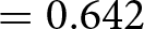 $ = 0.642$).
All results presented above are robust in multivariate regression analysis with controls (performance in the task and socio-demographic characteristics) as well as to the exclusion of subjects who transcribed correctly either 0 or 10 strings and were thus not randomly assigned to treatment (see Appendix I).
As additional analysis, we ran an OLS regression that combines data from the NoIncentive and Incentive conditions and test for the effectiveness of incentives in reducing the moral hypocrisy bias observed in the NoIncentive condition.Footnote 19 We use the following regression specification:
 \begin{equation*}
rating_{i} = \beta_0 + \beta_1 Incentive + \beta_2 WORSE + \beta_3 Incentive\times WORSE + \boldsymbol{X_i} + \epsilon .
\end{equation*}
\begin{equation*}
rating_{i} = \beta_0 + \beta_1 Incentive + \beta_2 WORSE + \beta_3 Incentive\times WORSE + \boldsymbol{X_i} + \epsilon .
\end{equation*} The dependent variable,  $rating_{i}$, is the social appropriateness rating subject
  $i$ assigns to the payment criterion. Incentive is an indicator equal to one if the subject participated in the incentivized version of the KW task and equal to zero for the unincentivized version of the task. WORSE takes value one for subjects assigned to the WORSE treatment, and zero for those assigned to the BETTER treatment. The vector
  $X_i$ includes the socio-demographic controls mentioned earlier plus the number of correctly transcribed strings in the task. Our coefficient of interest is
  $\beta_3$, measuring the effect that monetary incentives in the KW task have on the moral hypocrisy bias relative to the unincentivized task.
Table 3 presents the results in specifications without controls (Model 1) and with controls (Model 2). Both models were run pooling data across Wave 1 and 2 of the NoIncentive condition, which is a slight deviation from our pre-registration (Appendix I replicates the analysis using only Waves 2 and 3 data as pre-registered; results are unchanged). The estimates of the coefficient of the WORSE indicator confirm the result discussed above concerning the existence of a statistically significant moral hypocrisy bias in the NoIncentive condition. In both models, the interaction term Incentive x WORSE is positive and significant at the 5% level, indicating that using monetary incentives in the KW task reduces significantly the moral hypocrisy bias. The coefficient estimates indicate that the bias is completely eliminated by incentives.
Effect of incentives on moral hypocrisy bias
Notes: Robust standard errors in parentheses. Dependent variable in all models: appropriateness rating of the relative performance pay criterion. Controls included in Model (2): number of strings transcribed correctly in the task, gender, age, education, employment status, income, family composition, and country of birth. The drop in number of subjects between Model 1 and 2 is due to missing data in the control variables.
*  $= \mathrm{p} \lt 0.05$, **
  $= \mathrm{p} \lt 0.01$, ***
  $= \mathrm{p} \lt 0.001$, based on one-sided tests.
Overall, these results show that social norm elicitations may be vulnerable to moral hypocrisy biases that arise in situations where subjects perceive a conflict between the prevailing norm in their group and their self-interest. In such cases, our results suggest that monetary incentives can completely eliminate this moral hypocrisy bias.
3.5. Additional results: response quality
In the experiments of Study 2, we collected again data on the time subjects spent in the experiment as well as their responses to the control question probing their understanding of the KW task. Since Study 2 involves both incentivized and unincentivized versions of the KW task, we can use this data to test again for the effect of incentives on response quality, which was the focus of Study 1 (see H1), but with a sample size that is more than twice as large as Study 1.Footnote 20
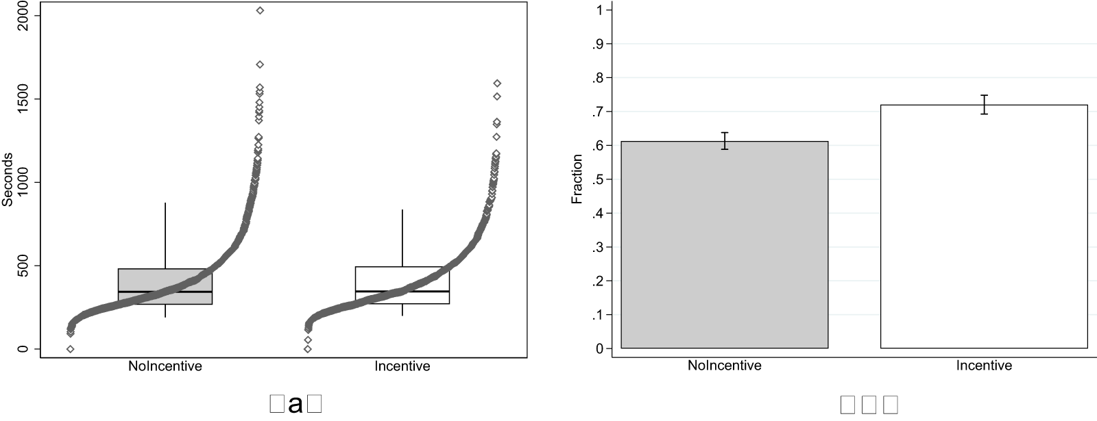
Figure 4 shows the results. We again fail to observe an effect of incentives on time spent in the experiment (left panel). Subjects in the NoIncentive condition spent slightly less time (avg. 410 seconds, s.d. 220) compared to Incentive (avg. 411 seconds, s.d. 203). The effect is however very small, corresponding to a Cohen’s d of 0.007 (95% confidence interval between −0.073 and 0.086) and statistically insignificant on a one-sided t-test ( $\mathrm{t} = 0.160$; one-tailed p-value
 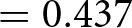 $ = 0.437$, adjusted for MHT using the Benjamini–Hochberg False Discovery Rate method).
Response Quality in Study 2 (a) Task duration (b) % Correct Control Question

As in Study 1, we observe again a positive effect of incentives on the percentage of subjects who answer correctly the control question about the nature of the KW task (right panel of Figure 4). The effect is larger than the one observed in Study 1. In the NoIncentive condition, 61% of subjects selected the correct answer, compared to 72% in the Incentive condition. The increase in the share of correct answers is statistically significant in a test of proportions (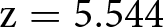 $\mathrm{z} = 5.544$; one-tailed p-value
  $ \lt 0.001$, adjusted for MHT).Footnote 21
4. Study 3: interviewer bias
The main focus of Study 3 was to test whether an interviewer bias influenced responses in social norm elicitation tasks. We pre-registered the experiment on OSF (reproduced in Appendix J), and all hypotheses, exclusion criteria and analyses presented below follow the pre-registration unless explicitly noted. The experiments were programmed using the software SurveyXact and conducted online between December 2024 and January 2025 using participants recruited from Prolific UK (none of these participants took part in any of our other studies).
4.1. Design
Subjects were recruited to take part in a task to evaluate behaviors for a guaranteed participation fee. After indicating their consent to participate in the study, subjects read the instructions of the norm elicitation task (reproduced in Appendix K). They learned that they would be presented with descriptions of behavior in a series of vignettes and that they would be asked to indicate the social appropriateness of the behavior described in each vignette. Subjects were instructed to rate behavior to match the most common rating among other participants taking part in the same experiment. Subjects were not paid to match the modal rating (unincentivized version of the KW task, NoIncentive condition).
After the instructions, subjects answered a control question about the task, similar to the question used in our previous studies. Regardless of their answer, all subjects were then informed of the correct answer and then proceeded to rate behavior in the vignettes.Footnote 22
Subjects then went through either four or three vignettes, depending on the data collection wave (see section 4.3). In each vignette, subjects rated the described behavior using a four-point scale from “Very appropriate” to “Very inappropriate”. After the rating task, we collected the same socio-demographics information as in our previous studies, and the experiment then concluded.
Our treatment manipulation involved displaying a photograph of one of the three researchers on the experiment screens. The photo appeared on the first screen to introduce participants to the study’s contact person and was then displayed on subsequent screens. We randomly varied between subjects whether the researcher shown in the photo was one of the male co-authors (MALE INTERVIEWER treatment) or the female co-author (FEMALE INTERVIEWER treatment).
4.2. Hypotheses and outcome variables
The experiment is designed to test whether norms elicited with an unincentivized version of the Krupka-Weber method are vulnerable to an “interviewer bias”: in settings where respondents perceive a conflict between the social norm within their reference group and the social norm they believe is upheld by the interviewer, they may be inclined to align their evaluations with the interviewer’s perceived norm rather than accurately reporting their group’s actual norm.
In the experiment, we fix the subjects’ reference group by recruiting only participants who report their gender identity as men and informing subjects that in the KW task their objective is to match the ratings of other men recruited in the same experiment.
The treatments vary the observable sex of the researcher as a way to manipulate subjects’ perception of the norm the researcher may hold. In a manipulation check experiment with 198 men recruited from Prolific we find that men and women are indeed perceived to hold different norms in the vignettes included in Study 3 (see Appendix L for details). In all vignettes, the perceived norm among women is less accepting of the described behaviors than the corresponding norm among men. Therefore, if appropriateness ratings in the unincentivized KW task are vulnerable to interviewer bias, we would expect behavior in the vignettes to be rated as less appropriate in the FEMALE INTERVIEWER treatment than in the MALE INTERVIEWER treatment.
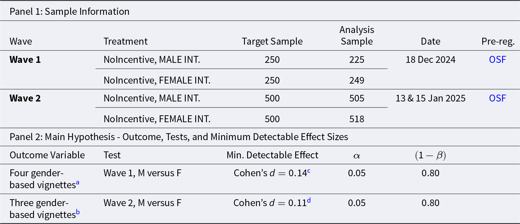
We formally test this hypothesis using regression analysis where we pool the ratings from the vignettes evaluated by a subject and cluster standard errors at the subject-level. We run the following regression model:
 \begin{equation*}
rating_{i, v} = \beta_0 + \beta_1 FEMALE\;\,INTERVIEWER + \boldsymbol{V_v} + \boldsymbol{X_i} + \epsilon .
\end{equation*}
\begin{equation*}
rating_{i, v} = \beta_0 + \beta_1 FEMALE\;\,INTERVIEWER + \boldsymbol{V_v} + \boldsymbol{X_i} + \epsilon .
\end{equation*} where the dependent variable, 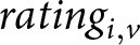 $rating_{i, v}$, measures the social appropriateness rating subject
  $i$ assigns to the behavior described in vignette
  $v$. FEMALE INTERVIEWER is an indicator equal to one if the subject was assigned to the FEMALE INTERVIEWER treatment and equal to zero otherwise. The vector
  $V_v$ includes vignette dummies and the vector
  $X_i$ includes the usual subject-level controls. The coefficient of interest is
  $\beta_1$, which we expect to be negative if appropriateness ratings are vulnerable to interviewer bias.
4.3. Implementation
The study was run across two data collection waves on Prolific UK. Table 4 provides details about sample sizes and power of the analyses for each data collection wave.
Study 3 – sample size and power
a Notes:Career-based sexism, Male breadwinner role, Gendered parenting expectations, and Inappropriate workplace conduct. bCareer-based sexism, Male provider mindset, and Aggressive male fandom. Cohen’s  $d$ refers to the absolute magnitude of the standardized mean difference; that is,
  $|d|$ values are reported without regard to direction. cBased on one-sided t-test with the actual sample size of 474 subjects collected in Wave 1. dBased on one-sided t-test with the target sample size of 500 subjects per treatment.
  $\alpha$ indicates the significance levels used in the tests;
  $(1-\beta)$ indicates the statistical power. See Appendix L for further details.
In Wave 1 we collected 538 observations, of which 482 were unique and complete, and 474 from subjects who moreover identified as men (based on post-experimental questionnaire data) and hence retained for analysis. As main outcome variable, we collected from each subject ratings in four vignettes describing behavior related to career-based sexism, traditional male breadwinner roles, gendered parenting expectations, and potentially inappropriate gendered workplace conduct (see Appendix M for the text of the four vignettes).
As in the case of Study 2, the Wave 1 sample size reflects a partial data collection resulting from our pre-registered sequential sampling strategy (see Appendix N for details on the data collection process). The primary analysis was pre-registered as a difference-in-differences approach aimed at comparing changes in responses between MALE and FEMALE INTERVIEWER treatments across incentivized and unincentivized KW tasks. After the initial data collection, we found the estimated gap between MALE and FEMALE INTERVIEWER treatments too small to support a meaningful diff-in-diff analysis and therefore halted further data collection.
After discontinuing the data collection of Wave 1, we pre-registered a new experiment (Wave 2) that abandoned the diff-in-diff approach as the primary analysis, and instead focused on ruling out small interviewer bias effects in the unincentivized KW task. The Wave 2 experiment was identical to the Wave 1 experiment, with three exceptions. First, we attempted to increase the strength of our treatment manipulation by displaying the researcher’s photos on all screens until the post-experimental questionnaire (in Wave 1 photos were only displayed in the instruction screens and not in the vignette screens). Second, we used three vignettes, of which two were new compared to Wave 1. Specifically, we retained the Wave 1 vignette about career-based sexism, and added two new vignettes describing behavior related to traditional male provider mindset and aggressive male fandom (see Appendix M for the text of the vignettes).Footnote 23 Finally, we paid a slightly larger participation fee in Wave 1 (0.60 GBP) than Wave 2 (0.50 GBP), due to the higher number of vignettes in Wave 1. We collected 1,139 new observations, of which 1,023 were retained for analysis after excluding incomplete and non-unique observations and subjects who did not report their gender as “man” in the post-experimental questionnaire.Footnote 24
4.4. Results
Figure 5 shows the distribution of appropriateness ratings in the seven vignettes used in Waves 1 and 2.Footnote 25 The gray bars show the distributions in the MALE INTERVIEWER treatment and the white bars those in the FEMALE INTERVIEWER treatment.
Distribution of ratings in study 3 vignettes (a) Gend. parenting expect. (W1) (b) Career-based sexism (W1), (c) Inapp. workplace conduct (W1), (d) Male breadwinner role (W1), (e) Career-based sexism (W2), (f) Male provider mindset (W2), (g) Aggressive male fandom (W2)
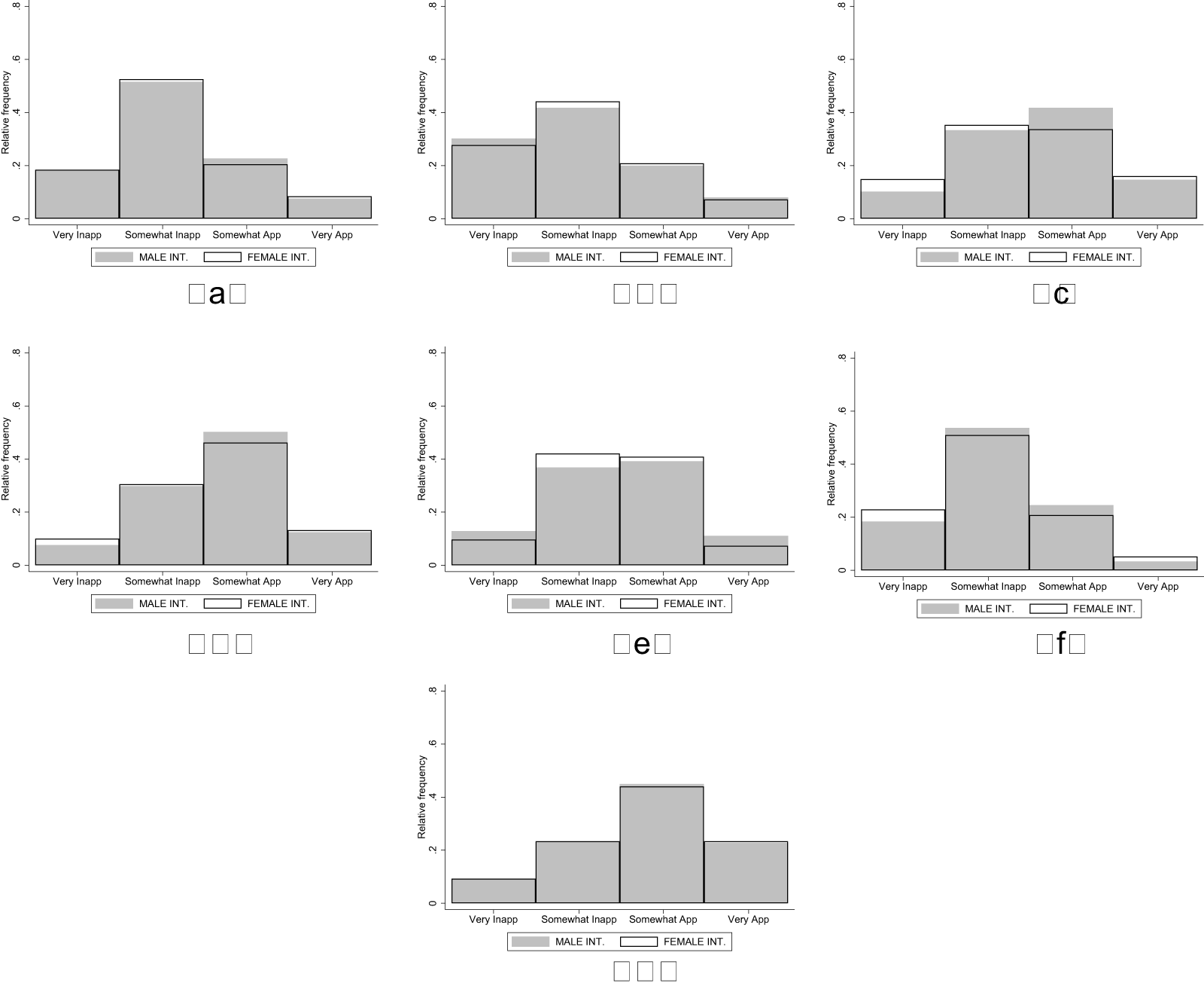
There are only very small differences in the rating distributions across treatments in all vignettes. Averaging across the seven vignettes, the observed Cohen’s d is very small and equal to −0.033 (−0.038 across the four vignettes of Wave 1 and −0.026 across the three vignettes of Wave 2). Formal analysis using the regression model detailed above is reported in Table 5 and confirms that the appropriateness ratings are not significantly different across treatments in Wave 1, Wave 2, or Wave 1 and Wave 2 combined. Results are robust to the model specification (ordered logit instead of OLS) and hold when we conduct separate analyses for each vignette (see Appendix O for details). The results are also robust to controlling for, or excluding, subjects affected by the programming error described in footnote 22 (see Appendix O). Overall, in our setting, the KW task seems robust to interviewer bias even in the absence of monetary incentives.
Interviewer bias in the unincentivized kw task - OLS regressions
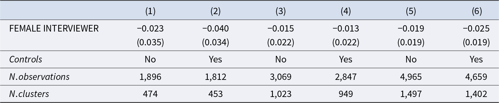
Notes: Robust standard errors clustered at the subject level in parentheses. Dependent variable in all models: appropriateness rating of the behavior described in the vignettes. Models (1) and (2) use Wave 1 data. Models (3) and (4) use Wave 2 data. Models (5) and (6) use pooled data from Wave 1 and Wave 2. All models include vignette dummies. Controls further included in Model (2), (4) and (6): age, education, employment status, income, family composition and country of birth. The drop in number of subjects in the models with controls is due to missing data in the control variables. *  $= \mathrm{p} \lt 0.05$, **
  $= \mathrm{p} \lt 0.01$, ***
  $= \mathrm{p} \lt 0.001$, based on one-sided tests.
5. Conclusions
Should subjects be provided with incentives to match other participants’ responses in the Krupka-Weber norm elicitation task? Previous evidence from distributional games (Veselý, Reference Veselý2015; König-Kersting, Reference König-Kersting2024; Huffman et al., Reference Huffman, Kohno, Madies, Vogrinec, Wang and Yagnaraman2024) and perceived norms of political ideology (Groenendyk et al., Reference Groenendyk, Kimbrough and Pickup2023) suggests incentives have a neutral impact on responses, as elicited norms have been found not to differ significantly between elicitations with and without incentives. While previous studies have mostly focused on examining the role of incentives in reducing response noise and improving response quality, this paper extends the analysis to cover a wide range of channels through which incentives may affect responses in KW tasks.
In line with previous results, we find only small improvements in terms of response quality between versions of the KW task with and without monetary incentives. The largest effect – detected in one of the two studies where it could be tested – is that incentives seem to improve subjects’ understanding of the KW task. Specifically, incentives help participants grasp that the task requires them to focus on their perception of what others recognize as appropriate or inappropriate, rather than on their own personal assessment. Given that this is a central feature of the KW task (and of norm-elicitation tasks, more generally) and that a surprisingly small share of subjects seem to actually grasp it (between 54% and 62% across all our studies without incentives), this may be a non-negligible advantage of using monetary incentives in the context of norm elicitation tasks. However, the actual improvement in understanding when incentives are used is relatively small (between 4 and 11 percentage points across our studies). Huffman et al. Reference Huffman, Kohno, Madies, Vogrinec, Wang and Yagnaraman2024 and König-Kersting Reference König-Kersting(2024) report comparably small effects of incentives on task comprehension in their experiments.
The result may appear surprising in face of the long-standing debate in the experimental economics literature about the role of incentives in overcoming decision errors and reducing response noise (see, e.g.,Fouraker & Siegel, Reference Fouraker and Siegel1963; Harrison, Reference Harrison1989; Smith & Walker, Reference Smith and Walker1993a; Smith & Walker, Reference Smith and Walker1993b). In their seminal review of the role financial incentives in experiments, Camerer and Hogarth (Reference Camerer and Hogarth1999) found that incentives primarily affect participants’ decisions when performance can be improved through increased effort. By contrast, incentives tend to have limited effects in tasks that are either very easy (due to ceiling effects) or very difficult (due to floor effects), where performance is constrained regardless of effort. The weak effects of incentives on response quality in our experiments may reflect a similar constraint: a lack of knowledge about norms is not something that incentives can easily overcome. If norms function as focal points that naturally come to mind and help coordinate judgment and behavior, it is unclear whether offering incentives would make participants more likely to derive the relevant norm from context or enable them to do so more effectively.Footnote 26
Also in line with previous results, we do not find support for the argument that monetary incentives may distort responses by encouraging participants to coordinate their ratings using focal points unrelated to the social norm. This focal point distortion has been tested in related papers by Fallucchi and Nosenzo Reference Fallucchi and Nosenzo(2022) and Aycinena et al. (Reference Aycinena, Bogliacino and Kimbrough2024c) that did not find any evidence for it. We provide further corroborating evidence that this distortionary effect seems negligible in incentivized versions of the KW task. Similarly, we do not find support for the previously untested conjecture that incentives may distort normative judgments towards materialistic values.
We also study the role of response biases in the KW task. We do not find evidence of interviewer bias in an unincentivized version of the task. This result chimes in with Aycinena et al. Reference Aycinena, Bogliacino and Kimbrough(2024b), who study whether the norm elicitation approach suggested by Bicchieri and Xiao Reference Bicchieri and Xiao(2009) is vulnerable to social desirability bias. In Bicchieri and Xiao Reference Bicchieri and Xiao(2009), norms are elicited using a two-step procedure, where in a first step subjects are asked to report unincentivized personal judgments about the appropriateness of behavior, and in a second step (which is used to elicit the social norm) subjects report their guess about the modal response in the first step. The lack of incentives in the first step of the procedure raises concerns about the vulnerability of the method to response biases such as social desirable responding (Görges & Nosenzo, Reference Görges and Nosenzo2020; Aycinena et al., Reference Aycinena, Bogliacino and Kimbrough2024b). However, Aycinena et al. Reference Aycinena, Bogliacino and Kimbrough(2024b) find weak evidence of social desirable responding in their study.
Our study provides instead support to the notion that subjects may distort responses to portray behavior and/or outcomes that are materially advantageous to them as more appropriate. This bias, which we referred to as “moral hypocrisy” following the terminology of Rustichini and Villeval (Reference Rustichini and Villeval2014), has been documented in previous opinion tasks, and we also find evidence of it in an unincentivized version of the KW task. However, when incentives are introduced, the bias disappears. Thus, incentives seem effective in addressing response biases driven by self-serving rationalizations.
This result is in line with Amasino et al. Reference Amasino, Pace and van der Weele(2023) who study an analogous self-serving bias in norms related to redistribution choices. They measure both personal norms (unincentivized assessments of the appropriateness of various redistribution options) and social norms using the KW task. They find evidence of self-serving responses in the personal norms, but not in the norms elicited with the KW method. Although incentivization is not the only difference between personal and social norms, their evidence aligns with ours in suggesting that incentives may be effective in correcting this type of distortion in the elicitation of normative judgments.
To circle back to our initial question, should a researcher provide incentives for subjects to match other participants’ responses in the Krupka-Weber norm elicitation task? Based on the joint results from our studies and previous literature, we have four suggestions for researchers interested in using norm-elicitation methods:
• If the primary concern is response quality (time spent in the task, attention to detail, understanding of the task), the benefits of using incentives may not outweigh the costs – at least not in an online setting such as that where we ran our studies. However, given that understanding of the task is worryingly low (as also noted in previous studies), we recommend researchers include an explicit control question to assess comprehension and consider excluding subjects who answer it incorrectly.
• Incentives are particularly recommended when a researcher is concerned about distortions stemming from response biases. These biases may arise for different reasons in various settings, and our study suggests that not all biases necessarily distort responses in the KW task when incentives are absent. Nonetheless, incentives seem effective at eliminating such biases, should they occur.
• Moral hypocrisy biases may be particularly likely to arise in settings where subjects report their perceptions of the appropriateness of actions that were available to them in an earlier stage of the experiment. In such cases, we recommend using incentives. For the same reason, the use of methods that partially rely on unincentivized responses, such as the approach used by Bicchieri and Xiao Reference Bicchieri and Xiao(2009), may not be advisable in these settings.
• Although focal point distortion remains a theoretical possibility in the KW task, the accumulated evidence offers no empirical support for it. Therefore, we do not consider it a compelling argument against the use of incentives in KW tasks.
Acknowledgements
This work was funded by the Aarhus University Research Foundation (AUFF Starting Grant 36835). The project underwent research ethics review and was approved by the Committee for the Integrity and Ethics of Research of the University of Bergamo on December 13, 2024. Ref: 2024_12_06. The replication material for the study is available at https://osf.io/fvt93. We thank the Editors and two anonymous referees for helpful comments, and Thais Cardarelli, Alexander Koch, Zhenxun Liu and Julia Nafziger for useful discussions.


 Open access