

Introduction
Groningen field
The Groningen field is the largest onshore gas accumulation in Europe (~2900×109Nm3 gas initially in place) (Grötsch et al., Reference Grötsch, Sluijk, van Ojik, de Keijzer, Graaf and Steenbrink2011; Figs 1 and 2). The gas-bearing section comprises both aeolian and fluvial-deltaic sandstones of the Upper Rotliegend Group (Permian) and fluvial sandstones of the Limburg Group (Upper Carboniferous) intercalated by shale layers of the Ten Boer Claystone and Ameland Claystone (de Jager & Visser, Reference de Jager and Visser2017). The field is sourced from extensive Westphalian coals and Namurian carbonaceous shales directly below the field (e.g. Gerling et al., Reference Gerling, Geluk, Kockel, Lokhorst, Lott, Nicholson, Fleet and Boldy1999; Grötsch et al., Reference Grötsch, Sluijk, van Ojik, de Keijzer, Graaf and Steenbrink2011). Thick Zechstein evaporites act as a seal. Continuous production since 1963 has led to induced seismicity starting in the early 1990s. The first earthquake in the field was recorded in 1991 (M L 2.4) after 1272×109Nm3 of gas had been produced (Hettema et al., Reference Hettema, Jaarsma, Schroot and van Yperen2017). From 2003 onwards, the number of earthquakes and their magnitudes increased. The largest earthquake (M L 3.6) was recorded in 2012 near Huizinge and caused the most damage to date (e.g. Van Thienen-Visser & Breunese, Reference Van Thienen-Visser and Breunese2015), possibly as a result of its uncommon seismological characteristics, as described in Dost & Kraaijpoel (Reference Dost and Kraaijpoel2013). Production measures aimed at lowering the level of seismicity have been implemented since 2014. These measures were imposed in a few steps after 2014, comprising reduction of the maximum allowed annual production and avoidance of production fluctuations in time and space.
Top Rotliegend depth map with Groningen field outline in red (NAM, Reference van Elk and Doornhof2016a). Black lines indicate current reservoir fault model (NAM, Reference van Elk and Doornhof2016a). Blue circles indicate seismic events from 1991 through 2016 (M L≥1.3) (KNMI, 2017; Spetzler & Dost, Reference Spetzler and Dost2017).

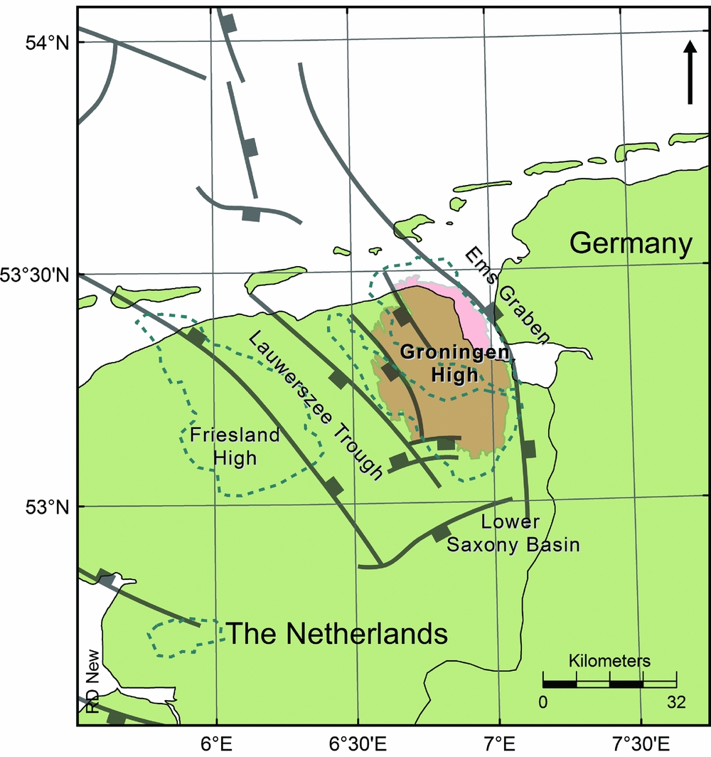
Regional setting and structural elements of the Groningen region. The Groningen gas field is indicated in red; green dashed lines indicate the Dinantian carbonate platforms (outlines of platforms from Hoornveld, Reference Hoornveld2013).
Roles of faults
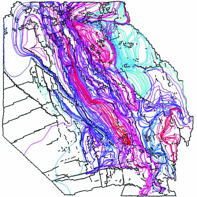
Faults play an important role during the production lifetime of the Groningen field as they subdivide regions in the field. Fault properties such as transmissibility and slip resistance may vary throughout the field and even along a fault, as a result of differences in the amount and orientations of stress and strain, the throw and differences in local diagenesis (e.g. Knipe et al., Reference Knipe, Jones, Fisher, Jones, Fisher and Knipe1998; Ligtenberg et al., Reference Ligtenberg, Okkerman and de Keijzer2011). On a geological timescale, large regions can be identified in the Groningen field that display different initial free water levels (NAM, Reference van Elk and Doornhof2016a) suggesting that faults or fault zones acted as barriers to cross-fault communication in the past and may still do so. Differences in capillary pressure could also play a role. In the history-matching process of the Groningen field, special attention was paid to the calibration of fault transmissibilities. Assisted history matching was used to find different realisations that match gas production, reservoir pressures and rising water tables (NAM, Reference van Elk and Doornhof2016a). An example of preferred flow paths through the Groningen reservoir is shown in the streamline map (Fig. 10, further below). This is a visualisation of the shortest route for a gas molecule to flow through the reservoir model to a nearby well at a moment in time. This route is mostly determined by the modelled permeability and fault transmissibility. The picture indicates that most production clusters have a specific area from which the (bulk of the) production comes (so-called drainage areas). More faults and realistic geometries can be included in the reservoir model and could help understanding the flow of gas from one block to another, across the faults and fault zones.
The induced seismicity in the Groningen field is related to pre-existing faults at reservoir level (e.g. Dost et al., Reference Dost, Goutbeek, van Eck and Kraaijpoel2012; Nepveu et al., Reference Nepveu, Van Thienen-Visser and Sijacic2016). Faults are local weak zones in the rocks and are used to accommodate stress by pressure differences in relation to the later stage of production with significant depletion. Slip of these faults is expected when shear traction is sufficient to overcome frictional resistance (see e.g. Dost et al., Reference Dost, Goutbeek, van Eck and Kraaijpoel2012; Bourne et al., Reference Bourne, Oates, van Elk and Doornhof2014). The objective is to understand which (parts of the) faults are more susceptible to seismicity; these insights could be used to optimise the production strategy and minimise seismic risk.
It is clear that faults play a major role in the Groningen field, both in the production of gas and in the associated seismicity, and hence that a detailed and realistic fault model is important. Deterministic, probabilistic and empirical models have been developed in recent years to predict seismicity as a function of production and local subsurface conditions in the Groningen field. The deterministic and probabilistic models often take into account faults at reservoir level. For instance, in geomechanical modelling of seismogenic behaviour along fault planes at a local scale (e.g. Wentinck, Reference Wentinck2015), detailed fault shapes are crucial. Bourne et al. (Reference Bourne and Oates2015a,b) developed probabilistic models to predict seismicity in terms of numbers, location and magnitude as a function of production. Bourne et al. (Reference Bourne and Oates2015a) concluded that the relationship between earthquake hypocentres and mapped faults is statistically significant but rather uncertain due to the large uncertainty in hypocentral locations. They did not find evidence that faults with any particular azimuth are more prone to seismicity than others.
Obtaining better geometric descriptions in terms of positioning and fault throw offsets and using more detailed fault planes in the probabilistic and deterministic studies as described above will lead to more robust models with larger predictive power. This paper demonstrates that the definition of faults in the Groningen field can be improved using 3D seismic attributes and that detailed 3D fault planes can be extracted from the seismic data.
Regional tectonic history of the Groningen area
The Groningen field is located on the Groningen High. This structural high is bounded by the Lauwerszee Trough towards the west, the Ems Graben in the east and the Lower Saxony basin in the south (Fig. 2). Two large Early Carboniferous (Dinantian) carbonate platforms are present here (see e.g. Kombrink, Reference Kombrink2008; Van Hulten, Reference Van Hulten2012; Hoornveld, Reference Hoornveld2013) (Fig. 2). Similar platforms are present to the west (Hoornveld, Reference Hoornveld2013). Three major tectonic events affected the region: (1) the Carboniferous Variscan Orogeny (compressional phase), (2) the Mesozoic break-up of Pangaea and related opening of the Atlantic (extensional phase), and (3) the Late Cretaceous to Early Tertiary deformation (compressional phase) (Ligtenberg et al., Reference Ligtenberg, Okkerman and de Keijzer2011 and references therein). These tectonic events had different main stress orientations, resulting in oblique stress on the various existing fault systems through tectonic history.
The Variscan Orogeny started in the Early Carboniferous and ended during the Late Westphalian and had an approximately N–S compressional direction. The E–W striking faults are often associated with the Variscan compressional event (Ligtenberg et al., Reference Ligtenberg, Okkerman and de Keijzer2011 and references therein). At the end of the Carboniferous the area was subjected to post-orogenic tectonism associated with oblique-slip faulting and thermal uplift. The oblique-slip faulting resulted in the development of large NE–SW and NW–SE conjugate fault systems. The presence of these two fault trends at the Rotliegend level clearly indicates that many of the older faults (in deeper strata) have been reactivated during different subsequent tectonic events. The second tectonic phase (consisting of multiple phases) was extensional (NE–SW) and started in the Early Triassic up to the Early Cretaceous. The Late Jurassic Atlantic opening and North Sea (failed) rifting is important for the Groningen region; the Lauwerszee Trough, Ems Graben and Rodewolt fault zone that cross-cuts the Groningen field were developed, reactivating the pre-existing structural grain. The last major stage of deformation took place from the Late Cretaceous to the Early Tertiary (Alpine inversion). The direction of compressional stress was approximately N–S (Ligtenberg et al., Reference Ligtenberg, Okkerman and de Keijzer2011). Again, during these latter tectonic phases pre-existing older faults have been reactivated, as is observed elsewhere in the basin (e.g. Schroot & de Haan, Reference Schroot, de Haan and Nieuwland2003). Expressions of the Alpine inversion event are the local presence of overthrusts and the occurrence of pop-ups along major NW–SE fault trends (Ligtenberg et al., Reference Ligtenberg, Okkerman and de Keijzer2011).
Fault identification and fault plane extraction using seismic attributes
It is well known that faults which can be imaged and interpreted on seismic as single, rather straight surfaces could in reality represent more complex zones which may consist of a fault core (with sharp fault surfaces, breccia, fault gouge) and a fault damage zone around this. Many of these features, obviously, have dimensions below seismic resolution (e.g. Knipe et al., Reference Knipe, Jones, Fisher, Jones, Fisher and Knipe1998).
In conventional seismic interpretation, faults are interpreted on (vertical) seismic sections by visual inspection and manual picking. The faults are defined by fault sticks which can then, after interpolation, be input for a structural model. This workflow had been applied to the Groningen field, where 627 faults with an expression at reservoir level were manually picked on pre-stack depth migration (PreSDM) seismic data (NAM, 2015).
Faults appear as discontinuities in seismic datasets. However, faults with relatively small or no throw will hardly or not be visible. Still such faults may be important, as, for example, the remaining throw is the net result of successive tectonic phases. Various structural seismic attributes can be used to delineate faults that would be difficult to map in a conventional way using standard amplitude data. These attributes are derivatives of the basic seismic measurements (time, amplitude, frequency and attenuation), calculating and extracting spatial discontinuities at a smaller scale. The attributes will allow for more detailed characterisation of fault delineations and geometries compared to manually interpreted fault planes (e.g. Chopra & Marfurt, Reference Chopra and Marfurt2008).
The seismic dataset used in our workflow is a 3D seismic volume which covers the entire Groningen field. This dataset comprises a number of surveys acquired in the 1980s and 1990s. A major reprocessing and depth-imaging project in 2015 resulted in various PreSDM volumes in time and depth domain. Manual fault interpretation of deep continuous faults (from Rotliegend into Upper and Lower Carboniferous strata) in the Loppersum area using the reverse time migrated (RTM) seismic data was performed and is described in this paper.
In this section the workflow of fault characterisation and fault plane extraction, applied to the Groningen field, is described. The workflow consists of two steps: the first step starts with conditioning the seismic input data, followed by iterative attribute extractions; the second step is the extraction of fault planes (‘geobodies’) from the attribute cube of the first step.
First, a structurally oriented smoothing filter was applied (Daber & Aqrawi, Reference Daber and Aqrawi2011) to attenuate random noise and to enhance the discontinuities in the seismic volume. Subsequently, a variance (edge) cube (Van Bemmel & Pepper, Reference Van Bemmel and Pepper2000) was generated from the smoothed cube, to capture the spatial discontinuity of the seismic dataset. Petrel Ant Tracking (®Schlumberger) was then applied on the variance cube in three iterations with so-called ‘aggressive’, ‘passive’ and again ‘passive’ settings. In these iterations, a number of parameters were set, switching between stronger and weaker amplification of discontinuities for the process. The parameter settings determine the number and detail of discontinuities (faults) which will be derived from the seismic data. A dip inclination filter was applied to disregard discontinuities (faults) with less than 60°. Ant tracking is a technology that performs edge enhancement to identify faults and other linear anomalies within the input seismic volume. Swarm intelligence concepts are used to introduce a high number of ‘ants’ into the volume and evaluate the collective behaviour of the swarm. Various settings are set to distribute, guide and limit the ‘ants’ in the search for larger or smaller, subtle, discontinuities in the volume (Pedersen et al., Reference Pedersen, Randen, Sønneland and Øyvind2002; Daber & Aqrawi, Reference Daber and Aqrawi2011). The ant tracking algorithm draws an analogy from ants finding the shortest distance between their nest and their food source communicating by pheromones, which attracts other ants. Ants following the shortest path will reach their destination earlier and influence other ants by pheromones to take the same path. The shorter path will be more and more marked by pheromones (e.g. Chopra & Marfurt, Reference Chopra and Marfurt2008).
In the second part of the workflow, fault geobodies were extracted from the ant tracking volume using the opacity filter within the Petrel Geobody Interpretation process. The opacity filter was applied to filter out lower-confidence ant tracks. Only the highest level of ant tracking attribute values are included in the geobody extraction. These geobodies represent 3D fault planes which can be exported for input into geomechanical modelling tools.
Results of Groningen fault identification
Improved definition of faults
Figure 3A shows the final ant tracking attribute extracted at the top Rotliegend horizon in depth. Most of the extracted ants at top Rotliegend correspond to faults visible in seismic sections (see also Fig. 6B). The manually interpreted faults used for the reservoir model of the field (NAM, Reference van Elk and Doornhof2016a) are shown in red in Figure 3B. Most of the main faults from the reservoir fault model in red match the faults identified by the ant tracking. Obviously, ant tracking reveals many more faults in the 3D seismic data than are present in the reservoir fault model (NAM, Reference van Elk and Doornhof2016a). Also a number of faults in the reservoir model (NAM, Reference van Elk and Doornhof2016a) differ from the ant tracks. This discrepancy is especially clear in Figure 4 which shows a close-up of the area around the municipality of Loppersum. This area is the region with the highest seismic event density in the Groningen field. Fault definition based on seismic attributes provides an improved representation of fault patterns and whether individual faults connect or not.
(A, B) Ant tracking attribute extracted from NAM's 2015 Groningen PreSDM cube. Extraction along top Rotliegend horizon in depth domain. The Groningen field is outlined in blue. (B) Red lines indicate the reservoir fault model (NAM, Reference van Elk and Doornhof2016a). The ant tracking attribute indicates the presence of many more faults.

Ant tracking attribute extracted at top Rotliegend (depth) in the Loppersum area. Top Rotliegend depth map underlies the ant tracking extraction. Faults (NAM, Reference van Elk and Doornhof2016a) are indicated in red. Circles indicate the KNMI earthquake dataset (M L≥1.3) (KNMI, 2017) including 87 revised hypocentres from Spetzler & Dost (Reference Spetzler and Dost2017) and the updated Huizinge ML 3.6 hypocentre (Dost & Kraaijpoel, Reference Dost and Kraaijpoel2013). Black line indicates seismic section (Fig. 6B).

Ant tracking can also help to define the vertical extent of faults into the Carboniferous. The seismic section in Figure 5A shows a number of manually interpreted faults extending into Upper Carboniferous strata. Many faults extend to the Lower Carboniferous Limestone Group of the Zeeland Formation (Dinantian carbonates), and a number of these faults might even extend into the Dinantian carbonate platform. The seismic section and map of the top Dinantian carbonates suggests a higher density of (conjugate) faults at the slope of the Dinantian carbonate platform (see also Fig. 5B).
(A) Seismic depth section showing Groningen reservoir faults in black (NAM, Reference van Elk and Doornhof2016a). A number of these faults extend into underlying Carboniferous strata (dark grey dashed lines). The bounding fault of the Groningen field terminates at the edge of the Dinantian carbonate platform). Three times vertical exaggeration was applied to improve visualisation; note that this affects the dip imaging of the faults (faults appear steeper). Seismic shown is 2015 PreSDM RTM volume. (B) Map of top Dinantian carbonates (Hoornveld, Reference Hoornveld2013; Langemeijer, Reference Langemeijer2017). Groningen reservoir fault model is indicated in black (NAM, Reference van Elk and Doornhof2016a). Location of seismic section (Fig. 5A) is indicated by dark red line.

On top of the Rotliegend reservoir, basal Zechstein carbonates and ductile Zechstein evaporites are deposited. One would expect no vertical extension of the fault planes above the basal Zechstein carbonates, but ant tracking does show discontinuities within the ductile Zechstein salts (Fig. 6B). Most likely these discontinuities are related to the Zechstein carbonate rafts within the salt. These rafts show strong amplitudes affecting the underlying seismic image of the salt and hence affect the ant tracking within the salt.
(A) Ant tracking attribute extracted at top Rotliegend (depth) in the Loppersum area. Reservoir faults (NAM, Reference van Elk and Doornhof2016a) in red. Black open circle indicates the Huizinge M L 3.6 hypocentre (KNMI, 2017). Red circle indicates revised hypocentral location of Huizinge M L 3.6 earthquake (Dost & Kraaijpoel, Reference Dost and Kraaijpoel2013). (B) Seismic section displaying the ant tracking attribute and the reflectivity data (for location see Fig. 4). The red dot indicates the updated Huizinge M L 3.6 hypocentre (Dost & Kraaijpoel, Reference Dost and Kraaijpoel2013) (3× vertical exaggeration was applied for visualisation purposes).

Improved hypocentre–faults relationship possible: fault at hypocentre Huizinge ML 3.6 earthquake located
The hypocentre of the largest recorded earthquake in the Groningen area has been refined using a local velocity model and using additional data from the local acceleration network (Dost & Kraaijpoel, Reference Dost and Kraaijpoel2013). Figure 6A shows both the original (in open black circle) and refined (in red) hypocentre location of the Huizinge M L 3.6 earthquake. The updated location shifted 500m to the west relative to the original location. The currently used fault model (NAM, Reference van Elk and Doornhof2016a) does not show a mapped fault at this updated hypocentre location. The ant tracking attribute volume, however, does indicate the presence of a fault at this location, suggesting we have identified the fault associated with the Huizinge M L 3.6 event. It must be noted that the uncertainty in hypocentre locations is generally 500m. Dost and Kraaijpoel (Reference Dost and Kraaijpoel2013) also describe a normal fault with a strike of 320° as focal mechanism of this particular earthquake. This strike corresponds to the strike of the fault identified by ant tracking at this hypocentre location. The seismic section confirms a seismic discontinuity and presence of fault at this preferred location; the throw of this fault is relatively small (Fig. 6B).
Detailed fault geometries based on seismic attributes
Geobodies extracted from the ant tracking attribute show more detailed fault geometry than manually interpreted faults and demonstrate the large variation in shape along the fault planes (Fig. 7). Variations in dip, azimuth, roughness etc. can be calculated for these fault planes, improving the input parameters in geomechanical analyses. The geobody faults also show the presence of both simple single fault zones and the typical ‘en-echelon’ type of fault zones (Figs 7, 8).
3D image of the NW–SE extracted geobodies from the ant tracking attribute revealing both simple single fault zones and typical ‘en-echelon’ type of fault zones (3× vertical exaggeration was applied to improve the visualisation).

Map view of the NW–SE extracted geobodies from the ant tracking attribute revealing both the simple single fault zones and typical ‘en-echelon’ type of fault zones. The coloured lines indicate the NAM reservoir fault model (NAM, Reference van Elk and Doornhof2016a). As a NW–SE filtering was applied in the extraction process of the geobodies, only geobody faults in this direction are shown on the map.

Discussion
As explained in the introduction, faults play various important roles in the Groningen field production and the associated induced seismicity. Probabilistic and deterministic modelling require a fault model which is as detailed and as realistic as possible. The available Groningen fault model consists of 627 faults (NAM, Reference van Elk and Doornhof2016a) and was originally constructed to assist the reservoir modelling and production history match analyses. In general, reservoir models are upscaled to include faults that matter in the dynamic behaviour of the field during production. This is different from a fault model that is generated to analyse faults in relation to seismicity.
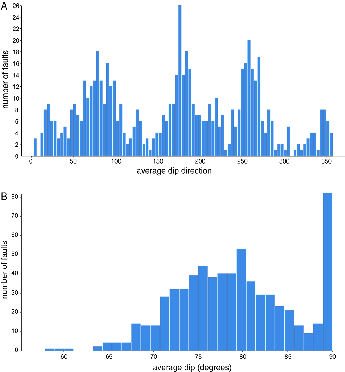
Figure 1 shows the Groningen fault model (NAM, Reference van Elk and Doornhof2016a), indicating various fault trends in different regions of the Groningen field. Figure 5A and B suggest that the deeper geology (Groningen High and related Dinantian carbonate platforms) influences the structural domains identified within the Groningen field. The seismic section and map of the top Dinantian carbonates show a higher density of (conjugate) faults in the Rotliegend, Westphalian and Namurian strata above the slope of the Dinantian carbonate platform (Fig. 5A, B). The most obvious Rotliegend fault trend in the Groningen field is the NW–SE fault trend. Towards the south, faults parallel to the W–E graben that separates the Groningen High from the Lower Saxony Basin become more prominent. These trends also emerge from the calculated average dip directions of the reservoir fault model from NAM (Reference van Elk and Doornhof2016a) (Fig. 9A). Average dip values of the Groningen faults (NAM, Reference van Elk and Doornhof2016a) are described in Figure 9B showing a distribution of 65–90°. In fact, the vertical 90° dip values must be excluded as (most of) these relate to faults where no dip was assigned based on seismic interpretation (NAM, pers. comm., 2016). TNO already compared the fault model to an ant tracking depth slice in 2013 (TNO, 2013) and concluded that the modelled faults match the ant tracking but that many more small faults are present in the field.
(A) Four dominant average dip directions of the Groningen reservoir fault model (NAM, Reference van Elk and Doornhof2016a). (B) Average fault dip of the faults in the Groningen reservoir fault model (NAM, Reference van Elk and Doornhof2016a). Note that faults with a dip of 90° must be excluded from the dataset as these faults have been assigned a vertical geometry (instead of geometry based on seismic interpretation) (NAM, pers. comm., 2016).
The workflow described in this paper and the use of the latest reprocessed and depth-imaged 3D seismic dataset improves the fault identification to such a level that more detailed and accurate fault mapping is possible and detailed fault geometries can be extracted. Figure 3A and B show that the ant tracking extraction at top Rotliegend results in a detailed fault map. The faults from the reservoir fault model (NAM, Reference van Elk and Doornhof2016a) match the faults identified by the ant tracking. Seismic sections show that most of the additional faults identified by ant tracking are also visible in seismic sections. The ant tracking faults display similar strike variations as the general Rotliegend fault trends described above.
The ant tracking process will track many discontinuities visible in the seismic dataset. This may cause difficulties distinguishing between low-angle faults and other features with low angles such as dipping beds and amplitude anomalies. The faults in the Groningen field are relatively steep (Fig. 9B), supporting the choice to filter out features with a dip below 60°. The workflow that includes structural smoothing in addition to the three successive ant tracking steps reduces already much of the incoherent noise which may be present in seismic datasets. Acquisition imprints should also always be considered. In our case, the acquisition imprints which are still present at 100m depth are not visible at reservoir level. The very bright amplitudes of the Zechstein carbonate rafts do influence the seismic imaging of especially the salt underneath and might have some effect in the ant tracking within the salt (Fig. 6B). Some of the edges of rafts do seem to correspond to major faults at Rotliegend level. One should always review the ant tracking results (or, in fact, any seismic attribute) with geology in mind, being careful not to over-interpret the results.
Implementing a very detailed fault model in static and dynamic models of the Groningen field will remain challenging in the near future due to limitations in modelling resolution and computing power. However, including a more detailed fault model may have a considerable impact on the modelling results. First, the flow paths through the reservoir (Fig. 10) are likely to change since faults may not be connected, leading to flow of gas between fault blocks and because fault transmissibility may vary along the length of a fault. Second, the number of faults may increase, requiring recalibrating the transmissibilities of faults or fault zones. The above insights will improve our understanding of how depletion and pressure drop will develop as a function of variations in production from the different production clusters. Improving our understanding of the dynamic behaviour of the field can assist in optimising production measures that minimise seismic risk.
Streamline map (from fig. 4.7 in NAM, Reference van Elk and Doornhof2016a) indicating direction of gas flow coloured by arriving producer well. Streamlines seem to be preferentially oriented along a NW–SE trend and are controlled by fault transmissibility factors.
Bourne et al. (Reference Bourne and Oates2015a) compared the distribution of earthquake hypocentres and mapped faults, using the M≥1.5 events from April 1995 till 30 October 2012. They concluded that the relationship is statistically significant but rather uncertain because the random measurement errors in hypocentral locations are large relative to typical distances between mapped faults (in the order of 500m). They did not find evidence that faults of any particular strike experience preferential seismicity. These analyses would benefit from (1) a decrease in measurement error in the hypocentre location and (2) a more detailed fault model. Decreasing the uncertainty of the hypocentre location can be achieved in various ways. Improvements have already been achieved by the extension of the seismological monitoring network in the Groningen area over the past years (e.g. Spetzler & Dost, in press). Recent installation of deep geophones in the Zeerijp and Stedum wells to monitor (micro-) seismicity in the Loppersum area has resulted in additional data which are also valuable for hypocentre–fault relationship analyses in this region. The implementation of new algorithms in the inversion of the seismological data can improve the depth resolution to 100–200m (Spetzler & Dost, in press). A detailed discussion on this is beyond the scope of this paper.
A more detailed fault dataset can be built when following the workflow described in this paper. Statistical analyses should be (re-)done with such a detailed fault dataset, possibly leading to more robust relationships and providing new insights into the fault dip, azimuth or other fault characteristics which may be preferential to slip. This should be combined with geomechanical studies using the same, detailed fault geometries as input, to confirm statistical findings. In addition, a more detailed fault model will help in analysing recent developments of seismicity in the field, as part of the Groningen seismicity monitoring programme (NAM, 2016c). Figure 6B shows that the fault related to the Huizinge M L 3.6 event has a relatively small throw. This also suggests that the faults now showing a minor throw may be important in seismicity studies and that for hypocentre–fault correlation studies the fault model needs a significant level of detail. In view of the fact that many of the faults have been reactivated a few times throughout geological history, faults with small offset could also be relevant.
Ant tracking also helps to define the vertical extent of faults into the Carboniferous. From Figures 5A and 6B it is clear that a number of faults extend from the Rotliegend reservoir downward into Carboniferous strata. Using the correct shape and vertical extent of faults is important in assessments of which magnitudes of earthquakes may occur in the Groningen field (NAM, Reference van Elk and Doornhof2016b). Geobodies extracted from the ant tracking attribute show more detailed fault geometry. They are currently being used in the geomechanical modelling of seismogenic behaviour (e.g. Wentinck, Reference Wentinck2015, Reference Wentinck2017).
Conclusions
This paper shows that the use of seismic attributes can significantly improve the fault definition in the Groningen area, while geobodies extracted from these seismic attributes provide detailed fault geometries. The detailed fault realisation will help to establish hypocentre–fault relationships, and increase our understanding of the dynamic behaviour of the field, and detailed fault geometries should be input in the geomechanical modelling of seismogenic behaviour. If we are able to identify the most active faults and understand which (parts of the) faults are more susceptible to seismicity, these insights can be used to optimise the production strategy to minimise seismic risk.
Acknowledgements
Some of the data presented in this paper are derived from the Groningen 2015 PreSDM dataset from NAM. We thank NAM for permission to show images of this dataset. We thank EBN B.V. for granting permission to publish this work. EBN colleagues Peter Bange, Guido Hoetz, Barthold Schroot, Marten ter Borgh, Guido van Yperen, Marc Hettema and Berend Scheffers are thanked for their input and constructive reviews. Finally we acknowledge the reviewers. Their constructive comments and critical reading significantly improved this paper.


 Open access