


1. Introduction
The Multiple Price List (MPL) has become a very popular method in Experimental Economics for eliciting individuals’ preferences. Early applications of the method included elicitation of willingness to pay for a good (Kahneman et al., Reference Kahneman, Knetsch and Thaler1990), measurement of risk attitudes (Binswanger, Reference Binswanger1980), and elicitation of individual discount rates (Coller and Williams, Reference Coller and Williams1999).Footnote 1 For the willingness-to-pay application, subjects see an ordered list of prices, and are asked to respond with “yes” or “no” to each price. For the other two applications (risk attitude and discount rate), subjects see an ordered list of dichotomous choice tasks, and are asked to indicate their choice in each. A particularly popular MPL designed for the purpose of eliciting risk attitude is that of Reference Holt and LauryHolt and Laury (Reference Holt and Laury2002, HL henceforth).
The Switching Multiple Price List (sMPL) tweaks the basic design of the MPL by asking subjects to state in which row of the MPL table they would like to switch from one column to the other. The first implementation of this design was by Gonzalez and Wu (Reference Gonzalez and Wu1999). As noted by Andersen et al. (Reference Andersen, Harrison, Lau and Rutström2006), the sMPL has the obvious advantage that it induces monotonicity of preferences (since only one switch-point is permitted) and an additional advantage over lottery-choice and certainty-equivalent methods in that it is comparatively simple for subjects to master. Early users of the sMPL design were Eckel and Grossman (Reference Eckel and Grossman2002) and Tanaka et al. (Reference Tanaka, Camerer and Nguyen2010), and these studies have become reference points for many other laboratory and field experiments in economics.Footnote 2 The popularity of such a design is also encroaching upon other fields of economics, including agricultural, development, energy and environmental and resource economics, and even medicine.Footnote 3
Despite the overwhelming popularity of MPLs and their variants, some researchers have questioned their incentive compatibility, notably Brown and Healy (Reference Brown and Healy2018). Here, an important distinction needs to be made between theoretical and behavioural incentive compatibility (Kaas and Ruprecht, Reference Kaas and Ruprecht2006; Danz et al., Reference Danz, Vesterlund and Wilson2022; Danz et al., Reference Danz, Vesterlund and Wilson2024). It can easily be shown that, given the standard practice of selecting one of the rows of the list at random and playing the selected lottery for real, and given the auxiliary assumption that decision-makers maximise Expected Utility, the sMPL is theoretically incentive-compatible in the same way that popular incentive schemes such as Random Lottery Incentive (RLI) and Becker-deGroot-Marschak (BDM) are theoretically incentive compatible. We acknowledge that sMPL may not be behaviourally incentive compatible, especially in the light of Reference Brown and HealyBrown and Healy’s findings (and there is a substantial literature questioning the behavioural incentive compatibility of other popular schemes such as RLI and BDM, see Bardsley et al., Reference Bardsley, Cubitt, Loomes, Moffatt, Starmer and Sugden2010, Chapter 6). However, it must also be noted that Reference Brown and HealyBrown and Healy’s results actually relate to MPL and not sMPL. We are not aware of any work that brings into question the behavioural incentive compatibility of sMPL.
Data collected via the sMPL may be used to estimate the preference parameter of interest. In the context of the risk-attitude application, given an assumed parametric utility function, the subject’s reported switch-point implies a range of values of the risk-aversion parameter for that subject. The appropriate estimation approach is the well-established technique of interval regression,Footnote 4 and the estimation results provide estimates of the distributional parameters of risk aversion over the population, as well as treatment effects and also estimates of the effects of individual characteristics on risk aversion. Since this model is built on the idea that each individual possesses their own risk-aversion parameter, and this parameter varies continuously over the population, we will refer to this model as the Heterogeneous Preference (HP) model.
While the HP model has attractive features, including ease of estimation, it also has one undesirably restrictive feature: it only allows estimation of the distribution of a single preference parameter.Footnote 5 A closely related problem is that an auxiliary assumption – typically expected utility (EU) maximisation – must be made in order to obtain the intervals of risk-aversion implied by each switch-point. A huge literature has established the tendency for subjects to deviate from EU (see, e.g., Starmer, Reference Starmer2000), and the deviation from EU is often modelled parametrically by assuming a probability weighting function. An obvious question that follows is whether it is possible to extend the sMPL framework in order to allow for non-EU preferences and how to estimate the parameters of the assumed probability weighting functions.
This becomes possible when there is more than one sMPL (see Section 3). Stated simply, if there are  $S$ sMPL tasks per subject and $K$ preference parameters, and $S \ge K$, it is possible to estimate the parameters of the K-variate distribution of these preference parameters. If $S \gt K$ it is also possible to estimate a parameter representing within-subject variation, with $S-K$ interpreted as the number of degrees-of-freedom (see also Appendix C). For reasons that will become clear, we will be focusing on the case $S=K$, in which there are no degrees-of-freedom available for identifying within-subject variation. The model used to estimate the joint distribution of the preference parameters will be referred to as the Multivariate Heterogeneous Preference (MHP) model. In fact, we will further restrict attention to the case, $S=K=2$.
Designs with multiple sMPLs have already been used by Tanaka et al. (Reference Tanaka, Camerer and Nguyen2010), Riddel (Reference Riddel2012) and Riddel and Kolstoe (Reference Riddel and Kolstoe2013), among others. All of these designs in principle allow simultaneous estimation of both risk-aversion and probability weighting. However, these researchers used econometric tools that cannot claim to produce consistent estimates. Tanaka et al. (Reference Tanaka, Camerer and Nguyen2010) applied linear regression techniques to the midpoints of the implied intervals to estimate the curvature of the utility function.Footnote 6 Liu (Reference Liu2013) also uses linear regression on midpoints to separately estimate value-function curvature, loss aversion and probability weighting coefficient. Apart from the obvious problem of open intervals not having midpoints, the inconsistency (in estimation) of such an approach has been established by Stewart (Reference Stewart1983). Riddel and Kolstoe (Reference Riddel and Kolstoe2013) applied interval regression to their sMPL data. However, they estimated risk aversion and probability weighting separately, hence assuming independence between the two. We are not aware of any studies that have used multiple sMPL data to estimate correlations between preference parameters.
The purpose of this paper is firstly to establish the MHP model as an econometric framework that provides consistent estimates of the parameters of the joint distribution of more than one preference parameter, when the data comes from a design consisting of more than one sMPL. We will then apply the MHP model to data from two sMPL tasks per subject, to estimate the bivariate (between-subject) distribution (including the correlation coefficient) of the two preference parameters, risk aversion and probability weighting. As explained above, since the number of parameters in the joint distribution is equal to the number of sMPLs, it is necessary to assume away within-subject variation, that is, to assume that all decisions, for a given subject, are made using the same pair of preference parameters and without error.
In the case of two sMPLs, the MHP model may be viewed as a bivariate generalisation of the interval regression model, and we might describe the data as “bivariate interval data”. However, the extension to two dimensions brings about a non-standard feature: the set of combinations of the two parameters that is implied by any pair of switch-points is non-rectangular; in fact, it is not even the case that the set is bounded by straight lines. The region implied by each switch-point combination may be described as a curvilinear quadrilateral. For consistent estimation of the distributional parameters, the contributions to the likelihood function must be computed as the volume under the assumed bivariate density function over the curvilinear quadrilateral indicated by the observed pair of switch-points. Monte Carlo integration (Hammersley and Handscomb, Reference Hammersley and Handscomb1964) is required for this purpose.
The econometric problems do not end there. A further problem is that some of the regions may be too small and/or too far from the centre of the estimated distribution for the required probability to be estimated with any accuracy, given a realistic number of simulations. This is known as the “rare-event sampling” problem (see, among others, Rubinstein and Kroese, Reference Rubinstein and Kroese2017). For this reason, the importance sampling technique (Gouriéroux and Monfort, Reference Gouriéroux and Monfort1996) is required.
Hence it is clear that consistent estimation in the multiple sMPL setting is – in contrast to the single sMPL case – only possible using fairly advanced econometric techniques. To our knowledge, this problem has not previously been solved, and this paper aims to meet this econometric challenge by developing a consistent estimator for the bivariate case. We shall also investigate how the results from our consistent estimation procedure differ from those obtained from computationally simpler methods such as linear regression using midpoints.
The remainder of the paper is organised as follows. Section 2 presents a popular MPL and explains how the HP model can be applied to this design when preferences are characterised by one single parameter. The drawbacks of the MPL are highlighted and it is explained how using the sMPL overcomes these drawbacks. Section 3 provides an example of a design consisting of two sMPLs, and explains how a subject’s pair of switch-points from two sMPLs can be used to deduce a set of parameter combinations in which that subject’s parameter values are known to lie. Section 4 describes the estimation approach based on midpoints, adopted by some other researchers, and stresses its drawbacks. Section 5 develops the MHP estimator using Monte Carlo Integration with Importance Sampling. In Section 6, we report the MHP estimation results from a real data set, and compare them with those obtained from the midpoint estimator. In Section 7, we suggest some extensions of the approach, we provide a set of recommendations for practitioners needing to choose between different approaches, and we also highlight an important caveat. Section 8 concludes.
2. The basic MPL design and the Heterogeneous Preference model
In this section, we illustrate the use of MPL and sMPL with a single-parameter utility function and show how intervals of values for the relevant parameter are inferred from a subject’s choices. We then discuss how errors in choices can be taken into account when sMPLs are used and also suggest an extension of the interval regression approach that could allow for such errors.
2.1. MPL, sMPL and parameter intervals
As mentioned in Section 1, a very popular example of the Multiple Price List (MPL), in the context of measuring risk aversion, is that of Holt and Laury (Reference Holt and Laury2002). We will use this design as an example here, in order to fix some very important ideas. The Holt-Laury MPL is presented in Table 1. It consists of ten rows, each displaying two alternative two-outcome lotteries, A and B. Subjects are asked to indicate their preferred lottery in each row.
The Holt and Laury (Reference Holt and Laury2002) design, with ranges of risk aversion parameter implied by each switch-point

Note: The last column reports the ranges of the relative risk aversion parameter  $r$ implied by each switch-point, assuming the CRRA utility function $U(x)=x^{1-r}/(1-r)$.
Given the outcomes appearing in the lotteries, it is clear that A is the safer lottery and B is the riskier. While the outcomes are fixed between rows, the probabilities change in such a way that option B becomes more attractive as we move down the list. Under the assumption that subjects are Expected Utility (EU) maximisers, and given a choice of a one-parameter utility function, say the popular CRRA utility function  $U\left(x\right)=x^{1-r}/\left(1-r\right)$ where $r$ is the coefficient of relative risk aversion, a subject’s decision in each row determines a range for $r$ as displayed in Figure 1, panel (a).Footnote 7
Ranges for  $r$ for each row (panel (a)), a single switch in row 6 (panel (b)) and multiple switch-points (bottom panels)

Subjects with monotonic preferences are expected to choose option A (the safer lottery) for the first few rows and then to switch to lottery B, and to continue choosing B in all subsequent rows. We will refer to the row where the subject switches from one column to the other as the “switch-point”. Each switch-point implies a range of possible values of the parameter of the chosen utility function for that subject. These intervals are shown in the final column of Table 1. Figure 1 provides a diagrammatic explanation of the intervals and related concepts. The interval for a subject who switches in row 6 is shown in Figure 1, panel (b). Such a switching decision implies that lottery A is preferred to lottery B in the rows 1-5 and that lottery B is preferred instead in rows 6-10. This determines a unique interval of values for  $r$, which is delimited by the two blue vertical lines and contains the only values for $r$ that can explain all ten of these “choices” taken together.Footnote 8
Given the switch-points observed from a sample of experimental subjects, the distribution of  $r$ over the population can be estimated using interval regression, with the intervals specified in the final column of Table 1. This is the (univariate) Heterogeneous Preference (HP) model introduced in Section 1.Footnote 9
At first sight, the HP model appears convenient and easy in every respect: MPL choice tasks are straightforward, quick and easy to implement; an interval of values for the parameter of interest can be readily derived from a subject’s choices; the econometric tool to estimate the data (interval regression) is available in the most popular statistical packages.Footnote 10
Nonetheless, there are at least two significant problems with the application of the HP model to MPL data, which invalidate it as an approach to the modelling of behaviour under risk. First of all, an unavoidable feature of MPL data is that some subjects switch more than once when scrolling through the list, implying (under the assumption of deterministic revealed preference) non-monotonicity of preferences. Figure 1, panel (c), shows an example of how the values of  $r$ determined by the subject’s choice pattern would appear in the case of multiple switch-points, assuming that its real parameter value is between the two vertical lines. HL, for example, report that roughly 10% of subjects display such inconsistencies. Given this, it is perhaps tempting to treat the sequence of choices as a set of (conditionally) independent observations, and to assume some form of within-subject variation in order to explain the multiple switching. However, Brown and Healy (Reference Brown and Healy2018) compare two treatments: one in which experimental subjects face 20 decision tasks presented in order and displayed on a single screen, like in the HL design; and another in which the the 20 tasks are presented on separate screens and in random order, with each subject seeing the tasks in a different order. They report that, in the first case, 5% of the subjects exhibit multiple switching, while, in the second case, this percentage rises to 32.8% ( $\chi^2$ test: $p$-value = 0.00013).Footnote 11 The implicit assumption when subjects are presented with choice tasks one-at-a-time in a random order is that the decisions are (conditionally) independent and it is safe to treat them as such. However, the dramatically lower incidence of multiple switching that occurs when the tasks are presented together and in order, as in Table 1, clearly points to subjects having been nudged towards a set of choices with a single switch-point, resulting in a dependence structure between the individual choices which undermines the (conditional) independence hypothesis which is the basis of the majority of behavioural models that are commonly applied to risky choice data. These behavioural models are discussed in the next sub-section.
A solution to the multiple-switching problem is to adopt the switching-variant of the MPL, that is, the sMPL (see, e.g. Andersen et al. Reference Andersen, Harrison, Lau and Rutström2006). The sMPL approach alters the basic design of an MPL series by asking the subject to report the switch-point directly. Thus, this variant of the MPL approach forces preferences to be monotonic.Footnote 12 With a single switch-point per subject, the above-mentioned interval regression model can be safely applied to the data.
The second major problem with the MPL (and also with the sMPL) is that it only allows estimation of the distribution of a single preference parameter. If this parameter is risk aversion, an auxiliary assumption such as EU maximisation is required. But it is now recognised beyond any doubt that the EU hypothesis cannot accommodate the vast majority of people’s choices under risk (see, e.g. Rabin Reference Rabin1998, Starmer Reference Starmer2000, Bruhin et al. Reference Bruhin, Fehr-Duda and Epper2010, Conte et al. Reference Conte, Hey and Moffatt2011). Generalisations of EU are required, such as Cumulative Prospect theory (Tversky and Kahneman Reference Tversky and Kahneman1992) or Rank Dependent Utility (RDU) (Quiggin Reference Quiggin1982). These models allow for violations of the independence axiom by transforming objective probabilities into decision weights using a probability-weighting function.
The solution to this problem is to introduce a second sMPL that will allow estimation of the probability-weighting parameter representing the deviation from EU, in addition to the risk-aversion parameter.Footnote 13 The problem of estimating the joint distribution of two such parameters with data from two sMPLs is the main subject of this paper.
2.2. Behavioural error models for sMPL data
When (conditional) independence can be assumed, there are two well-known candidate models for the analysis of choice under risk: the random preference (RP) model (Loomes and Sugden, Reference Loomes and Sugden1998), which assumes that the preference parameter of interest varies randomly between tasks for a given subject; and the random utility (RU) model (Hey and Orme, Reference Hey and Orme1994),Footnote 14 which assumes that a subject uses the same preference parameter in every task, but makes errors in computing utilities (also known as “Fechnerian errors”) on each individual task. A third error model, known as the “tremble model” (Harless and Camerer, Reference Harless and Camerer1994), simply assumes that there is a small probability of a subject losing concentration and choosing randomly in any task, and can be used in conjunction with the previous two.
The peculiarity of the switching variant of MPL is that of imposing monotonicity of preferences. Interestingly, when the dependence structure (based on the assumption of a single switch-point) is fully incorporated into a model with within-subject variation, there is essentially only one decision per subject, and the model simplifies to the (univariate) MHP model that we have recommended. This was shown in Figure 1, panel (b), where the interval of values for  $r$ implied by the switch-point is strictly contained in all of the intervals implied by the choices, essentially implying that nearly all of the choice data is redundant. Essentially, using those choices does not add any information to knowledge of the interval of $r$ between the two vertical lines.
It is worth comparing the plot in panel (b) of Figure 1 with that in panel (c), the latter showing the ranges of  $r$ implied by multiple switch-points. Both plots assume that the true value of $r$ lies within the blue vertical bars, but while in the first case preferences are monotonic, in the second they are not. Such inconsistencies require the introduction of an error term. Any of the three above-mentioned models may be used, but for the RU and RP models the (conditional) independence assumption must hold. Both models would require the estimation of an additional parameter meant to accommodate the inconsistencies: the within-subject standard deviation of the preference parameter in the RP model; and that of the error made in computing utilities when the RU model is used. Whenever these two models are used with data from sMPL lists or from MPL lists which do not show multiple switching, there would not be sufficient information in the data to identify the additional error component.
When data shows multiple switch-points but there are reasons for believing that (conditional) independence does not hold, there is one other possible approach that could be used to estimate the preference parameter. It is based on the concept of “thick indifference curves” discussed by Bayrak and Hey (Reference Bayrak and Hey2020). In the interval-regression context, thick indifference curves amount to a widening of the interval known to contain the preference parameter. The notion of widening the interval to accommodate multiple switching is illustrated in panel (d) in Figure 1, where the interval of plausible values for  $r$ has been extended in order to make all the choices consistent with the observed switch-points. Larger intervals for $r$ clearly result in more imprecise estimates, but accommodate the violation of independence between choices without introducing an additional error term to be estimated. This approach is particularly suitable when the proportion of subjects showing multiple switching is small. Its incidence in lab experiments is usually 5-10% (see, for example, Holt and Laury, Reference Holt and Laury2002 and Brown and Healy, Reference Brown and Healy2018). Another way of saying this is that, for the vast majority of subjects (at least 90%), the standard MPL and the sMPL are essentially the same.
3. Multiple sMPLs and the Multivariate Heterogeneous Preference model
Table 2 shows an example of a previously used two-sMPL design. This design was first used by Tanaka et al. (Reference Tanaka, Camerer and Nguyen2010) and then by Riddel (Reference Riddel2012), Liu (Reference Liu2013), Liu and Huang (Reference Liu and Huang2013), Riddel and Kolstoe (Reference Riddel and Kolstoe2013), Campos-Vazquez and Cuilty (Reference Campos-Vazquez and Cuilty2014) and more recently by Bocquého et al. (Reference Bocquého, Deschamps, Helstroffer and Joxhe2018). As with the Holt-Laury MPL, the lists display two alternative lotteries, but here there are 14 rows in each list. In both lists, all probabilities and outcomes are held fixed except the better outcome in lottery B. In both lists, the better outcome in lottery B increases through rows, making lottery B more and more appealing in terms of expected payoff. Note that the essential difference between the two lists is that in List 1 the probability of the high payoff is always low, while in List 2 the probability of the high payoff is always high. This difference is a valuable design feature in aiding the identification of the probability weighting parameters.
The paired lottery choices used in Tanaka et al. (Reference Tanaka, Camerer and Nguyen2010)

Note: In each list, subjects are asked to start choosing between lottery A (safer) and B (riskier) from the first row, and to proceed through the rows in order until lottery B is chosen. Prizes are expressed in 1,000 dong.
A subject presented with the two sMPLs shown in Table 2 will report one switch-point for each. In this section we explain how data on the two switch-points is used to estimate the Bivariate Heterogeneous Preference (BHP) model, that is, to estimate the parameters of the bivariate (between-subject) distribution of risk aversion and probability weighting.
Let the two lists in Table 2 be List 1 ( $L=1$) and List 2 ( $L=2$). Subject $i$,
$i$,  $i=1,\dots,n$, faces the two lists, $L=1,2$. Each list comprises $T$ rows indexed by $t$.Footnote 15 The two lotteries appearing in row $t$ are $A^{L}$ and $B^{L,t}$. Let us denote the two outcomes of lottery $A^{L}$ as $a_1$ and $a_2$, with $a_1 \gt a_2$, occurring with probability $p$ and $1-p$, respectively. Similarly, the two outcomes of lottery $B^{L,t}$, are denoted as $b_1^{L,t}$ and $b_2$, with $b_1^{L,t} \gt b_2$ $\forall t$, occurring with probability $q$ and $1-q$, respectively.
We assume that subjects are Rank Dependent Utility (RDU) maximisers. Accordingly, subject  $i$ evaluates the two lotteries, $A^{L}$ and $B^{L,t}$, as
 \begin{align}
V_i\left(A^{L}\right) & = V_i\left(a_1,a_2,p;\alpha_i,\gamma_i\right) = w_i\left(p;\gamma_i\right) u_i\left(a_1;\alpha_i\right)+\left[1-w_i\left(p;\gamma_i\right)\right] u_i\left(a_2;\alpha_i\right) \nonumber\\
V_i\left(B^{L,t}\right) & = V_i\left(b_1^{L,t},b_2,q;\alpha_i,\gamma_i\right) \,= w_i\left(q;\gamma_i\right) u_i\left(b_1^{L,t};\alpha_i\right)\,+\left[1-w_i\left(q;\gamma_i\right)\right] u_i\left(b_2;\alpha_i\right)\end{align}
\begin{align}
V_i\left(A^{L}\right) & = V_i\left(a_1,a_2,p;\alpha_i,\gamma_i\right) = w_i\left(p;\gamma_i\right) u_i\left(a_1;\alpha_i\right)+\left[1-w_i\left(p;\gamma_i\right)\right] u_i\left(a_2;\alpha_i\right) \nonumber\\
V_i\left(B^{L,t}\right) & = V_i\left(b_1^{L,t},b_2,q;\alpha_i,\gamma_i\right) \,= w_i\left(q;\gamma_i\right) u_i\left(b_1^{L,t};\alpha_i\right)\,+\left[1-w_i\left(q;\gamma_i\right)\right] u_i\left(b_2;\alpha_i\right)\end{align} In (1),  $u_i\left(z;\alpha_i\right)$ is the utility function, and for this we adopt the power functional form $u_i\left(z;\alpha_i\right)=z^{\alpha_i}$. The power parameter $\alpha_i \gt 0$ is less than 1 for risk-averse agents, equal to 1 for risk-neutral agents, and greater than 1 for risk-loving agents. $w_i\left(p;\gamma_i\right)$ is a probability-weighting function, where $p$ is the true probability of the higher outcome. For this we adopt the one-parameter functional form proposed by Prelec (Reference Prelec1998), $w_i\left(p;\gamma_i\right)=\exp\left[-\left(-\ln\left(p\right)\right)^{\gamma_i}\right]$.Footnote 16 The parameter $\gamma_i \gt 0$ determines the shape of the weighting function: $\gamma_i=1$ implies no probability distortion, and the model reduces to EU; when $0 \lt \gamma_i \lt 1$, the probability weighting function takes on an inverse-s shape. In this case, subject $i$ is attracted to low-probability high outcomes more than an EU subject would be. When $\gamma_i \gt 1$, the probability weighting function takes on an s-shape, so that subject $i$ undervalues low-probability high outcomes.
Suppose that subject  $i$ decides to switch from lottery A to lottery B in row ${\tilde t}^L$ of List $L\in\left\{1,2\right\}$. Then, $\alpha_i$ and $\gamma_i$ satisfy the following conditions, denoted as $C_i^{L}\!\left({\tilde t}^L\right)$.
 \begin{equation}
C_i^{L}\!\left(\tilde{t}^L\right) = \left\{
\begin{array}{ll}
V_i\left(B^{L,1}\right) \gt V_i\left(A^{L}\right) & \Leftrightarrow \qquad \tilde{t}^L=1\\
V_i\left(B^{L,\tilde{t}^L}\right) \gt V_i\left(A^{L}\right) \gt V_i\left(B^{L,\tilde{t}^L-1}\right) & \Leftrightarrow \qquad 1 \lt \tilde{t}^L \lt T\\
V_i\left(B^{L,T}\right) \lt V_i\left(A^{L}\right) & \Leftrightarrow \qquad \tilde{t}^L=T
\end{array}
\right.
\end{equation}
\begin{equation}
C_i^{L}\!\left(\tilde{t}^L\right) = \left\{
\begin{array}{ll}
V_i\left(B^{L,1}\right) \gt V_i\left(A^{L}\right) & \Leftrightarrow \qquad \tilde{t}^L=1\\
V_i\left(B^{L,\tilde{t}^L}\right) \gt V_i\left(A^{L}\right) \gt V_i\left(B^{L,\tilde{t}^L-1}\right) & \Leftrightarrow \qquad 1 \lt \tilde{t}^L \lt T\\
V_i\left(B^{L,T}\right) \lt V_i\left(A^{L}\right) & \Leftrightarrow \qquad \tilde{t}^L=T
\end{array}
\right.
\end{equation} These conditions, applied to List 1 and List 2, produce the plots in Figure 2, top-left panel and top-right panel, respectively.Footnote 17 The curved lines in the plots delimit the range of values for  $\alpha_i$ and $\gamma_i$ which jointly satisfy the conditions implied by $i$’s switch-point in the list. If $i$ switches in row 1, then the implied pairs of values would be (for both lists) all those above the highest curve. If $i$ switched in row 2, then the set of pairs of values of the parameters implied by that choice would be all those squeezed between the highest and second highest curves. This reasoning continues until we reach the lowest curve, which instead delimits from above all the values compatible with having never switched to lottery B. An important difference between the two Lists is that when the conditions (2) are applied to List 1, the delimiting curves are upward-sloping lines, whereas when applied to List 2, the curves are downward-sloping.
Sets of combinations of  $\alpha$ and $\gamma$ implied by switch-points for the sMPLs in Table 2

How insightful are these areas? Let us consider a subject who switches to lottery B in row 7 of List 1. Referring to the top-left panel of Figure 2, the pairs of values compatible with that choice are located between the  $6^{th}$ and $7^{th}$ curve from the top. That area justifies the choices of an individual who is extremely risk averse and heavily overvalues unlikely high-gains (very small $\alpha$ and $\gamma$), one who is risk neutral and does not distort probabilities at all (both $\alpha$ and $\gamma$ equal 1) and one who is extremely risk loving with an s-shaped probability weighting function (very high $\alpha$ and $\gamma$). These behaviours are all observationally equivalent in terms of List 1. A similar reasoning can be extended to all the other switch-points of the two lists.Footnote 18 Therefore, the two parameters are not identified from the sole information provided by a single list. This militates for the use of two lists together to circumscribe more tightly the area containing the values of the coefficients which apply to each type of behaviour under risk. On this point see also Drichoutis and Lusk (Reference Drichoutis and Lusk2016).
In effect, with the exception of the extreme choices (switching in the first row or not switching at all in one or both lists) conditions (2) for each pair of switch-points (one from List 1 and one from List 2) define a small, non-rectangular area where the parameters  $\alpha$ and $\gamma$ unequivocally lie, as shown in Figure 2, bottom-left panel.
Each of those areas contain information about subjects’ attitude to risk and probability distortion. Developing an estimator that can exploit all of this information is the principal objective of this paper.
4. Estimation using midpoints
The estimation problem with data from two sMPLs has already been considered by Tanaka et al. (Reference Tanaka, Camerer and Nguyen2010) and Liu (Reference Liu2013). In these studies, approximate values for the two parameters are obtained by taking the midpoint of the ranges defined for each parameter. These midpoints are then rounded to the nearest 0.05. The midpoints so calculated by Tanaka et al. (Reference Tanaka, Camerer and Nguyen2010) are superimposed to the  $(\alpha, \gamma)$-areas in the bottom-right panel of Figure 2, and represented by the small orange circles. The cartesian coordinates of these midpoints (abscissae for $\gamma$ and ordinates for $\alpha$) are then used as the dependent variable in linear regressions, in order to investigate the impact of demographic or other variables on the preference parameters.Footnote 19
While computationally straightforward, this approach has a number of shortcomings. For one, the method for obtaining the two parameter values can only be seen as a rough approximation, implying that the variables used in the analysis are certainly measured with error. Secondly, observations corresponding to a switch in row 1 or no-switch give rise to “open” and/or much larger intervals, for which the choice of midpoint is arbitrary. This can have an important effect on estimation, if a sizable proportion of the observations fall in these open intervals. Finally, and most importantly, the process of replacing intervals with midpoints results in the disregard of a significant amount of information that could be used to improve the precision of the parameter estimates.
On top of that, in the above-mentioned studies, the models for  $\alpha$ and $\gamma$ are estimated separately, and hence it is assumed that they are independently distributed. This assumption amounts to a further loss of information.Footnote 20 Figure 2 also makes clear that the estimation of one of the two coefficients cannot be separated from the estimation of the other. Any estimation strategy that incorporates all available information must be one in which the two preference parameters are modelled jointly. Therefore, the information provided by this graph concerning location and dimension of each area is crucial in order to make valid inference.
The approach detailed below addresses all these issues, since it estimates the joint distribution without introducing rounding and approximation error. In Appendix B, we also derive a modified version of the estimator for the joint distribution of  $\alpha$ and $\gamma$ based on midpoints. Through Monte Carlo simulation, we use this modified estimator as a countercheck of the validity of our estimator.
5. The Multivariate Heterogeneous Preference estimator with importance Sampling
As explained in Section 3, to be able to estimate the joint distribution of risk attitude and probability weighting, information is required from two distinct sMPLs for each subject. The principle underlying the estimator is that each pair of responses to the two-sMPL series corresponds to an irregularly - shaped region defined over the two parameters. The estimation procedure is based on finding the probability mass within this irregular  $\left(\alpha,\gamma\right)$-area.
By continuing with our working example, in what follows, we develop and evaluate our estimator in the bivariate case. It essentially consists of a generalisation of the interval regression model to two dimensions, but with non-rectangular areas. The estimator makes maximal use of the available information, and may therefore be classified as a full information estimator. As mentioned, we will refer to it as the Multivariate Heterogeneous Preference (MHP) estimator for sMPL data.
The two parameters of interest are described by a joint distribution with moments which may be allowed to vary by subject characteristics. Since  $\alpha_i$ and $\gamma_i$ are both required to be greater than 0, for the purpose of this exercise, we assume that they follow a bivariate lognormal distributionFootnote 21
 \begin{equation}
\begin{pmatrix}
\alpha_i\\
\gamma_i
\end{pmatrix}\sim Lognormal\left ( \begin{pmatrix}
\mu_\alpha\\
\mu_\gamma
\end{pmatrix},\begin{pmatrix}
\sigma^2_\alpha & \rho\sigma_\alpha\sigma_\gamma\\
\rho\sigma_\alpha\sigma_\gamma & \sigma^2_\gamma
\end{pmatrix} \right )
\end{equation}
\begin{equation}
\begin{pmatrix}
\alpha_i\\
\gamma_i
\end{pmatrix}\sim Lognormal\left ( \begin{pmatrix}
\mu_\alpha\\
\mu_\gamma
\end{pmatrix},\begin{pmatrix}
\sigma^2_\alpha & \rho\sigma_\alpha\sigma_\gamma\\
\rho\sigma_\alpha\sigma_\gamma & \sigma^2_\gamma
\end{pmatrix} \right )
\end{equation} Here,  $\mu$ indicates the mean, $\sigma$ the standard deviation and $\rho$ the correlation coefficient of the underlying bivariate normal distribution. The bivariate lognormal density function evaluated at $\left(\alpha_i,\gamma_i\right)$ is denoted as $f\left(\alpha_i,\gamma_i;\mu_\alpha,\sigma_\alpha,\mu_\gamma,\sigma_\gamma,\rho\right)$.
Given the distributional assumptions (3), we can define the probability of switching at  $\tilde{t}^1=h$ in List 1 and at $\tilde{t}^2=k$ in List 2, with $h,k\in\left\{1,\dots,T\right\}$, as
 \begin{equation}
\Pr \left(\tilde{t}^1=h\,\cap \tilde{t}^2=k\right) = \int_0^\infty \int_0^\infty \mathbf{1}\left[C_i^{1}\left(h\right)\,\cap\,C_i^{2}\left(k\right)\right] f\left(\alpha,\gamma\right) d\alpha d\gamma
\end{equation}
\begin{equation}
\Pr \left(\tilde{t}^1=h\,\cap \tilde{t}^2=k\right) = \int_0^\infty \int_0^\infty \mathbf{1}\left[C_i^{1}\left(h\right)\,\cap\,C_i^{2}\left(k\right)\right] f\left(\alpha,\gamma\right) d\alpha d\gamma
\end{equation}where  $\mathbf{1}\left[.\right]$ is an indicator function taking the value 1 if the statement in brackets is true, 0 otherwise. The two conditions $ C_i^{1}\left(h\right)$ and $C_i^{2}\left(k\right)$ appearing in (4) were defined in (2) above. Recall that these are the conditions which, when jointly satisfied, identify the $\left(\alpha,\gamma\right)$-area corresponding to subject $i$’s switch-points (see Figure 2 above).
The two-dimensional integral (4) has no closed form solution, regardless of the distributional assumptions relating to  $\alpha$ and $\gamma$. Moreover, the lines determined by each combination of switch-points are neither straight nor parallel, and define irregular areas having different sizes and shapes. Had those lines been both straight and parallel, we could have rotated the axes and estimated the parameters of interest using bivariate interval regression.Footnote 22
Analytical evaluation of the integral (4) is clearly infeasible and hence we have resorted to Monte Carlo integration. Choice of this method raises a number of further technical issues. First of all, let us consider the problem of sampling from any of the irregularly-shaped areas in Figure 2, bottom-left panel. Monte Carlo integration requires that, at each stage of the Maximum Simulated Likelihood procedure, at least one of the simulated draws is drawn from that particular area, otherwise it would result in a null likelihood contribution, preventing convergence. Using the Crude Frequency estimator,Footnote 23 which is the simplest and most widely used sampling procedure, this would not be guaranteed even by allowing a number of simulated draws per subject in the order of billions.Footnote 24 This is due to the so-called “rare event sampling” problem, which has been largely studied and discussed in the analysis of dynamical systems, in Physics, Computer Physics, Engineering and Biology applications, among others (see, for example, Rubinstein and Kroese Reference Rubinstein and Kroese2017 and Morio et al. Reference Morio, Balesdent, Jacquemart and Vergé2014).
Secondly, due to the presence of the indicator function in (4), the simulator is a step function in  $\alpha$ and $\gamma$. This problem has been discussed extensively by McFadden (Reference McFadden, Griliches and Intriligator1984), McFadden and Ruud (Reference McFadden and Ruud1994), and Stern (Reference Stern1997).Footnote 25 Finally, the variance of the estimator is “unnecessarily large” (Stern, Reference Stern1997).
Upon considering many other simulation techniques for drawing from a multivariate density (Acceptance-Rejection; Gibbs sampler; Metropolis-Hastings; and so on), we have settled on the choice of the Importance Sampling technique.Footnote 26 This is because of the appreciable similarity between the probability in (4) and that of the Multinomial Probit model (see Stern, Reference Stern1997 [p. 2013, Eq. (2.21)]), which has enabled us to adapt to our case an estimator with very well-known properties, and also because with this technique the rare-event sampling problems can be easily addressed.
To understand the technique, it is helpful to rewrite the probability (4) of switching in row  $h$ of List 1 and in row $k$ of List 2 as
 \begin{equation}
\Pr \left(\tilde{t}^1=h\,\cap\,\tilde{t}^2=k\right) = \int_0^\infty \int_0^\infty \mathbf{1}\left[C_i^{1}\left(h\right)\,\cap\,C_i^{2}\left(k\right)\right] \frac{f\left(\alpha,\gamma\right)}{g\left(\alpha,\gamma\right)}g\left(\alpha,\gamma\right) d\alpha d\gamma
\end{equation}
\begin{equation}
\Pr \left(\tilde{t}^1=h\,\cap\,\tilde{t}^2=k\right) = \int_0^\infty \int_0^\infty \mathbf{1}\left[C_i^{1}\left(h\right)\,\cap\,C_i^{2}\left(k\right)\right] \frac{f\left(\alpha,\gamma\right)}{g\left(\alpha,\gamma\right)}g\left(\alpha,\gamma\right) d\alpha d\gamma
\end{equation} Here, we have innocuously divided and multiplied the integrand by  $g\left(\alpha,\gamma\right)$, which is an easy-to-sample-from distribution in $\alpha$ and $\gamma$ that is concentrated in an area where we know that the values of $\alpha$ and $\gamma$ lie for subject $i$. This is the basic trick for drawing from densities referred to as “Importance Sampling”,Footnote 27 because it oversamples from the “important” part of the support of $\alpha$ and $\gamma$. Basically, this technique entails sampling from $g\left(\alpha,\gamma\right)$ instead of $f\left(\alpha,\gamma\right)$, and applying the “importance weight” $f\left(\alpha,\gamma\right)/g\left(\alpha,\gamma\right)$.
Let us see the Importance Sampling technique at work in our case. Suppose that subject  $i$ switches in row 4 of List 1 and row 5 of List 2. Figure 3 magnifies the irregularly-shaped area from Figure 2, bottom-left plot, that encloses all combinations of $\alpha$ and $\gamma$ compatible with this choice. The red lines delineate a rectangle around that area which exactly contains it, establishing a lower and upper limit for the parameter $\alpha$, that is $\alpha_{i,l}$ and $\alpha_{i,u}$, and for $\gamma$, that is $\gamma_{i,l}$ and $\gamma_{i,u}$, respectively. This rectangle is the “important” region of $\alpha-\gamma$ space for subject $i$. In order to circumvent the rare-event sampling issue discussed earlier, we choose $g\left(\alpha,\gamma\right)$ so that it has exactly this rectangle as support. Any bivariate distribution truncated to within the so-established limits can be used, and it is even possible to choose two different and independent distributions for the two dimensions. This ensures that we sample adequately from the curvilinear quadrilateral of interest.Footnote 28 $\left(\alpha,\gamma\right)$-range for a generic combination of switch-points and its bounds

Obviously, we have to address the fact that we are drawing from a limited area and not from the entire domain of  $\alpha$ and $\gamma$. This is the purpose of the “importance weight” $f\left(\alpha,\gamma\right)/g\left(\alpha,\gamma\right)$ appearing in (5).
5.1. The steps of Importance Sampling
Here, we give details on the steps of the procedure to simulate probability (5) by Importance Sampling:
(1) Choose the number of draws, $R$. Draw
$\widehat{\alpha}_r$ and
$\widehat{\gamma}_r$, with
$r=1,\dots,R$, from the distribution
$g\left(\alpha,\gamma\right)$ chosen according to the explained criteria; a good choice may be a distribution truncated within the rectangle that contains the
$\left(\alpha, \gamma\right)$-area we wish to sample from;Footnote 29
$R$. Draw
$\widehat{\alpha}_r$ and
$\widehat{\gamma}_r$, with
$r=1,\dots,R$, from the distribution
$g\left(\alpha,\gamma\right)$ chosen according to the explained criteria; a good choice may be a distribution truncated within the rectangle that contains the
$\left(\alpha, \gamma\right)$-area we wish to sample from;Footnote 29(2) compute the indicator
$\mathbf{1}\left[C_i^{1}\left(h;\widehat{\alpha}_r,\widehat{\gamma}_r\right)\,\cap \,C_i^{2}\left(k;\widehat{\alpha}_r,\widehat{\gamma}_r\right)\right]$ following (1) and (2);(3) multiply by the importance weight
$f\left(\widehat{\alpha}_r,\widehat{\gamma}_r\right)/g\left(\widehat{\alpha}_r,\widehat{\gamma}_r\right)$;(4) repeat all the previous steps
$R$ times and average the results.


An estimate of the probability of subject  $i$ switching in row $h$ of List 1 and in row $k$ of List 2 is given by:
 \begin{equation}
\widehat{\Pr}\left(\tilde{t}^1=h\,\cap\,\tilde{t}^2=k\right) = \frac{\sum_{r=1}^R \mathbf{1}\left[C_i^{1}\left(h;\widehat{\alpha}_r,\widehat{\gamma}_r\right)\,\cap\,C_i^{2}\left(k;\widehat{\alpha}_r,\widehat{\gamma}_r\right)\right] \times f\left(\widehat{\alpha}_r,\widehat{\gamma}_r\right)/g\left(\widehat{\alpha}_r,\widehat{\gamma}_r\right)}{R}
\end{equation}
\begin{equation}
\widehat{\Pr}\left(\tilde{t}^1=h\,\cap\,\tilde{t}^2=k\right) = \frac{\sum_{r=1}^R \mathbf{1}\left[C_i^{1}\left(h;\widehat{\alpha}_r,\widehat{\gamma}_r\right)\,\cap\,C_i^{2}\left(k;\widehat{\alpha}_r,\widehat{\gamma}_r\right)\right] \times f\left(\widehat{\alpha}_r,\widehat{\gamma}_r\right)/g\left(\widehat{\alpha}_r,\widehat{\gamma}_r\right)}{R}
\end{equation} As  $R\rightarrow \infty$, (6) converges to the exact integral (5). (6) is the individual likelihood contribution that is passed to the likelihood function to maximise.Footnote 30 The so-obtained MHP estimator incorporates all the elements of the decision process via the conditions $C_i^{1}$ and $C_i^{2}$ which are evaluated at each step of the procedure.Footnote 31
Importance Sampling estimators are proven to be consistent and to have a smaller variance than the crude frequency estimator. For an explanation and extensive discussion of the properties of this class of estimators see Stern (Reference Stern1997). Appendix D reports results from a Monte Carlo experiment which shows that the MHP estimator has good small-sample properties, while the midpoint estimator does not.
6. An application to real data
To demonstrate the application of our estimator to a real setting, we shall use the data set of Tanaka et al. (Reference Tanaka, Camerer and Nguyen2010),Footnote 32 whose design was presented in Table 2 above.
The results are shown in Table 3. For purposes of comparison, the results from estimation of both the MHP and the midpoint estimator are presented. For each of risk attitude and probability weighting, we report estimates of a model with no explanatory variables (specifications 1), and a model allowing both parameters to depend on some explanatory variables (specifications 2). Since our objective is simply to illustrate the application of our new technique, we only use two of the available explanatory variables, age and gender.
Estimation results of the two models from Tanaka et al.’s data

Note: Standard errors in parentheses.
*  $p$-value $ \lt .10$, ** $p$-value $ \lt .05$, *** $p$-value $ \lt .01$. We note that the values of the log-likelihoods of the two models cannot be compared because both the dependent variables and the structure of the likelihood functions are different.
Both estimators provide evidence that the risk attitude parameter is affected negatively by age; that is, older subjects are more risk averse. Gender seems to have a mild negative effect on attitude to risk, only according to the midpoint estimator. Neither age nor gender seem to affect probability weighting. However, in all cases the estimates of the standard deviations of  $\log\left(\alpha\right)$ and $\log\left(\gamma\right)$ differ greatly between the two methods. Note also that the estimate of the correlation coefficient is approximately twice as large when MHP is used.
It is worth noting that, even if the estimates of  $\mu_\alpha$ and $\mu_\gamma$ do not differ dramatically between the two methods, in all cases the midpoint estimator produces estimated standard errors which are notably smaller than those associated with the estimates from the MHP estimator. This results in the higher apparent significance of the midpoint parameter estimates (e.g. the effect of gender on risk attitude). This finding is consistent with the higher actual sizes obtained for the midpoint estimator in the Monte Carlo results reported in Appendix D. That finding essentially tells us when the midpoint estimator is used there is a tendency for significant effects to be detected when no effect is present.
We might be interested in estimating the mean risk attitude and the mean probability distortion from the results in Table 3. We use specifications (1) to keep it simple. To do this for our parameters which are assumed to follow a lognormal distribution, we have computed the following formulae for  $\alpha$ and $\gamma$, respectively, as explained in footnote 5 in the Appendix,
 \begin{equation}
\qquad\qquad\qquad\exp\left(\widehat{\mu}_{\alpha}+\frac{\widehat{\sigma}_{\alpha}^2}{2}\right)\qquad\qquad\exp\left(\widehat{\mu}_{\gamma}+\frac{\widehat{\sigma}_{\gamma}^2}{2}\right)
\end{equation}
\begin{equation}
\qquad\qquad\qquad\exp\left(\widehat{\mu}_{\alpha}+\frac{\widehat{\sigma}_{\alpha}^2}{2}\right)\qquad\qquad\exp\left(\widehat{\mu}_{\gamma}+\frac{\widehat{\sigma}_{\gamma}^2}{2}\right)
\end{equation}where the hat indicates parameter estimates.
The results of this exercise are reported in Table 4. Interestingly, the MHP estimates of the means of  $\alpha$ and $\gamma$ are both notably larger than the midpoint estimates. In effect, while the midpoint estimation gives rise to what is normally observed from data, that is risk aversion and probability distortion, the MHP estimation produces estimates that are much closer to 1 (the mean of $\alpha$ is not significantly different from 1; that of $\gamma$ is still somewhat below 1). However, the null hypothesis that the means of $\alpha$ and $\gamma$ are jointly equal to 1 (which would imply that the average subject is an expected-value maximiser) is rejected (Wald test: $\chi^2\left(2\right)=11.77$, $p$-value = 0.0028).
Estimates of the means of  $\alpha$ and $\gamma$ from estimation results in Table 3

Note: 95% confidence intervals obtained by the delta method in parentheses.
The reason for such a difference is likely to be found in the transformation needed to get the means of  $\alpha$ and $\gamma$ (see (7)), which exponentiates the sum of $\mu$ and $\sigma^2/2$. As a consequence, if both $\mu$ and $\sigma$ are negatively biased, the mean of $\alpha$ and/or $\gamma$ may result heavily underestimated; the opposite would hold if $\mu$ and $\sigma$ were both positively biased. What would happen if one parameter is estimated with a positive bias and the other with a negative bias depends on the relative dimension of such distortions.
Obviously, we cannot say which of the two sets of estimates approaches more closely the true values of the parameters, since we do not know the true DGP. However, we can make some conjectures based on the simulation results presented in Appendix D. The peculiarity of this data set lies in the distribution of the data points over the grid: 45% of the observations are positioned outside the thick grid (for the experimental subjects having switched at the first row or never switched in one or both lists) and the remainder are heavily clustered at the very centre of the grid (corresponding to switch-points 5, 6, 7 and 8). The characteristics of the sample, the estimates of the means of  $\alpha$ and $\gamma$ and the respective underlying parameters resemble the DGP4 case in Table D.1 discussed in the Appendix. That is a limiting case in which the midpoint estimator pronouncedly underestimates all the parameters with respect to the MHP estimator, but inference provided from both estimators proves unreliable.
These findings confirm the importance of using a suitable experimental design along with a valid estimator.
7. Extensions, recommendations to practitioners, and words of warning
One obvious attraction of our MHP estimator is that it consistently estimates the parameters of the joint distribution of the preference parameters, thereby capturing unexplained heterogeneity in these parameters. Another attraction is that it can also (as demonstrated in Table 3) allow for explained heterogeneity, by allowing the means of the preference parameters to depend linearly on explanatory variables (e.g. treatments, demographics).
There are other reasons why knowledge of these distributional parameters is very useful. For example, knowledge of these parameters is essential if formal methods of optimal design are to be used in developing a fully efficient design for a future experiment.
Yet another attraction of our approach is that, in post-estimation, a set of subject-specific posterior estimates of preference parameters may be computed by applying Bayes’ Rule. Let us consider how such posterior estimates may be obtained. Equation (6) above presented the likelihood contribution for a subject switching in rows  $h$ and $k$. Having estimated the model, we can obtain posterior estimates of the two parameters, again for a subject switching in rows $h$ and $k$, using:
 \begin{equation}
\widehat{E}\left(\alpha_i \vert \tilde{t}^1_i=h\,\cap\,\tilde{t}^2_i=k\right) = \frac{\sum_{r=1}^R \widehat{\alpha}_r \mathbf{1}\left[C_i^{1}\left(h;\widehat{\alpha}_r,\widehat{\gamma}_r\right)\,\cap\,C_i^{2}\left(k;\widehat{\alpha}_r,\widehat{\gamma}_r\right)\right] \times f\left(\widehat{\alpha}_r,\widehat{\gamma}_r\right)/g\left(\widehat{\alpha}_r,\widehat{\gamma}_r\right)}{\sum_{r=1}^R \mathbf{1}\left[C_i^{1}\left(h;\widehat{\alpha}_r,\widehat{\gamma}_r\right)\,\cap\,C_i^{2}\left(k;\widehat{\alpha}_r,\widehat{\gamma}_r\right)\right] \times f\left(\widehat{\alpha}_r,\widehat{\gamma}_r\right)/g\left(\widehat{\alpha}_r,\widehat{\gamma}_r\right)}
\end{equation}
\begin{equation}
\widehat{E}\left(\alpha_i \vert \tilde{t}^1_i=h\,\cap\,\tilde{t}^2_i=k\right) = \frac{\sum_{r=1}^R \widehat{\alpha}_r \mathbf{1}\left[C_i^{1}\left(h;\widehat{\alpha}_r,\widehat{\gamma}_r\right)\,\cap\,C_i^{2}\left(k;\widehat{\alpha}_r,\widehat{\gamma}_r\right)\right] \times f\left(\widehat{\alpha}_r,\widehat{\gamma}_r\right)/g\left(\widehat{\alpha}_r,\widehat{\gamma}_r\right)}{\sum_{r=1}^R \mathbf{1}\left[C_i^{1}\left(h;\widehat{\alpha}_r,\widehat{\gamma}_r\right)\,\cap\,C_i^{2}\left(k;\widehat{\alpha}_r,\widehat{\gamma}_r\right)\right] \times f\left(\widehat{\alpha}_r,\widehat{\gamma}_r\right)/g\left(\widehat{\alpha}_r,\widehat{\gamma}_r\right)}
\end{equation}and:
 \begin{equation}
\widehat{E}\left(\gamma_i \vert \tilde{t}^1_i=h\,\cap\,\tilde{t}^2_i=k\right) = \frac{\sum_{r=1}^R \widehat{\gamma}_r \mathbf{1}\left[C_i^{1}\left(h;\widehat{\alpha}_r,\widehat{\gamma}_r\right)\,\cap\,C_i^{2}\left(k;\widehat{\alpha}_r,\widehat{\gamma}_r\right)\right] \times f\left(\widehat{\alpha}_r,\widehat{\gamma}_r\right)/g\left(\widehat{\alpha}_r,\widehat{\gamma}_r\right)}{\sum_{r=1}^R \mathbf{1}\left[C_i^{1}\left(h;\widehat{\alpha}_r,\widehat{\gamma}_r\right)\,\cap\,C_i^{2}\left(k;\widehat{\alpha}_r,\widehat{\gamma}_r\right)\right] \times f\left(\widehat{\alpha}_r,\widehat{\gamma}_r\right)/g\left(\widehat{\alpha}_r,\widehat{\gamma}_r\right)}
\end{equation}
\begin{equation}
\widehat{E}\left(\gamma_i \vert \tilde{t}^1_i=h\,\cap\,\tilde{t}^2_i=k\right) = \frac{\sum_{r=1}^R \widehat{\gamma}_r \mathbf{1}\left[C_i^{1}\left(h;\widehat{\alpha}_r,\widehat{\gamma}_r\right)\,\cap\,C_i^{2}\left(k;\widehat{\alpha}_r,\widehat{\gamma}_r\right)\right] \times f\left(\widehat{\alpha}_r,\widehat{\gamma}_r\right)/g\left(\widehat{\alpha}_r,\widehat{\gamma}_r\right)}{\sum_{r=1}^R \mathbf{1}\left[C_i^{1}\left(h;\widehat{\alpha}_r,\widehat{\gamma}_r\right)\,\cap\,C_i^{2}\left(k;\widehat{\alpha}_r,\widehat{\gamma}_r\right)\right] \times f\left(\widehat{\alpha}_r,\widehat{\gamma}_r\right)/g\left(\widehat{\alpha}_r,\widehat{\gamma}_r\right)}
\end{equation}Posterior estimates obtained using (8) and (9) can then be used as independent variables in the behavioural model of central interest. Gillen et al. (Reference Gillen, Snowberg and Yariv2019) has raised the issue of measurement error in this context. Note that estimates obtained using (8) and (9) are superior to, and less susceptible to measurement error than, midpoint estimates that have been used in previous research. This is a particular advantage in the case of “open intervals”’ because the midpoint of an open-interval must be assigned arbitrarily.
Although the current specification of the MHP model assumes only continuous variation in the preference parameters, it would be possible to extend the model to allow for a positive probability mass for different types, e.g. EU- and EV-maximisers. The extended model would have the flavour of a finite mixture model, made popular in the risky choice context by Harrison and Rutström (Reference Harrison and Rutström2009) and Conte et al. (Reference Conte, Hey and Moffatt2011). This seems a promising avenue for further research.
It would also be possible to estimate the MHP model using a different specification for utility, e.g. CARA rather than CRRA, and/or a different specification for probability weighting function, e.g. power, Tversky-Kahneman, etc. It is of course possible that the experimental design of the MPLs would need to change to accommodate such changes in specification (see footnote 16 previously in this article). Competing specifications could be compared using suitable non-nested testing procedures.
Regarding recommendations, we should point out that one convincing reason for using an sMPL is that it avoids within-subject variation, thereby avoiding the need to account for it. Of course, if there are more sMPLs than parameters, we allow within-subject variation to return. However, we must say that avoiding it by imposing a single switch-point and then reintroducing it by using more lists seems illogical. If a researcher is in the position of finding that they have more lists than parameters of interest, then one way of allowing for inconsistencies is to apply the concept of “thick indifference curves” discussed in Section 2.2.
Moreover, we strongly advise researchers to choose between two approaches at the start of their analysis:
(1) If their focus is on behaviour under risk, or closely associated research areas such as testing the axioms of rationality, testing non-EU theories, estimating within-subject variation, investigating the effect of decision-making experience on risk-taking, and so on, then they should design their experiment as a sequence of choice problems, presented independently. The set of choice problems do not need to be part of any list. The approach to choosing the problems might be based on the requirement to cover the whole of the Marschak-Machina Triangle, as is the approach of Hey and Orme (Reference Hey and Orme1994), Loomes and Sugden (Reference Loomes and Sugden1998), Hey (Reference Hey2001) and others. The choice of design could be improved further by optimising the design in the statistical sense.Footnote 33 Having applied such an experimental design, the resulting data set should be analysed using a fully structural choice model, assuming both between- and within-subject variation in behaviour.
(2) If their focus is on some other aspect of economic behaviour, in which risk attitude and other preference parameters might play an important explanatory role, the elicitation of these preference parameters must surely take only a small part of the time allocated to the experiment. For this purpose, one or two (or possibly three) sMPLs should be used, depending on the number of preference parameters of interest. Note that the sMPL should be chosen in preference to the MPL, to avoid completely the problem of multiple switching. Having obtained the data on switch-points, we would obviously recommend the use of our MHP model to estimate the joint distribution of preference parameters, and to deduce (via Bayes’ rule, see(8) and (9) above) a high-quality estimate of each preference parameter for each individual subject. These estimates could then be used as valid explanatory variables in the model of central interest.
We emphasise that we are advising researchers to choose one of these two extreme approaches, depending on their research objectives. In each of the two approaches, there is a clearly defined and internally consistent econometric modelling strategy to follow. We strongly advise avoiding any approach that lies between the two extremes, since the resulting data set will not, for reasons given throughout this paper, comply with any valid econometric modelling strategy: it will require either incorrect assumptions such as the independence between implied choices, or ad hoc assumptions such as that of “thick” indifference curves.
Researchers choosing to go down path (2) above should be reminded of an important caveat. The sMPL approach is based on the key assumption of deterministic revealed preference, since this is what enables us to assume away within-subject variation in preferences.Footnote 34 We must acknowledge that there is an extensive experimental literature calling this assumption into question (usually based on evidence of imperfect retest reliability of repeated trials of identical decision or pricing problems).Footnote 35
If a practitioner is determined to allow for a violation of the assumption of deterministic revealed preference when using sMPLs, we would advise them to treat the posterior estimates extracted from the MHP model (using (8) and (9) above) as measures of true preferences that are subject to classic measurement error. They could then follow Gillen et al. (2019) by using instrumental variables approaches to correct for the bias caused by measurement error. All that would be required is some other preference measure that could be used as an instrument.
8. Conclusion
The MPL choice series and its “switching” variant are popular tools for eliciting preferences (often risk-attitude, but also time preferences, ambiguity aversion, loss aversion, and so on) from subjects (see footnotes 1, 2 and 3). The framework is considered particularly useful in the following settings: i) when preferences for risk are elicited as a part of an experiment that is not strictly focused on behaviour under risk but requires some control for risk attitude; ii) in the field, where the experimental subject is not acquainted with and ready for long experimental procedures. In fact, MPL and sMPL have been chosen for experiments run in developing countries by Tanaka et al. (Reference Tanaka, Camerer and Nguyen2010), among others, where facing often illiterate subjects with a long list of random lottery pairs would have been infeasible.
We must also acknowledge, though, that some researchers (see, among others, Bosch-Domènech and Silvestre, Reference Bosch-Domènech and Silvestre2013, and Freeman et al., Reference Freeman, Halevy and Kneeland2019) maintain that these tools may have some limitations, especially when the aim of the study is that of testing particular axioms relating to the preference parameter being measured. And, to repeat the point made at the end of the last section, the framework relies on the assumption of deterministic revealed preference which must be considered questionable.
Despite these limitations, it is an unavoidable fact that the MPL/sMPL approach is widely used, and highly popular with practitioners. Moreover, given the widely documented inadequacy of EU to explain empirical observations, it is becoming common for designs to include more than one sMPL, enabling simultaneous estimation of more than one preference parameter in line with non-EU theories. Here is where our contribution lies, since we are developing a valid estimation procedure in settings with more than one sMPL.
We have named our estimator the Multivariate Heterogeneous Preference (MHP) estimator. Implementation of the approach has proved challenging econometrically, both at the design stage, and the estimation stage. At the design stage, we face the problem that the optimal design of the sMPLs depends on the number of preference parameters of interest, and on the choice of specifications in which the preference parameters of interest appear (see footnote 16). At the estimation stage, we face significant challenges in evaluating the likelihood function, and we have overcome these challenges using Monte Carlo integration with importance sampling.
We have applied the estimation approach to the bivariate case of Rank Dependent Utility for choices under risk. However, the realms of applicability are much wider. For example, the approach could be applied to multi-parameter models of discount rates, or to social preference models such as the Fehr and Schmidt model (see Fehr and Schmidt, Reference Fehr and Schmidt1999).
The extension to more than two sMPLs is clearly an alluring prospect because it allows the estimation of the joint distribution of more than two parameters, or alternatively allows the incorporation of within-subject variation. Moreover, the MHP estimator can be adapted to estimate preferences from choice tasks which have been presented to subjects one-at-a-time in a random order.
Using Monte Carlo simulation, we have investigated the statistical properties of the MHP estimator, and we have established that it is eminently superior to the midpoint estimator and its variants, which have made several appearances in the literature.
Finally, we have applied our MHP estimator to a real data set and compared the results to those obtained from the midpoint estimator. We have confirmed that the two estimators are not interchangeable, and may lead to very different conclusions.
Far be it from us to maintain that this is the “best” possible estimator of this sort of data, we can certainly say that our estimator is useful, outperforms the popular midpoint estimator, and, we hope, may initiate the development of further competing multivariate estimators for the most effective use of MPL and sMPL data, whose adequacy to measure individual preferences cannot be properly judged and should not be assessed if not via good-property estimators.


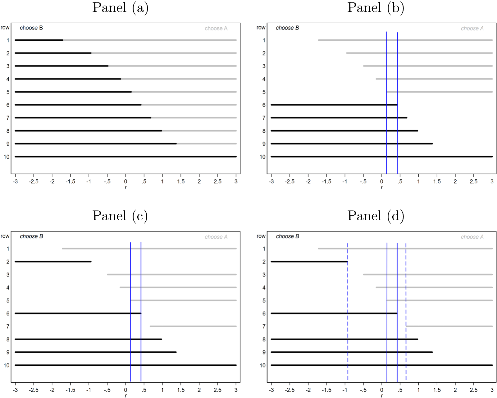


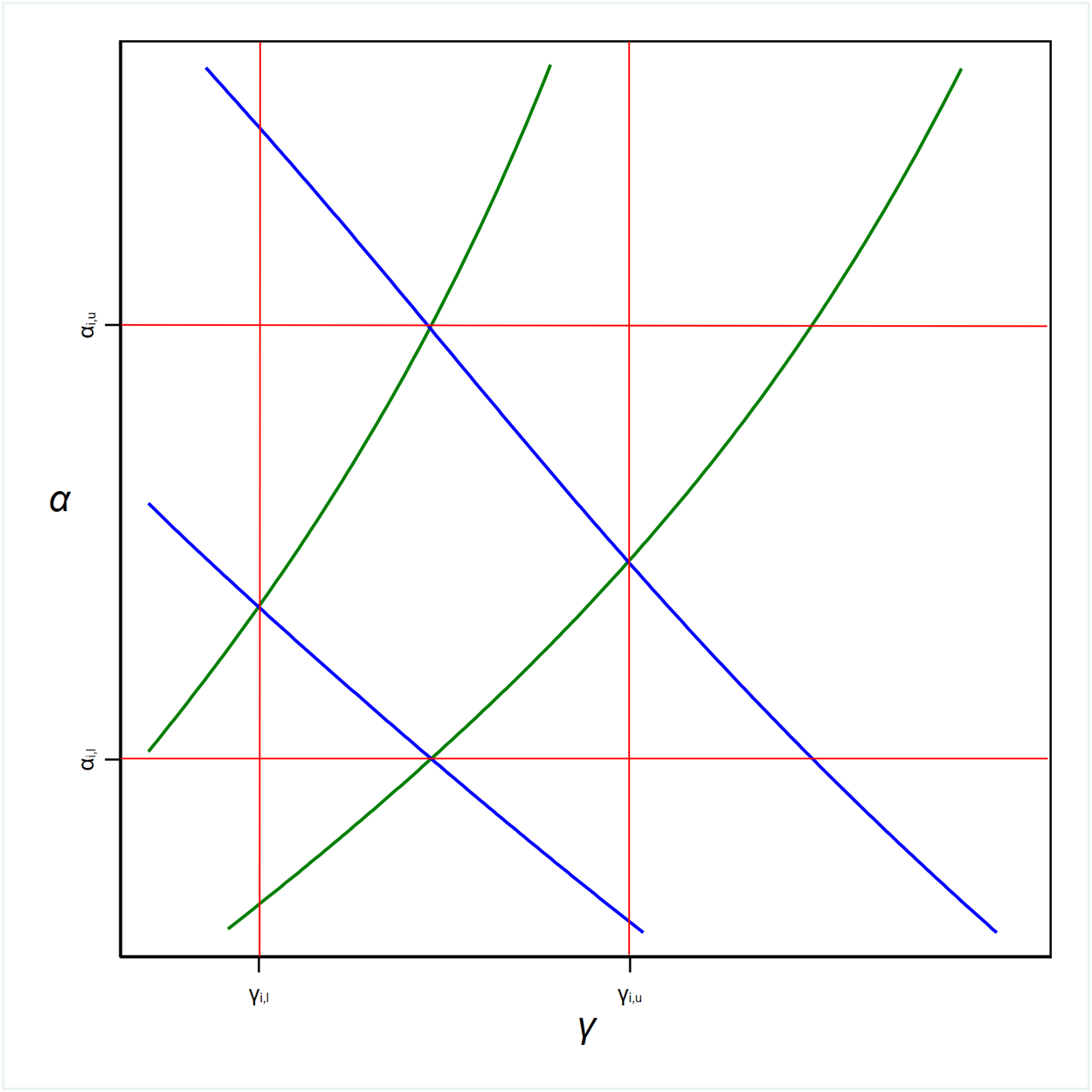


 Open access