

Introduction
Vostok Subglacial Lake in central East Antarctica represents an outstanding research target for a broad variety of disciplines (Reference Kapitsa, Ridley, Robin, Siegert and ZotikovKapitsa and others, 1996). For most investigations, a precise knowledge of the ice flow velocity field over the lake is a fundamental prerequisite. The ice flow velocity is an important input for the interpretation of the Vostok ice core, in particular for the determination of the depth–age relation and the inference of paleo-accumulation rates along the flowline through the drilling site (e.g. Reference PetitPetit and others, 1999; Reference VYa, Barkov and SalamatinLipenkov and others, 2000; Reference Parrenin, Rémy, Ritz, Siegert and JouzelParrenin and others, 2004; Reference Salamatin, Tsyganova, Popov, Lipenkov and HondohSalamatin and others, 2009). It also determines the transit time of an ice particle over the lake and is therefore crucial for the investigation of ice–water interactions (Reference Tsyganova and SalamatinTsyganova and Salamatin, 2004; Reference Filina, Blankenship, Thoma, Lukin, Masolov and SenFilina and others, 2008; Reference Salamatin, Tsyganova, Popov, Lipenkov and HondohSalamatin and others, 2009; Reference Thoma, Grosfeld, Mayer and PattynThoma and others, 2010) and the estimation of the water residence time (e.g. Reference Thoma, Grosfeld and MayerThoma and others, 2008). Knowledge of the ice flow velocity is also essential for the inference of surface accumulation rates from internal layers derived from radar-echo sounding (e.g. Reference Popov, VYa and EnalievaPopov and others, 2007) and for the prediction of the age of basal ice in the search of potential new drilling sites. The flow velocity field over the largest known subglacial lake allows unique insights into the glacial dynamics involved with the transition from grounded to floating and back to grounded ice (Reference PattynPattyn, 2003) and helps to constrain the location of a major ice divide. Finally, the flow velocity field is an important component of ice mass-balance estimates on this extended section of floating ice deep in the interior of the continent (Reference RichterRichter and others, 2008).
On the other hand, the Vostok Subglacial Lake region presents particularly difficult conditions for the determination of ice flow velocities. Remote-sensing techniques such as satellite interferometric synthetic aperture radar (InSAR) (Reference Goldstein, Engelhardt, Kamb and FrolichGoldstein and others, 1993) or feature tracking (e.g. Reference Scambos, Dutkiewicz, Wilson and BindschadlerScambos and others, 1992) are common tools for the inference of flow velocity fields. However, these techniques require ice surface features and/or identifiable reference points with known velocity (usually bedrock features) neither of which is present on the structureless ice surface over Vostok Subglacial Lake. In addition, short-term vertical movements of the surface of the ice floating on the lake due to tidal and atmospheric forcing (Reference WendtWendt and others, 2005) must be taken into account when extracting horizontal displacements from InSAR data. An attempt to infer ice flow velocities over Vostok Subglacial Lake from InSAR (Reference Kwok, Siegert and CarseyKwok and others, 2000) overestimated the flow velocity at Vostok station by ∼100% (Reference WendtWendt and others, 2006).
Reference Tikku, Bell, Studinger and ClarkeTikku and others (2004) interpreted internal ice layers mapped by airborne ice-penetrating radar over Vostok Subglacial Lake. Internal structures were tracked, which reflect the ice flow and are related to bedrock topographic features at the upstream lake shore. They can be interpreted as flowlines only under the condition that the ice flow pattern remains unchanged throughout the transit time between the upstream and downstream lake shore (Reference RossRoss and others, 2011). This approach is limited to the immediate lake area and is not able to provide estimates of the velocity magnitudes. Furthermore, this technique depends on the preservation and identification of the structures along their trajectory over the lake. Especially in the northern part of Vostok Subglacial Lake, flowline determination suffered from insufficiently preserved structures (Reference Tikku, Bell, Studinger and ClarkeTikku and others, 2004).
Ice dynamic modeling is another source of information that might constrain the regional flow velocity field. However, the Vostok Subglacial Lake region is also a challenge for ice flow modeling, for several reasons. First, the extremely small surface gradients over the lake, orientated perpendicular to the overall flow direction, are unfavorable for the application of simple modeling approaches such as balance velocities (e.g. Reference Cuffey and PatersonCuffey and Paterson, 2010). Second, bedrock relief, basal conditions and mean accumulation rate are only approximately known in the Ridge B–Vostok Subglacial Lake region. Third, the effects of accreted ice on both the temperature structure of the deeper part of the ice sheet and the basal friction on the downstream grounded area are not sufficiently well known. Fourth, this region is characterized by relatively low flow velocities and the presence of an ice divide, which makes the ice flow models extremely sensitive to small errors in the assumed boundary conditions. Finally, any model will be restricted by its ability to represent the physics of the real situation. Over recent years, a series of ice flow models for the Vostok Subglacial Lake region have been published and one of our objectives is to evaluate the extent to which the models of Reference Pattyn, De Smedt and SouchezPattyn and others (2004) and Reference Thoma, Grosfeld, Mayer and PattynThoma and others (2012) are able to represent ice flow velocities over the lake.
In situ observations of flow velocity, in this case derived from Global Navigation Satellite Systems (GNSS), are the best for evaluating the ice dynamics of the lake area. The difficulty in accessing this remote area, combined with the low temperatures, makes geodetic fieldwork a logistical challenge. Previous in situ observations of ice flow velocities (Reference Bell, Studinger, Tikku, Clarke, Gutner and MeertensBell and others, 2002; Reference WendtWendt and others, 2006; Reference RichterRichter and others, 2008) used the Russian Antarctic Vostok station as a logistic base and were therefore restricted to the southern part of the lake. Since 2006 we have participated in five convoys of the Russian Antarctic Expedition from Vostok station to Mirny and Progress stations and were thus able to extend our geodetic fieldwork to the central and northern parts of the lake.
For the first time, we present ice flow velocity vectors for 50 surface markers in the Vostok Subglacial Lake region, including the central and northern parts of the lake. We use our results to validate a recent ice flow model by Reference Thoma, Grosfeld, Mayer and PattynThoma and others (2012) and the flowlines derived by Reference Tikku, Bell, Studinger and ClarkeTikku and others (2004) from structure tracking in internal layers. Furthermore, we apply the flux-gate method (Reference Cuffey and PatersonCuffey and Paterson, 2010) to our results to estimate mean surface accumulation rates for the Ridge B–Vostok Subglacial Lake region.
Gnss Observations and Data Processing
Our geodetic fieldwork in the Vostok Subglacial Lake region commenced in the 2001/02 austral summer (Reference WendtWendt and others, 2006). The markers installed and observed during that season are limited to the Vostok station area and the southern part of the lake. In the following field season these markers were reoccupied and three additional markers were installed in the southern part of the lake. During the 2006/07 season, a joint Russian–German geophysical–geodetic traverse between Vostok and Mirny stations was carried out with logistic support from the Russian Antarctic Expedition. As a result, the geodetic fieldwork was extended to the central and northern parts of the lake and some of the previous markers in the vicinity of Vostok station were reoccupied (Reference RichterRichter and others, 2008). One year later the traverse was repeated. A number of additional GNSS markers were installed and observed in the central and northern parts of Vostok Subglacial Lake and several of the existing markers were reoccupied. In addition, a permanent GNSS station was installed at Vostok station. Between 2009 and 2011, in the course of two traverses between Vostok and Progress stations, the GNSS observations were repeated at most of the markers.
The distribution of the markers is shown in Figure 1. Additional details on the markers and their occupations are summarized in Table 1. All of these markers have been observed at least twice, with time-spans between 1 and 9 years. This allows an accurate determination of the marker velocities, since the accuracy generally increases with the time interval between first and last occupation (Reference WendtWendt and others, 2006).
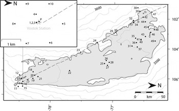
Fig. 1. Map of the Vostok Subglacial Lake region. The subglacial lake is shown in blue; the shoreline is derived from radio-echo sounding (Reference Popov and ChernoglazovPopov and Chernoglazov, 2011). Black dots denote the location of GNSS markers, numbered as in Table 1. Dashed line: convoy track Vostok–Mirny; contours: surface elevation according to Reference Bamber, Gomez-Dans and GriggsBamber and others (2009) at 20 m spacing. Inset shows the Vostok station area.
Table 1. Summary of the 50 GNSS markers and the determined ice flow velocity vectors in the Vostok Subglacial Lake region. For each marker (first column; numbers as in Fig. 1) the following details are given: the coordinates, the flow velocity magnitude v with its estimated uncertainty σv , the flow azimuth α with its estimated uncertainty σa , the flow velocity v M and azimuth α M according to the numerical ice flow model of Reference Thoma, Grosfeld, Mayer and PattynThoma and others (2012), the seasons of the first and last observation (01 denotes Antarctic field season 2001/02, 10 denotes season 2010/11, etc.), the number of occupations and the total amount of daily observation files. The flow velocities and flow directions refer to bedrock as the rotation of the Antarctic tectonic plate has been subtracted

The markers set up in the southern part of the lake during the first two seasons are 80 cm long wooden stakes, each with a screw on top onto which the GNSS antenna is mounted (Fig. 2; Reference WendtWendt and others, 2006). At their installation, the top of the markers was situated ∼30 cm above the snow surface. During the later seasons, however, due to snow accumulation the markers were found below the surface, and an extension rod of defined length was used to mount the antenna above the snow horizon. Each of these markers was complemented by two wooden reference stakes (10 m apart) arranged in a triangle. Before and after the GNSS occupations, the stability of the GNSS marker was verified by tape and leveling measurements within the triangle. The markers installed since 2006 are aluminum tubes 75–150 cm in length, with the top also ∼30 cm above the snow surface. We used an adapter tube to ensure an exact mounting of the GNSS antenna on top of the marker.

Fig. 2. Example of a GNSS marker in the southern part of Vostok Subglacial Lake (marker 9). The wooden stake extends to a depth of ∼60 cm into the firn. On top of the stake a special screw is fixed onto which the GNSS antenna is mounted. After the occupation, a plastic cap (grey) is used to protect the screw thread.
Geodetic GPS receivers (Trimble 4000SSi) and antennas (TRM33429.00) were used. From 2007, GLONASS (Global Navigation Satellite System) capable receivers (Trimble R7; Leica GRX1200+GNSS) and antennas (TRM57971.00; LEIAX1203+GNSS) were also employed. Dual frequency GPS (and GLONASS when tracked) code and phase observations were recorded. At each occupation we measured the antenna azimuth and the height of the antenna reference point with respect to the marker top and the local snow surface. Whenever possible, the same antenna was used during all occupations for a specific marker. The markers in the Vostok station area and in the southern part of the lake were usually occupied for 1–60 days per season (Reference WendtWendt and others, 2006; Reference RichterRichter and others, 2008). The observation of the markers in the central and northern parts of the lake had to comply with the tight convoy schedule. Here the occupations were typically of 6 hours, with a minimum of 2 hours.
The complete set of GNSS data from the Vostok Subglacial Lake region was homogeneously processed with the Bernese GPS software 5.1 (Reference Dach, Hugentobler, Fridez and MeindlDach and others, 2007). In addition to our campaign sites, 14 permanent tracking stations were included to integrate our data with the terrestrial reference frame IGS08 (Reference Rebischung, Griffiths, Ray, Schmid, Collilieux and GaraytRebischung and others, 2011), a GNSS-specific global station coordinate/velocity set aligned to the International Terrestrial Reference Frame ITRF2008 (Reference Altamimi, Collilieux and MétivierAltamimi and others, 2011). This set (see inset of Fig. 5 below), comprises 12 International GNSS Service (IGS) stations plus two receivers we operated at the Russian summer bases Leningradskaya and Russkaya. In our GNSS data analysis, we applied reprocessed products (GPS and GLONASS satellite positions, Earth rotation parameters). Up-to-date models were introduced to account for atmospheric signal delays and antenna phase center variations as well as tidal and loading effects (Reference Rülke, Dietrich, Fritsche, Rotacher and SteigenbergerRülke and others, 2008). Over the entire time interval spanned by our occupations all the pre-processed daily GNSS observation data files were used to derive daily normal equation systems. For the final parameter estimation, all daily normal equation systems were combined to obtain three-dimensional (3-D) site positions and velocities with respect to the IGS08 reference frame. Finally, the rotation of the Antarctic tectonic plate was subtracted from the horizontal velocity components. Therefore, the resulting horizontal velocity vectors refer to bedrock (Reference WendtWendt and others, 2006; Reference RichterRichter and others, 2008).
For a realistic assessment of the positioning accuracy we made use of the continuous GNSS data of the permanent tracking station at Vostok and the IGS stations. Daily normal equation systems were solved separately to obtain site positions for each individual day. Station position time series were then generated by computing the differences between the daily coordinate solutions and the combined linear model. Afterwards, a combined noise model (white and flicker noise) was applied to the residual position time series. For ten permanent stations, the mean root-mean-square (rms) values are 2.4 mm (north component) and 1.8 mm (east component). We adopt an rms of 2.4 mm for both horizontal coordinate components valid for a 24 hour observation interval. However, in the northern part of Vostok Subglacial Lake, several markers were observed for <24 hours. We assessed the effect of shorter occupation times on the positioning accuracy by comparing coordinate estimates derived from 1 and 2 hour observation intervals with the corresponding 24 hour mean. Figure 3 shows the results for marker 1 at Vostok station on 6 January 2008. Here the scatter of the 2 hour estimates reveals rms values of 2.0 mm (north) and 2.8 mm (east). The occupations in the Vostok Subglacial Lake area lasted for >2 hours (usually 6 hours) in all cases. Therefore, we allow for an additional uncertainty of 2.8 mm for both horizontal components for all occupations <24 hours, which results in a GNSS positioning accuracy of 5.2 mm.

Fig. 3. Assessment of the accuracy of GNSS positioning at Vostok station (marker 1) for observation intervals of <24 hours. The complete 24 hour observation file from 6 January 2008 was split into 24 intervals of 1 hour (grey triangles) and 12 intervals of 2 hours (black dots). For each of these individual intervals (a) the north (ΔN) and (b) the east (ΔE) coordinate components were determined and their deviation from the complete daily solution is shown. The corresponding rms values are included.
In addition we consider uncertainties in the exact horizontal relocation of the antenna phase center with respect to an ice fixed point. This uncertainty affects the entire occupation uniformly and is composed of potential contributions from residual antenna phase eccentricities, from the installation of the antenna onto the marker and from slight instabilities of the marker. The IGS antenna phase center variation models were applied in the data processing, and, whenever possible, the same antenna was used for all occupations of a specific marker. The relocation of the antenna on the marker was achieved by forced centering (Fig. 2) for the southern markers and by a tightly fitting adapter tube for the northern markers. Marker stability was checked before and after each occupation, and that of the southern markers was also checked with respect to the reference stakes. Thus, in addition to the daily GNSS positioning uncertainty, we apply to each occupation and both horizontal components an additional uncertainty of 4 mm for the wooden markers in the southern part of the lake and of 10 mm for the aluminum markers.
The resulting total positioning uncertainty, obtained by the sum of the GNSS positioning uncertainty and the occupation uncertainty for the first and last observation days, propagates to the ice flow azimuths and velocities as a function of the time-span covered by the repeated observations. We therefore obtain individual accuracy estimates for each marker, which are included in Table 1. In general, the velocity and azimuth uncertainties are <20 mm a−1 and 1°, respectively. These uncertainty estimates are considered to be very conservative.
For our first markers in the southern part of the lake, the horizontal velocity vectors presented here and resulting from observation data from the period 2001–11 agree very well with those published by Reference WendtWendt and others (2006) based on observations spanning just 1 year. This confirms, first, the robustness of our accuracy estimates and, second, that the assumption of a linear movement over the observation interval is appropriate. This is also illustrated in Figure 4. In Figure 4a, the horizontal displacement of marker 1 at Vostok station, as observed during five occupations between 2002 and 2010, reveals a very good fit of the daily coordinate solutions (black dots) with the derived linear velocity (red line). In Figure 4b, the deviations of the north (blue) and east (green) components of the daily coordinate solutions from the detrended linear velocities (horizontal grey lines) are shown over time. Also included are the mean residual coordinate components for each occupation (black dots) with the adopted uncertainty estimates, comprising the contributions of the GNSS positioning and antenna phase centering. This confirms that the adopted uncertainty measures are rather conservative with regard to the scatter of the daily solutions about the occupation mean and the fit to the linear velocity. The accuracy estimates are backed up further by the agreement of the velocities derived for the permanent station and markers 1–3, which are separated by <100 m.

Fig. 4. Time series of daily coordinate solutions at Vostok station (marker 1). (a) Topocentric horizontal coordinate change of 133 daily solutions (black dots) between 2002 and 2010. Red line: linear velocity derived from the observations. (b) Residual north (blue) and east (green) coordinate components after subtraction of the derived velocity (horizontal lines: vertically offset by ±10 mm for legibility; dashed lines: estimated velocity uncertainty) over time. For each of the five occupations (campaigns) the mean residual coordinates (black dots) and the adopted uncertainty estimates (bars) are included.
Results
For each of the markers the azimuth and velocity of the ice flow with respect to bedrock were obtained from the GNSS data processing. They are given in Table 1 and depicted as vectors in Figure 5. For the markers within the lake area, the observed ice flow velocity components are representative for the entire vertical ice column because there is no basal friction affecting the flow (Reference Tikku, Bell, Studinger and ClarkeTikku and others, 2004).

Fig. 5. Ice flow velocity vectors determined by repeated GNSS observations in the Vostok Subglacial Lake region. Black dots: location of GNSS markers; red vectors: ice flow velocity vector (see scale at the right); grey vectors: ice flow velocity vectors for the marker locations as predicted by the ice flow model of Reference Thoma, Grosfeld, Mayer and PattynThoma and others (2012); orange lines: structures tracked by Reference Tikku, Bell, Studinger and ClarkeTikku and others (2004) in englacial layers; thick grey line: shoreline of Vostok Subglacial Lake. Inset shows location of the region under investigation (red spot) in central East Antarctica. Included are the locations of the 14 permanent GNSS stations used in the GNSS data processing for the realization of the terrestrial reference frame.
According to the ice flow vectors shown in Figure 5, the general flow direction over the lake is from west to east. The ice flow directions in the southern and northern part diverge, with a strong south component in the southern part and a deviation towards north in the northern part of the lake. The maximum velocities are observed in the southernmost part of the lake, peaking at 2.09 m a−1 at marker 11. In the northern part of the lake the velocities keep slightly below 2 m a−1. In the central part (markers 22–30) they are considerably smaller, ∼1 m a−1.
Figure 6 illustrates the relative change in the flow velocity along five profiles orientated approximately parallel to the flow direction. The markers of each profile are located close to, but not exactly on, the same flowline. The locations of the profiles are included in Figure 7.

Fig. 6. (a) Relative change of the ice flow velocity along five profiles a–e approximating flowlines. Over the distance along-flow from the upstream (western) shore the relative change of the observed velocity magnitude Δv from marker to marker is shown (black dots: numbers according to Fig. 1; dot diameter corresponds approximately to a velocity uncertainty of 10 mm aȡ1); the arrow indicates the flow direction. The profiles are offset by an arbitrary constant velocity for better legibility. Grey shaded areas denote parts of the flowlines where the ice is grounded. (b) Profiles of the ice thickness (red; orange band indicates the uncertainty of a single value of ±42 m) and the surface elevation above the TOPEX ellipsoid (green; Reference Ewert, Popov, Richter, Schwabe, Scheinert and DietrichEwert and others, 2012; uncertainty ±1 m) along profile b. The location of profiles a–e is shown in Figure 7.

Fig. 7. Map of the Vostok Subglacial Lake–Ridge B region. Vostok Subglacial Lake is shown in blue. Colored areas show the four surface segments A–D for which mean surface accumulation rates were estimated from ice flow velocities and ice thickness. Large black dots indicate the GNSS markers used as flux gates. Included in each segment are the obtained mean surface accumulation rates (mmw.e. a−1) with their formal uncertainties. Red square: location of the snow pit where the accumulation was determined by β-radioactivity; tiny black triangles: location of 65 stakes at which surface accumulation was measured (western profile section); tiny white triangles: location of ten accumulation stakes (eastern profile section); dots: GNSS markers; dashed line: convoy track Vostok–Mirny; contours: surface elevation according to Reference Bamber, Gomez-Dans and GriggsBamber and others (2009) at 20 m spacing. Thin lines connecting GNSS markers depict the flowline profiles a–e shown in Figure 6.
In the northern part of the lake (Fig. 6; profiles a and b), passing the western upstream grounding line, the ice flow slows down. It seems to recover 20 (profile b) to 40 km (profile a) downstream of the western grounding line. About halfway across the lake (Fig. 6; profile a: markers 46–49; profile b: 35–37; profile c) the flow velocity begins to increase slightly. The southern profiles (Fig. 6; profiles d and e) reveal a strong acceleration as the ice approaches the eastern (downstream) grounding line. This acceleration seems to continue beyond the eastern grounding line (Fig. 6; profile e).
Discussion
These observed flow velocity variations contradict the general concept that over a subglacial lake the ice velocity rises to a local maximum (e.g. Reference Cuffey and PatersonCuffey and Paterson, 2010). They are also opposed to the results of an attempt to model the impact of a subglacial lake on the flow velocity field (Reference PattynPattyn, 2003). The surface elevation and ice thickness along profile b is included in Figure 6b. The surface elevation drops quickly from 3549 m (by 10 km upstream of the groundling line) to 3516 m (1 km downstream) and rises quickly again to 3528 m (17 km downstream). This minimum marks the topographic depression revealed previously by Reference Rémy, Shaeffer and LegrésyRémy and others (1999). From their first-order analysis, Reference Rémy, Shaeffer and LegrésyRémy and others (1999) concluded that the ice flow in the transition zone between strong and weak basal friction is characterized by extension. However, this is not supported by the slowdown observed along profile b.
Our results along profile e, i.e. along the flowline through Vostok station, allow us to revise the transit time estimates by Reference WendtWendt and others (2006). We include data from a new marker (marker 18) 26 km upstream of Vostok station, and additional observations for the remaining sites of the profile. Moreover, the location of the grounding line at the eastern and western shores as well as around the bedrock island close to the western shore has been improved based on radio-echo data (Reference Popov and ChernoglazovPopov and Chernoglazov, 2011). According to the results presented here, the travel time of an ice particle from the western to the eastern shoreline (a distance of 62.5 km) amounts to 38.5 ka. As in Reference WendtWendt and others (2006) we have assumed a constant acceleration of the flow velocity from the western shore through Vostok station, which implies a velocity increase from 1.25 m a−1 at the western shore to 2.03 m a−1 at the eastern shore. The transit time from the eastern shore of the bedrock island located near the western shore, down to the eastern lake shoreline (48.3 km) amounts to 27.9 ka. For the transit time from the bedrock island to Vostok station (42.8 km), i.e. the drilling site of the Vostok ice core, we obtain 25.2 ka. These transit time estimates confirm the results of Reference WendtWendt and others (2006). They agree with the previously published results within 3%. These transit time estimates are based on present-day flow velocities. Taking into account variations in flow velocity over time, Reference Salamatin, Tsyganova, Popov, Lipenkov and HondohSalamatin and others (2009) obtained a transit time of 40 ka between the western shore and Vostok station. For the accumulation anomaly deposited 26 ka ago at the western lake shore and detected by Reference Leonard, Bell, Studinger and TremblayLeonard and others (2004) in radio-echo data, we now obtain a travel time of 24.95 ka, i.e. within 5% of the expected age. This confirms the conclusion of Reference WendtWendt and others (2006) that the flow regime along this flowline has not changed significantly over the past 20 ka. Our new velocity profile yields a transit time of 14.2 ka from marker 18 to 1. For this transect, 60 m of accreted basal ice was detected by Reference Bell, Studinger, Tikku, Clarke, Gutner and MeertensBell and others (2002) from radio-echo data. This leads to a mean accretion rate of 4.2 mm a−1, again in agreement with Reference WendtWendt and others (2006).
Our results show that Reference Kwok, Siegert and CarseyKwok and others (2000) overestimated the flow velocities in the central and southern part of the lake by a factor of 2 and that their flow directions in the southern half of the lake point too far northwards by up to 30°.
Comparison with Ice Flow Models
Numerical ice flow modeling
Reference Thoma, Grosfeld, Mayer and PattynThoma and others (2012) coupled a full-Stokes 3-D ice flow model with a 3-D lake flow model to simulate the ice flow velocity field in the Vostok Subglacial Lake region and to investigate its sensitivity to different boundary conditions. The flow velocities and azimuths resulting from this model at the locations of our GNSS markers are included in Table 1 and Figure 5. The modeled velocities vM and azimuths αM were obtained by a digitization and inverse projection of the velocity contours and flow directions in figure 3a of Reference Thoma, Grosfeld, Mayer and PattynThoma and others (2012) and a subsequent interpolation onto the marker locations. In the southern part of the lake, the modeled ice flow directions agree fairly well with the observed directions. However, the slight eastward deflection of the observed vectors at the southeasternmost markers (11, 12, 15) is not reflected in the model. In the central and northern parts of the lake (markers 23–49) the observed and modeled flow directions disagree by 18° on average, with the observed vectors pointing farther northwards. All the ice flow velocities are clearly overestimated by the model by a factor of 2.5 on average. The largest factors, reaching 3.5, are observed in the central part of the lake (markers 22–28). The disagreement of both azimuths and velocities becomes equally clear at the markers at the upstream (western) lake shore. Thus the ice flow is already not correctly predicted where the ice enters the lake, but also the relative velocity changes within the lake do not agree with the observations. For example, along profile a (Fig. 6), the model predicts an acceleration from west to east up to marker 45, and from there the modeled velocities decrease. In contrast, the observed velocities along this profile show a slowdown up to marker 46, followed by a slight acceleration. For Vostok station the model yields a velocity of 4 m a−1, which is double the observed flow velocity.
In a prior attempt to model the ice flow field across the lake, Reference Pattyn, De Smedt and SouchezPattyn and others (2004) used a thermomechanical higher-order ice-sheet model. Their ‘lake experiment’ (LE) model yielded flowlines that are inconsistent with our observed flow directions. At all marker sites the modeled flowlines are orientated too far north; except for the markers situated at the western shore, the azimuth differences exceed 45°. The modeled flow velocities increase from south to north, exceeding 10 m a−1 in the northern part of the lake, which is also not consistent with our observed velocities. In the ‘lake with buoyancy experiment’ (LBE) flowlines were obtained for the southern part of the lake that are comparable with the observed azimuths. In the northern part of the lake (markers 29–49), however, the disagreement of the modeled flowlines with the observed flow directions is even worse than for the LE experiment. Also, the flow velocities resulting from the LBE experiment do not fit the observations (5 m a−1 at Vostok station, >20 m a−1 in the northern part).
Results from structure tracking
Reference Tikku, Bell, Studinger and ClarkeTikku and others (2004) tracked structures in englacial layers identified in ice-penetrating radar data over Vostok Sub-glacial Lake. The structures originate at bedrock topographic features at the upstream (western) lake shore and result from the motion of the ice sheet over these features. Generally, they reflect the cumulative evolution of the ice flow pattern since their formation (Reference RossRoss and others, 2011). In cases where the flow regime did not change throughout the transit time of the ice from the upper to the lower lake shore, these structures represent flowlines. If the flow pattern changed gradually (with a constant rate), the structures would still be close to present-day flowlines near the upper shore (where the structures are youngest), but would diverge progressively from recent flow directions downstream (as the age of the structures increases). A short-term event that altered the flow pattern only momentarily in the past will manifest itself in a bend of the structures, i.e. in a constant azimuth offset of the structure orientation with respect to the present local flow directions from a point of the structure. The time when such an event occurred could then be constrained based on the distance of that point along the flowline to the upper shore and the present-day flow velocity (Reference RossRoss and others, 2011).
The structures tracked by Reference Tikku, Bell, Studinger and ClarkeTikku and others (2004) across Vostok Subglacial Lake are included in Figure 5. In general, good agreement is found between the structure orientation and the flow directions observed at our markers. In the northern part of the lake (markers 30–49), GNSS shows a stronger north component of the ice flow than the results of the structure tracking. At markers 35, 36, 37 and 40 the azimuths differ by ∼10°. Also for the northernmost structures this difference is of the same sign and similar magnitude. In the central part of the lake (markers 22, 25–28), there also appear to be small deviations of the structures from the observed flow azimuths, with a tendency of the GNSS vectors further towards the north. Here, however, these differences seem to be caused to a large extent by the limited spatial resolution of the structure-tracking results (e.g. markers 22 and 26). In the southern part of the lake (markers 1–21), excellent agreement is found between the structures and the observed flow directions. This proves that (1) the ice flow regime over the southern part of the lake has not changed significantly since the time when the structures were formed at the western lake shore and (2) over the lake the deep ice flows identical to the ice surface.
The systematic 10° azimuth offset found in the northern part of the lake might be interpreted as an indication for a change in the ice flow direction since the formation of the structures. However, the spatial distribution of the azimuth offsets does not suggest a straightforward plausible reconstruction of flow direction changes. For example, at marker 44 the azimuth difference is smaller than at marker 42 although it is farther from the western shore. A rather large difference is also found at marker 30 directly at the western shore, but this might result from local effects related to the transition at the grounding line and steeper surface gradients. This illustrates, however, the limitation in the spatial resolution of both the structures and the GNSS markers. Moreover, in the northern part of the lake the structures are not well preserved (Reference Tikku, Bell, Studinger and ClarkeTikku and others, 2004). Here the structures could not be tracked in the gridded internal-layer elevation maps, but only in the flight lines parallel to the lake axis with a spacing of 11.25 or 22.5 km. A horizontal positioning uncertainty of 2 km (Reference Tikku, Bell, Studinger and ClarkeTikku and others, 2004) at a spacing of 11.25 km corresponds to an azimuth error of 10°. In addition, the inferior preservation of the structures could have introduced additional uncertainties in the structure identification and localization in the northern part of the lake. Therefore, we may also interpret the azimuth differences in the northern part of the lake as an effect of limited resolution and accuracy in the structure-tracking results rather than as a change in the ice flow regime.
Application: Accumulation Rate Estimates for Ridge B Region
The ice flow vectors obtained for a selection of the markers are used to constrain the surface accumulation rates upstream of Vostok Subglacial Lake towards Ridge B. The flow velocity vectors are complemented by ice thickness profiles between the GNSS markers obtained from radio-echo sounding (Reference Popov, Masolov and LukinPopov and others, 2011; Reference Siegert, Kennicutt and BindschadlerSiegert and others, 2011). We use pairs of markers as flux gates and determine the annual ice mass passing through each pair. It has been shown that the ice sheet around Vostok station is close to steady state (Reference RichterRichter and others, 2008). Under this condition, the mass flux through the gate equals the mean net surface accumulation rate within the surface segment bounded by the upstream flowlines through marker pairs. According to estimates of the relaxation time of the East Antarctic ice sheet (e.g. Reference Van der VeenVan der Veen, 1999), a change in surface accumulation will manifest itself in the flux through the gate with a delay in the order of 10 ka. The advantage of applying this approach to Vostok Subglacial Lake is that the ice floating on the lake’s water experiences no basal friction and the observed surface velocities can be regarded as representative for the entire vertical ice profile. On the other hand, further to the east within the lake, the poorly constrained effects of basal melting and accretion increase. We therefore chose five markers (23, 24, 30, 32, 47) close to the grounding line of the western lake shore, forming four approximately equidistant flux gates normal to the general ice flow direction (Fig. 7).
The annual ice volume flux through the gates is easily obtained from the flow velocity vectors, the distance between both markers, and the mean ice thickness along the profile between both markers. The ice flow vector is assumed to change linearly with the distance between the two bounding markers. The volume is converted into mass by applying the mean density along the vertical profile. The density profile is assumed to be identical to that retrieved from the Vostok ice core (Reference Lipenkov, Salamatin and DuvalLipenkov and others, 1997) for the upper 2000 m and of constant density (923 kg m−3) below 2000 m depth (Reference RichterRichter and others, 2008).
The ice surface digital elevation model (DEM) derived by Reference Bamber, Gomez-Dans and GriggsBamber and others (2009) from the combination of laser and radar altimetry data was used to retrieve the flowlines from the GNSS markers upstream. The DEM was smoothed by applying a 100 km Gaussian filter (Reference Parrenin, Rémy, Ritz, Siegert and JouzelParrenin and others, 2004). The flowline was then determined following the maximum surface gradient up to a point on Ridge B where the flowlines converge. For each flux gate the surface area of the segment bounded by the corresponding pair of flowlines was calculated. In order to assess the impact of the flowline determination on the calculated surface areas, this step was repeated, applying three different Gaussian filter widths for the DEM smoothing and alternatively using an Ice, Cloud and land Elevation Satellite (ICESat) DEM (Reference Ewert, Popov, Richter, Schwabe, Scheinert and DietrichEwert and others, 2012). Applying a filter width of 50 km changes the calculated surface area of segment C at most by almost 5%; for segments A, B and D the changes amount to 0.1%, 0.7% and 1.6%, respectively. Using the alternative DEM changes the surface areas by <0.5% in all cases. The flowline azimuths at the GNSS markers were compared with the ice flow directions observed by GNSS. Among the combinations of the two DEMs with four different filter widths, the best agreement is found for the model of Reference Bamber, Gomez-Dans and GriggsBamber and others (2009) with 100 km Gaussian filtering. For nine markers, the mean azimuth difference amounts to 0.16°, with a standard deviation of 5.85°. Therefore, we use this combination of DEM and filter in further computations.
The mean surface accumulation rate for each surface segment is obtained by dividing the annual ice mass flux through the gate by the surface area of the segment. The results with their formal errors are included in Figure 7. For the four segments, the following mean surface accumulation rates (mm w.e.a−1) are obtained: 23.4 ± 0.3 (segment A), 26.1 ± 0.3 (segment B), 28.5 ± 1.4 (segment C) and 34.4 ± 0.6 (segment D). The stated formal errors are obtained by propagating the uncertainties of the flow velocities (10 mm a−1;cf. Table 1), the marker positioning/gate width (![]() ), the ice thickness (42 m), the mean density (1 kg m−3) and the individual uncertainty of the surface area of each segment. The formal errors are probably too optimistic. The impact of uncertainties in the flowline determination, as well as deviations from the assumptions of linear changes of ice flow vectors and identical flow at the ice surface as at the base, are difficult to quantify. Even if no sliding occurred at the ice base beneath the flux gates, our surface velocities would overestimate the vertically integrated velocities by no more than 20% (Reference Cuffey and PatersonCuffey and Paterson, 2010). However, a substantial contribution of basal sliding is expected within a 10 km wide transition zone along the lake shore (Reference Rémy, Shaeffer and LegrésyRémy and others, 1999). Altogether, a relative error of the derived mean accumulation rates of 10% is a reasonable estimate.
), the ice thickness (42 m), the mean density (1 kg m−3) and the individual uncertainty of the surface area of each segment. The formal errors are probably too optimistic. The impact of uncertainties in the flowline determination, as well as deviations from the assumptions of linear changes of ice flow vectors and identical flow at the ice surface as at the base, are difficult to quantify. Even if no sliding occurred at the ice base beneath the flux gates, our surface velocities would overestimate the vertically integrated velocities by no more than 20% (Reference Cuffey and PatersonCuffey and Paterson, 2010). However, a substantial contribution of basal sliding is expected within a 10 km wide transition zone along the lake shore (Reference Rémy, Shaeffer and LegrésyRémy and others, 1999). Altogether, a relative error of the derived mean accumulation rates of 10% is a reasonable estimate.
The obtained accumulation rates appear to be consistent among themselves as well as when compared with the few available accumulation data in the region under investigation. They show a steady increase in the mean accumulation rate from south to north. The β-radioactivity analysis in a snow pit located close to flux gate D (Fig. 7) yields a mean accumulation rate of 35 mm w.e. a−1 over 30 years (Reference Lipenkov, Yekaykin, Barkov and PursheLipenkov and others, 1998). This is in excellent agreement with our result for segment D. At Vostok station a long-term (1816–2004) mean accumulation rate of 20.6 ± 0.3 mm w.e.a−1 was derived from borehole studies and deep pits (Reference Ekaykin, Lipenkov, Kuzmina, Petit, Masson-Delmotte and JohnsenEkaykin and others, 2004). This confirms the regional trend of increasing surface accumulation from south to north. In fact, both the glaciological results and our geodetic approach yield a comparable north–south accumulation gradient: 0.06 mm a−1 km−1 between the snow pit and Vostok station compared with 0.10 mm a−1 km−1 between our segments A and D.
Accumulation measurements were carried out at accumulation stakes set up in early 2008 at 2 km intervals along a 188 km long approximate ice flowline from the northwestern shore of Vostok Subglacial Lake up to Dome B (Fig. 7). The easternmost ten stakes (profile km 0 to km 18) were remeasured in early 2010, yielding a mean accumulation rate for this profile section of 37 mm w.e. a−1 (accounting for the density of the upper 20cm snow layer measured at each stake and the snow settling correction). The remeasurement of stakes 28–94 (profile km 56 to km 188) in early 2012 revealed a mean accumulation rate of 29 mm w.e.a−1 over 4 years. The stake profile follows roughly the flowline dividing the surface segments C and D. Its eastern (lower) section indicates an accumulation rate slightly exceeding the flux through gate D, whereas the western section yields an accumulation slightly above but very close to the flux through gate C. In the flux gate analysis, the longitudinal changes in the accumulation rate are integrated. Roughly speaking, the accumulation rates in the upper parts of the surface segments have a smaller impact on the observed flux than rates in the lower part, because they are represented by a smaller fraction of the surface area due to the generally divergent ice flow down from the ice divide. Thus the flux corresponding to the accumulation rates observed along the stake profile amounts to a value between those obtained for flux gates C and D. We conclude, therefore, that the flux gate results are consistent with the stake measurements. This consistency supports the assumption of steady state in the region under investigation.
The mean accumulation rates obtained for the surface segments west of the northern part of the lake and their increase from south to north complement very well the accumulation map derived by Reference Popov, Kharitonov and ChernoglazovPopov and others (2004) from snow pits in the southern part of Vostok Subglacial Lake. The accumulation map derived by Reference Arthern, Winebrenner and VaughanArthern and others (2006) from field measurements and remote-sensing data overestimates the accumulation rates in the Vostok Subglacial Lake–Ridge B region by ∼10 mm w.e.a−1, i.e. by 25–50%. It predicts the north–south gradient revealed by the flux-gate method over the four surface segments, but the differences (model minus flux-gate) increase from 9 (segment D) to 18 mm w.e.a−1 (segment A). Differences of similar magnitude are also found with respect to the in situ results at the snow pit close to flux gate D (7 mm w.e. a−1) and Vostok station (16 mm w.e. a−1). The error estimates provided along with the map thus seem to be too small by a factor of 2–5 in this region.
Conclusions
The velocity magnitudes and azimuths of the ice flow at 50 surface markers in the Vostok Subglacial Lake region have been determined from repeated GNSS observations with typical accuracies of 1 cm a−1 and 0.5°, respectively. These provide the first reliable information on the ice flow dynamics in the northern part of the lake.
The flow velocities, especially in the northern part of Vostok Subglacial Lake, are smaller than previously assumed. Within the lake area they do not exceed 2 m a−1. The flow direction diverges southeastwards in the southern part and east- northeastwards in the northern part of the subglacial lake.
Relative velocity changes observed along flowlines across the grounding lines reveal the impact of the lake and its shore. In the northern part of the lake a steady slowdown is observed from upstream of the western shore towards the central lake axis, followed by slight acceleration. Thus the lake seems to coincide here with a regional flow velocity minimum. In the southern part of the lake, acceleration is observed that continues beyond the downstream grounding line.
This is not reflected by existing numerical ice flow models (Reference Pattyn, De Smedt and SouchezPattyn and others, 2004; Reference Thoma, Grosfeld, Mayer and PattynThoma and others, 2012), suggesting that the physical processes involved in the flow of ice over the extended water surface of Vostok Subglacial Lake are not yet fully understood. To date, these numerical models are not able to realistically represent the flow velocity field over the lake. This emphasizes the importance of in situ observations. Our results (Table 1) provide a reliable basis for the improvement of numerical ice flow models in the Vostok Subglacial Lake region.
Based on the observed ice flow vectors, complemented by ice thickness data, mean surface accumulation rates were estimated for four surface segments between Ridge B and Vostok Subglacial Lake. The accumulation rates, varying between 23 and 34 mm w.e.a−1, show a clear increasing trend towards the north and are consistent with glaciological results.
Acknowledgements
We thank the staff at Vostok station and the participants in the convoys during the 47th, 48th, 52nd, 53rd, 55th, 56th and 57th Russian Antarctic Expeditions for their valuable support of the fieldwork. This work was funded by the German Research Foundation DFG (grants DI 473/20, DI 473/34, DI 473/38) and the Russian Foundation of Basic Research (grant 10-05-91330-NNIO-a). We thank two anonymous reviewers and the editor T. Scambos for valuable comments.


