


1 Introduction
In this article, we propose a regularized multilevel multinomial regression (RMMR) model for select-all-that-apply (SATA) response variables with high-dimensional predictors. The proposed RMMR model is motivated by the dataset published in Helwig et al. (Reference Helwig, Sohre, Ruprecht, Guy and Lyford-Pike2017). In their study,
$n = 802$
 participants were asked to rate their perceptions of 27 computer-animated facial expressions, which systematically varied according to three dimensions (angle, extent, and dental show). Participants were given a list of seven emotions (happy, sad, anger, contempt, fear, surprise, and disgust) and asked to select one or more emotions that best described the facial expression. Note that each participant could select 0 (not present) or 1 (present) for each of the seven emotions, which resulted in SATA data. Each participant rated anywhere from 1 to 8 facial expressions (mode of 3), and about 72% of the participants rated between 2 and 4 expressions. Thus, the binary emotion ratings data of Helwig et al. (Reference Helwig, Sohre, Ruprecht, Guy and Lyford-Pike2017) can be treated as SATA data with a multilevel structure, and the goal is to connect the SATA response probabilities to the properties of the facial expressions.
The 27 computer-animated facial expressions were designed by taking all combinations (low, medium, and high) of the three dimensions (angle, extent, and dental show), see Figure 1. In the analyses conducted by Helwig et al. (Reference Helwig, Sohre, Ruprecht, Guy and Lyford-Pike2017), the three smile design dimensions were encoded as ordinal factors, such that each of the 27 facial expressions was described by a three-dimensional ordinal vector. These authors then used a mixed-effects smoothing spline ANOVA model (Gu, Reference Gu2013; Gu & Ma, Reference Gu and Ma2005b), also known as a generalized additive mixed model (Wood & Scheipl, Reference Wood and Scheipl2020; Wood, Reference Wood2017), to connect the facial expression properties to participants’ ratings. A benefit of their approach was its potential to produce parsimonious interpretations; however, Helwig et al. (Reference Helwig, Sohre, Ruprecht, Guy and Lyford-Pike2017) ultimately found that a three-way interaction model was preferred, which complicated the interpretation. A limitation of their approach is that each dimension was quantified using ordinal information (low, medium, and high), which provides a rather rudimentary measure of each facial expression’s spatial properties.
Reproduction of Figure 1 from Helwig et al. (Reference Helwig, Sohre, Ruprecht, Guy and Lyford-Pike2017).

Figure 1 Long description
A matrix of 27 facial renders of a bald male character against a blue and gray background. The panels are organized into three large blocks from left to right based on Mouth Angle: low, medium, and high. Within each block, the vertical Y axis represents Dental Show (low, medium, high from bottom to top) and the horizontal X axis represents Smile Extent (low, medium, high from left to right).
* Mouth Angle low block (left): Panels 1 through 9. The bottom row (low Dental Show) shows closed lips. The top row (high Dental Show) shows visible upper teeth. As Smile Extent increases from left to right, the width of the mouth increases.
* Mouth Angle medium block (center): Panels 10 through 18. The corners of the mouth are pulled further upward compared to the first block. Panel 18 (top-right of this block) shows a wide smile with significant tooth exposure.
* Mouth Angle high block (right): Panels 19 through 27. The mouth corners are at their highest elevation. In the top row (high Dental Show), the smile is most pronounced, with panel 27 showing the maximum Smile Extent, Dental Show, and Mouth Angle.
Each panel is numbered in the top-left corner from 1 to 27. The faces maintain consistent eye and brow expressions while only the mouth region varies according to the three parameters.
Using ordinal information (instead of continuous information) to quantify the 27 smiles has important consequences for the generalizability of the modeling results. Specifically, when using the ordinal quantification, the model predictions can only be formed at the 27 faces used in the study, which prohibits generalization of the results to smile shapes that are similar to (but not exactly equal to) one of the 27 faces used in the original study design. Note that if it were possible to encode each facial expression’s shape using continuous information, then this would greatly improve the generalizability of the modeling results. In particular, using continuous measures to quantify each of the 27 smiles would make it possible to predict/interpret the emotions perceived from faces that are within the spatial range of—but not exactly equal to one of—the 27 faces used in the study.
In this article, we propose an approach for quantifying the shape of each smile and connecting these shape properties to the perceived emotions. Borrowing techniques from statistical shape analysis (Bharath & Kurtek, Reference Bharath and Kurtek2020; Dryden & Mardia, Reference Dryden and Mardia2016; Webster & Sheets, Reference Webster and Sheets2010), we propose to place landmarks at key locations on each smile (see, e.g., Ghimire & Lee, Reference Ghimire and Lee2013; Iyer et al., Reference Iyer, Rahul, Nersisson, Zhuang, Joseph Raj and Refayee2021), and then register the landmarks in a common spatial coordinate system. We then propose using an RMMR model to connect the spatial coordinates to the emotions perceived from each of the 27 faces. We also propose a dimension reduction approach for more efficient and interpretable handling of the landmark-based inputs to the RMMR model. Finally, we demonstrate how the proposed landmark-based approach can be used to predict emotional perceptions of smiles that are similar to (but not identical to) the 27 smiles used in the study’s design, which allows for more nuanced understandings of how subtle changes in a smile’s shape relate to its perception.
2 Literature background
2.1 Representing facial features
Over the past half century, the systematic representation of facial features has drawn a considerable amount of research interest in the fields of psychology, sociology, biology, medicine, and computer science (Ekman, Reference Ekman1957; Ekman & Friesen, Reference Ekman and Friesen1971). One of the most influential systems is Ekman and Friesen’s Facial Action Coding System (FACS), which offers an anatomically based method for decomposing any facial expression into specific, visually distinct movements called action units (AUs) (Ekman & Friesen, Reference Ekman and Friesen1978). In the FACS, the AUs correspond to different muscle contraction/relaxation configurations, so that each facial expression corresponds to a unique combination of AUs. The benefits of the FACS are that it can be used to understand multiple aspects of facial function and perception (Ekman et al., Reference Ekman, Friesen and Ancoli1980), given that the coding of AUs is independent of the application. For example, the FACS can be used to distinguish between a sincere (Duchenne) smile, which involves contraction of the zygomatic major and orbicularis oculi muscles, versus an insincere (Pan-Am) smile, which only involves contraction of the zygomatic major muscle (Ekman et al., Reference Ekman, Davidson and Friesen1990). However, the primary drawback of the FACS is the manual labor involved with coding the AUs, which has driven the development of automated computer vision techniques to detect AUs (e.g., Cakir & Arica, Reference Cakir and Arica2023; Hammal et al., Reference Hammal, Chu, Cohn, Heike and Speltz2017; Martinez et al., Reference Martinez, Valstar, Jiang and Pantic2019).
In contrast to the fine-grained, muscle-movement focus of FACS, landmark-based approaches have become central to computational facial feature representation due to their inherent geometric and quantitative nature (Sharma et al., Reference Sharma, Faisal, Sharma, Sharma and Arya2023; Wu & Ji, Reference Wu and Ji2018). These methods rely on localizing a set of key fiducial points on the face to model shape and track non-rigid deformations, offering a straightforward representation for quantifying facial features. Note that distinct facial expressions correspond to distinct geometric configurations of the landmarks, which can be connected to facial function and/or perception (Zhang et al., Reference Zhang, Zhao and Chen2011). This geometric feature representation is highly valuable for the study of emotion perception, as landmark data allow researchers to computationally analyze the displacement and configuration of facial components—such as the corners of the mouth and eyebrows—which are the critical visual cues humans and AI systems use to infer discrete emotional states like happiness, anger, or sadness (De Carolis et al., Reference De Carolis, Macchiarulo, Palestra, De Matteis, Lippolis, Foresti, Fusiello and Hancock2023; Qiu & Wan, Reference Qiu and Wan2019). However, like the FACS, the primary drawback of landmark-based representations is the manual effort needed to place the landmarks accurately, particularly in real-world situations, which has spurred significant research into automated algorithms for landmark detection (Berends et al., Reference Berends, Bielevelt, Schreurs, Vinayahalingam, Maal and de Jong2024; Chong et al., Reference Chong, Du, Ma, An, Huang, Long, Huang, Li, Yu and Wang2024; Koseoglu et al., Reference Koseoglu, Ramachandran, Ozdemir, Ariani, Bayindir and Sukotjo2025).
2.2 Modeling emotional perceptions
The literature on modeling emotional perception of faces is fundamentally characterized by a theoretical debate between categorical and dimensional models. The categorical approach, rooted in the work of Ekman and Friesen’s universal basic emotions (anger, fear, etc.), suggests that a small, finite set of distinct emotional categories is universally recognized from specific, predetermined facial muscle configurations (Ekman & Friesen, Reference Ekman and Friesen1971; Ekman et al., Reference Ekman, Friesen and Ancoli1980). Conversely, dimensional models propose that emotions are represented in a continuous space defined by core affective factors, most commonly valence (pleasantness–unpleasantness) and arousal (intensity) (Russell, Reference Russell1980, Reference Russell2003), suggesting that a given expression is a point in this multidimensional space rather than a discrete class. Recent research, however, often adopts a hybrid view, suggesting that human perception utilizes both strategies, perhaps employing a dimensional analysis for initial processing followed by a categorical judgment, with some evidence showing a co-occurrence of both processes (Fujimura et al., Reference Fujimura, Matsuda, Katahira, Okada and Okanoya2012; Panayiotou, Reference Panayiotou2008).
In computer vision research, models of facial emotion recognition (FER) have largely mirrored the categorical-dimensional dichotomy through their feature extraction and classification strategies. Traditional FER systems, which often utilize handcrafted features based on the FACS or geometric facial landmarks, typically treat the recognition task as a multi-class classification problem aligned with the discrete basic emotions (Du et al., Reference Du, Tao and Martinez2014; Martinez & Du, Reference Martinez and Du2012). However, the rise of deep learning, particularly convolutional neural networks and transformer models, has led to more robust models that are less dependent on explicit feature engineering and can learn representations that account for the subtle, continuous variations in expressions (Bobojanov et al., Reference Bobojanov, Kim, Arabboev and Begmatov2023; Nawaz et al., Reference Nawaz, Saeed and Atif2025; Sariyanidi et al., Reference Sariyanidi, Gunes and Cavallaro2015). Current methodological challenges revolve around improving robustness against real-world factors like head pose and occlusion, as well as incorporating contextual and conceptual knowledge, which are known to influence human perception.
2.3 Data used in present study
The dataset used in this study comes from Helwig et al. (Reference Helwig, Sohre, Ruprecht, Guy and Lyford-Pike2017), who designed a 3D facial model to study how the dynamic aspects of a smile affect its perception. In this study, 802 participants were recruited from the Minnesota State Fair grounds during the summer of 2015 to participate in a “Smile Study” at the University of Minnesota’s Driven to Discover Research Facility (https://d2d.umn.edu/). As noted in Helwig et al., the participants ranged in age from 18 to 82 years old, primarily identified as female (510 females and 292 males), and were relatively diverse compared to the typical WEIRD samples used in research (Henrich et al., Reference Henrich, Heine and Norenzayan2010). As a part of the study, participants were provided an iPad with a custom built application for displaying the 3D smile videos (250 ms each) and collecting participants ratings of the videos. Each participant was asked to rate each smile in terms of its (i) effectiveness, (ii) genuineness, and (iii) pleasantness. In addition, each participant was given a list of seven discrete emotions (happy, sad, anger, contempt, fear, surprise, and disgust) and asked to choose one or more emotions that best described the expression. Note that outcomes (i)–(iii) were analyzed by Helwig et al. (Reference Helwig, Sohre, Ruprecht, Guy and Lyford-Pike2017) but the SATA emotion ratings data were not, so we focus on these binary emotion ratings in our study.
Each participant rated 15 videos from a larger population of videos than the 27 smiles considered by Helwig et al. (Reference Helwig, Sohre, Ruprecht, Guy and Lyford-Pike2017). As a result, each of the 27 videos was only rated by a subset of the participants. Note that each of the participants ended up rating anywhere from 1 to 8 of the 27 smiles in Figure 1, with 72% of the participants rating between 2 and 4 videos. Table 1 shows the number of participants that provided ratings on each smile, as well as the proportion of subjects endorsing each emotion for each smile. Note that each smile was rated by anywhere from 74 raters (smile 11) to 109 raters (smile 16) with a median of 92 raters per smile. The emotion ratings data considered in this study are unique for multiple reasons. First, unlike traditional emotion ratings collected using Likert or continuous scales, the emotions rating data from Helwig et al. only asked subjects to select which emotions best described a given face, resulting in binary data (0/1) for each emotion. Furthermore, unlike emotion ratings used in FER models (in which each input face portrays a single emotion), the faces used in our study could be associated with multiple emotions, due to the SATA nature of the collected data. Consequently, unique methods are needed to holistically connect the facial feature variation to the SATA binary emotional ratings.
Number of raters and emotion probability estimates for each smile

Table 1 Long description
The table contains 9 columns: Smile number, Number of raters, Happy, Sad, Anger, Contempt, Fear, Surprise, and Disgust.
Key data points include:
* Smile 1: 92 raters, Happy 0.63, Contempt 0.19.
* Smile 7: 92 raters, Happy 0.35, Contempt 0.22, Disgust 0.14 (lowest Happy score).
* Smile 10: 108 raters, Happy 0.76, Contempt 0.12.
* Smile 13: 89 raters, Happy 0.78, Contempt 0.09.
* Smile 23: 96 raters, Happy 0.80 (highest Happy score), Contempt 0.05.
General trends show that Happy is the dominant emotion for all 27 smiles, ranging from 0.35 to 0.80. Contempt is consistently the second most probable emotion, typically ranging between 0.05 and 0.23. Anger and Fear consistently show the lowest probabilities, often at 0.00 or 0.01.
3 Smile shape quantification
3.1 Statistical shape analysis
Statistical shape analysis techniques are frequently used in the biological sciences to study shape-based variation in organisms (see Bharath & Kurtek, Reference Bharath and Kurtek2020; Dryden & Mardia, Reference Dryden and Mardia2016, for overviews). Typical applications of shape data analysis often involve a three-step approach: (1) quantify each organism’s shape, (2) register the shapes to a common coordinate system, and (3) analyze statistical properties of the registered shapes. In this article, we use the classic landmark-based approach (see Webster & Sheets, Reference Webster and Sheets2010, for an overview) to quantify the shape made by each of the 27 smiles. Shape registration often involves centering, scaling, and rotating each shape; however, in our application, we omit the scaling step (to retain the extent differences) and the rotation step (to retain the natural orientation). We center the smiles such that the origin is at the middle of the smile, that is, midway between the left/right corners (horizontally) and midway between the lower/upper lips (vertically), which enables meaningful comparisons between the smiles’ coordinates. After shape-based centering, we use a principal component approach to explore a three-dimensional representation of the 27 smiles, and then we compared the performance of the original (and reduced) feature sets in RMMR models.
3.2 Landmark placement
To quantify the shape of each smile-like expression, each mouth is characterized by
$L = 30$
 landmarks that outline the shapes made by the lower and upper lips. First, the final image of each 1-second smile video was extracted and saved in two formats: (1) a support vector graphics (SVG) image for precise coordinate placement and (2) a pixmap image of dimension 720
$\times $
landmarks that outline the shapes made by the lower and upper lips. First, the final image of each 1-second smile video was extracted and saved in two formats: (1) a support vector graphics (SVG) image for precise coordinate placement and (2) a pixmap image of dimension 720
$\times $
 1,024 pixels for later visualizations. Each of the 27 SVG images was opened in Adobe Illustrator, and the
$L = 30$
1,024 pixels for later visualizations. Each of the 27 SVG images was opened in Adobe Illustrator, and the
$L = 30$
 landmarks were manually placed using the following procedure: (a) the midpoint was at pixel 385 in the x-direction for all smiles due to the study’s design, (b) the left and right mouth corners were manually identified, (c) the x-coordinates of the interior landmarks were equidistantly spread in pixel units, and (d) the y-coordinates of the interior landmarks were manually placed by the author(s) to lie along the smile’s features. To reduce subjective bias in steps (b) and (d), these manual placements were determined by two authors, and discrepancies (which were 1–3 pixel units) were resolved via interpolation. Each smile was then horizontally centered such by subtracting 385 from all x-coordinates and vertically centered by subtracting the y-coordinate of the midpoint between the lower and upper lips (which differed for each smile). Finally, the pixmap images were read into R (R Core Team, 2025) using the pixmap (Bivand et al., Reference Bivand, Leisch and Maechler2024) package, and then centered to have the same origin as the centered coordinates. See Figure 2 for the centered coordinates imposed on the grayscale pixmap images, and see Figure 3 for the implied mouth shapes.
The
$L = 30$
 landmarks for selected smiles.

Figure 2 Long description
The figure consists of nine panels arranged in a three by three grid. Each panel is a plot with an x-axis ranging from negative 150 to 150 and a y-axis ranging from negative 40 to 40. The plots show a grayscale rendering of a mouth with red dots representing landmarks.
* Top Row: Extent. Labeled Low Extent 13, Med Extent 14, and High Extent 15. As the value increases from left to right, the horizontal spread of the red landmarks and the width of the mouth opening increase.
* Middle Row: Dental. Labeled Low Dental 11, Med Dental 14, and High Dental 17. From left to right, the visibility of the teeth within the mouth opening increases significantly, with the High Dental panel showing a full set of upper teeth.
* Bottom Row: Angle. Labeled Low Angle 5, Med Angle 14, and High Angle 23. From left to right, the outer corners of the mouth move upward relative to the center, showing an increasing upward curvature or smile angle.
In all panels, the red landmarks are arranged in three main horizontal tiers: a top row following the upper lip line, a middle row following the opening, and a bottom curved row following the lower lip boundary.
The mouth shapes created by the landmarks for selected smiles.

Figure 3 Long description
A multi-panel figure containing nine individual coordinate plots arranged in a three-by-three grid. Each plot has an x-axis ranging from -150 to 150 and a y-axis ranging from -40 to 40. The plots represent mouth shapes using shaded gray regions for the upper and lower lips and a white central area for the mouth opening.
* Top row: Extent. Low Extent 13 shows a narrow mouth width. Med Extent 14 shows a moderate width. High Extent 15 shows the widest horizontal stretch.
* Middle row: Dental. Low Dental 11 shows a very thin mouth opening. Med Dental 14 shows a moderate opening. High Dental 17 shows a significantly taller vertical opening, exposing more of the inner mouth area.
* Bottom row: Angle. Low Angle 5 shows a flatter smile with less upward curvature at the corners. Med Angle 14 shows a standard curved smile. High Angle 23 shows a sharp upward curvature at the corners of the mouth, creating a more pronounced smile shape.
In all plots, the shapes are symmetrical around the x equals 0 vertical axis.
3.3 Dimension reduction
Each of the 27 facial expressions differs with respect to the shape of the mouth, and these shape differences are generated via a complex combination of three design parameters: smile extent (i.e., distance between mouth corners), dental show (i.e., amount of teeth visible), and smile angle (i.e., relative height of mouth corners). Due to limitations of the original study design, the smile extent and smile angle parameters are positively correlated with one another, which is evident from the bottom row of Figure 3. The study’s design implies that the relevant variation in shapes made by the 27 smiles has the potential to be well-represented in a reduced (three-dimensional) space. Let
$\mathbf {X}$
 denote a matrix of dimension 27 by 60 (30 landmarks
$\times $
denote a matrix of dimension 27 by 60 (30 landmarks
$\times $
 2 coordinates), where each row contains the vectorized (
$x,y$
2 coordinates), where each row contains the vectorized (
$x,y$
 ) coordinates for the
$L=30$
) coordinates for the
$L=30$
 landmarks from one of the 27 smiles. To obtain the best low-dimensional representation of
$\mathbf {X}$
landmarks from one of the 27 smiles. To obtain the best low-dimensional representation of
$\mathbf {X}$
 , we use a principal component analysis (PCA)-inspired approach; however, unlike typical applications of PCA, we do not columnwise center
$\mathbf {X}$
, we use a principal component analysis (PCA)-inspired approach; however, unlike typical applications of PCA, we do not columnwise center
$\mathbf {X}$
 , which would corrupt the spatial information in the coordinates.
Denote the singular value decomposition (Eckart & Young, Reference Eckart and Young1936) of
$\mathbf {X}$
 such as

where
$R \leq 27$
 is the rank of
$\mathbf {X}$
is the rank of
$\mathbf {X}$
 , the matrix
$\mathbf {U}_R$
, the matrix
$\mathbf {U}_R$
 is of dimension
$27 \times R$
is of dimension
$27 \times R$
 and contains the left singular vectors,
$\mathbf {D}_R$
and contains the left singular vectors,
$\mathbf {D}_R$
 is an
$R \times R$
is an
$R \times R$
 diagonal matrix containing the singular values, and the matrix
$\mathbf {V}_R$
diagonal matrix containing the singular values, and the matrix
$\mathbf {V}_R$
 is of dimension
$60 \times R$
is of dimension
$60 \times R$
 and contains the right singular vectors. The first three columns of
$\mathbf {U}_R$
and contains the right singular vectors. The first three columns of
$\mathbf {U}_R$
 provide the best three-dimensional representation of the 27 smiles, which are plotted in Figure 4. Interestingly, these three dimensions are easily interpretable as the smile extent (PC1), dental show (PC2), and smile angle (PC3). Figure 4 also reveals that the first two PCs are practically uncorrelated with one another, whereas the first and third PCs have a noteworthy positive correlation. Note that because our PCs are derived from an SVD of the uncentered data, orthogonality of the PCs does not imply that they are uncorrelated. This multicollinearity could be avoided by centering each column of
$\mathbf {X}$
provide the best three-dimensional representation of the 27 smiles, which are plotted in Figure 4. Interestingly, these three dimensions are easily interpretable as the smile extent (PC1), dental show (PC2), and smile angle (PC3). Figure 4 also reveals that the first two PCs are practically uncorrelated with one another, whereas the first and third PCs have a noteworthy positive correlation. Note that because our PCs are derived from an SVD of the uncentered data, orthogonality of the PCs does not imply that they are uncorrelated. This multicollinearity could be avoided by centering each column of
$\mathbf {X}$
 before applying the SVD; however, centering would reduce the interpretability and flexibility of the model.
The uncentered principal component scores for the 27 smiles.

Figure 4 Long description
Two side-by-side scatter plots display data points numbered 1 through 27.
Left Panel: P C 1 vs P C 2.
* The horizontal axis is P C 1 Extent with values from 0.16 to 0.24.
* The vertical axis is P C 2 Dental with values from negative 0.3 to 0.3.
* Data points are widely dispersed. Points 1, 2, 3, 4, 10, 11, 12, 19, 20, and 21 are clustered in the lower half. Points 7, 8, 16, 17, 25, 26, and 27 are clustered in the upper half. Points 5, 6, 9, 13, 14, 15, 18, 22, 23, and 24 occupy the central horizontal band.
Right Panel: P C 1 vs P C 3.
* The horizontal axis is P C 1 Extent with values from 0.16 to 0.24.
* The vertical axis is P C 3 Angle with values from negative 0.3 to 0.3.
* Data points show a strong positive linear correlation moving from the bottom-left to the top-right. Points 1 and 4 are at the bottom-left corner near negative 0.3 on the vertical axis. Points 24 and 27 are at the top-right corner near 0.3 on the vertical axis. The remaining points are distributed along this diagonal path.
More specifically, centering would significantly alter the spatial interrelations between the features and change the definition of PC3, both of which would make it more challenging to understand how changes in smile shape affect its perception. Note that the uncentered three-dimensional representation has the benefit of allowing for straightforward generation of novel smile shapes via the manipulation of the PC scores, such as

where
$\mathbf {u}_{sR}$
 is the s-th row of
$\mathbf {U}_R$
is the s-th row of
$\mathbf {U}_R$
 and
$\boldsymbol \delta _*$
and
$\boldsymbol \delta _*$
 is some three-dimensional (user-defined) perturbation to the PC scores. Figure 5 shows multiple versions of smile 14 that were created by varying different PC scores: the top left panel of Figure 5 uses
$\boldsymbol \delta _* = (-0.02, 0, 0)^\top $
is some three-dimensional (user-defined) perturbation to the PC scores. Figure 5 shows multiple versions of smile 14 that were created by varying different PC scores: the top left panel of Figure 5 uses
$\boldsymbol \delta _* = (-0.02, 0, 0)^\top $
 , the top right panel uses
$\boldsymbol \delta _* = (0.02, 0, 0)^\top $
, the top right panel uses
$\boldsymbol \delta _* = (0.02, 0, 0)^\top $
 , the middle left panel uses
$\boldsymbol \delta _* = (0, -0.2, 0)^\top $
, the middle left panel uses
$\boldsymbol \delta _* = (0, -0.2, 0)^\top $
 , the middle right panel uses
$\boldsymbol \delta _* = (0, 0.2, 0)^\top $
, the middle right panel uses
$\boldsymbol \delta _* = (0, 0.2, 0)^\top $
 , the bottom left panel uses
$\boldsymbol \delta _* = (0, 0, -0.2)^\top $
, the bottom left panel uses
$\boldsymbol \delta _* = (0, 0, -0.2)^\top $
 , the middle right panel uses
$\boldsymbol \delta _* = (0, 0, 0.2)^\top $
, the middle right panel uses
$\boldsymbol \delta _* = (0, 0, 0.2)^\top $
 , and
$\boldsymbol \delta _* = (0,0,0)^\top $
, and
$\boldsymbol \delta _* = (0,0,0)^\top $
 for the entire center column.
The mouth shapes created by varying principal component scores.

Figure 5 Long description
The multi-panel figure consists of nine individual plots arranged in a three by three grid. Each plot uses an x-axis ranging from -150 to 150 and a y-axis ranging from -40 to 40 to map the coordinates of a mouth shape labeled Smile 14. The mouth is depicted as two shaded gray regions representing the upper and lower lips with a white space in between.
* Top row: Shows variations in P C 1. The left panel is Smile 14 minus 0.02, the center is the baseline Smile 14, and the right is Smile 14 plus 0.02. Increasing P C 1 results in a wider mouth stretching along the x-axis.
* Middle row: Shows variations in P C 2. The left panel is Smile 14 minus 0.2, the center is the baseline Smile 14, and the right is Smile 14 plus 0.2. Increasing P C 2 shows a transition from a flatter, thinner mouth to a more curved, open smile with thicker lip regions.
* Bottom row: Shows variations in P C 3. The left panel is Smile 14 minus 0.2, the center is the baseline Smile 14, and the right is Smile 14 plus 0.2. Increasing P C 3 results in subtle changes to the vertical thickness and curvature of the upper lip peak at the center x equals 0 point.
4 Regularized multilevel multinomial regression
4.1 Assumed model form
Given a SATA variable with
$K \geq 2$
 response categories, let
$\mu _{i j k}$
response categories, let
$\mu _{i j k}$
 denote the probability that the i-th subject (for
$i \in \{1,\ldots ,n\}$
denote the probability that the i-th subject (for
$i \in \{1,\ldots ,n\}$
 ) selects the k-th response category (for
$k \in \{1,\ldots ,K\}$
) selects the k-th response category (for
$k \in \{1,\ldots ,K\}$
 ) on the j-th measurement occasion (for
$j \in \{1,\ldots ,m_i\}$
) on the j-th measurement occasion (for
$j \in \{1,\ldots ,m_i\}$
 . Note that the measurement occasions correspond to different facial expressions in this case. The response category probabilities are modeled using an MMR model of the form:

where
$\mathbf {x}_{i j} \in \mathbb {R}^p$
 is a vector of fixed-effects predictors/features, which may be high-dimensional, and
$\alpha _{i k}$
is a vector of fixed-effects predictors/features, which may be high-dimensional, and
$\alpha _{i k}$
 is the i-th subject’s random intercept for the k-th response category. Note that the fixed effects predictors can vary across the
$m_i$
is the i-th subject’s random intercept for the k-th response category. Note that the fixed effects predictors can vary across the
$m_i$
 measurement occasions (i.e., time varying), but the random effects are assumed to be time invariant. The random effects are assumed to satisfy
$E(\alpha _{i k}) = 0$
measurement occasions (i.e., time varying), but the random effects are assumed to be time invariant. The random effects are assumed to satisfy
$E(\alpha _{i k}) = 0$
 and
$E(\alpha _{i k}^2) = \sigma _k^2 < \infty $
and
$E(\alpha _{i k}^2) = \sigma _k^2 < \infty $
 for all
$i \in \{1,\ldots ,n\}$
for all
$i \in \{1,\ldots ,n\}$
 and
$k \in \{1,\ldots ,K\}$
and
$k \in \{1,\ldots ,K\}$
 . The fixed effects predictor vector
$\mathbf {x}_{ij}$
. The fixed effects predictor vector
$\mathbf {x}_{ij}$
 and corresponding coefficients
$\boldsymbol \beta _k$
and corresponding coefficients
$\boldsymbol \beta _k$
 are assumed to be partitioned into
$G> 1$
are assumed to be partitioned into
$G> 1$
 groups, that is,
$\mathbf {x}_{ij}^\top \boldsymbol \beta _k = \sum _{g=1}^G \mathbf {x}_{ij(g)}^\top \boldsymbol \beta _{k (g)} $
groups, that is,
$\mathbf {x}_{ij}^\top \boldsymbol \beta _k = \sum _{g=1}^G \mathbf {x}_{ij(g)}^\top \boldsymbol \beta _{k (g)} $
 , where
$\mathbf {x}_{i j (g)}$
, where
$\mathbf {x}_{i j (g)}$
 and
$\boldsymbol \beta _{k (g)}$
and
$\boldsymbol \beta _{k (g)}$
 are of length
$p_g$
are of length
$p_g$
 with
$p = \sum _{g=1}^G p_g$
with
$p = \sum _{g=1}^G p_g$
 . The g-th group of predictors
$\mathbf {x}_{ij(g)}$
. The g-th group of predictors
$\mathbf {x}_{ij(g)}$
 is not assumed to have any particular properties, so the model form is versatile enough to incorporate flexible bases, such as polynomial effects, interaction effects, additive splines, tensor product splines, etc.
4.2 Penalized likelihood estimation
To estimate the coefficient vectors
$\boldsymbol \alpha _i = (\alpha _{i1}, \ldots , \alpha _{iK})^\top $
 and matrix
$\boldsymbol \beta = (\boldsymbol \beta _1, \ldots , \boldsymbol \beta _K)$
and matrix
$\boldsymbol \beta = (\boldsymbol \beta _1, \ldots , \boldsymbol \beta _K)$
 , we consider minimizing a penalized likelihood function of the form:

where
$N = \sum _{i=1}^n m_i$
 is the number of observations,
$L(\boldsymbol \alpha _i, \boldsymbol \beta | \mathbf {y}_{ij}) = -\frac {1}{K} \sum _{k=1}^K y_{ijk} \log (\mu _{ijk})$
is the number of observations,
$L(\boldsymbol \alpha _i, \boldsymbol \beta | \mathbf {y}_{ij}) = -\frac {1}{K} \sum _{k=1}^K y_{ijk} \log (\mu _{ijk})$
 is proportional to the (negative) multinomial log-likelihood function,
$\mathbf {y}_{ij} = (y_{ij1}, \ldots , y_{ijK})^\top $
is proportional to the (negative) multinomial log-likelihood function,
$\mathbf {y}_{ij} = (y_{ij1}, \ldots , y_{ijK})^\top $
 is the response vector with
${y_{ijk} \in \{0, 1\}}$
is the response vector with
${y_{ijk} \in \{0, 1\}}$
 , and the remaining terms are penalties that shrink and/or select the coefficients. Note that
$\lambda _0> 0$
, and the remaining terms are penalties that shrink and/or select the coefficients. Note that
$\lambda _0> 0$
 and
$\lambda _g> 0$
and
$\lambda _g> 0$
 are the tuning parameters that control the weight of each penalty component. The penalty function
$P(\cdot )$
are the tuning parameters that control the weight of each penalty component. The penalty function
$P(\cdot )$
 could be any L1-based penalty that is capable of variable selection. In this article, we consider the least absolute shrinkage and selection operator (LASSO) (Tibshirani, Reference Tibshirani1996), the smoothly clipped absolute deviation (SCAD) (Fan & Li, Reference Fan and Li2001), and the minimax concave penalty (MCP) (Zhang, Reference Zhang2010). Note that the SCAD and MCP have the potential to produce consistent variable selection under less strict conditions than the LASSO, particularly when there are strong effects in sparse models.
4.3 Model fitting and tuning
Given the hyperparameters, the coefficients that minimize the penalized likelihood function can be obtained using the algorithm recently proposed by Helwig (Reference Helwig2025), which is implemented in the R package grpnet (Helwig, Reference Helwig2026). For practical tuning, we follow the standard approach used in the group LASSO penalization literature (see Simon & Tibshirani, Reference Simon and Tibshirani2012; Yuan & Lin, Reference Yuan and Lin2006) and set
$\lambda _g = \lambda \sqrt {p_g}$
 for
$g = 0,1,\ldots ,G$
for
$g = 0,1,\ldots ,G$
 with
$p_0 = K$
with
$p_0 = K$
 by definition. Then we use the grpnet() function in the grpnet package to compute the solution to the penalized likelihood function for a sequence of 100
$\lambda $
by definition. Then we use the grpnet() function in the grpnet package to compute the solution to the penalized likelihood function for a sequence of 100
$\lambda $
 values. In typical (i.e., non-multilevel) applications of group penalized regression, k-fold cross-validation is used to tune the
$\lambda $
values. In typical (i.e., non-multilevel) applications of group penalized regression, k-fold cross-validation is used to tune the
$\lambda $
 parameter; however, recent research suggests that the use of k-fold cross-validation for penalized mixed effects models can be a challenge, even for Gaussian responses (Peter & Breheny, Reference Peter and Breheny2025).
To overcome the computational and practical challenges of applying k-fold cross-validation to tune our RMMR model, we propose novel modifications of popular model selection and tuning criterion used for nonparametric mixed effects regression. Specifically, we propose choosing
$\lambda $
 by minimizing either

where
$(\hat {\boldsymbol \alpha }_{i \lambda }, \hat {\boldsymbol \beta }_{\lambda })$
 denotes the coefficients that minimize the penalized likelihood equation given
$\lambda $
denotes the coefficients that minimize the penalized likelihood equation given
$\lambda $
 with
$\hat {\mu }_{ijk (\lambda )}$
with
$\hat {\mu }_{ijk (\lambda )}$
 denoting the corresponding mean,
$\hat {\nu }_\lambda $
denoting the corresponding mean,
$\hat {\nu }_\lambda $
 denotes the effective degrees of freedom of the solution,
$w_{ij} = \sum _{k=1}^K y_{ijk}$
denotes the effective degrees of freedom of the solution,
$w_{ij} = \sum _{k=1}^K y_{ijk}$
 is the number of emotions selection by the i-th subject on the j-th trial, and
$N_* = NK$
is the number of emotions selection by the i-th subject on the j-th trial, and
$N_* = NK$
 is the total number of data points. Note that the proposed AIC is inspired by the conditional AIC approach to tuning mixed effects models (Vaida & Blanchard, Reference Vaida and Blanchard2005), whereas the proposed GCV is inspired by the “mean components” approach to tuning nonparametric mixed-effects regression models (Gu & Ma, Reference Gu and Ma2005a, Reference Gu and Ma2005b).
4.4 Justification and alternatives
The proposed approach to modeling SATA data is unique in two noteworthy respects. First, note that many implementations of multinomial regression assume that the response variable takes one of the K classes, which corresponds to the requirement that
$w_{ij} = 1$
 for all subjects and all trials. Despite this convention, it is not necessary to assume that
$w_{ij} = 1$
for all subjects and all trials. Despite this convention, it is not necessary to assume that
$w_{ij} = 1$
 . The multinomial likelihood function is readily evaluated with a unique
$w_{ij}$
. The multinomial likelihood function is readily evaluated with a unique
$w_{ij}$
 for each subject and/or trial, given that these row summations are easily incorporated into a weighted log-likelihood loss function (Helwig, Reference Helwig2025, Reference Helwig2026). We do note that, with SATA data, there is no possibility to distinguish a single versus multiple endorsements of the same response category, which is incompatible with the sampling with replacement motivation of the multinomial distribution. However, we consider our application of multinomial regression similar to an application of negative binomial regression, which is often used to model over-dispersed count data—even when the data do not meet the original motivation of the negative binomial distribution.
The second unique aspect of our approach, which is arguably more important, is that we are proposing to shift one’s focus from modeling the marginal to the joint probabilities of endorsing the response categories. Using the traditional multi-Bernoulli approach, the focus is on modeling the marginal probabilities

for
$s \in \{1,\ldots , 27\}$
 , where
$s_{ij} \in \{1,\ldots ,27\}$
, where
$s_{ij} \in \{1,\ldots ,27\}$
 indicates which smile was rated by the i-th subject on the j-th trial, and
$n_s = \sum _{i=1}^n \sum _{j=1}^{m_i} I(s_{ij} = s)$
indicates which smile was rated by the i-th subject on the j-th trial, and
$n_s = \sum _{i=1}^n \sum _{j=1}^{m_i} I(s_{ij} = s)$
 is the total number of ratings for the s-th smile. From a modeling perspective, the multi-Bernoulli approach treats a SATA response with K items as equivalent to responses from K independent items, which does not fully leverage the SATA nature of the question. In particular, this approach does not consider possible dependence among multiple endorsed response categories, which may arise from a subject reading the full set of K options before collectively deciding which to endorse. Furthermore, note that
$\sum _{k=1}^K \tilde {y}_{sk} \neq 1$
is the total number of ratings for the s-th smile. From a modeling perspective, the multi-Bernoulli approach treats a SATA response with K items as equivalent to responses from K independent items, which does not fully leverage the SATA nature of the question. In particular, this approach does not consider possible dependence among multiple endorsed response categories, which may arise from a subject reading the full set of K options before collectively deciding which to endorse. Furthermore, note that
$\sum _{k=1}^K \tilde {y}_{sk} \neq 1$
 or any other fixed constant, which is an implication of the fact that each subject is allowed to contribute a different amount of total probability information, that is,
$w_{ij}$
or any other fixed constant, which is an implication of the fact that each subject is allowed to contribute a different amount of total probability information, that is,
$w_{ij}$
 , which is not adjusted for using this marginal approach.
Using the proposed multinomial regression approach for modeling SATA responses, the focus is on modeling the joint probabilities

which normalizes each subject’s contribution by the number of endorsed categories. Note that each subject contributes the same total information (i.e., probability of one) to all K of the response categories when using this specification, which ensures that
$\sum _{k=1}^K \bar {y}_{sk} = 1$
 . From this joint perspective, when a subject endorses
$w_{ij}$
. From this joint perspective, when a subject endorses
$w_{ij}$
 response categories, they are assigning equal probability weight (of
$w_{ij}^{-1}$
response categories, they are assigning equal probability weight (of
$w_{ij}^{-1}$
 ) to each of the endorsed categories. The consequence is that the estimated model probabilities sum to one across the K categories for each of the J stimuli, which provides a part-to-whole prediction of the emotion profile for each facial expression. Thus, unlike the multi-Bernoulli approach, the proposed multinomial approach explicitly assumes that there is a dependence among multiple endorsed response categories, and the goal is to model this dependence using a multinomial regression process.
5 Feature and penalty selection
5.1 Feature sets and expansions
When applying the proposed RMMR model to the data from Helwig et al. (Reference Helwig, Sohre, Ruprecht, Guy and Lyford-Pike2017), it is necessary to choose (1) which features of the smiles should be used as the predictors and (2) how the features should be included as predictors in the regression model. To explore the effectiveness of the proposed landmark-based approach, we consider a comparison between three different feature sets as predictors in the RMMR model:
-
• (A) three-dimensional (extent/dental/angle) using ordinal encoding (low/medium/high);
-
• (B) 60-dimensional spatial ( $x,y$
 -coordinates for
$L = 30$
landmarks);
-coordinates for
$L = 30$
landmarks); -
• (C) three-dimensional spatial PC scores (PC1/PC2/PC3).


Note that feature set A is the original parameterization used by Helwig et al. (Reference Helwig, Sohre, Ruprecht, Guy and Lyford-Pike2017), whereas feature sets B and C are variations of the proposed landmark-based approach, which leverages a continuous quantification of the shape-based variation.
For each feature set, the model terms are expanded using a nonparametric regression approach, which allows for flexible modeling of the nonlinear relationships between the smile features and emotion perceptions. For feature set A, ordinal smoothing splines (Helwig, Reference Helwig2017) are used to represent each of the three dimensions (extent/dental/angle), and tensor products of ordinal splines are used to include all two-way and three-way interactions between the three dimensions. For feature sets B and C, spectral representations of cubic smoothing splines are used, which are an analog of a smoothing spline that penalizes all non-constant terms (see Helwig, Reference Helwig2024). Note that for feature sets B and C, we only consider additive models, given that models containing two-way and higher-order interactions do not have a clear motivation in the
$x,y$
 (or PC) coordinate space.
5.2 Simulation study design
To determine which feature set and complexity penalty (i.e., LASSO, MCP, and SCAD) should be preferred for our application, we designed a simulation study motivated by the real data example. To simulate realistic data that closely captured the properties of the real data, we first calculated the sample proportion vector for each smile, that is,

for
$s \in \{1,\ldots , 27\}$
 , where
$s_{ij} \in \{1,\ldots ,27\}$
, where
$s_{ij} \in \{1,\ldots ,27\}$
 indicates which smile was rated by the i-th subject on the j-th trial, and
$n_s = \sum _{i=1}^n \sum _{j=1}^{m_i} I(s_{ij} = s)$
indicates which smile was rated by the i-th subject on the j-th trial, and
$n_s = \sum _{i=1}^n \sum _{j=1}^{m_i} I(s_{ij} = s)$
 is the total number of ratings for the s-th smile. Note that
$\bar {\mathbf {y}}_s$
is the total number of ratings for the s-th smile. Note that
$\bar {\mathbf {y}}_s$
 is of length K with the k-th entry giving the proportion of the n subjects who selected the k-th emotion for the s-th smile. These sample proportion vectors
$\bar {\mathbf {y}}_s$
is of length K with the k-th entry giving the proportion of the n subjects who selected the k-th emotion for the s-th smile. These sample proportion vectors
$\bar {\mathbf {y}}_s$
 were used as the data-generating fixed-effects mean structure throughout the simulation, which has the benefit of generating realistic fixed-effects structures without requiring one of the feature sets to be the true model.
To simulate realistic random effects, the
$\bar {\mathbf {y}}_s$
 vectors were used as an “offset” in an RMMR that only contained the subject effects, that is, the solution path was computed for the subject effects conditioned on the sample proportions as the fixed effects. This offset model was fit once using each of the three different penalties. The LASSO solution path was notably different from the MCP and SCAD paths (see the next section), so only the MCP and SCAD solutions were used to generate the random effects. Specifically, we averaged the subject effects of the MCP and SCAD models, that is,
$\mathbf {A}_\lambda = \frac {1}{2} ( \mathbf {A}_\lambda ^{(\mathrm {MCP})} + \mathbf {A}_\lambda ^{(\mathrm {SCAD})} )$
vectors were used as an “offset” in an RMMR that only contained the subject effects, that is, the solution path was computed for the subject effects conditioned on the sample proportions as the fixed effects. This offset model was fit once using each of the three different penalties. The LASSO solution path was notably different from the MCP and SCAD paths (see the next section), so only the MCP and SCAD solutions were used to generate the random effects. Specifically, we averaged the subject effects of the MCP and SCAD models, that is,
$\mathbf {A}_\lambda = \frac {1}{2} ( \mathbf {A}_\lambda ^{(\mathrm {MCP})} + \mathbf {A}_\lambda ^{(\mathrm {SCAD})} )$
 , where
$\mathbf {A}_\lambda ^{(\mathrm {MCP})}$
, where
$\mathbf {A}_\lambda ^{(\mathrm {MCP})}$
 and
$\mathbf {A}_\lambda ^{(\mathrm {SCAD})}$
and
$\mathbf {A}_\lambda ^{(\mathrm {SCAD})}$
 are matrices of order
$n \times K$
are matrices of order
$n \times K$
 with the rows containing the estimated subjects effects for the MCP and SCAD solutions. This average was computed for two different values of
$\lambda $
with the rows containing the estimated subjects effects for the MCP and SCAD solutions. This average was computed for two different values of
$\lambda $
 along the solution path, which corresponded to low and high random effect variance. Then, for each chosen
$\lambda $
along the solution path, which corresponded to low and high random effect variance. Then, for each chosen
$\lambda $
 , the sample covariance matrix of the average subject effects was computed as
$\boldsymbol \Sigma _\lambda = \frac {1}{n-1} \mathbf {A}{}_\lambda ^\top \mathbf {A}_\lambda $
, the sample covariance matrix of the average subject effects was computed as
$\boldsymbol \Sigma _\lambda = \frac {1}{n-1} \mathbf {A}{}_\lambda ^\top \mathbf {A}_\lambda $
 for both the low and high variance solutions.
We simulated data under three different strengths of the random effects variance: no random effects (i.e., fixed-effects only model), random effects with low variance, and random effects with high variance. For each condition, the random effects were randomly sampled from a multivariate normal distribution with mean vector
$\mathbf {0}_K$
 and covariance matrix
$\boldsymbol \Sigma _\lambda $
and covariance matrix
$\boldsymbol \Sigma _\lambda $
 (note that
$\boldsymbol \Sigma _\lambda = \mathbf {0}$
(note that
$\boldsymbol \Sigma _\lambda = \mathbf {0}$
 in the fixed effects only condition). These random effects were added to the offset formed from
$\bar {\mathbf {y}}_s$
in the fixed effects only condition). These random effects were added to the offset formed from
$\bar {\mathbf {y}}_s$
 , and then transformed to the probability scale by applying the softmax inverse link function. Finally, these conditional means were input to the rmultinom() function in R to simulate multinomial data with the specified fixed-effects and random effects structure. For each sample of generated data, the grpnet() function was called nine times, which corresponds to all combinations of three feature sets and three complexity penalties. For each fit, the optimal
$\lambda $
, and then transformed to the probability scale by applying the softmax inverse link function. Finally, these conditional means were input to the rmultinom() function in R to simulate multinomial data with the specified fixed-effects and random effects structure. For each sample of generated data, the grpnet() function was called nine times, which corresponds to all combinations of three feature sets and three complexity penalties. For each fit, the optimal
$\lambda $
 was selected using the proposed AIC and GCV criterion, and the quality of the solution was assessed using the mean absolute error (MAE) between the estimated and true conditional means. To explore the stability of the method’s performance, the entire process was replicated 10 times for each condition.
5.3 Simulation study results
Figure 6 displays box plots of the MAE between the estimated and true conditional means for each combination of data-generating and analysis conditions. Focusing first on the top row (i.e., the fixed-effects only condition), we see that all models, penalties, and tuning criteria perform similarly to one another. In this condition, the only noteworthy difference in performance is that the LASSO penalty seems to do slightly worse than the others for models A and B (but not model C). When the random effects variance is low (i.e., middle row), we see that the GCV tuning criterion results in better recovery of the conditional means in all combinations of feature set and penalty except when using model A with the LASSO penalty. Thus, with low random effect variance, it seems that the GCV-tuned solution using either Model B or C performs best. When the random effects variance is high (i.e., bottom row), the superiority of the GCV criterion is clearly observed in all combinations of feature set and penalty. In this condition, the AIC selection consistently results in MAE values that are 3–4 times larger than those produced by the GCV-tuned solution. Overall, the GCV-tuned solution for Models B and C seems to do best at recovering the true mean structure under different strengths of the random effects variance.
Box plots showing the mean absolute error for each combination of random effects variance (rows) and feature set (columns). Within each panel, the box plots display the performance for each penalty and tuning method across 10 replications.

Figure 6 Long description
The figure consists of nine panels arranged in three rows and three columns. The rows represent random effects variance levels: None, Low, and High. The columns represent Model A, Model B, and Model C.
* Axes and Labels: Each panel has a Y-axis labeled Mean Absolute Error and an X-axis labeled Penalty with three categories: LASSO, M C P, and S C A D. Within each penalty category, two box plots compare tuning methods: A I C in light gray and G C V in dark gray.
* Top Row (None Variance): Y-axis ranges from 0.00 to 0.04. Error rates are low and relatively stable across all penalties and models, with A I C and G C V showing similar performance near 0.02.
* Middle Row (Low Variance): Y-axis ranges from 0.00 to 0.15. In Model A, G C V shows a significant spike in error for LASSO compared to A I C. In Models B and C, A I C and G C V performance is more closely aligned, with A I C generally slightly higher than G C V.
* Bottom Row (High Variance): Y-axis ranges from 0.00 to 0.30. Across all models (A, B, and C), there is a stark divergence: A I C maintains a much higher error rate around 0.15, while G C V remains consistently low near 0.03 for all penalty types.
6 Real data investigation
6.1 Explained deviance paths
For each of the feature sets and complexity penalties, the grpnet() function was used to fit the RMMR at a solution path of 100
$\lambda $
 values, and the proposed AIC and GCV criterion were used to select the optimal
$\lambda $
values, and the proposed AIC and GCV criterion were used to select the optimal
$\lambda $
 values. The explained deviance paths, as well as the optimal
$\lambda $
values. The explained deviance paths, as well as the optimal
$\lambda $
 values, are depicted in Figure 7. Note that explained deviance is the multinomial distribution analog of r-squared, such that a value of 0 indicates that none of the (null) deviance is explained by the model, and a value of 1 indicates that all of the (null) deviance is explained by the model. In this case, all of the models and penalties have deviance paths that asymptote around 0.6 as
$\lambda \rightarrow 0$
values, are depicted in Figure 7. Note that explained deviance is the multinomial distribution analog of r-squared, such that a value of 0 indicates that none of the (null) deviance is explained by the model, and a value of 1 indicates that all of the (null) deviance is explained by the model. In this case, all of the models and penalties have deviance paths that asymptote around 0.6 as
$\lambda \rightarrow 0$
 , that is, the unpenalized models explain about 60% of the deviance. Note that the LASSO deviance paths increase toward the asymptote of 0.6 much more gradually than the paths of the MCP and SCAD penalties. Furthermore, note that the GCV tends to select a smaller value of
$\lambda $
, that is, the unpenalized models explain about 60% of the deviance. Note that the LASSO deviance paths increase toward the asymptote of 0.6 much more gradually than the paths of the MCP and SCAD penalties. Furthermore, note that the GCV tends to select a smaller value of
$\lambda $
 than the AIC for all combinations of feature sets and penalties. Inspection of the AIC solutions reveals that the AIC chooses solutions that suppress the random (subject) effects to zero; in contrast, the GCV tends to choose solutions that select and shrink the subject effects. Based on the simulation results, the GCV-tuned versions of Models B or C using the MCP and SCAD penalties should be preferred. Throughout the remainder of this section, we focus on the exploration of Model C, given that it produces similar fit—and much simpler interpretations—compared to Model B.
Explained multinomial deviance paths for each feature set and penalty. Within each panel, a vertical solid/dashed line denotes the value of
$\lambda $
 that minimizes the AIC/GCV.

Figure 7 Long description
The grid consists of three rows representing penalty types: LASSO (top), M C P (middle), and S C A D (bottom). Three columns represent Model A, Model B, and Model C.
Each panel shares a common structure:
- The Y-axis represents Explained Deviance ranging from 0.0 to 0.6.
- The X-axis represents Log Lambda ranging from -12 to -2.
- Data is plotted as a series of open circles forming a curve that remains high and stable at lower Log Lambda values before dropping sharply toward zero as Log Lambda increases.
- Each panel contains a legend for A I C (solid line) and G C V (dashed line), which correspond to vertical reference lines.
Row 1 (LASSO):
- Model A: The curve begins to drop around -6. A dashed G C V line is at -7.5 and a solid A I C line is at -4.2.
- Model B: The curve drops near -5. G C V is at -4.8 and A I C is at -3.8.
- Model C: The curve drops near -5.5. G C V is at -5.2 and A I C is at -4.1.
Row 2 (M C P):
- All three models (A, B, and C) show a much sharper, almost vertical drop in Explained Deviance occurring between Log Lambda -5 and -4.
- In all M C P panels, the dashed G C V line and solid A I C line are positioned very close together near the point of the sharp drop, typically between -5 and -4.
Row 3 (S C A D):
- Similar to M C P, all three models show a plateau followed by a precipitous drop near Log Lambda -5.
- The vertical G C V and A I C markers are clustered tightly around the drop-off point, with G C V slightly to the left of A I C.
6.2 Variable importance indices
To explore the importance of each model term on the solution, we use the variable importance indices that are frequently employed in generalized nonparametric and penalized regression models (see Helwig, Reference Helwig, Atkinson, Delamont, Cernat, Sakshaug and Williams2020). These indices quantify importance as the relative contribution of a term to the linear predictor via the (scaled) inner product between the k-th term’s linear predictor and the overall linear predictor. These importance indices sum to one for each of the K response dimensions with larger positive values indicating that a term is more important for forming the model’s predictions. Note that the importance indices could be negative, which indicates that a term has negligible importance given the other model terms (e.g., due to multicollinearity in the model’s terms). Comparing the importance indices across the three penalties, it is clear that the MCP and SCAD solutions produce very similar profiles of the various terms’ importances for each perceived emotion, whereas the LASSO solution produces some noteworthy differences (see Figure 8). Specifically, the LASSO solution tends to choose a smaller
$\lambda $
 , which results in the selection of PC1 and less shrinkage of the random effects, both of which cause the random effect for subjects (i.e., subID) to have greater relative importance. Given the previous results, the MCP and SCAD solutions seem preferable, so we focus our interpretation on these solutions.
Variable importance indices for each emotion and penalty.

Figure 8 Long description
A multi-panel figure containing three bar charts stacked vertically. Each chart shares a y-axis labeled Importance ranging from 0.0 to 1.0 and an x-axis with seven emotion categories: happy, sad, anger, contempt, fear, surprise, and disgust. A legend on the right identifies four terms: sub I D (black bar), P C 1 (dark gray bar), P C 2 (light gray bar), and P C 3 (white bar).
* Top Panel: Least Absolute Shrinkage and Selection Operator (L A S S O). sub I D is the dominant predictor across all emotions, peaking near 0.9 for contempt and 0.8 for happy and surprise. P C 1, P C 2, and P C 3 remain consistently low, generally below 0.2, except for P C 3 in fear which reaches approximately 0.3.
* Middle Panel: Minimax Concave Penalty (M C P). sub I D remains high for contempt (0.85) and happy (0.8), but drops significantly for sad (0.3) and fear (0.25). In the fear category, P C 3 becomes the most important variable at approximately 0.65. In the sad category, P C 3 rises to 0.5.
* Bottom Panel: Smoothly Clipped Absolute Deviation (S C A D). Similar to M C P, sub I D is highest for contempt (0.8) and happy (0.75). For fear, P C 3 is the primary predictor at 0.75, while sub I D is below 0.2. For sad, P C 3 is the highest at 0.6, followed by sub I D and P C 1.
The random effect for subjects (i.e., subID) is the most important term for nearly all of the perceived emotions—except sad and fear. Note that a large variable importance index for the subID effect indicates that there is noteworthy heterogeneity across subjects in the perceptions of that emotion, whereas a smaller importance for subID indicates more of a homogeneous perception of the emotion. Interestingly, the relative influence of the subID effect is smaller for the negative emotions (sad, anger, and fear) than the other emotions. This seems to suggest that negative emotions are homogeneously perceived, whereas there is a larger degree of heterogeneity in the perceptions of other emotions, such as happy, contempt, surprise, and disgust. However, when interpreting these results, it is important to remember that all of the 27 facial expressions were designed to display smile-like expressions; thus, it may be the case that noteworthy deviations from prototypical smile shapes were more universally perceived as negative compared to subtle deviations. Focusing on the importance of the PC scores, the MCP and SCAD solutions reveal that PC3 (mouth angle) tends to be more important than PC2 (dental show) for perceptions of some emotions (e.g., happy, sad, and fear), but PC2 is as or more important than PC3 for perceptions of the other emotions.
6.3 Model fitted values
The model fitted values (excluding the random effects) for each of the 27 smiles are plotted in Figure 9. Note that each bar represents one of the 27 smiles, and the shaded areas within each bar denote the model predicted probability of perceiving each of the
$K = 7$
 emotions. Comparing the predictions from each penalty, it is apparent that the different penalties produce similar fixed-effects predictions. Focusing on the MCP and SCAD penalties, the five smiles that had the lowest probabilities of being perceived as happy were smile 7 (45%–47%), smile 3 (57%–60%), smile 4 (58%–61%), smile 5 (58%–62%), and smile 1 (59%–62%). In contrast, the five smiles that had the highest probabilities of being perceived as happy were smile 10 (85%–88%), smile 18 (83%–86%), smile 13 (82%–85%), smile 19 (82%–85%), and smile 9 (81%–84%).
Predicted probability of perceiving each emotion for the 27 smiles.

Figure 9 Long description
Three vertically stacked panels show probability distributions for seven emotions across 27 numbered smiles.
Panel 1 is titled Least Absolute Shrinkage and Selection Operator L A S S O.
Panel 2 is titled Minimax Concave Penalty M C P.
Panel 3 is titled Smoothly Clipped Absolute Deviation S C A D.
Each panel shares the same axes. The y-axis is labeled Probability ranging from 0.0 to 0.8. The x-axis is labeled Smile with tick marks for integers 1 through 27.
A legend to the right identifies the stacked segments from bottom to top.
- White: happy
- Light gray: sad
- Medium-light gray: anger
- Medium gray: contempt
- Medium-dark gray: fear
- Dark gray: surprise
- Black: disgust
Across all three models, happy is the dominant predicted emotion for most smiles, represented by the largest white segment at the base of each bar. Smile 6 and smile 9 show nearly 1.0 probability for happy. Smile 7 and smile 21 show the highest diversity of predicted emotions, with significant segments for contempt, anger, and fear. The distribution patterns are highly consistent across the L A S S O, M C P, and S C A D statistical methods.
The most commonly perceived non-happy emotion was contempt, which tended to be perceived when the smile angle/extent was too small relative to dental show (smile 4 = 20%; smile 7 = 20%) or too large relative to dental show (smile 3 = 15%–17%; smile 12 = 15%–16%). Other negative emotions tended to be perceived at the extremes of the design parameter combinations: smiles 1 and 4 had the highest probabilities of being perceived as sad (smile 1 = 10%; smile 4 = 8%–9%); smiles 21 and 12 had the highest probabilities of being perceived as angry (4%–5%); smiles 7 and 8 had the highest probabilities of being perceived as fearful (smile 7 = 12%–13%; smile 8 = 6%), and smiles with extreme combinations of angle/extent and dental show had high probabilities of being perceived as disgust (smile 21 = 10%–11%; smile 3 = 9%–10%; and smile 7 = 8%–10%).
6.4 Predictions in PC space
A primary benefit of our (continuous) landmark-based approach to mouth shape quantification is the method’s ability to form visualizations and predictions for mouth shapes that are within the spatial range of—but not identical equal to—one of the 27 smiles used in the study’s design. In particular, using the three-dimensional PC score parameterization of the landmark-based information, our proposed method provides a powerful and an easily interpretable approach for exploring precisely how changes in the mouth’s angle/extent and dental show affect the facial expressions’ emotional perceptional profile. For example, Figure 10 shows two different mechanisms by which smile 7 (the most negatively perceived facial expression) could be changed to improve its perceived emotions. Note that smile 7 (center panel) has a mismatch between the dental show (high) and mouth angle/extent (low), which is causing the negative emotions to be perceived. This imbalance could be corrected by either reducing the amount of dental show by subtracting 0.5 from PC2 (left panel) or increasing the smile’s angle by adding 0.5 to PC3 (right panel). Note that the value of 0.5 was determined by considering reasonable PC score ranges from Figure 4. Specifically, subtracting 0.5 from PC2 of smile 7 would make it closer to smile 1 in the left panel of Figure 4, and adding 0.5 to PC3 of smile 7 would make it closer to smile 23 in the right panel of Figure 4. Adding 0.5 to PC3 results in higher probabilities of being perceived as happy (and lower probabilities of being perceived as contempt), so this seems to be the preferred mechanism for fixing the mismatch in angle/extent and dental show for smile 7.
Two mechanisms for improving the perceptions of smile 7.

Figure 10 Long description
The figure consists of two rows. The top row contains three line graphs showing lip contours on an x-y coordinate plane. The bottom row contains three bar charts showing emotion probabilities.
Top Row: Lip Contours
- Left panel (Smile 7 P C 2 minus 0.5): Shows a narrow, slightly open mouth with a flat upper lip and a shallow curved lower lip.
- Middle panel (Smile 7): Shows a wider, more open mouth with a more pronounced curve in the lower lip.
- Right panel (Smile 7 P C 3 plus 0.5): Shows a wide, highly curved mouth with the corners pulled upward, indicating a broad smile.
Bottom Row: Emotion Probabilities
Each chart has an x-axis with seven emotions: happy, sad, anger, contempt, fear, surprise, and disgust. The y-axis represents Probability from 0.0 to 1.0. Three models are compared: LASSO (black bar), M C P (gray bar), and S C A D (white bar).
- Left panel (Smile 7 P C 2 minus 0.5): Happy has the highest probability at approximately 0.65. Contempt is the second highest at approximately 0.18.
- Middle panel (Smile 7): Happy probability decreases to approximately 0.50. Contempt remains around 0.20, and fear increases slightly to 0.10.
- Right panel (Smile 7 P C 3 plus 0.5): Happy probability increases significantly to approximately 0.75. All other emotions, including contempt, drop below 0.10.
7 Discussion
7.1 Synopsis of findings
This article was inspired by the dataset published by Helwig et al. (Reference Helwig, Sohre, Ruprecht, Guy and Lyford-Pike2017), who designed a study to determine how changes in facial expressions affect their perceptions. In our article, we focused on the binary emotion ratings data of Helwig et al., which presents multilevel SATA data collected from fairgoers who rated their emotional perceptions of smile-like expressions. Note that Helwig et al. (Reference Helwig, Sohre, Ruprecht, Guy and Lyford-Pike2017) visualized and described the average ratings in Figure 19 of their paper, but these authors made no attempt to analyze these data. Furthermore, in the original authors’ work, mouth shape differences in the 27 smile-like expressions were encoded using ordinal information (low/medium/high) on three experimental design factors (extent/dental/angle), which hinders the generalizability of the modeling results beyond the 27 stimuli used in the study’s design. In our work, we aspired to develop an analytical approach that is capable of directly connecting (continuous) changes in mouth shape to changes in the smile’s emotional perceptions. To accomplish this complex analysis goal, we (a) proposed a landmark-based approach for continuously quantifying shape-based variation in smile-like expressions, (b) demonstrated that an uncentered PC analysis produced easily interpretable dimensions that served as effective features for predicting the perceived emotions, (c) leveraged recent advances in nonparametric and penalized regression to flexibly represent and penalize model features, (d) developed a custom RMMR model for connecting the landmark-based features to the perceived emotions, and (e) explored the novel use of information and cross-validation criteria for efficiently tuning the proposed RMMR model.
To determine which feature set and complexity penalty were ideal for our application, we designed a realistic simulation study that closely mirrored the properties of the real data. The simulation results in Figure 6 revealed that (1) the proposed landmark-based (continuous) parameterizations in Models B and C were as effective as the original (ordinal) parameterization in Model A at recovering the mean structure, (2) the different complexity penalties performed similarly to one another in most of the conditions, (3) the proposed AIC and GCV tuning criteria performed similarly when there were no random effects present in the model, and (4) the GCV criteria outperformed the AIC criteria when random effects were present. When the random effects were present, the AIC always selected a
$\lambda $
 that was larger than that selected by the GCV, which resulted in too much shrinkage of the effects (i.e., too much bias). The only situation in which the AIC notably outperformed the GCV was when fitting Model A with the LASSO penalty in the low variance condition; in this case, the GCV selected a
$\lambda $
that was larger than that selected by the GCV, which resulted in too much shrinkage of the effects (i.e., too much bias). The only situation in which the AIC notably outperformed the GCV was when fitting Model A with the LASSO penalty in the low variance condition; in this case, the GCV selected a
$\lambda $
 that was too small, which resulted in overfitting. Otherwise, the GCV tended to perform well across various combinations of feature sets, penalties, and random effect strengths.
To explore how the different feature sets and penalties performed in our application, we computed the RMMR model regularization path for all nine (= 3 models
$\times $
 3 penalties) combinations of feature sets and penalties, as well as the optimal
$\lambda $
3 penalties) combinations of feature sets and penalties, as well as the optimal
$\lambda $
 values according to the proposed AIC and GCV criteria. The explained deviance paths in Figure 7 tell a similar story as the simulation results; specifically, that (1) Models B and C were as effective as Model A at fitting the observed data and (2) the different complexity penalties performed similarly to one another in most of the conditions. Note that the LASSO solution path rises more gradually to the asymptote of 60% explained deviance, which requires the selection of a smaller
$\lambda $
values according to the proposed AIC and GCV criteria. The explained deviance paths in Figure 7 tell a similar story as the simulation results; specifically, that (1) Models B and C were as effective as Model A at fitting the observed data and (2) the different complexity penalties performed similarly to one another in most of the conditions. Note that the LASSO solution path rises more gradually to the asymptote of 60% explained deviance, which requires the selection of a smaller
$\lambda $
 than the MCP and SCAD penalties for all of the feature sets. This is not surprising given that the LASSO is well-known to impose too much bias on large effects, which is the motivation for more advanced penalties, such as MCP and SCAD. Note that the GCV tends to select a
$\lambda $
than the MCP and SCAD penalties for all of the feature sets. This is not surprising given that the LASSO is well-known to impose too much bias on large effects, which is the motivation for more advanced penalties, such as MCP and SCAD. Note that the GCV tends to select a
$\lambda $
 that is slightly smaller than the AIC, which allows for less shrinkage of the random subject effects—and better fitting of the observed data.
7.2 Interpretations and implications
Focusing first on the variable importance indices in Figure 8, it is interesting to note that the MCP and SCAD solutions exclude PC1 (extent), suggesting that the combination of PC2 (dental show) and PC3 (smile angle) is the most essential component for influencing the smile’s perception. However, as previously mentioned, PC1 and PC3 are highly correlated with one another, so changes in PC3 would be positively correlated with changes in PC1 for any of the 27 smiles. The fact that the MCP and SCAD penalties choose PC3 (instead of PC1) seems to imply that subtle changes in the smile’s angle have more of an effect on the smile’s perception than do subtle changes in the smile’s extent, which is a logical finding. Next, focusing on the differences in the variable importance indices across the
$K = 7$
 emotions, it is quite interesting to note that the more negative emotions (i.e., fear, sadness, and anger) are more universally perceived than the positive emotions. This finding is in agreement with previous research, which suggests a neural basis for the negativity bias in perceptions of ambiguous facial expressions (Ito et al., Reference Ito, Yokokawa, Yahata, Isato, Suhara and Yamada2017). It is also interesting to note that some emotional perceptions are primarily driven by the smile angle (e.g., sad and fear), some are primarily driven by the dental show (e.g., contempt), and others are driven by a nearly equal contribution of mouth angle and dental show (e.g., anger or disgust).
The fitted values in Figure 9 reveal that there are multiple paths to producing a smile that is perceived as happy. Note that smiles 10 and 18 (the smiles with the highest probabilities of being perceived as happy) both have medium angle (see Figure 1), but they notably differ in their smile extent and dental show combinations: smile 10 is low on both, whereas smile 18 is high on both. Furthermore, note that smiles 7 and 3 (the smiles with the lowest probabilities of being perceived as happy) have a disagreement between their smile’s extent and dental show: smile 7 is low extent and high dental, whereas smile 3 is high extent and low dental. Together, these results suggest that the balance between the extent/angle and dental show is important for forming a smile that is perceived as happy. More specifically, if the extent/angle and dental show are congruent with one another (i.e., both low or both high), then the smile is positively perceived. In contrast, if there is a mismatch between the smile’s extent and dental show, then the smile is more poorly perceived. This result complements the findings of Helwig et al. (Reference Helwig, Sohre, Ruprecht, Guy and Lyford-Pike2017), who noted that “a successful smile involves an intricate balance of mouth angle, smile extent, and dental show” (p. 13). Our work enhances this finding by revealing that proper balance between the smile’s angle and dental show is the most important factor for determining the smile’s perception.
The model predictions in Figure 10 simultaneously (a) reinforce the idea that balance between the smile angle and dental show is important for a smile’s happy perception and (b) demonstrate the potential of our proposed approach for exploring how subtle changes in mouth shape affect a facial expression’s emotional perceptions. Regarding point (a): note that the center panel shows the mouth shape of smile 7, which has low angle/extent in combination with high dental show; the left panel shows how this imbalance could be corrected by changing the dental show to be lower, whereas the right panel shows how this imbalance could be corrected by changing the angle to be higher. Regarding point (b): the results in Figure 10 clearly illustrate the primary contribution of our method, which is its capability to produce clearly interpretable visualizations that directly connect changes in a smile’s mouth shape to changes in the facial expression’s emotional perception. This feature of our method offers a noteworthy improvement of the work in Helwig et al. (Reference Helwig, Sohre, Ruprecht, Guy and Lyford-Pike2017) by making the results generalizable to mouth shapes beyond the 27 stimuli used in the study’s design. Furthermore, this feature makes it possible to study the perceptual effects of subtle mouth changes, something that was not possible using the original ordinal parameterization, which enhances the original findings of Helwig et al. (Reference Helwig, Sohre, Ruprecht, Guy and Lyford-Pike2017) in nuanced ways.
Aside from the mouth shape results, the other interesting finding of our work is the importance of the random subID effects. As a reminder, the subID effect captures the subject-specific baselines for endorsing each emotion. The variable importance indices in Figure 8 reveal that these subID effects account for more variation in the emotion ratings than the smile shape effects for some emotions (i.e., happy, contempt, surprise, and disgust) but not others (i.e., sad, anger, and fear). To further explore the nature of these random subject effects, Figure 11 presents violin plots displaying the distribution of the subject effects by the rater’s gender. The violin plots reveal that the subject effects do not appear to differ notably due to the gender of the rater. Interestingly, these plots seem to reveal that the subject effects either have a (i) bimodal distribution (e.g., for happy) where there is one positive peak (activation) and one negative peak (deactivation) or (ii) skewed distribution (e.g., for sad) where the mean is negative (deactivation) and the tail is positive (activation). These individual differences in each emotion’s activation tendency are likely due to a combination of situational (e.g., mood) and steady (e.g., personality) characteristics of the raters.
Violin plots of the random effects by rater’s gender and emotion. Made using the vioplot package (Adler et al., Reference Adler, Kelly, Elliott and Adamson2025).

Figure 11 Long description
A multi-panel figure with three horizontal plots. The Y-axis for all plots is Random Effect ranging from minus 3 to 4. The X-axis lists seven emotions: happy, sad, anger, contempt, fear, surprise, and disgust. A legend on the right indicates light gray violins for female and dark gray violins for male. A horizontal dotted line marks the zero point on the Y-axis.
* Top panel: Least Absolute Shrinkage and Selection Operator (L A S S O). Happy shows the widest distribution for both genders. For sad, anger, fear, and disgust, the female distributions have much longer positive tails reaching up to 4, while male distributions are tightly clustered around zero.
* Middle panel: Minimax Concave Penalty (M C P). The distributions are similar to the top panel but with slightly more compressed tails for the female group in the sad and anger categories.
* Bottom panel: Smoothly Clipped Absolute Deviation (S C A D). This panel mirrors the M C P results, showing consistent patterns where female raters exhibit higher variability and more extreme positive random effects across most negative emotions compared to male raters.
7.3 Extensions and future directions
The proposed approach could be easily extended and adapted to different types of mouth shapes, facial features, and/or response variables. For example, the proposed methodology could be used to explore other (non-smile) mouth shapes, it could be used to analyze landmarks from other facial regions, or it could be used to analyze non-SATA response variables. Note that using different mouth shapes or other facial regions would not involve any noteworthy changes to the methodology, but the registration of the landmarks may differ depending on the nature of the mouth/face shapes considered. Using a non-SATA response variable would be easily doable, but this would require using a different type of regression model to connect the landmark-based features to the response ratings. For example, one could consider using a Gaussian (least squares) loss function for continuous responses or a Poisson or negative binomial loss function for count responses.
The most noteworthy limitation of our proposed approach is the manual labor involved in placing the landmarks at the desired locations on the face. This manual placement is time consuming and has the potential for introducing personal biases into the landmark placement. In this article, it was possible to reliably place the landmarks in an efficient manner due to the standardized nature of the 27 smile images. However, in more real-world applications, the faces are likely to be of different shapes, sizes, and orientations, which hinders reliable placement of the landmarks. In future applications, it would be useful to automate this landmark placement using some sort of algorithmic approach. This sort of automatic landmark placement would enable the application of our approach on a much larger scale. Furthermore, assuming that a valid and reliable automatic placement algorithm could be applied, this would reduce potential user bias in the placement of landmarks, which would further improve the generalizability of the work.
Supplementary material
The supplementary material for this article can be found at https://doi.org/10.1017/psy.2026.10102.
Data availability statement
Replication data and code are included in the Supplementary Material.
Acknowledgements
The authors used generative AI (Google’s Gemini 2.5 Flash) to brainstorm ideas, synthesize literature, and refine text. The authors take full accountability for all of the ideas and text presented in this manuscript. This manuscript is part of the special section, Integrating and Analyzing Complex High-Dimensional Data in Social and Behavioral Sciences Research. The authors extend their heartfelt gratitude to the co-Guest Editors, Drs Katrijn Van Deun and Eric Lock, as well as the reviewers for their invaluable and insightful feedback, which significantly enhanced this article.
Author contributions
Conceptualization: N.E.H., S.J.G., and S.L.-P.; Data curation: N.E.H., S.J.G., and S.L.-P.; Formal analysis: N.E.H. and K.C.; Investigation: N.E.H., S.J.G., and S.L.-P.; Methodology: N.E.H. and K.C.; Project administration: N.E.H.; Resources: N.E.H.; Software: N.E.H. and K.C.; Supervision: N.E.H.; Validation: N.E.H. and K.C.; Visualization: N.E.H. and K.C.; Writing—original draft: N.E.H. and K.C.; Writing—review and editing: N.E.H., K.C., S.J.G., and S.L.-P. All authors approved the final submitted draft.
Funding statement
The authors declare that no specific funding has been received for this article.
Competing interests
The authors declare none.
Ethical standards
The research meets all ethical guidelines, including adherence to the legal requirements of the study country.


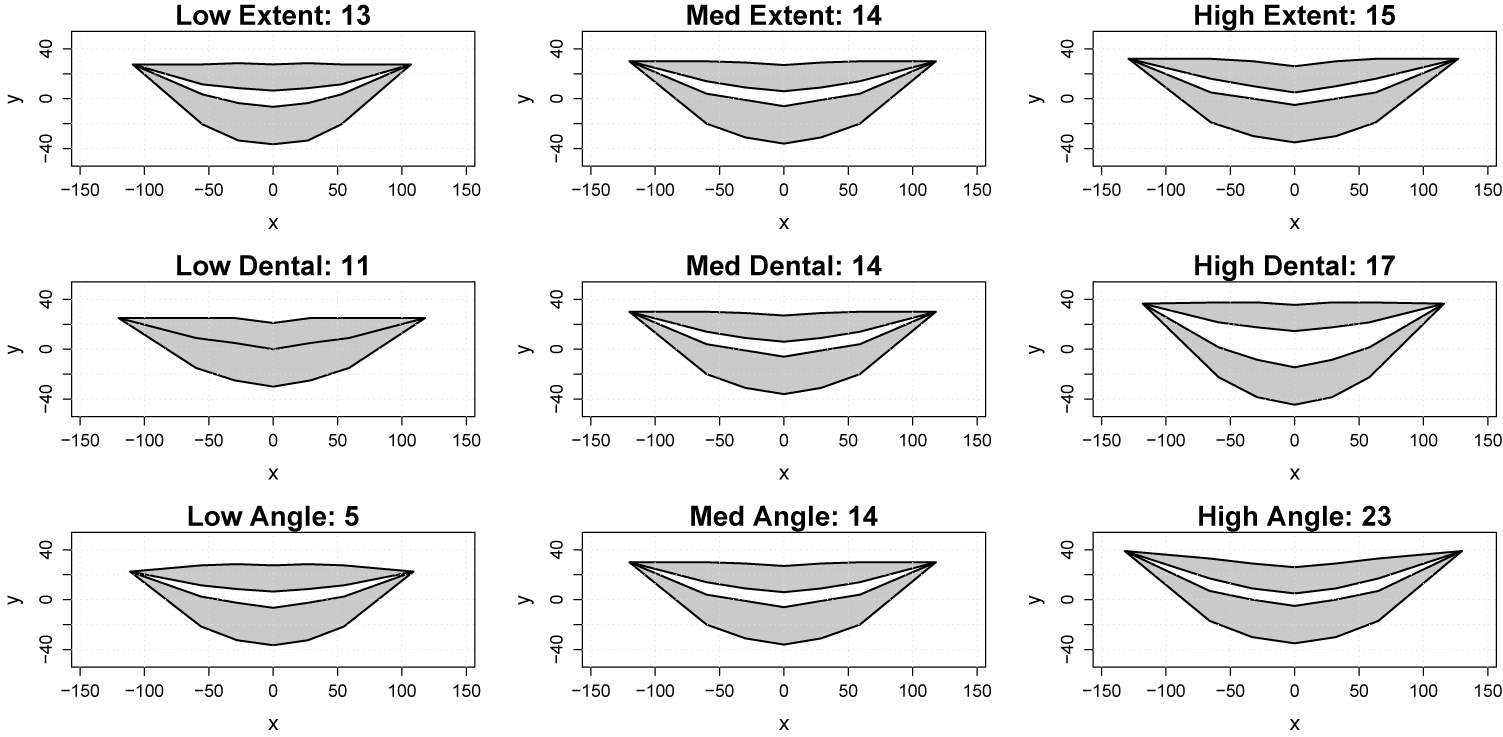
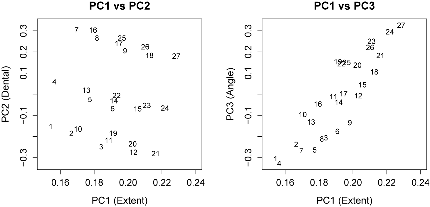
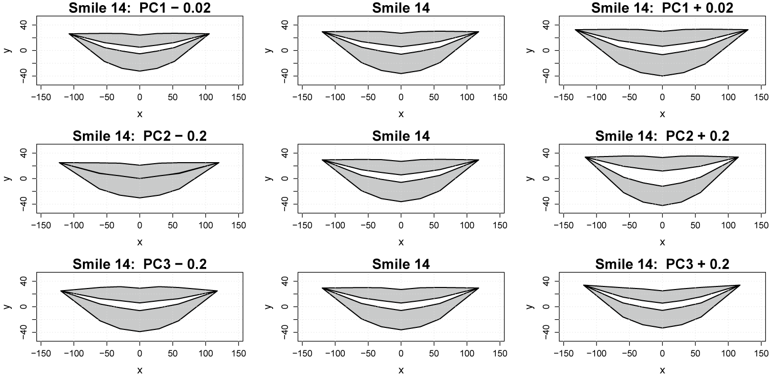
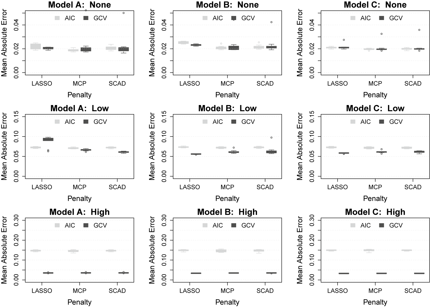
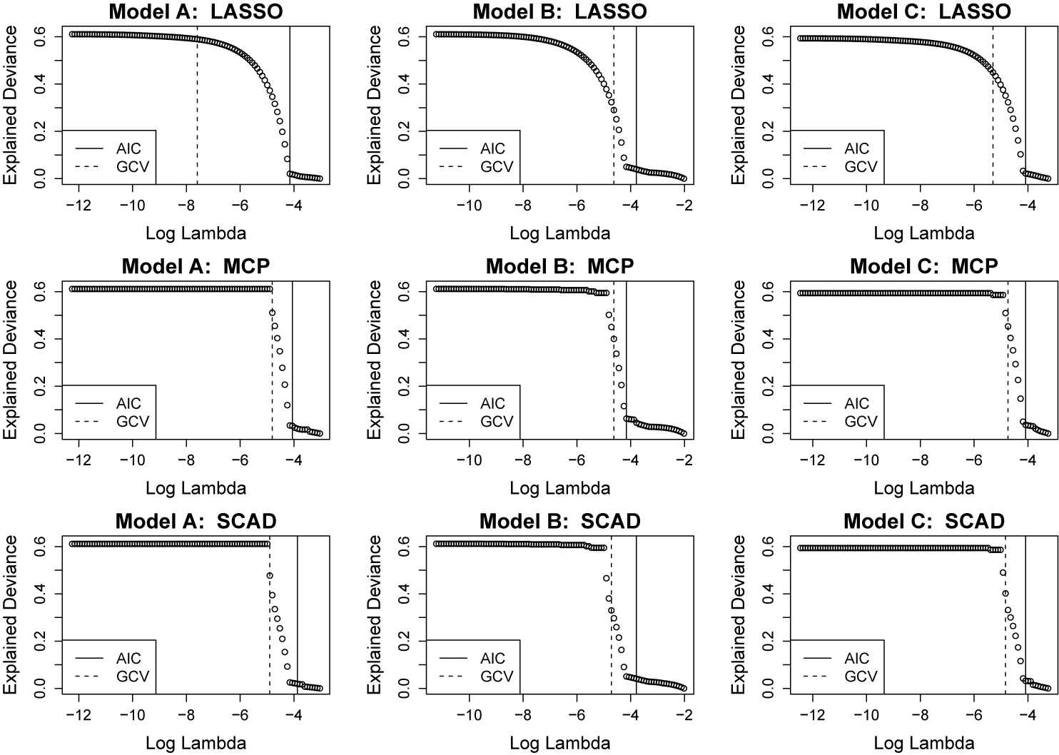

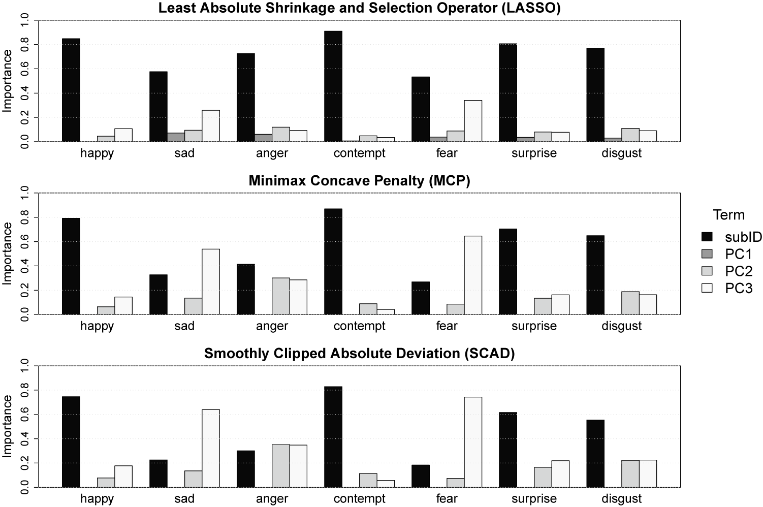
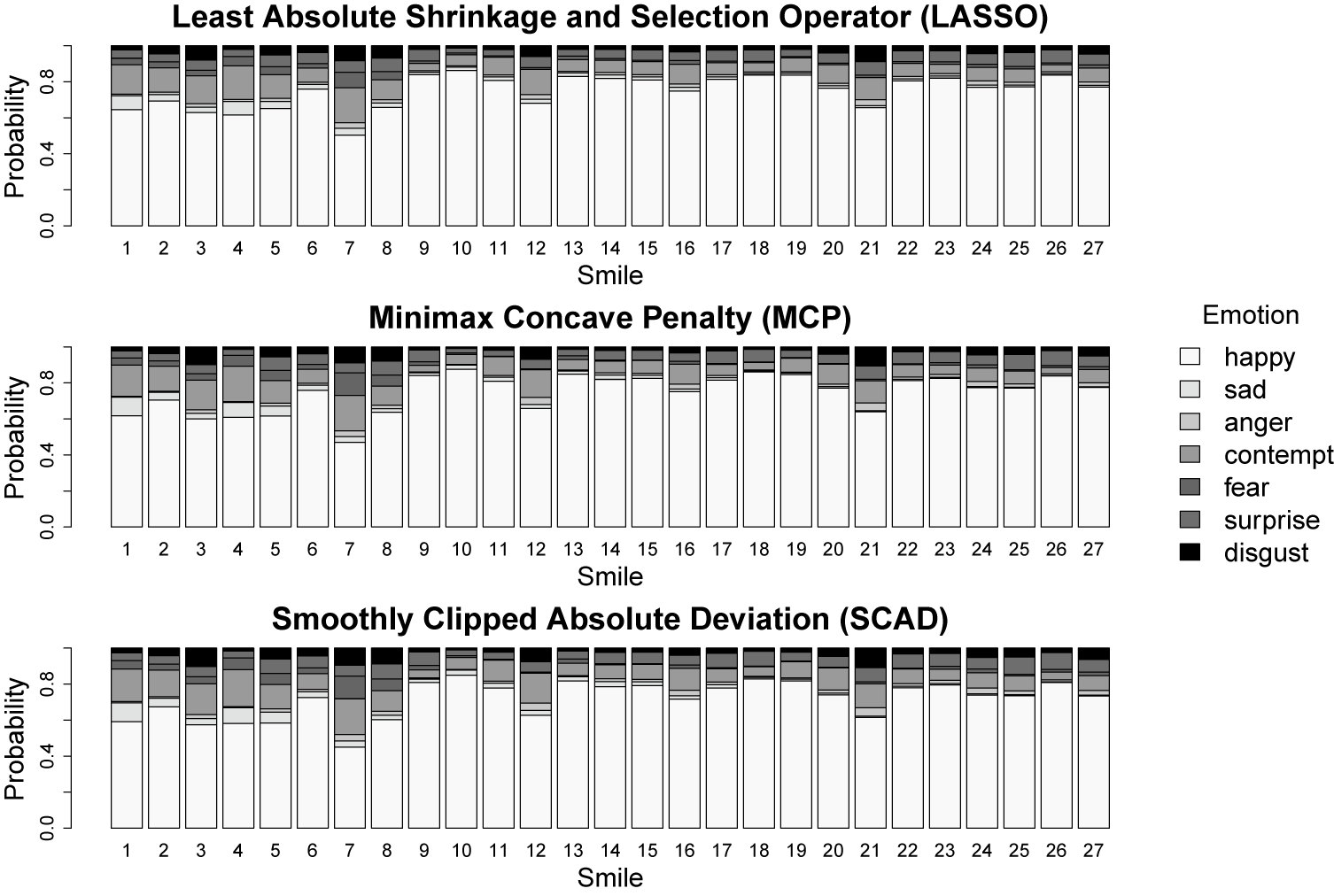
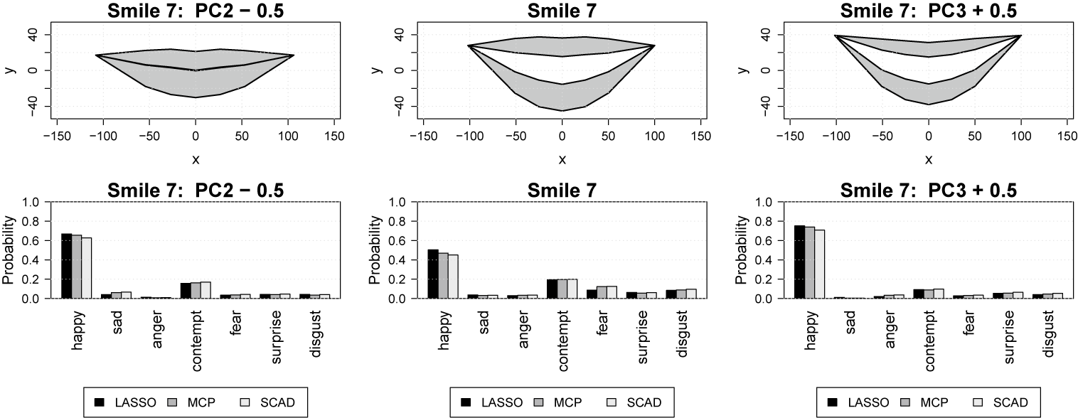
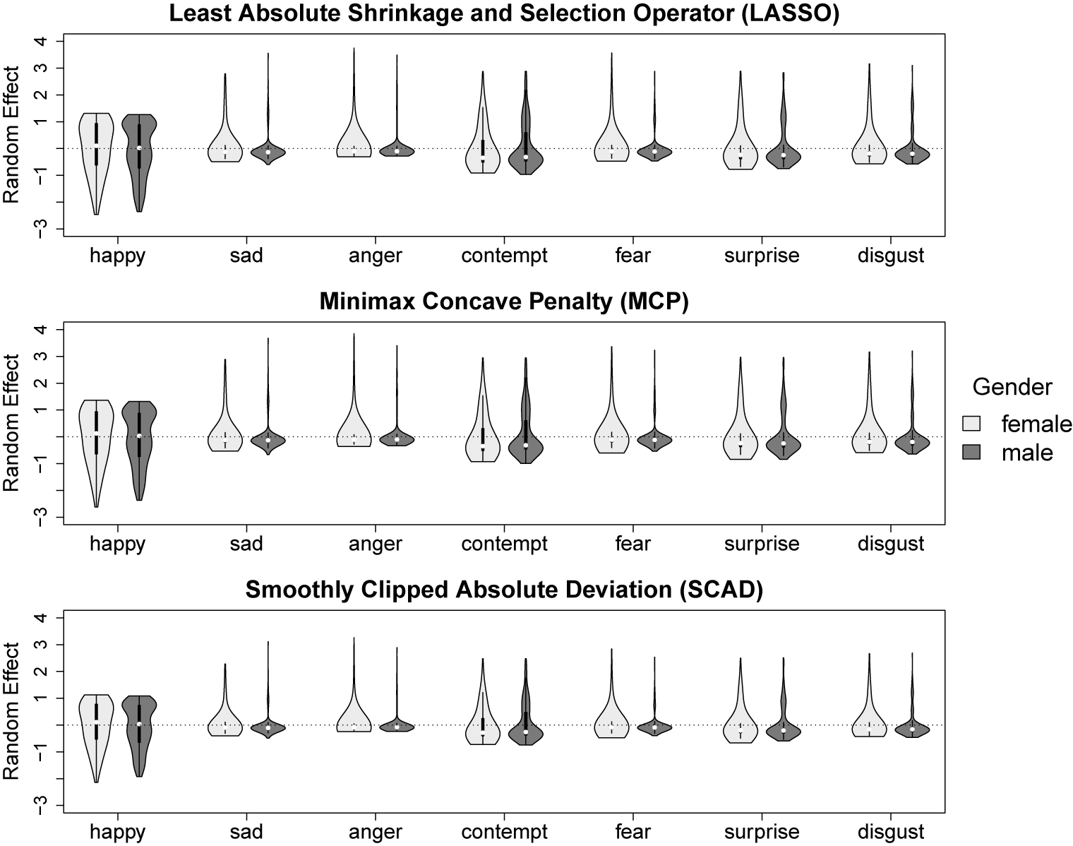


 Open access