

Introduction
Low-elevation glaciers and icefields are particularly sensitive to a changing climate. Thinning due to a negative surface mass balance can cause the ice surface elevation to lower and expose the ice to warmer climate conditions (Reference BodvarssonBodvarsson, 1955). Progressively larger areas of the glacier lie below the equilibrium-line altitude (ELA). If this effect dominates over the loss of ablation area due to retreat, the volume reaction timescale becomes negative and the glacier will disappear entirely (Reference Harrison, Elsberg, Echelmeyer and KrimmelHarrison and others, 2001), even under constant climate. This effect becomes even more pronounced if the ELA rises to higher elevations due to changing climate.
Many coastal glaciers in Alaska, USA, originate at low elevations and extend to sea level. The region has been identified as a significant contributor to global sea-level rise (Reference Arendt, Echelmeyer, Harrison, Lingle and ValentineArendt and others, 2002, Reference Arendt2013; Reference Berthier, Schiefer, Clarke, Menounos and RémyBerthier and others, 2010). Reference Larsen, Motyka, Arendt, Echelmeyer and GeisslerLarsen and others (2007) pointed out the large volume loss of lake-calving glaciers and identified Yakutat Glacier in southeast Alaska as one of the most rapidly thinning glaciers since 1948. During the past decade (2000–10) this glacier experienced a mean thinning of 4.43 m w.e. a−1, and its terminus has retreated 14.4 km during the past century (Reference Trüssel, Motyka, Truffer and LarsenTrüssel and others, 2013).
In addition to the negative surface mass balance, Yakutat Glacier also loses ice by calving into Harlequin Lake. Calving may enhance rapid retreat and could dynamically accelerate mass transport to lower elevations, causing increased thinning and thereby contributing to the mass-balance feedback described above. As glaciers around the world retreat into overdeepened basins, which they have often formed themselves by erosion, they leave behind proglacial lakes (Reference Warren and AniyaWarren and Aniya, 1999). Once terminating in such a lake, they change their dynamic behavior from land-terminating to lake-calving, which increases ice flow in the terminus area (Reference KirkbrideKirkbride, 1993). Despite the increasing number of lake-calving systems worldwide, these interactions have previously not been addressed in regional-toglobal glacier change assessments.
In this paper, we use a simplified model that includes surface mass balance, calving and glacier geometry changes, to evaluate the future volume loss of Yakutat Glacier. The model first calculates surface mass balance, adds volume loss from ice flux through the calving front, then adjusts the surface elevation of the glacier using an empirical elevation change curve and finally computes volume loss due to retreat of the calving front using a flotation criterion. Surface mass balance is calculated on a daily timescale; surface elevation adjustment and calving retreat are performed on a decadal scale. We consider the glacier evolution under two climate scenarios: one that is based on continued conditions as observed during the period 2000–10, the other a warming climate scenario that is based on predicted monthly temperature trends for the 21st century, as derived from a regional climate model. Our model allows us to predict glacier retreat and thinning without an ice-flow model, and is therefore computationally less expensive. Further, this approach can be applied to other retreating glaciers with limited measurements.
Study Area
Yakutat Glacier (342 km2 in 2010, based on our outline) lies on the western (maritime) side of the northern Brabazon Range in southeast Alaska (Fig. 1), 50 km east of the town of Yakutat, where the mean annual precipitation is 3576 mm a−1 (1917–2007; http://climate.gi.alaska.edu/climate/location/timeseries/Yakutat.html), making it the wettest town in the USA. Lake-terminating Yakutat Glacier is part of the low-elevation Yakutat Icefield with ice divides at ∼650ma.s.l., which is below the average ELA for this region (Reference Eisen, Harrison and RaymondEisen and others, 2001). This glacier presently has a very small accumulation–area ratio (AAR; e.g. 0.03 in 2007), and it experiences much higher thinning rates than the land-terminating glaciers of the icefield (Reference Trüssel, Motyka, Truffer and LarsenTrüssel and others, 2013).
Yakutat Glacier. The glacier is outlined in black; contour spacing is 50m (SPOT DEM 2010). Ice divides between Yakutat Glacier and other icefield outlets are shown in green. Massbalance stake locations are shown by red crosses. The weather station (YG) is located near the terminus and marked by a magenta diamond. Harlequin Lake is shown in blue. Coordinates are the UTM zone 8 projection. The inset shows the glacier location on a map of Alaska.
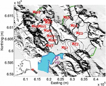
Yakutat Glacier calves into Harlequin Lake, which is >330 m deep in places and covered an area of 69 km2 in 2010, but is increasing its surface area due to the ongoing rapid retreat of the calving front. Radio-echo sounding (RES) measurements show that even at the highest locations, near the ice divides, the glacier bed lies below the current lake level (see ‘Ice thickness’ subsection below). Harlequin Lake is therefore likely to continue to grow and may eventually extend across most of the current glacier area as the glacier retreats, although unmapped ridges might divide the lake into several segments.
Data
To model the evolution of Yakutat Glacier, a digital elevation model (DEM) is required. Further, we use daily temperature and precipitation data at one location to calculate the surface mass balance of the glacier. Gridded monthly precipitation data are used to extrapolate precipitation across the glacier. The surface mass-balance model is calibrated using measured point-balance observations and volume change based on DEM differencing corrected for frontal ablation. Finally, to evaluate calving flux and glacier extent for each future decadal time interval, information on the ice thickness is required.
Digital elevation model
We use a DEM generated from Satellite Pour l’Observation de la Terre (SPOT) imagery (Reference Korona, Berthier, Bernard, Rémy and ThouvenotKorona and others, 2009), taken on 20 September 2010 and bias-corrected for the Yakutat Glacier area (Reference Trüssel, Motyka, Truffer and LarsenTrüssel and others, 2013). Grid spacing of the SPOT DEM is 40 m. The corrected DEM is used as the initial model input and to calculate the potential direct solar radiation for each day of the year (Reference HockHock, 1999).
Climate data
Our model relies on four different climate datasets: a short record of local temperature data; a longer record of temperature and precipitation from the nearest long-term station; gridded precipitation data; and projected regional climate data.
A weather station was deployed near (<1 km from) the terminus of Yakutat Glacier on bedrock (59°29′35.66″N, 138°49′22.94″W; 71 m a.s.l.; Fig. 1) and collected measurements from 16 July 2009 to 12 September 2011. Temperature data were recorded every 15 min with a HOBO S-THBM002 temperature sensor 2 m above ground and a HOBO U30 NRC data logger (for sensor and logger details see http://www.onsetcomp.com/). We refer to these data as YG data.
Daily precipitation and temperature data for the period 1 January 2000 to 31 December 2011 were downloaded from the weather station PAYA maintained by the US National Oceanic and Atmospheric Administration (NOAA, http://pajk.arh.noaa.govcliMap/akCliOut.php). PAYA is located at the airport (10ma.s.l.) in the town of Yakutat, 47.7 km northwest of the YG weather station. We refer to these data as NOAA data.
Monthly gridded (2 km) precipitation data for the period 2002–09 are obtained from Hill and others (in press). The data are based on re-gridded PRISM (Parameter elevation Regressions on Independent Slopes Model) monthly precipitation norms from 1971–2000, and are calculated from interpolated anomalies between measured monthly precipitation and monthly PRISM norms. Details are given at ftp:// ftp.ncdc.noaa.gov/pub/data/gridded-nw-pac/. Here we do not use those precipitation estimates directly. Rather we use the derived grid to spatially distribute measured, and appropriately scaled (via a multiplicative precipitation factor, p cor), NOAA data to the entire glacier grid. We only use winter data (October–April, 2002–09) to derive this grid, because solid precipitation occurs almost exclusively in those months, and the liquid precipitation does not enter our mass-balance model. Thus, the PRISM grids are used to describe spatial variability, while NOAA data provide temporal (daily) resolution.
Projected regional climate data are extracted from simulations from one of the Coupled Model Intercomparison Phase 5 (CMIP5) simulation experiments, which was generated by the Community Climate System Model 4 (CCSM4; Reference GentGent and others, 2011) under radiative forcing of the representative concentration pathway 6.0 (RCP6.0), which is considered a ‘middle-of-the-road’ scenario. Results for 2006–2100 are dynamically downscaled to the Alaska region at a 20 km resolution grid with the regional atmosphere model Weather Research and Forecasting (WRF; Reference SkamarockSkamarock and others, 2008). The downscaling approach is the same as in previous work using Mesoscale Model version 5 (MM5, the predecessor to WRF) for regional downscaling of CCSM3 (previous version of CCSM4) simulations (Reference Zhang, Bhatt, Tangborn, Lingle and EchelmeyerZhang and others, 2007).
NOAA temperature data are used to extend the short YG data series to the period 2000–10. We compare YG data with NOAA data for the overlapping time period. The data motivate a bilinear transfer function (Fig. 2):
Daily mean air temperature measured at the NOAA weather station at the airport in Yakutat, AK (10 m a.s.l.), vs temperature measured close to the terminus of Yakutat Glacier (71 m a.s.l.). A bilinear function was used to fit the data (black solid line); RMSE1 and RMSE2 refer to the root-mean-square error of the bilinear fit for the left and right part of the bilinear curve, respectively.

The intersection point (T 0 = 1.5°C) was picked based on minimal root-mean-square errors (2.14 for T NOAA < T 0 and 1.33 for T NOAA ≥ T 0). We apply this transfer function to the full NOAA record, thus providing a longer time series for the YG data location to run the glacier model.
This paper explores two trajectories for future climate. For scenario 1 (constant climate), we create a time series using the corrected NOAA temperature and the scaled and distributed NOAA precipitation data (2000–10). We then apply this 10 year record repeatedly until 2110. Repeating the decadal record allows us to conserve extreme temperature and precipitation events and preserves the observed variability over the past decade without a longer-term trend. We use this scenario to explore the magnitude of the mass-balance feedback due to surface lowering and the expected glacier change, without any further trends in climate.
For scenario 2, we calculate monthly linear trends from projected regional climate data over the 21st century, which are extracted from a dynamically downscaled CMIP5 simulation and are based on monthly means. We superimpose these temperature trends on observed temperatures from 2000–10 to preserve variability on shorter timescales. Trends for each month are shown in Table 1. Pearson’s linear correlation coefficients are calculated, and linear correlation is found to be significant for each month at the 5% level or better; for most months at <1% level. Largest slopes, and therefore highest temperature increases, are found for June, followed by July, May and February. Increased June temperatures cause earlier melt onset. Overall, the predicted melt seasons will be more extended and warmer, as shown for the period 2090–2100 in Figure 3.
Monthly temperature trends, ![]() , extracted from dynamically downscaled CCSM4 and linear correlation coefficients. Data for the 21st century
, extracted from dynamically downscaled CCSM4 and linear correlation coefficients. Data for the 21st century
Daily mean air temperatures at the terminus of Yakutat Glacier 2090–2100. Blue: scenario 1 (constant climate); red: scenario 2 (warming climate). Note that scenario 2 is subject to trends that differ for each month according to Table 1.

Projected precipitation does not show significant trends for any month. We therefore do not adjust precipitation in the warming scenario.
Surface mass balance
Point-balance observations (Fig. 1 gives locations) are used to calibrate the surface mass-balance model. Data are available at 14 locations in 2009, 12 locations in 2010 and 13 locations in 2011. Each year the measurements were made in late May and early September. Winter point balances are derived from snow depth measurements in May. Spring snow density in this warm, maritime climate is assumed to be 500 kg m−3, and was found to be very close to that value in spot measurements. Due to high summer melt rates (>6 m at lower elevations), ablation was measured using wires drilled into the ice rather than the widely used technique of ablation stakes.
Surface mass balances measured at 15 stations for 2009– 11 are shown in Table 2 and Figure 4. These data do not strictly represent stratigraphic summer and winter balances, because significant melting can occur before and after the summer measurement period. However, in model calibration they are used over the same time period as the measurements. Note that the lowest station shows a less negative summer mass balance than other points at higher elevation. This is because the lower east branch was covered with moss and other small dirt piles in the vicinity of this station, which appears to have an insulating influence on the ice.
Surface mass-balance measurements 2009–11. Summer balances are for the period given; values in parentheses refer to winter balances at the start of each period. Station names starting with E and W were located on the east and west branches of Yakutat Glacier, respectively. Elevation is the WGS84 height above ellipsoid of the 2010 surface
Measured balances over time periods specified in Table 2. Circles show winter balances estimated from snow depth. A value of 0 indicates a snow-free site at the time of measurement. ‘2008/ 09’ refers to winter 2008/09 and summer 2009, etc. Crosses show summer balances.

Ice thickness
The distribution of ice thickness on Yakutat Glacier is calculated using the method of Reference Huss and FarinottiHuss and Farinotti (2012), who use surface mass balance to estimate a volumetric balance flux and then derive ice thickness through Glen’s flow law (Fig. 5a). These simulations are calibrated with ground-based RES data that were collected on 19–20 May 2010 along several profiles on the upper west branch of Yakutat Glacier with a ski-towed low-frequency RES system. Errors in bed returns are influenced by uncertainties in wave propagation velocity, but dominated by the accuracy of the return pick, which we estimate at 0.1 μs, which corresponds to ∼8m. The mean difference between measured and modeled ice thicknesses along the center line is 25.1 m. Larger discrepancies occur mostly towards the glacier margins, where the glacier is shallower (Fig. 5b). We expect that these differences have little effect on our results, because incorrect ice thickness at the glacier margins will mainly result in differences in estimated glacier width. Ice thickness of the floating tongue was calculated from the surface DEM.
Modeled ice thickness (m) of (a) the entire Yakutat Glacier and (b) a subregion (rectangle in (a)) in the upper reaches of the western branch, based on Reference Huss and FarinottiHuss and Farinotti (2012). Circles mark the locations of radar measurements. Black circles indicate ice that is thicker than modeled, and white circles indicate shallower than modeled ice. Circle size scales with the magnitude of the difference and the scale of the difference is given at the bottom right. (c) Differences between radar measurements and modeled thickness along sampling track (sample numbers do not correspond to a constant distance).

Methods
The glacier model is made up of four steps. First it calculates the surface mass balance with daily resolution. Then each year’s volume loss due to calving, assuming a constant position of the calving front, is modeled and subtracted from the volume change due to the annual surface mass balance. Third, the combined glacier-wide volume change is converted into an elevation change for each gridcell, accounting for both changes due to surface mass balance and ice flow. Finally, for each decade, volume loss due to the retreat of the calving front is added.
Surface mass-balance model
We use the Distributed Enhanced Temperature Index Model (DETIM) to compute the glacier’s surface mass balance (Reference HockHock, 1999). DETIM is freely available at http://regine.github.com/meltmodel/. The model runs fully distributed, meaning that calculations are performed for each gridcell of a DEM. Melt, ![]() , is calculated by
, is calculated by

where M f is the melt factor (mm d−1 °C−1), a snow/ice is a radiation factor for snow or ice (mm m2 W−1 °C−1 d−1), T is the daily mean air temperature (°C) and I is the potential clear-sky direct solar radiation (W m−2). Equation (2) is an empirical relationship that was found to work well by Reference HockHock (1999). I is computed from topographic shading and solar geometry. Since this is computationally expensive, we keep the daily grids of I constant in time rather than recalculating I as the glacier surface evolves. Sensitivity tests with decadally updated radiation fields show negligible impact on our results.
DETIM is forced with daily climate data, and calculates surface mass balance for each glacier gridcell of a DEM. Temperature data at YG station are extrapolated to the grid using surface elevation and a lapse rate. Daily precipitation is adjusted by a precipitation correction factor and then distributed using a precipitation index grid (see above). Snow accumulation is computed from a threshold temperature of 0.5°C, that distinguishes between solid and liquid precipitation. Solid precipitation is added to the surface mass balance, whereas rain is not considered.
Five parameters are used to adjust the model to Yakutat Glacier: precipitation factor, p cor, temperature lapse rate, γ, melt factor, M f, radiation factor for ice,a ice, and radiation factor for snow,a snow. The precipitation factor, p cor, is a multiplier that scales the precipitation measured at the NOAA station, which is then distributed via the precipitation grid. γ describes temperature change with increasing elevation, and often varies between −0.45 and −1.00 × 10⁻² °C m−1 (Reference RollandRolland, 2003). M f, a ice and a snow are empirical parameters; the only limitation is that a ice must be equal to or higher than a snow, to account for generally higher albedo over snow than ice.
Calving
Calving flux, Q c (m3 a−1), is defined as the difference between the ice flux arriving at the calving front, Q, and the volume change due to terminus advance or retreat, R (here defined positive in retreat):
We first determine Q based on recent surface velocity observations (Reference Trüssel, Motyka, Truffer and LarsenTrüssel and others, 2013) and assume a steady terminus position (R = 0). The resulting volume loss is added to the volume change calculated by DETIM. The total volume change is then comparable with volume change as measured with DEM differencing, but not accounting for terminus retreat. In a later step, after the surface elevation has been adjusted, R will be determined. For simplicity, we ignore potential dynamical feedbacks after large calving events, such as speed-ups. This is justifiable because ice speed, and thus changes in ice flux to the calving front, are small compared with surface mass balance (Reference Trüssel, Motyka, Truffer and LarsenTrüssel and others, 2013).
Ice flux
For each decadal time step, we calculate ice flux at the terminus by assuming a spatially constant mean speed along the terminus of 74.3 m a−1 for the west branch and 30.0 m a−1 for the east branch, using results from a compilation of feature-tracked velocity fields between 2000 and 2010 (Reference Trüssel, Motyka, Truffer and LarsenTrüssel and others, 2013). The velocities are assumed to be temporally constant, although the flux will vary due to changing ice thickness. The ice speed is expected to be constant throughout the ice column, because the ice is assumed to be floating at the terminus and will therefore not experience resistance from the glacier bed. The flow direction is assumed to be along the center line, which is expected to remain constant for the future, as long as there is calving. We then identify the terminus by finding the ice-covered pixels that neighbor water, and find the flux, Q, by integrating the velocity, v, along the length, L, of the terminus:
where h is the ice thickness, and n is the unit normal vector to the line L. The ice flux correction is applied at time steps of 10 years, when the glacier DEM is adjusted (see below). Seasonal and interannual velocity variations are not considered, since their effect on the glacier surface elevation is assumed to be minimal.
Calving retreat
During the past century Yakutat Glacier was able to build and maintain a floating tongue for at least a decade, until the ice was sufficiently weakened by thinning, which allowed rifts to open and propagate, and caused large tabular icebergs to calve (Reference Trüssel, Motyka, Truffer and LarsenTrüssel and others, 2013). To address such a calving style in a simplified way, we apply a flotation criterion every 10 years to determine calving retreat. This flotation criterion is based on measured lake level, bed topography and ice thickness and allows floating tongues to disintegrate. Cells fulfilling the flotation criterion will transform from glacier cells to lake cells.
Surface elevation adjustment
In order to account for the surface mass-balance feedbacks due to retreat/advance and thinning/thickening, the DEM of the glacier surface must be adjusted, as changes in surface elevation and glacier extent expose the ice to different climate conditions. We determine the total decadal volume change (without calving retreat) by subtracting the ice flux through the calving front from the volume change from surface mass balance calculated with DETIM. We then use an empirical glacier-specific elevation change relationship, which includes dynamic components to redistribute the total volume loss (again without calving retreat), using a similar, but slightly modified, concept to that proposed by Reference Huss, Jouvet, Farinotti and BauderHuss and others (2010) and as outlined below. The resulting new surface elevation of the glacier is then used to compute retreat due to calving (see above) and retreat of grounded ice due to thinning. The latter is determined by glacier cells with a negative thickness, which are transformed into bedrock cells. The DEM is adjusted every 10 years.
Model description
Each gridpoint of the glacier experiences a rate of thickness change, ∂h/∂t, given by
where ![]() is the specific surface mass-balance rate (calculated by DETIM and converted to ice equivalent assuming a density of 900 kg m−3) and v
e is the emergence velocity. Because we have no information about v
e, we constrain the dynamic adjustment by observing that the glacier-wide rate of volume change,
is the specific surface mass-balance rate (calculated by DETIM and converted to ice equivalent assuming a density of 900 kg m−3) and v
e is the emergence velocity. Because we have no information about v
e, we constrain the dynamic adjustment by observing that the glacier-wide rate of volume change, ![]() , can be described as
, can be described as
where A is the glacier map area upstream of where the ice flux, Q, is measured. Observations show that elevation change, dz, is a function of elevation, f(z), and has a typical shape for each glacier with more negative dz at lower elevations (Reference Johnson, Larsen, Murphy, Arendt and ZirnheldJohnson and others, 2013). We assume that thickness change is equal to surface elevation change dz and this glacier-specific f(z) will shift up towards larger (less negative) mean ∂h/∂t during a period of colder climate, and down during warmer periods, so that
The shift, C, is obtained from the requirement that the integrated elevation change has to equal the total volume change:
and therefore

We thus find the surface elevation change, Δh, for each gridcell as a function of elevation:
The amount of shifting, C, is recalculated for each time interval (here 10 years), and provides a simple heuristic way of accounting for the dynamic adjustment of the glacier surface.
Elevation change curve
We use surface elevation change data from DEM differencing for the period 2000–10 (Reference Trüssel, Motyka, Truffer and LarsenTrüssel and others, 2013) to find the typical z − dh curve shape for each branch of Yakutat Glacier separately (Fig. 6). We fit both quadratic and exponential functions to the data. The root-mean-square error (RMSE) fits of both functions are nearly identical: ∼0.87 m a−1 for the west branch and ∼0.77 m a−1for the east branch. We prefer the exponential function because the quadratic fit extrapolates to increasing thinning at the highest elevations of the west branch. Both functions are simple empirical fits and do not have an obvious physical basis.
Elevation vs elevation change (dz − z) from DEM differencing (2000–10) with exponential and quadratic fits for (a) the east branch and (b) the west branch of the glacier.

This elevation change curve works well for thinning glaciers. However, for glaciers with a positive mass balance, the glacier would only thicken in the upper areas, unless the mass balance was sufficiently high to make Δh positive everywhere. Even in that case, the glacier would grow preferentially at high elevations and become increasingly steeper, advancing only slowly. Further, this approach cannot be used for dynamically complicated glaciers, such as surge-type glaciers. Most importantly, the approach outlined here does not allow a glacier to reach a new steady state. Despite all these caveats, we propose this approach here to simulate the observed continued thinning, even at the glacier’s highest elevation. Reference Huss, Jouvet, Farinotti and BauderHuss and others (2010) suggest a scaling approach, where the typical elevation change curve is not shifted vertically, but multiplied by a scaling factor. This requires us to fix elevation change to zero at the highest elevations, in which case we would not be able to reproduce the observed thinning there.
Calibration
We calibrate the model by adjusting the following parameters: precipitation factor, p cor; lapse rate, γ; melt factor, M f; radiation factor for ice, a ice, and snow, a snow. We perform a grid search for these parameters, run the mass-balance model and compare the results to two types of observations: seasonal point-mass balances measured over different time periods between 2009 and 2011 (Table 2) and total glacier mass change due to surface mass balance derived from DEM differencing between 2000 and 2010. The DEM differencing results are corrected for a calving flux derived by Reference Trüssel, Motyka, Truffer and LarsenTrüssel and others (2013), to make them directly comparable with the glacier-wide surface mass balance.
To find parameter combinations that provide good fits to the data (DEM differencing and point balances) we define a grid and systematically vary all five parameters over physically plausible ranges. First, we require that the 2000–10 cumulative surface balance matches the measured and flux-corrected DEM difference to within an area-averaged value of 0.1 m w.e.a−1. This value comes from an error estimate that is largely based on uncertainties in ice flux into the lake. The volume to water-equivalent conversion from DEM differencing was derived assuming a density of 900 kg m−3, based on the almost complete absence of a firn area on the glacier (Reference Trüssel, Motyka, Truffer and LarsenTrüssel and others, 2013). From the successful parameter combinations we then choose those that approximate all measured point balances best in a RMSE sense. This procedure is meant to primarily enforce a good fit to the 10 year geodetic balance, in order to better capture the long-term behavior and reduce systematic errors. The 15 best parameter combinations are then used to generate a range of predictions for the two climate scenarios. Figure 7 shows the range of the parameters found, and Figure 8 shows the fit to measured point balances for one of these parameter choices; others are similar. All parameter combinations lead to an underestimate of measured point balances. The reason for this is not clear, but we put a higher emphasis on matching the 10 year geodetic balance and accept this bias in matching point balances.
Ranges for the tested parameter combinations (black line). Circles indicate range where the most successful combinations were found. The quality of the fit increases with circle size and color (on a jet color scale, blue–green–yellow–red). Parameter values are in °C m−1 for lapse rate, γ, percent for p cor, mm °C−1 d−1 for the melt factor and mm m2 W−1 °C−1 d−1 for the ice and snow radiation factors.

Calibration of DETIM. Modeled point balance vs measurements from 2009–11 for the best-performing parameter combination (γ = −0.0065°C m−1, p cor = −40%, M f = 4.3 mm °C−1 d−1, a ice = 0.019 and a snow = 0.012 mm m2 W−1 °C−1 d−1 ). Balances are compared over the measured time period as given in Table 2.

As a final step we validate the model by applying the full model with dynamic corrections over the time period 2000– 10 and compare it with measured DEM differences (Fig. 9).
(a) Measured surface elevation change from DEM differencing 2000–10. (b) Modeled surface elevation change 2000–10. (c) Difference between measured and modeled surface elevation change. Note the different scale for (c).

Results
We first calculate the evolution of Yakutat Glacier under a constant climate (scenario 1). Figure 10a shows the ice thickness between 2020 and 2100 for one of the runs; others are similar. For all parameter runs, Yakutat Glacier will have lost >95% of its volume and surface area by 2100 and will vanish by 2110. Under a warming trend (scenario 2), the entire glacier will have disappeared by 2070 (Fig. 10b).
Evolution of Yakutat Glacier under (a) scenario 1 (2020–2100) and (b) scenario 2 (2020–60). The glacier has vanished by 2110 (a) or 2070 (b). Colors show ice thickness. Figure 1 shows a detailed current map.

We run the model with the 15 best-performing parameter sets (parameters: γ, p cor, M f, a ice and a snow) to explore the range of volume loss of Yakutat Glacier. Figure 11 shows the cumulative volume loss for both climate scenarios under all parameter runs. The initial volume is 115 km3 in 2010. The differences between the 15 cases are relatively small and represent the uncertainty due to parameter choice. The largest difference between models under constant projections is found in 2080, with a value of 3.6 km3, which corresponds to ∼3% of the original (2010) volume, but ∼27% of the mean 2080 volume. Under changing projections the largest spread in volume projections occurs in 2050, with a volume change difference of 3.4 km3. This also corresponds to ∼3% of the original volume or 19% of the 2050 volume. Towards the end of the model runs, the differences decrease again, because the glacier disappears entirely in all model runs. All parameter combinations predict a glacier-free landscape in the decade after 2100 under constant climate, and in the decade after 2060 in a warming climate.
Mean cumulative volume change for all 15 parameter sets (a) under scenario 1 (constant climate) and (b) under scenario 2 (warming climate). Volume change without calving is shown in red for scenario 1.
Discussion
Influence of calving
To assess the importance of calving to the overall volume loss we run the model without the calving module, hence assuming the glacier is land-terminating, and compare results with simulations that include calving (Fig. 11a). Results show that the greatest divergence occurs early in the model run: volumes in 2020 differ by 9.0 km3; this difference is reduced to 5.7 km3 by 2100. Without area loss from calving, the glacier would soon occupy a much larger area, +26 km2 by 2020 in scenario 1 (constant climate). This creates an artificially large surface area at very low elevation, which is exposed to high melt rates. That explains why the glacier would still be subject to very rapid volume loss, albeit at somewhat lower rates than if calving were occurring. The most important effect of calving is the glacier extent and appearance in its lower areas, as illustrated in Figure 12. It should be noted that a large part of the area loss predicted to occur by 2020 in this model has already taken place at the time of writing (summer 2014).
Difference in surface elevation in 2050 between a model run including volume loss by calving and a run excluding calving, i.e assuming the glacier was land-terminating. The model was forced by scenario 1 (constant climate).

Feedbacks
Glaciers are subject to two separate feedback mechanisms as they adjust their shapes to changing climate. First, as the ice surface continues to lower, the ice is exposed to higher temperatures, which in turn increases melt and thinning rates; a positive feedback mechanism known as the Bodvardsson effect (Reference BodvarssonBodvarsson, 1955) or the climate– elevation feedback. Second, as thinning rates increase, especially at lower elevations, the glacier reacts by retreating. By losing the area with the highest melt rates and reducing the ablation area, the glacier evolves towards a less negative mass balance. This is a stabilizing or negative feedback (e.g. Reference Harrison, Elsberg, Echelmeyer and KrimmelHarrison and others, 2001).
To investigate the relative strengths of the positive (surface lowering) and the negative (terminus retreat) feedback mechanisms on the glacier’s mass balance, we compare conventional mass-balance calculations with results where the surface elevation and geometry of the glacier are kept constant, known as the reference-surface mass balance (Reference Elsberg, Harrison, Echelmeyer and KrimmelElsberg and others, 2001; Reference Harrison, Elsberg, Echelmeyer and KrimmelHarrison and others, 2001). The latter excludes terminus retreat and thinning, and therefore neither of the feedback mechanisms influences the mass balance. The reference-surface mass balance is climatically more relevant, but does not describe the actual mass change of the glacier. Under a constant climate, it remains constant, and the cumulative reference-surface mass balance is therefore a linear function with time (Fig. 13a). Under a warming climate the reference-surface mass balance becomes more negative with time (Fig. 13b). For Yakutat Glacier during the first few decades after 2010 the conventional mass balance is slightly less negative than the reference-surface mass balance, indicating the effectiveness of the negative feedback mechanism. Similar observations were made by Reference Huss, Hock, Bauder and FunkHuss and others (2012) on 36 glaciers in the European Alps. The glacier maintains a relatively small mean thinning rate by retreating to higher elevations and thus losing area at low elevations. However, after a few decades, rapid thinning on the glacier can no longer be counteracted by retreat to higher elevations. The mean thinning rates will now continue to increase. This transformation is projected to occur around 2055 under scenario 1. In a changing climate, the glacier will react much faster and the reference-surface mass balance is more negative for the entire model run. Once the positive feedback starts to dominate, the volume loss of the glacier will quickly accelerate, even under a constant climate.
Comparison of specific reference-surface mass balance (blue) and specific conventional surface mass balance (red) for (a) scenario 1 and (b) scenario 2.

Under what climate conditions would Yakutat Glacier stop retreating?
The current glacier geometry and climate results in Yakutat Glacier having nearly zero accumulation area. We use our model to explore the scale of temperature or precipitation changes that would be necessary to return the glacier to equilibrium in its current shape. We run the 2000–10 model, systematically adding a temperature offset and a percentage change in precipitation, and analyze the resulting change in glacier-wide mass balance (Fig. 14). At current precipitation rates, the temperature would have to drop by 1.5°C to return the glacier to zero mass balance. At current temperatures, even a 50% increase in precipitation would not achieve a state of zero balance. Figure 14 shows that, in all likelihood, Yakutat Glacier has started an irreversible retreat, and the future temperature evolution will only affect the precise timing of the disappearance of the glacier.
Glacier-wide surface mass balance (m w.e. a−1) for mass-balance years 2000–10 calculated with DETIM as a function of temperature and precipitation changes applied to the original input data. The range of near-zero
![]() is highlighted in red.
is highlighted in red.

If a temperature decrease of 1.5°C is required to reach equilibrium in present conditions, an even larger temperature drop will be needed in the future, as the mean surface elevation of the glacier will be lower. The terminus will likely be at lake level for most of the glacier’s existence, because the glacier bed is near sea level, even at the ice divide. Equilibrium only appears possible when the glacier disintegrates into small high-elevation fragments.
Once the glacier retreats into a few small cirque glaciers, they can exist for decades, but they will be influenced by factors not incorporated into our model. First, thinning and retreat may be slowed by the influence of topography and location. Increased accumulation due to wind drift and avalanches may become important in the glacier’s mass balance (Reference DeBeer and SharpDeBeer and Sharp, 2009). Second, these small patches of ice will no longer be exposed to calving dynamics and losses.
We show here that climate conditions would have to change significantly in order to bring Yakutat Glacier into equilibrium. This raises the question of how this low-elevation glacier originated. Reference Trüssel, Motyka, Truffer and LarsenTrüssel and others (2013) hypothesized that, in addition to colder climate conditions, ice spilled over from adjacent Art Lewis and Vern Ritchie Glaciers, both of which have high-elevation accumulation basins, and served to initiate ice cover in the Yakutat Icefield. In addition, Nunatak and Hidden Glaciers (both glaciers of the Yakutat Icefield) thickened as a result of nearby Hubbard Glacier damming Russell Fiord, and ice from these glaciers helped Yakutat Glacier to grow.
Influence of lacustrine dynamics
Large-scale glacier collapse, such as that projected here, has been observed previously in Glacier Bay (Reference Larsen, Motyka, Freymueller, Echelmeyer and IvinsLarsen and others, 2005), only a few hundred kilometers south of Yakutat Glacier. Glacier Bay was primarily occupied by tidewater glaciers, and calving could have played a more prominent role in the rapid retreat and thinning. Large calving fluxes would have quickly lowered the mean ice surface, leading to reduced surface mass balance, and thus exacerbating the retreat in a similar mechanism to the one invoked here.
Many coastal glaciers in Alaska are lake-terminating at present. With current retreat rates, the number of such lacustrine systems will increase in the near future and some of these glaciers may experience similar rapid retreat and thinning to what we project here. As shown by Reference Trüssel, Motyka, Truffer and LarsenTrüssel and others (2013), Yakutat Glacier is exposed to the highest thinning rates (attributed to calving dynamics) of the Yakutat Icefield. Therefore, the formation of a proglacial lake is important for two reasons: (1) a previously land-terminating glacier will change its dynamic behavior into a lake-calving system with highest ice speeds at the terminus and (2) the terminus area will remain at lake level, where the ice surface will be exposed to higher air temperatures (similar to the description of water-terminating glaciers by Reference MercerMercer, 1961).
Finally, temperatures in the proglacial Harlequin Lake are currently very low (<1 °C, unpublished measurements by the authors). It can be speculated that a larger lake would be warmer due to an increased influence of solar radiation. It is conceivable that this would lead to increased rates of subaqueous melting and hence mass loss.
Conclusions
To predict future retreat and thinning of Yakutat Glacier, we combine a surface mass-balance model with a dynamic correction, include a simple calving law and adjust the glacier surface after each decade. This simple model of glacier evolution could be widely applicable to other retreating glaciers, although dynamically more complex glaciers (e.g. advancing or surge-type glaciers) will require a different treatment for dynamic adjustments. The dynamic adjustment allows for climate/glacier feedbacks. Two competing feedback mechanisms are known: a negative one due to glacier area loss at low elevations and a positive one due to surface lowering. Our model results show that, in the case of constant climate, these two feedbacks are of about equal strength for the next few decades, after which the positive feedback dominates. In the case of a warming climate, the positive feedback dominates for the entire model run. This is manifested by a conventional mass balance that is lower than the reference-surface mass balance.
Yakutat Glacier demonstrates that a low-elevation glacier is particularly sensitive to change. Even under present climate conditions, the glacier will retreat and thin substantially, by 2100 <5% of its initial volume of 115 km3 in 2010 will remain and by 2110 it will have disappeared. When forcing the same model with warming climate projections, the entire glacier is expected to disappear in the decade after 2060.
To prevent such a collapse, air temperatures would have to become much lower (by 1.5°C) or precipitation would have to increase by >50%, both unrealistic conditions. Our results show that Yakutat Glacier is far from equilibrium and will not transition back to steady state in the near future, even without any additional warming. Alaska has a number of other icefields that are of relatively low elevation. These and many low-elevation glaciers around the globe will experience similar scenarios.
Acknowledgements
We thank David Hill for providing gridded precipitation data. The downscaled climate data were generated under support of US National Science Foundation (NSF) award EAR-0943742. We thank Chris Larsen and David Podrasky for discussions, which helped to improve the manuscript. Andreas Vieli, Peter Jansson and the Scientific Editor, Bernd Kulessa, reviewed the manuscript and provided many suggestions that helped improve the presentation of the material. The SPOT 5 images used for DEM differencing were provided by the SPIRIT program (CNES). Funding was provided by NSF-OPP (grant ARC 0806463), and R.H. acknowledges funding from NSF EAR 0943742 and NASA NNX11 AF41 G.


