


1. Introduction
During and after the Second World War there was a period of extended rationing in neutral countries, such as Ireland and Sweden, as well as in participants in the conflict, such as the UK and the US. Despite the differences in attitudes of these countries with respect to the War (Harrison, Reference Harrison1998),Footnote 1 consumers were affected in similar ways: real household income rose over the war years in three of these countriesFootnote 2 but consumers were severely restricted in what they could spend their money on. While this regime was in place, whether for precautionary motives, or to postpone expenditure until the goods that households sought became available, there was a major increase in household saving. As the War came to an end in 1945, the precautionary motive for saving largely disappeared and, as the goods previously rationed gradually became more freely available, the household sector returned to more ‘normal’ consumption patterns and ran down some, but not all, of its stock of excess savings.
It remains to be seen whether the current crisis will see a similar pattern of behaviour (Romer, Reference Romer2021). Certainly, the restrictions on consumer behaviour are similar to the Wartime years, though on this occasion it is largely services that have been severely restricted. However, some studies already point to the exceptional savings motivated by the crisis (Ercolani, Reference Ercolani2020; Ercolani et al., Reference Ercolani, Guglielminetti and Rondinelli2021; NIESR, 2022). As yet, it remains unclear whether households’ exceptional level of savings is due to precautionary motives or because the services they would previously have purchased were temporarily unavailable. As populations became fully vaccinated, this could have provided a similar cathartic moment to the end of the War in Europe in May 1945. While there is evidence of a return to more normal consumption patterns in late 2021 and early 2022, the war in Ukraine and the related inflationary surge will probably limit the rundown in exceptional savings.
By applying a two-stage model, we estimate the extent of the ‘excess’ saving and the extent to which rationing constrained consumption in the War years. Subsequently, we measure the extent to which ‘dissaving’ contributed to the post-war consumer boom. Further, we show that some of the excess savings built up during the war years were subsequently channelled into the housing market, resulting in a rapid rise in prices, not only in the UK where some of the housing stock had been damaged by the War, but also in the other countries where no such damage occurred.
Section 2 describes the rationing regimes and the development of incomes and consumption during the War years in the four countries. The data sources are set out in Section 3. A model of consumer behaviour is described in Section 4 and this model is estimated in Section 5. Using this model, the effects of the War and rationing on consumer behaviour are quantified in Section 6, and conclusions are reached in Section 7.
2. Background: War, rationing and consumption
In this article, we do not consider countries, which endured wartime devastation and suffered a dramatic fall in output and incomes by the end of the War. In such countries, personal savings were wiped out and repairing the physical damage done by the War pre-empted private sector resources in the immediate post-war years. Instead, we consider four countries where the War severely disrupted the supply of consumer goods, both in terms of domestic production and imports, but whose productive structure was still functioning at the end of the War and where real household income in 1945 was at or above its pre-War level. Ireland and Sweden remained neutral while the UK and the US were active participants in the War.
During the War, a wide range of goods were no longer available in both neutral and belligerent countries. Part of the reason for the reduced supply was the reorientation of domestic economies to war-time production: for example, the Industrial Mobilization Plan in the US accounted for substantial economic activity in the national economy between 1940 and 1945. However, this increase in output was primarily focused on material required to prosecute the War (Jaworski, Reference Jaworski2017). Another important factor disrupting the availability of consumer goods was the exceptional difficulties in transport to Europe and within Europe. This is reflected in the dramatic fall in the consumption of affected goods in each country, as illustrated in figure 1.
Index of volume of consumption, 1938 = 100
Source: A detailed description of the sources of the data used is provided in Supplementary Appendix 2. The data are taken from the National Accounts for each country.

Figure 1 shows a steep fall in the volume of consumption in Ireland, Sweden, the UK and the US across a range of different categories of goods. Although the patterns of consumption differ from country to country, the sharp decrease in consumption of clothing and ‘other goods’ was common to Sweden, Ireland and the UK.Footnote 3 For the US, there was a major decline in the consumption of durable goods. Despite the similarities, each country suffered their own experience of shortages: whereas Ireland shows a major fall in the volume of fuel and power consumed, Sweden’s experience differs due to its vast resources of firewood and mineral products (Kander et al., Reference Kander, Malanima and Warde2014). In the UK, a food importer, there was also a substantial fall in the volume of food consumption.
The severe restriction of imports was reflected in rationing across a very wide range of consumer goods in all four countries. The most obvious shortage was in motor vehicles (included in the category ‘other goods’ or durables), where production and imports for personal use were suspended for the duration of the War. However, food rationing was also severe in the UK, but less so in Sweden. In the US and Ireland, major food producers, food rationing was also in place, but it imposed significantly fewer constraints than in the case of the UK. Details of the rationing regimes in each of the four economies are outlined in Supplementary Appendix 1.
In Ireland, the goods that were in very short supply and heavily rationed were fuel and power, clothes and other goods, all of which saw a very big fall in volume during the War years. Initially, in 1939 the government attempted price control measures. However, these measures proved ineffective. As described by Bryan (Reference Bryan2014), rationing of petrol began in 1939 and was gradually extended to other goods. Rationing of fuel and power was particularly severe, as Ireland was dependent on imports for all coal and oil. Rationing became particularly restrictive across a wide range of goods in 1942. When the War ended in 1945, the system of rationing was gradually unwound.
Rationing in the UK began in 1939 and was steadily tightened, with the toughest restrictions introduced in 1943 and 1944 (Zweiniger-Bargielowska, Reference Zweiniger-Bargielowska2000). Food was subject to strict rationing from the beginning of the War. The severity of the rationing policy was depicted by Broadberry and Howlett (Reference Broadberry and Howlett1998) as the government aiming for victory ‘at all costs’. While the War ended in 1945, rationing continued across a broad range of goods in the immediate post-War years. The rationing of clothing persisted until 1949Footnote 4 and rationing of a limited range of other goods ceased as late as 1954.Footnote 5 This continuation of rationing after the War partly reflected a priority for the UK to manage domestic demand in an economy with a historically high foreign debt burden and a binding balance of payments constraint. It also reflected the Labour government’s view that rationing constituted a ‘fair’ mechanism for protecting those on low incomes (Zweiniger-Bargielowska, Reference Zweiniger-Bargielowska2000).
As a neutral country, at the outbreak of World War II, Sweden’s policy makers had the precedent of World War I from which they could draw lessons. The searing experience of food shortages in 1917 and 1918, and a changing approach to economic policy meant that the government was expected to take a much more active role in managing crises in the 1940s (Schön, Reference Schön2010, p. 311). Preparations for a conflict had been underway during the mid-1930s, though the first detailed national inventory count was conducted in December 1939, some months before the first rationing was imposed. Thereafter, such reports were produced on a quarterly basis until 1945 (SOU, 1952, p. 404).
In stark contrast to World War I, during World War II in Sweden a rationing system was initiated within the first year of hostilities. Clothes and other goods were subject to relatively severe rationing and, while many food products were also rationed, shortages were much less severe than in the First World War. The large fall in the volume of alcohol sales in Sweden during the War was due to a major policy change that raised the price of alcohol. Unlike the case of Ireland, the Swedish energy supply was less constrained, with the exception of oil products. For many products rationing ended in 1945, while rationing of the last restricted item, coffee, concluded on 18 August 1951 (SOU, 1952, p. 403).
The situation in the US was very different. Contemporaries described the economy, which grew at a remarkable rate in the period to 1945, as a ‘production miracle’, which reversed the downward trends set in motion during the Great Depression (Rockoff, Reference Rockoff1998). Despite the huge productivity of the United States, consumers were still affected by restricted supply of consumer goods, as the requirements of the War economy were prioritised over personal consumption. Rationing began early in 1942 and continued until August 1945 (Brunet, Reference Brunet2021; Fishback and Cullen, Reference Fishback and Cullen2013). Rationing covered many food items, petrol, cars and tyres and a range of other goods.
Thus, the shortages and rationing affected the four economies over slightly different periods, partly reflecting when they entered the War (the UK in September 1939 and the US in December 1941), as well as the proximity and the severity of the conflict within Europe. Generally, rationing became seriously restrictive in 1941 and 1942, reached a peak in 1943 and 1944 and began easing in late 1945.Footnote 6 While rationing was phased out quite rapidly after the end of the War in the US, Ireland and Sweden, it persisted into the 1950s in the UK.
Across the four countries, the result of the restrictions on imports and the reallocation of domestic production to meet War needs, meant that there was a substantial change in relative prices. Specifically, the price of both imported goods, and those goods for which domestic production was restricted, rose relative to the price of food and services.Footnote 7 This also contributed to a substantial reduction in consumption of non-food goods.
Reflecting on the war-time experience, Tobin (Reference Stone1952) suggested that many of the objectives of the rationing regime could have been met more efficiently by other mechanisms. However, he concluded that:
Finally, the individualistic approach of the theory of consumer choice and of welfare economics may well obscure social effects of rationing of much greater importance than the effects which our atomistic theory discloses. For example, the feeling of sharing equally in an emergency situation may be more important for production and welfare than the individual incentives and choices on which economic analysis has traditionally centered.
As shown in figure 2a, real personal disposable income at the end of the War was slightly higher in Sweden and Ireland than it had been in 1938, significantly higher in the US and unchanged in the UK. Under normal circumstances the rise in real personal disposable income would have resulted in a rise in consumption of all categories of goods. However, there was also a dramatic rise in the personal savings rate (figure 2b). As shown in figure 1, when the rise in relative prices was combined with the effects of rationing, despite generally higher incomes, there was a very large fall in consumption of rationed goods.
(a) Real personal disposable income, 1938 = 100. (b) Personal savings rate. (c) Household currency and deposits (per cent of disposable income)
Note: The data for Ireland are for all sectors, not just households.
Source: A detailed description of the sources of the data used is provided in Supplementary Appendix 2. The data for (a,b) are taken from the national accounts for each country and the data for (c) generally come from the national Statistical Abstracts.

With unchanged real incomes, one might have expected that consumers would, nonetheless, have adjusted their patterns of consumption in response to the change in relative prices. This would have materialised as a shift towards consumption of services and goods that remained in relatively abundant supply, away from consumption of other goods where the relative price rose or where there was rationing. While such a change did occur, households only reallocated a portion of their disposable income to more readily available foods and services. As shown in figure 2c, they also saved a substantial part of their income. This increase in savings was reflected in a substantial rise in liquid bank deposits. In the US and the UK, investment also took place in War bonds, a less liquid asset.
This rise in savings was, in the first place, driven by the extreme uncertainty that prevailed during the War years. While Ireland and Sweden were neutral, coming through the War with minimal damage to life or property, there was a real concern between 1939 and 1945 that they might be dragged into the conflagration. There was an obvious motivation in the US and the UK for precautionary savings due to the War. However, some of the saving appears to have reflected the lack of choice available to consumers. Rather than spend all their income on the goods and services that were available, they chose to save for a future after the war when the full range of goods would, ideally, become available at more reasonable prices (Brunet, Reference Brunet2017).Footnote 8
This would suggest that the traditional assumption of weak separability of consumer preferences between one period and the next did not hold. Saving took place, not just for precautionary motives or to provide for retirement, but also because of an expectation of a better future when scarce or high price goods would be much more freely available (relative prices would change).
The end of the War in May 1945 produced a rapid turnaround in outlook. The precautionary motive for holding the accumulated savings disappeared at the same time as restrictions on imports and rationing began to be eased in 1946. Because much of the excess savings were held in liquid form, they could be spent on consumer goods or used to fund investment in housing.
Both the US and the UK had very large debt burdens in 1946, accumulated as a consequence of the cost of fighting the war.Footnote 9 In theory, this debt burden, because it portended a higher tax take in the future, could have affected consumers’ behaviour after the War through Ricardian equivalence (Barro, Reference Barro1974). The prospect of higher taxes or lower public expenditure in the future to deal with the exceptional debt burden could have discouraged consumers from spending their accumulated savings.
However, in the case of Sweden, the debt/GDP ratio only increased from 21 to 49 per cent between 1938 and 1946 and in the case of Ireland it actually fell from 41 to 30 per cent. In addition, in these two countries there was a substantial balance of payments surplus over the War years, which saw a significant improvement in their net foreign asset position. Thus, consumers in these two countries need not have feared a future of much more stringent fiscal policy. Despite these differences in indebtedness, consumers in the four economies behaved in a similar manner after the War ended, suggesting that Ricardian equivalence did not play a major role in their behaviour.
The easing in rationing occurred earlier in Ireland, Sweden and the US than in the UK. As households ceased to make exceptional savings there was a boom in consumption. Additionally, some of the ‘excess savings’ accumulated over the war years were spent on the newly available goods, adding to the consumer boom. Another destination of these funds was the housing market, which resulted in substantial real increase in house prices. Thus, some of the excess wartime savings were eventually invested to provide for retirement, even if that had not been the original reason for their accumulation.
3. Data
The data for personal disposable income and personal consumption at current and constant prices come from early national accounts for each of the four countries. Details of the sources are provided in Supplementary Appendix 2. In the case of the UK and the US, data are available from at least 1930. For Sweden, they begin in 1931 and for Ireland they commence in 1938. In principle, these data are available as continuous series to 2019 but, as described later, the model is estimated to 1970.
The data for personal savings are derived by subtracting personal consumption from personal disposable income. However, because the series for personal income and consumption for each country have been linked at a number of years between 1930 and 2019, over time there is some drift, which makes the residually determined personal savings data implausible for the earlier years. However, the change in the personal savings rate from year to year within the sample period generally provides a reasonable measure of the trend in the underlying personal savings rate.
In the case of the Irish data, this problem with the residually determined savings rate was dealt with by linking the personal savings rates from different vintages of national accounts. For both the UK and Sweden, there are discontinuities in the series for personal disposable income, which also affects the savings rate. These discontinuities are treated in estimation using dummies. For Sweden, Ireland and the UK consumption data are disaggregated into six different categories of goods and services at current and constant prices, derived by linking data for different vintages of national accounts. The six categories are food, drink, clothing, fuel and power, other goods and services. For the US, continuous series for a three-way breakdown into non-durables, durables and services are available from the Bureau of Economic Analysis. In the case of the UK, the data for consumption and disposable income were taken from a Bank of England spreadsheet of historical data (Thomas and Dimsdale, Reference Thomas and Dimsdale2017). Sefton and Weale (Reference Sefton and Weale1995) provide continuous series for the UK for the components of consumption.
While the categories of consumption used here are not directly aligned with the categories of goods that were rationed in each country during the 1940s, they do allow the identification of the categories of goods where rationing or supply shortages were particularly binding.
4. Modelling consumer behaviour
In the standard approach to modelling consumer behaviour, households save to provide for a steady flow of income over their lifetime and to deal with possible future shocks to that income stream (Deaton and Muellbauer, Reference Deaton and Muellbauer1980; Friedman, Reference Friedman1957). In addition, individuals’ choice of how much to work, and therefore their income, is affected by preferences for consumption and leisure. These factors help determine household income in a given year, how much of that income is spent and how much is saved.
Obviously, the War gave rise to huge uncertainty for households, not just in nations that were at war, but also in neutral countries. This helps explain a major rise in savings for precautionary purposes. However, the wartime restrictions on the availability of a wide range of goods also encouraged households to save so that they could acquire the rationed goods when peacetime supplies resumed.
Unlike the recent pandemic period, when consumers were ‘rationed’ in their access to services, in the War years the rationing affected consumption of goods, especially consumer durables. Because durables are capital goods, and they depreciated over the War years, when rationing eased there was a pent up demand, not just for additional durable goods, but also to replace worn out household equipment. In the case of the pandemic, there is likely to be a more limited pent up demand for services not consumed during lockdown (Beraja and Wolf, Reference Beraja and Wolf2021).
In the standard approach to modelling the pattern of expenditure of households in any given year, household behaviour is assumed to be affected by their preferred total level of consumption, their tastes and the relative prices of the different goods and services available to them (Deaton and Muellbauer, Reference Deaton and Muellbauer1980). This gives rise to a two-stage modelling approach.
First, the overall level of consumption in a year is determined by a consumption function. Subsequently, the consumption of individual commodities and services is a function of total consumption and the relative prices of those goods and services. In such a model, if availability of some goods or services is affected by rationing, then the spending that would have been directed at the rationed good or service is spread over the available goods and services. However, during the War years, and again during the pandemic, such a model does not align with actual behaviour by consumers. In both cases there was a major rise in savings, and only some of the income that could not be spent on rationed goods and services was spent on available goods and services.
The standard approach to modelling consumer behaviour, set out above, assumes weak separability between consumer preferences in individual years: an expected change in relative prices in the future does not affect households’ pattern of consumption in the current year or their total consumption in that year (Deaton and Muellbauer, Reference Deaton and Muellbauer1980).
Under normal circumstances, households may not have well-formed expectations about changes in future relative prices. However, in the years of the Second World War, and again during the recent pandemic lockdown, consumers were heavily constrained in what they could buy. When constrained, the shadow price of the rationed good or service was much higher than the prevailing price. In both cases there was the expectation that, when rationing ended, consumers would be able to buy what they wanted at lower prices than the prevailing shadow price of rationed goods and services. Thus, there was an expectation of a future change in relative prices. Under these circumstances, many consumers, instead of spending as they would normally on a range of goods and services, saved to spend on rationed goods and services in the future when their choices would no longer be constrained (Brunet, Reference Brunet2021).
It is difficult to distinguish this type of saving (motivated by providing for future consumption of presently rationed goods) from saving for purely precautionary motives. One indication that some of the saving was due to the prospect of future changes in relative prices is that high savings rates continued into 1945 or 1946, even though the impending end to hostilities reduced the motive for precautionary saving. Because the consumer goods that they wanted were not yet available, they preferred to withhold their consumption until their preferences could be satisfied. Furthermore, the fact that the exceptional rise in post War consumption, involved dissaving, accompanied by greater expenditure on previously rationed goods, suggests that wartime savings arose from more than a merely precautionary motive.
The behaviour of consumers through the War years and its aftermath is captured in the following model:
A simple model of consumption:
 $$ c={\alpha}_0+\theta y+{\delta}_W{D}_w+{\delta}_P{D}_P, $$
where c is the log of consumption at constant prices, y is the log of real personal disposable income and DW and DP are dummies for the War years and the immediate post-War years respectively. The precise timing and definition of the dummies is given in Supplementary Appendix 2.
Household expenditure on individual goods and services was modelled using an Almost Ideal Demand System (AIDS) model (Deaton and Muellbauer, Reference Deaton and Muellbauer1982).
 $$ {S}_i={\alpha}_i+\varSigma {\beta}_{ij}\log \left(\frac{P_i}{P_j}\right)+{\beta}_i\log \left(\frac{Y}{P}\right)+{\delta}_i{D}_w+{\gamma}_i{D}_P. $$
Si is the share of expenditure on item i, Pi is the price of item i, Y is real consumption and P is an index of consumer prices. The share of expenditure allocated to each category of consumption is a function of the relative prices of the different commodities, of total expenditure at constant prices, and dummies, DW, to reflect the constraints on choice of consumer goods and services as a result of shortages and rationing during the war. In addition, after the War there may have been some catch up in expenditure of previously rationed goods, captured by a separate dummy DP. As suggested in Deaton and Muellbauer (Reference Deaton and Muellbauer1982), a Stone (Reference Stone1953) index for consumer prices P is used where:
 $$ \log (P)=\sum {S}_i\log \left({P}_i\right). $$
The two-stage model used here treats prices of individual goods and services as exogenous. As relative prices also changed due to wartime shortages, the model here does not capture the full effects of the War on changing consumption patterns, only the direct effects of higher savings and the effects of rationing and reductions in supply.
In the AIDS model, as theory would indicate, symmetry and homogeneity are imposed. Because the shares Si sum to unity, one of the equations is dropped in estimation. This means that the errors will be correlated across the equations. As a result, the AIDS model is estimated using the Seemingly Unrelated Regressions (SUR) estimator. As set out in Supplementary Appendix 3, a series of identities are appended to close the model.
As discussed earlier, linking series over longer time horizons poses problems. In addition, tastes and consumer preferences change over time and technical progress has typically resulted in the development of new products and services. Thus, while continuous series are available to 2019, the model is estimated using data that begin before the War, span the War years, and end in 1970. The start date for each country model depends on data availability for the 1930s.
5. Results
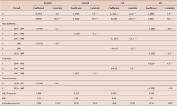
The results of estimating the simple consumption function, equation (1), are shown in table 1. Except for the US, the log of consumption was regressed on the log of real personal disposable income and a series of dummies.Footnote 10 For the US, consumption was regressed on real personal disposable income and dummies.
Results for consumption function equation (1)

*** Significant at 1 per cent level;
** Significant at 5 per cent level;
* Significant at 10 per cent level.
Because the War affected the different countries over different periods, the dummies are country specific. In choosing the appropriate span of years to include in the dummy, guidance was taken from the DFFITS statistic in the regressions without dummies, which pointed to observations that were exerting a significant leverage on the estimation results. Because the relaxation of constraints on consumption after the War affected each country differently, these dummies are, once again, country specific. Dummies were included in the equations for Sweden and the UK due to discontinuities in the data for real personal disposable income in 1947 and 1949, respectively.
In the case of each of the four countries, the elasticityFootnote 11 of consumption with respect to personal disposable income was significant, with a plausible coefficient close to but significantly different from unity.
In the case of Sweden, the serious impact of the War lasted from 1940 to 1944 and this is covered by one dummy, which is significant indicating that consumption was 5 per cent below normal. Consumption was especially low in 1943 at the height of the war, as reflected in a second significant dummy. Testing for a post-war boom fuelled by dissaving did not prove significant. As discussed earlier, there is a discontinuity in the personal disposable income data at 1949, reflected in the significant dummy covering the period from 1950 to 1970.
For Ireland, the War exerted a strong effect on consumption behaviour from 1941 through to 1946 with consumption also 5 per cent below normal, very similar to the other neutral country we consider, Sweden. However, once rationing was phased out, the significant dummy for the years 1947 and 1948 shows that there was an abnormally high level of consumption, reflecting some dissaving.
The US entered the War in December 1941. The dummy for the period 1942–1945 is significant implying a major reduction in consumption of over 20 per cent, despite rapidly rising real incomes. A second dummy is included for 1941, as it is clear that expectations of conflict, and the reorientation of the economy towards a wartime footing, was already affecting consumption and savings in that year. The significant dummy for the years 1947–1949 suggests that there was some limited dissaving in those years, helping fuel a consumption boom.
For the UK, as discussed by Broadberry and Howlett (Reference Broadberry and Howlett1998), the model suggests that the war years of 1940–1944 saw an exceptional reduction in the volume of consumption of 18 per cent, very similar to that observed in the other combatant, the US. This is not surprising, given that the UK was seriously impacted by the conflict in a way that the neutral countries were not. There is also evidence of a contribution to a post-war rebound in consumption from some dissaving, reflected in the positive dummy for 1946–1951.
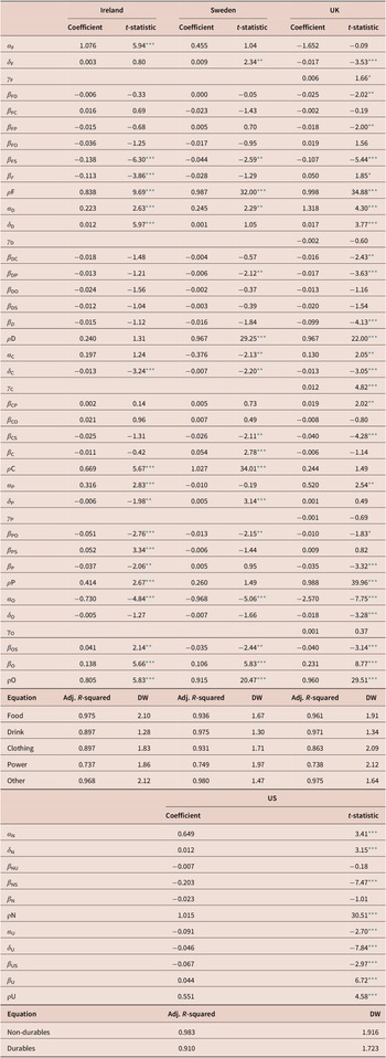
The AIDS model of consumer demand was estimated for the four countries. For the US, data were only available for a three-way breakdown of consumption. The results of estimating the model for the four countries are shown in table 2. All the equations have been adjusted for autocorrelation. A Wald test was conducted on the joint significance of the War dummies in each model. It decisively rejected the hypothesis that the coefficients on the wartime dummy were zero—that consumers’ behaviour was ‘normal’ in those years. For the UK, a post-war dummy for the years 1949–1951, when rationing was largely phased out, is also significant.
Estimation results of AIDS model of consumer demand

Note on the suffixes: C, clothing; D, Drink; F, food; N, non-durables; O, other goods; P, fuel and power; S, services; U, durables.
*** Significant at 1 per cent level;
** Significant at 5 per cent level;
* Significant at 10 per cent level.
In the models for the four countries, the dummies for the war years are significant for quite a number of categories of goods at least at the 5 per cent level: for Ireland for expenditure on drink, clothing and fuel and power; for Sweden for food, fuel and power and clothing; for the UK for food, clothing and fuel and power; for the US for both durables and non-durables. For the UK, the post-war dummy was also significant for clothing, implying that when rationing ended, there was a pent up demand for replacement clothing.
In the model for Ireland, the βi coefficients, which determine whether the income elasticity of demand is greater or less than unity, were significant for food and fuel and power (less than one) and other goods (greater than one). For Sweden, the βi coefficients for clothing and other goods were also significant, at least at the 5 per cent level. So too for the UK the coefficients for drink, fuel and power and other goods were significant. The βij coefficients which determine the cross-price elasticities were significant in a number of cases involving interaction between services prices and other prices.
Finally, for the US model, most of the coefficients were significant. One of two exceptions was the coefficient determining the income elasticity of demand for non-durables, which suggests an income elasticity not-significantly different from one. The wartime dummies suggested that consumption of non-durables was higher than normal while that of durables was significantly below normal, reflecting the rationing regime in place and the constraints on supply.
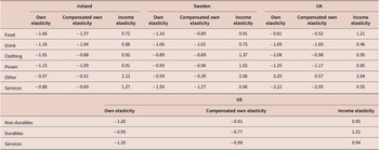
Table 3 shows the uncompensated and compensated own price elasticities and the income elasticity for each category of consumption for a representative year, 1948. The pattern of the elasticities is rather similar across all four countries implying similar consumer preferences. As is suggested by theory, with one exception, the compensated own price elasticities of demand are negative: higher prices see a fall in demand. The one exception is the UK own price elasticity for other goods which is positive.Footnote 12 Across the other three countries, the own price elasticity for other goods (durables) is lower than for the other consumption categories. The compensated own price elasticity for clothing is, in all cases, less than unity. For Ireland, the price elasticity for food is greater than unity, whereas for the other economies it is less than unity. In Ireland and Sweden, the income elasticity of demand for food was less than one, reflecting the fact that it was a necessity. Surprisingly for the UK, it is greater than unity and for the US, the income elasticity of demand for non-durables is also less than unity.
Elasticities for different categories of consumption, 1948

These results also indicate that the ‘other goods’ or durables category of consumption, which was heavily rationed in all three countries, had the highest income elasticity of demand, indicating that it was a ‘luxury’ good. As mentioned earlier, it also had a low own price elasticity of demand. Thus, without rationing prices would have had to have been exceptionally high due to the reduction in supply. In turn, this implies a very high shadow price for other goods during the War years across all four countries. For Sweden, clothing also exhibited a high-income elasticity of demand, and the negative war-time dummy reflects the effects of rationing.
6. Simulation results
The model outlined above, together with a set of identities to close the model, was simulated as a system for the four economies. First, the model was constrained to track the actual historical outcome by adding a set of fixes for each individual year in each of the endogenous equations. This provided a baseline against which to measure the effects of War-time precautionary saving, rationing and the relaxation of restrictions after the War.
The same model was then simulated setting the wartime and post-war dummies to zero in the equation determining consumption (and savings). The difference between this simulation and the baseline shows the impact on consumption and savings of the uncertainty about the future, giving rise to precautionary savings, and also the effects of saving accumulated to engage in future consumption of presently rationed goods. As well as affecting saving, the higher consumption in an unrationed non-War environment would have resulted in higher consumption of individual categories of goods.
In the final simulation, the War-time dummies (and the post-War dummies for the UK) were set to zero in the model of consumer demand and the difference between that simulation relative to the baseline reveals the direct effect of rationing on consumption patterns during the War years.
Figure 3 shows the actual savings rate and the counterfactual savings rate if there had been no precautionary savings, and no savings to provide for consumption in the future of currently rationed goods. The area between the red line (War) and the black line (no-War) represents the cumulative excess savings during the war. For neutral Ireland and Sweden, the exceptional personal savings represented a cumulative 30 and 28 per cent of personal disposable income respectively. For the US and the UK, both participants in the War, it represented 71 and 90 per cent of personal disposable income, respectively.
Effects of war on personal savings rate

If the sole motivation for saving during Wartime had been precautionary in nature, the bulk of the savings might have been spent in the aftermath of the War. As can be seen from figure 3, the significant post-war dummy in the equations for Ireland, the US and the UK indicates that a limited proportion of the build-up in exceptional savings was used to sustain an above average level of consumption after the War as goods, previously rationed, became available. However, the rundown in savings comprised only a small proportion of the build-up in household financial assets during the War years.
For Ireland and the US, the cumulative dissaving after the war came to between 6 and 7 per cent of personal disposable income. For the UK, the dissaving was spread over a longer period amounting to 15 per cent of personal disposable income. In each case, the cumulative dissaving was only a fraction of the savings actually built up during the War years.
Figure 4 shows the effects of excess wartime savings and rationing upon the consumption of goods in short supply: clothing and other goods for Sweden, Ireland and the UK and durables for the US. It shows how much higher consumption would have been without rationing and excess savings.
Effects of war on categories of consumption that were rationed

As can be seen for Sweden, without the effects of the War, the consumption of clothing would have been 13 per cent higher in 1940, and over 20 per cent higher in 1943. The effect of the excess savings in reducing consumption of clothing was slightly larger than that of rationing. The reduction in consumption of other goods was even greater at almost 30 per cent in most years and 40 per cent in 1943. With a higher income elasticity of demand, the increased savings rate had a big effect, proving more important than the direct effects of rationing and supply shortages.
By contrast, in Ireland the effect of excess savings in reducing consumption of clothing was dominated by the effect of rationing. In 1943 and 1944, without the War, consumption of clothing would have been more than 25 per cent higher than the War counterfactual scenario. For other goods, as in Sweden, because of the high-income elasticity of demand, the effect of excess savings was greater than the effect of rationing. Without the effects of the War on saving and supply, consumption of other goods would have peaked at around 40 per cent above War-time levels in 1943 and 1944 and would have been around 25 per cent higher in other years. The graphs also show that the exceptional dissaving in 1946 and 1947 meant that consumption of both categories of goods was higher than it would have been without the legacy effects of the War.
For the UK, the effects of the War were much bigger. Consumption of clothing would have been over 30 per cent higher in the early 1940s without the effects of the War. Over half this effect is attributable to the higher savings rate. In the case of other goods, the effects were even more dramatic. Consumption would have been 130 per cent higher in 1944 without the War. The major impact was attributable to the higher savings rate. As in Ireland and Sweden, with a very high-income elasticity of demand, the decision to save rather than to spend had a substantial effect on consumption.
The post-war dissaving contributed a small amount to higher consumption of these two categories of goods in the UK. The ending of rationing had a more marked effect on consumption of clothing as people restocked their wardrobes in 1949–1951. For the US, consumption of durables would have been 100 per cent higher in the absence of the War. The effects of rationing dominated the effects of the exceptional savings rate. As in the case of Ireland, there is evidence of a small effect after the War from dissaving, adding to consumption in the years 1947–1949.
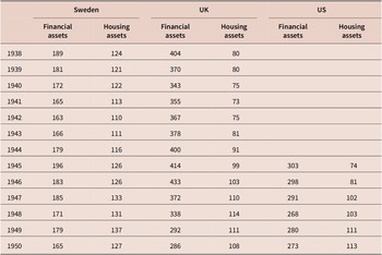
Instead of running down excess savings after the War, households in all four economies used a significant proportion of the exceptional increase in their financial assets to invest in the housing market. Table 4 shows household financial and housing assets as a percentage of personal disposable income. For Sweden and the UK, where data are available back to 1938, financial assets accumulated over the War years, reflecting the high rate of personal savings. However, after the War in Sweden, the UK and the US, financial assets fell as a share of income. In the case of the UK and the US, this was partly offset by an increase in assets held in the form of housing.
Household assets as a per cent of personal disposable income

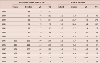
The result of this reallocation of financial assets to investment in housing was that in all four countries there was a substantial rise in real house prices (table 5). The biggest increase was in Sweden where prices had more than doubled by the end of the 1940s. In Ireland, by 1947 house prices were already 50 per cent above their 1945 level (Keely and Lyons, Reference Keely and Lyons2020). However, in the Irish case, a return to large-scale emigration quickly reversed the trend. The rise in house prices in the US and the UK was more moderate. In the case of the US, this was attributable to a more rapid supply response in the construction sector.
House prices and the rate of inflation

Source: See Supplementary Appendix 2.
Brunet (Reference Brunet2017) reports for the US that:
‘Nationally, home construction boomed after World War II (after being strictly limited during the war years). Construction of slightly more than 1 million new housing units began in 1946, compared to just 325,000 housing starts in 1945 and a pre-war high of 620,000 in 1942’. By 1950 housing starts in the US had reached 1,900,000 units, moderating the pressure on house prices.
Finally, while the wartime economy in Europe and the US gradually reoriented itself to produce the goods and services that post-war consumers desired, this took some time to accomplish. However, consumption patterns adjusted more rapidly and, as discussed by Mandelman (Reference Mandelman2021), the result was a temporary rise in the inflation rate in the US in 1947 and 1948 (table 4). A rather similar temporary rise in inflation was observed in Ireland and Sweden in those years. The fact that the UK had continued with rationing, partly to manage imbalances between supply and demand, did not prevent a similar temporary inflation surge there too. However, in all cases the positive effects on the inflation rate were short-lived.
7. Conclusions
The Second World War saw a substantial build-up in personal savings in Sweden, Ireland, the UK and the US. The rise in the savings rate occurred partly because of war-induced fears about the future, but also because consumers could not purchase many of the goods they desired due to rationing or scarcity. Instead of spending their incomes on what was available, households saved to spend in the future when the rationed goods returned to the market (Brunet, Reference Brunet2021). The rise in savings was particularly marked in the two countries that were participants in the War—the US and the UK. As a consequence of the rise in the savings rate, there was a dramatic fall in the volume of consumption during the war years in the four countries considered here (Sweden, Ireland, the UK and the US). This fall occurred despite the fact that real incomes were unchanged or were even higher in 1945 than at the start of the War in 1939.
In addition to the fall in the volume of consumption as savings rose, which would likely have resulted in a major reduction in the consumption of different categories of goods and services, there is clear evidence that rationing further reduced the consumption of key commodities, especially clothing and ‘other goods’ (consumer durables). When the War ended and rationing was gradually phased out, households returned to spending the majority share of their incomes. This inevitably resulted in a consumer boom. There is also evidence that some limited dissaving further fuelled the boom in Ireland, the UK and the US.
Nonetheless, this dissaving absorbed only a small share of the excess funds accumulated over the War years. Instead, a larger component of the excess savings was channelled into the housing market. The result was a rapid rise in real house prices between 1945 and 1948 in all four countries. The increase in house prices in the US was less pronounced than in Ireland and Sweden, due to a rapid supply response.
The Covid pandemic represents the first post-war event of comparable magnitude to World War II in terms of an exogenous shock, which has forced a reduction in consumption, in this case of services. Over the 2 year period 2020–2021, cumulative ‘excess’ savings built up by households represented between 12 and 14 per cent of personal disposable income in the US, the EU and the UK.Footnote 13 These savings are generally held in liquid form. While substantial, this increase in savings is still much smaller than the ‘excess’ savings that materialised in the War years in Sweden and Ireland (around 30 per cent), and only a fraction of the excess in the US and the UK over that period (between 70 and 90 per cent). Nonetheless, the build-up is the largest seen in recent decades.
It remains to be seen whether the rebound in consumption in 2022 and 2023 mirrors the post-War experience. Even with a return to a ‘normal’ savings rate, there would be a very big rise in the volume of consumption. If households behaved as they did during the post-War years, some of the excess savings may be used to further expand consumption. However, the Ukraine war and the rise in inflation could lead to a new bout of precautionary saving. In the past, high rates of inflation were associated with reductions in consumption (Davidson et al., Reference Davidson, Hendry, Srba and Yeo1978).
Also, while households were rationed in their purchase of goods, including consumer durables, during the War years, throughout 2020 and 2021 they were rationed in their consumption of services. Beraja and Wolf (Reference Beraja and Wolf2021) suggest a bigger response in a recovery from a recession that was biased towards cuts in expenditure on consumer durables than one where expenditure cuts were concentrated on non-durables and services.
Despite the uncertainty caused by the situation in the Ukraine, as in the period 1945–1948, more of the savings may find their way into the housing market, with significant implications for house prices. In 2021, house prices were already 15–20 per cent above 2019 levels in the EU and the US and a further unwinding of household savings could see continuing inflationary pressures in housing markets over 2022 and 2023.
Supplementary Materials
To view supplementary material for this article, please visit http://doi.org/10.1017/nie.2022.19.


 Open access