


1. Introduction
Recent advances in behavioral economics have shown that cognition is difficult and that this difficulty can lead to predictable divergences from classic economic behavior. Two areas that have found significant success in modeling such cognitive difficulties are rational inattention and strategic sophistication. Rational inattention proponents (beginning with Sims, Reference Sims2003) have shown that in decision-making settings, individuals acquire information in a way that maximizes the utility of gaining that information less the mental costs of doing so. In strategic settings, the strategic sophistication literature (beginning with Nagel, Reference Nagel1995) has shown that individuals are limited in their ability to reason contingently and anticipate the actions of others.
The present paper seeks to join these two fields to examine how individuals behave in games with costly information. Recently, many papers have theoretically examined equilibria in such settings—they study how players acquire information optimally in games where one or more players can, at a cost, acquire information about payoff-relevant states of the world. Previous papers examine specific settings such as bargaining games (Ravid, Reference Ravid2020), buyer-seller games (Matejka & McKay, Reference Matejka and McKay2015; Martin, Reference Martin2017), global games (Yang, Reference Yang2015), and Bayesian persuasion games (Gentzkow & Kamenica, Reference Gentzkow and Kamenica2014; Bloedel & Segal, Reference Bloedel and Segal2018). However, while all of the papers above have allowed for information to be cognitively difficult to acquire, they all assume agents behave in a perfectly strategically sophisticated manner. That is, they assume agents understand the attentional costs of their opponents and correctly predict their opponent’s optimal information acquisition in light of these costs. These calculations are likely very cognitively demanding, yet assumed to be easily understood by all players. An open question this paper seeks to answer is then, to what extent are players able to anticipate and best respond to the information acquisition of others?
I study this question using the simplest possible strategic setting. Here, two players must decide whether to accept or reject a deal of unknown value. The expected value of the deal is positive for both agents, but the ex-post realization of this value is positive for one agent and negative for the other. In such a case, the utility of making a “right” or “wrong” decision transparently hinges on the ability of the other player to make a “right” or “wrong” decision themselves. In such a game, each player must (1) predict how often the other player is mistakenly accepting bad deals and rejecting good ones, and (2) optimally choose their own level of accuracy in light of the former. Given the cognitive difficulty of each step, it is vital to test to what degree individuals are capable of such thinking, and in which ways they may systematically deviate. Furthermore, by restricting my focus to the simplest of strategic situations, experimental tests of the model give subjects the “best shot” of behaving in a strategically sophisticated manner, compared to the more complex settings previously discussed in the theoretical literature.
Predictions are generated by combining the leading theory of information acquisition, rational inattention (Caplin et al., Reference Caplin, Dean and Leahy2019) with the leading theory of strategic sophistication, Level-K theory (Nagel, Reference Nagel1995).Footnote 1 The predictions describe how behavior in the game above should react to changes in the ability of the player and their opponent to acquire information about the deal’s value. A low-sophistication agent is characterized by having behavior that is independent of their opponent’s attentional ability—they do not acquire information as if they are playing another strategic player, but rather treat the game like a single-agent decision problem. Higher levels of sophistication, including Nash predictions, have behavior that is a function of both their own and their opponent’s cost of attention. They are aware that facing an opponent with lower costs of attention decreases the potential benefits of accepting a deal, and thus the strategy of a high-sophistication player focuses more on rejecting unfavorable deals than accepting favorable ones.
These predictions are then tested with a laboratory experiment in which I alter the information acquisition costs of each player in a simple two-player game. These costs are altered through variations of the real-effort attentional task developed by Dean and Neligh (Reference Dean and Neligh2023), which was adapted to achieve two starkly different levels of attentional difficulty. Subjects play many one-shot rounds of this game without feedback, under all four possible combinations of their task difficulty level and their opponent’s task difficulty level. Through this repetition and within-subject variation, we can measure, to what degree, each subject reacts to changes in their opponent’s cost of information acquisition. The main finding is that subjects show an extremely limited ability to conduct contingent reasoning in these games. The vast majority of subjects show no effect of opponent task difficulty on behavior. I argue that the mechanism behind this behavior is beliefs. Specifically, subjects seem to have inaccurate (or possibly uncertain) beliefs about opponent information strategies. Instead of attempting to model and anticipate opponent information (a cognitively demanding task), the subjects ignore the opponent’s strategy altogether and simply treat the game as a non-strategic decision problem.
A follow-up treatment tests this mechanism specifically. In this treatment, I remove any possible uncertainty about opponent behavior by having subjects play a computer that plays a predetermined and transparent strategy. For comparability, this strategy exactly mimics the mean behavior of subjects in the main treatment. Subjects in the follow-up treatment significantly adjust their information strategies in response to different computer strategies—they focus their attention on rejecting unfavorable deals when facing a “low cost of attention” computer opponent. This finding supports the hypothesis that beliefs and uncertainty about opponent behavior play a sizeable role in the observed lack of strategic sophistication in behavior.
There are three recent papers which experimentally test the predictions of strategic rational inattention. Almog and Martin Reference Almog and Martin(2024) studies a buyer-seller game in which the buyer is rationally inattentive to a good’s quality while the seller has perfect information. In their paper, they find that the rationally inattentive buyer does indeed acquire information in a best-response manner to the seller’s strategic motivations to deceive the buyer. de Clippel and Rozen Reference de Clippel and Rozen(2022) similarly study a setting in which only one party is rationally inattentive, while the other party may obfuscate information to the inattentive party. Like Almog and Martin, they find that players are able to best respond to strategic incentives. The findings of these two papers are a stark contrast to the finding in the present paper, which finds little-to-no ability of players to best respond to strategic incentives. The difference between the two previous papers and the present paper that explains this divergence is that my paper’s setting requires players to not simply best-respond to standard strategic choices of another player, but rather to best-respond to the strategic information acquisition behavior of the other player. The divergence in our findings suggests that this additional step of modelling other’s information acquisition is extremely cognitively demanding, causing an oversized lack of strategic sophistication in such settings. A third recent experimental paper on strategic information acquisition, Jin et al. Reference Jin, Luca and Martin(2022) studies a sender-receiver game in which the sender can choose how difficult they can make their disclosures. Senders obfuscate more than predicted by the theory and that doing so is profitable, likely because receivers are naive about the inferences made from the sender’s choice of complexity. While different from the present paper in that only one player faces costs of information while the other player sets these costs, the paper shows how failures of contingent reasoning can be amplified by costly information environments, which is similar to the findings of the present paper.
To my knowledge, no paper has studied predictions of Level-K models in a game with costly information acquisition. The present paper is not, however, the first to integrate the two strands of literature. Alaoui and Penta Reference Alaoui and Penta(2016), later expanded upon by Alaoui & Penta Reference Alaoui and Penta(2022) and Janezic et al. Reference Janezic, Penta and Alaoui(2022), formulate a model of endogenous depth of reasoning (hereafter referred to as EDR), which posits that higher levels of strategic sophistication come at higher cognitive costs. Alaoui and Penta Reference Alaoui and Penta(2022) studies to what degree one’s strategic reasoning takes into account their opponents’ costs (and benefits) of strategic reasoning, in a similar spirit to the present paper, which sees whether subjects account for their opponents’ costs (and benefits) of information. My results demonstrate the importance of both the EDR and the model of rational inattention in explaining costly cognition in strategic settings. While the present paper’s experiment was not designed specifically to test the theory of EDR, the results strongly suggest the theory is very much at play. While the main treatment appears to show subjects as not “rationally inattentive,” given their lack of responsiveness to opponent information acquisition costs, a more careful examination of the data and a follow-up treatment shows that subjects are indeed rationally inattentive, they simply have an extremely difficult time modeling opponent behavior. This finding is consistent with a subject who is both rationally inattentive and faces costs of reasoning à la EDR, where the costs of reasoning are especially high. The present paper’s unusually high frequency of level-1 players suggests that costs of reasoning are especially high when opponents are able to acquire information. I believe the interaction between these two important classes of cognitive costs—the cognitive costs of information acquisition à la rational inattention and the cognitive costs of strategic reasoning à la EDR—to be an extremely important topic for future research in the nascent but rapidly growing field of cognitive economics.
1.1. Related literature
In studying the above, this paper naturally contributes to the vast literature seeking to apply psychological and cognitive science insights into economic behavior in games (see Rapoport, Reference Rapoport1990; Rapoport, Reference Rapoport1999; Camerer, Reference Camerer2011). My paper specifically considers how two forms of cognitive limitations—rational inattention and strategic sophistication—can alter behavior in games. The present paper shows how the two can complement each other to provide a more comprehensive model of how individuals interact in strategic settings with information acquisition.
The rational inattention literature, beginning with Sims Reference Sims(2003) and expanded on by Matejka and McKay Reference Matejka and McKay(2015) and Caplin et al. Reference Caplin, Dean and Leahy(2019) has primarily focused on non-strategic decision-making.Footnote 2 However, an emerging sub-field has studied strategic settings in which one or more agents in a game face costs of attention. Theoretical papers studying games with a single rationally inattentive agent include studies on strategic pricing (Martin, Reference Martin2017), bargaining (Ravid, Reference Ravid2020), and persuasion (Gentzkow & Kamenica, Reference Gentzkow and Kamenica2014; Bloedel & Segal, Reference Bloedel and Segal2018; Matyskovv, Reference Matyskovv2018). Papers studying games with multiple rationally inattentive agents have largely focused on coordination games with symmetric attention costs (Yang, Reference Yang2015; Szkup & Trevino, Reference Szkup and Trevino2015). More recently, Denti Reference Denti(2023) studies games in which players rationally learn both the state and what other players know, while Denti and Ravid Reference Denti and Ravid(2023) robustly study strategic settings with flexible information acquisition agents. Notably, these theoretical studies focus on fully rational play, while the present paper’s focus on strategic sophistication leads to considerations of non-equilibria play.
Most recently, Dömötör Reference Dömötör(2021) studied theoretically a Market for Lemons game with two rationally inattentive players. Dömötör finds that asymmetric costs of attention can result in endogenous asymmetric information, but that these asymmetries do not lead to the same market breakdowns present in Akerlof Reference Akerlof(1970). My paper also studies how asymmetric costs of attention can result in asymmetric information, however through a simpler model that is more readily testable in the lab, I show how players fail to take into account the asymmetric costs of other players in the game. The game studied in my paper closely resembles that of Carroll Reference Carroll(2016). While the simple strategic setting allows Carroll’s paper to study welfare implications robust to any possible information structure, I utilize the setting’s simplicity to study changes in how one acquires these information structures.
Finally, the present paper also uses ideas and tools developed by the strategic sophistication literature. Specifically, I utilize the Level-K model from Nagel Reference Nagel(1995). This model and its close relative, the cognitive hierarchy model (Camerer et al., Reference Camerer, Ho and Chong2004), have been used in a variety of different settings to explain non-equilibrium behavior in experimental games. Examples include the p-beauty contest (Nagel, Reference Nagel1995), various matrix games (Costa-Gomes et al., Reference Costa-Gomes, Crawford and Broseta2001), and the 11-20 game (Arad & Rubinstein, Reference Arad and Rubinstein2012). Ohtsubo and Rapoport Reference Ohtsubo and Rapoport(2006) note that an understudied element of the strategic sophistication literature is the “theory-of-mind”, or the “cognitive ability to understand other minds”. This opening in the literature was subsequently filled by the EDR literature described in the preceding section.Footnote 3 While Ohsubo, Rapoport, and the authors of the EDR literature considered that additional level of modeling the strategic reasoning ability of other players, the present paper shows that modeling the information processing ability of other players to be of much higher difficulty.
Related to the strategic sophistication literature, is the especially relevant field of failure of contingent thinking (FCT), as reviewed in Niederle and Vespa Reference Niederle and Vespa(2023). Of especial relevance is Esponda and Vespa Reference Esponda and Vespa(2014), which shows that subjects have large difficulties inferring opponent information from hypothetical events. Martínez-Marquina et al. (Reference Martínez-Marquina, Niederle and Vespa2019) show that these difficulties are largely a factor of the presence of uncertainty. Similar to the findings in these papers, failures in strategic reasoning in the present paper seem to result from an inability to predict how opponent information acquisition corresponds to opponent choice, and analysis of beliefs reveals that uncertainty is likely a large driver of this inability as well. The out-sized lack of strategically sophisticated behavior in the present experiment along with the findings of Jin et al. Reference Jin, Luca and Martin(2022), described in the previous section, imply that problems in FCT are likely exacerbated in settings in which information is costly.
2. Theoretical predictions
This section will first present the game that appears in the experimental design. I will then analyze the best responses of each player, conditional on their beliefs of their opponent’s behavior. I then discuss a Nash equilibrium in which these beliefs are correct. Lastly, I use Level-K theory to generate predictions on the data for various levels of strategic sophistication.
2.1. The game
The game consists of two players, which I will call Red and Blue ( $i\in\{R,B\}$). The two players must decide whether to accept or reject a deal (
 $c\in\{a,r\}$). There are two possible states,
  $\theta\in\{\textit{Blue},\textit{Red}\}$, which dictate the payoffs each player receives if a deal is made. A deal is only made if both players accept the deal. If either or both parties reject the deal, both players receive an identical outside option vo. If both players accept the deal, their payoffs will be determined by the state of the deal. If the deal is Blue, the Blue player gets vH and the Red player gets vL, while if the deal is Red, the Blue player gets vL and the Red player gets vH, with
  $v_L \lt v_o \lt v_H$. For ease of explanation, a deal that matches the color of the player will sometimes be referred to as a favorable deal, whereas a deal of the opposing color will be referred to as an unfavorable deal.
Informationally, I assume that both players have an identical prior over the two states, with  $\mu=\frac{1}{2}$ being the probability of a Red deal. An additional assumption I will make on the model parameters is that
  $\frac{v_L + v_H}{2} \gt v_o$, which means that deals are ex-ante optimal for both parties, but ex-post sub-otimal for one party (as
  $v_L \lt v_o \lt v_H$).
If both players have only the prior, an equilibrium will exist where all players always accept–due to the ex-ante optimality of the deal. If either party instead has perfect information, the only equilibrium will be the one in which no deals are ever made. This is because if one player has perfect information, they will only accept a deal that is favorable to them, and thus unfavorable to their opponent. Thus this player’s opponent should never accept a deal, as the only possible deal that could be made would be costly.
What I add to this simple game structure is costly information acquisition, in the style of rational inattention (Sims, Reference Sims2003). Both players can simultaneously acquire information about the state of the deal. The standard formulation of this is a cost of information that is linear in the expected reduction in Shannon entropy from the prior. Shannon entropy defined over some set of beliefs  $P[\theta]$ is given by:
 \begin{equation*}
-\sum_\theta P[\theta]\log{P[\theta]}
\end{equation*}
\begin{equation*}
-\sum_\theta P[\theta]\log{P[\theta]}
\end{equation*}and can be thought of as how much uncertainty is present in one’s beliefs. For example, if one knows the probability of one realization of θ is certain, there is 0 Shannon entropy in beliefs—the minimal possible value. If one has only a uniform prior, Shannon entropy is at its maximal possible value, as there is complete uncertainty about the state. Thus reducing Shannon entropy is equivalent to reducing uncertainty in beliefs, or increasing the informativeness of one’s beliefs. As demonstrated in Caplin and Martin Reference Caplin and Martin(2015) and detailed in Caplin et al. Reference Caplin, Dean and Leahy(2019), an equivalent formulation is expressed in terms of State Dependent Stochastic Choice data (henceforth SDSC), which is given by the probabilities the agent chooses each action in each state. Attentional strategies can be expressed in terms of SDSC as long as one assumes that the expected utility maximizing action is chosen under each posterior belief attained through information acquisition. By observing SDSC, we can then back out posteriors via a “revealed attention” approach, as described in the papers by Caplin and Martin Reference Caplin and Martin(2015) and Caplin et al. Reference Caplin, Dean and Leahy(2019). Given that SDSC is what is observable in the experimental implementation, I will stick to this modelling approach, and refer interested readers to the two cited papers for more information on the relationship between the two equivalent formulations of rational inattention.
In the present game, because there are only two possible actions—accept or reject—SDSC is fully characterized by  $P[a|\theta]$ for
  $\theta\in\{R,B\}$. Note that it is always at least weakly dominant for a Red player to accept a Red deal and reject a Blue deal, while the reverse is true for a Blue player. So a mistake can either be accepting an unfavorable deal or rejecting a favorable one. Rational inattention theory then says that reducing these mistakes is costly, and the cost of reducing them is convex. Formally, if
  $P^i[a|\theta]$ is the SDSC of a player, their cost of information is:
 \begin{equation*}\lambda^i(\sum_{\theta\in\{R,B\}}\frac{1}{2}(\sum_{c\in\{a,r\}}P^{i}[\text{c}|\theta]\ln P^{i}[c|\theta])-\sum_{c\in\{a,r\}}P^{i}[c]\ln P^{i}[c]])
\end{equation*}
\begin{equation*}\lambda^i(\sum_{\theta\in\{R,B\}}\frac{1}{2}(\sum_{c\in\{a,r\}}P^{i}[\text{c}|\theta]\ln P^{i}[c|\theta])-\sum_{c\in\{a,r\}}P^{i}[c]\ln P^{i}[c]])
\end{equation*} where  $\lambda^i \gt 0$ parameterizes an individual’s difficulty of acquiring information, with a higher value corresponding to higher costs of information. One interpretation of this is that it is more costly to have larger cross-state differences in action probabilities because to do so one needs to be quite good at distinguishing states from one another.
2.2. Solving the player’s problem
I now solve for the player’s optimal strategy. This strategy will be defined in terms of SDSC data. The optimal SDSC maximizes the player’s expected utility, less the costs of information as described in the preceding section. Specifically, the expected utility of a given SDSC is given by
 \begin{equation*}
EU^i[P^i]=\sum_{\theta\in\{R,B\}}\mu(\theta)\sum_{c\in\{a,r\}}P^i[c|\theta] \ast v^i(c|\theta),
\end{equation*}
\begin{equation*}
EU^i[P^i]=\sum_{\theta\in\{R,B\}}\mu(\theta)\sum_{c\in\{a,r\}}P^i[c|\theta] \ast v^i(c|\theta),
\end{equation*} where  $v^i(c|\theta)$ is the utility of player i choosing action c in state θ.
What adds an extra level of difficulty in strategic settings is that one’s  $v^i(c|\theta)$ are themselves an expected utility, being a function of the SDSC of their opponent. Due to symmetry, I will limit discussion to that of the Red player.Footnote 4 For now, assume that the Red player has some belief about the other player’s strategy. Specifically, suppose they think that the Blue player has SDSC of
  $P^B[a|B]$ and
  $P^B[a|R]$, i.e. the Red player believes the Blue player will accept a Blue deal with probability
  $P^B[a|B]$ and a Red deal with probability
  $P^B[a|R]$. Note that if the Red player chooses to reject, their payoff will be vo regardless of the state of the deal. If the Red player chooses to accept, however, their payoff depends both on the state of the deal, and the likelihood of the other player choosing to accept in that state. Specifically,
 \begin{align*}
v^R(a|R)&=P^B[a|R] \ast v_H + (1-P^B[a|R]) \ast v_o\\
v^R(a|B)&=P^B[a|B] \ast v_L + (1-P^B[a|B]) \ast v_o
\end{align*}
\begin{align*}
v^R(a|R)&=P^B[a|R] \ast v_H + (1-P^B[a|R]) \ast v_o\\
v^R(a|B)&=P^B[a|B] \ast v_L + (1-P^B[a|B]) \ast v_o
\end{align*} where  $P^B[a|R]$ is the probability that the Blue player accepts an unfavorable deal, and
  $P^B[a|B]$ is the probability that the Blue player accepts a favorable deal. I can then write:
 \begin{align*}
v^R(a|R)&=v_o + P^B[a|R](v_H-v_o)\\
v^R(a|B)&=v_o - P^B[a|B](v_o-v_L)
\end{align*}
\begin{align*}
v^R(a|R)&=v_o + P^B[a|R](v_H-v_o)\\
v^R(a|B)&=v_o - P^B[a|B](v_o-v_L)
\end{align*} As already established, the state-dependent utilities of rejecting are constant,  $v^R(r|R)=v^R(r|B)=v_o$. With these state-dependent action utilities and the cost parameter λ R, one can fully solve the Red player’s optimization problem, conditional on their beliefs about the Blue player’s error rates.
To solve for the optimal strategy, I take the approach designed by Caplin et al. Reference Caplin, Dean and Leahy(2019) (henceforth CDL) using optimal consideration sets. An action (accept or reject) is said to be in the player’s consideration set if there is a strictly positive probability of that action being chosen. Thus there are then three cases to consider: indiscriminate acceptance, indiscriminate rejection, and mixing between the two. Naturally, the last case also involves determining with what probabilities each action is chosen in each state.
From CDL Proposition 1, an SDSC is optimal if and only if for all  $c\in\{a,r\}$,
 \begin{equation}
\sum_{\theta\in\{R,B\}}\frac{e^{v(c|\theta)/\lambda^R}\mu(\theta)}{\sum_{b\in\{a,r\}}P(b)e^{v(b|\theta)/\lambda^R}}\leq1,
\end{equation}
\begin{equation}
\sum_{\theta\in\{R,B\}}\frac{e^{v(c|\theta)/\lambda^R}\mu(\theta)}{\sum_{b\in\{a,r\}}P(b)e^{v(b|\theta)/\lambda^R}}\leq1,
\end{equation}with equality if c is chosen with positive probability. I can then use this to develop expressions for when a player best responds by acquiring no information and either indiscriminately accepting or indiscriminately rejecting the deal.
The player will best respond by unconditionally accepting the deal (i.e.  $P^R[a]=1$) when
 \begin{equation*}
\frac{1}{2}e^{\frac{(v_o - v_L)(P^B[a|B])}{\lambda^R}}+\frac{1}{2}e^{\frac{-(v_H - v_o)P^B[a|R]}{\lambda^R}} \lt 1.
\end{equation*}
\begin{equation*}
\frac{1}{2}e^{\frac{(v_o - v_L)(P^B[a|B])}{\lambda^R}}+\frac{1}{2}e^{\frac{-(v_H - v_o)P^B[a|R]}{\lambda^R}} \lt 1.
\end{equation*}Note that a player is more likely to play this strategy if they believe their opponent will be accepting a significant number of unfavorable deals and rejecting a significant number of favorable deals. As λ decreases, these mistakes have to be larger and larger for it to still be optimal to only accept (because attending is becoming much cheaper).
The player will best respond by unconditionally rejecting the deal (i.e.  $P^R[a]=0$) when
 \begin{equation*}
\frac{1}{2}e^{\frac{-(v_o - v_L)(P^B[a|B])}{\lambda^R}}+\frac{1}{2}e^{\frac{(v_H - v_o)P^B[a|R]}{\lambda^R}} \lt 1,
\end{equation*}
\begin{equation*}
\frac{1}{2}e^{\frac{-(v_o - v_L)(P^B[a|B])}{\lambda^R}}+\frac{1}{2}e^{\frac{(v_H - v_o)P^B[a|R]}{\lambda^R}} \lt 1,
\end{equation*}which occurs when the other player is making fewer errors–rejecting a significant number of unfavorable deals and accepting a significant number of favorable deals. As λ decreases, the opponent has to be making very few mistakes for a player to continue unconditionally rejecting.
Finally, I consider the intermediate case in which the player accepts and rejects with positive probability in each state. First, note that this is the only possible case outside of the two described above. A case in which  $P[a|B]=0$ and
  $P[a|R] \gt 0$ (or vice versa) would require one to perfectly separate the two possible states. Because the marginal cost of attention is infinitely high at such values, it will never be an optimal solution to the rational inattention problem. Because the two previous conditions are disjoint, and there are only three possible consideration sets, it directly follows that if neither of them is satisfied, the player will have both actions in their consideration set. What remains to be shown is what SDSC a player will optimally best respond with specifically. To find this, I first solve for the unconditional accept probability using the equation (1) for c = a, holding at equality since a is present in the consideration set.Footnote 5 This yields
 \begin{equation*}
P^R[a]=\frac{e^{v_o/\lambda^R}-\mu e^{v^R(a|R)/\lambda^R} - (1-\mu)e^{v^R(a|B)/\lambda^R}}{e^{-v_o/\lambda^R}(e^{v^R(a|R)/\lambda^R} -e^{v_o/\lambda^R})(e^{v^R(a|B)/\lambda^R}-e^{v_o/\lambda^R})}.
\end{equation*}
\begin{equation*}
P^R[a]=\frac{e^{v_o/\lambda^R}-\mu e^{v^R(a|R)/\lambda^R} - (1-\mu)e^{v^R(a|B)/\lambda^R}}{e^{-v_o/\lambda^R}(e^{v^R(a|R)/\lambda^R} -e^{v_o/\lambda^R})(e^{v^R(a|B)/\lambda^R}-e^{v_o/\lambda^R})}.
\end{equation*}The conditions on SDSC then are direct functions of the above description, utilizing the conditions found in Matejka and McKay Reference Matejka and McKay(2015):
 \begin{equation*}
P^R[a|R]=\frac{P^R[a]e^{v^R[a|R]/\lambda^R}}{P^R[a]e^{v^R[a|R]/\lambda^R}+(1-P^R[a])e^{v_o/\lambda^R}},
\end{equation*}
\begin{equation*}
P^R[a|R]=\frac{P^R[a]e^{v^R[a|R]/\lambda^R}}{P^R[a]e^{v^R[a|R]/\lambda^R}+(1-P^R[a])e^{v_o/\lambda^R}},
\end{equation*} \begin{equation*}
P^R[a|B]=\frac{P^R[a]e^{v^R[a|B]/\lambda^R}}{P^R[a]e^{v^R[a|B]/\lambda^R}+(1-P^R[a])e^{v_o/\lambda^R}}.
\end{equation*}
\begin{equation*}
P^R[a|B]=\frac{P^R[a]e^{v^R[a|B]/\lambda^R}}{P^R[a]e^{v^R[a|B]/\lambda^R}+(1-P^R[a])e^{v_o/\lambda^R}}.
\end{equation*}2.3. Nash predictions
The preceding sections have shown that given an opponent’s SDSC, you can generate optimal SDSC as a best response. A Nash equilibrium in this setting is then simply a pair of SDSC  $(P^i[a|R], P^i[a|B])$ for each
  $i\in\{R,B\}$ such that each SDSC is a best response to the other.
Trivially, there is always an equilibrium in which both players never accept any trade. This is because if one player is always rejecting, the other player will always get vo, regardless of the state or their action. Then, any inattentive SDSC (i.e. no information acquired) is a best response, including the one which indiscriminately rejects all deals.
The more interesting case is non-trivial Nash equilibria. The problem is fairly simple to solve numerically but does not have a closed-form solution. Thus one must take known parameters (λ i, vo, vH, and vL) and solve for a non-trivial equilibrium. Graphing these equations numerically verfies that a unique non-trivial equilibrium exists for a wide range of parametric assumptions, so long as no player has too low of information costs. Figure 1 illustrates an example of such an equilibrium as own costs and opponent costs vary.Footnote 6
Nash predictions. (a) Changing own cost. (b) Changing opponent cost

In a non-trivial equilibrium, numerical solutions demonstrate that as attention costs increase, for either an individual or their opponent, the probability of accepting a deal of either state increases. When costs become sufficiently high, both individuals indiscriminately accept. The intuition of these equilibria is that higher attention costs act as a sort of commitment device, allowing a player to tie their hands and not discriminate much between the two states. As long as the other player does not have such low costs that they can then take advantage of this player, the players can engage in a higher amount of deal acceptance than when costs are low.
2.4. Best response dynamics: Level-K predictions
In addition to examining Nash behavior, I use Level-K theory to generate non-equilibrium predictions for different levels of strategic sophistication.Footnote 7 As is standard in Level-K theory, I will assume that a Level-K player plays as if their opponent is of type Level-(K-1). It is also worth noting that the following predictions are simply a reasonable way to structure what I mean by strategic sophistication in such a setting. The experiment will be designed to test predictions on behavior given any beliefs, and not just the beliefs as determined in this theory. Discussions are limited to the first 3 levels, Level-0 through Level-2, as predictions for behavior beyond these levels have diminishing intuitive explanations, and because the levels provided are sufficient in explaining any behavior present in the experiment.
2.4.1. Level-0
As with any Level-K analysis, one must first make some assumptions about how a Level-0 player will play. The standard assumption is to assume the Level-0 player plays all actions with equal probability. In this setting, I translate this to mean the player chooses  $P[a|\theta]=\frac{1}{2}$ for all θ. However, the only critical assumption is that a Level-0 player has
  $P[a|B]=P[a|R]$ (i.e. they do not acquire any information). In other words, a Level-0 player in this game is not rationally attentive—they simply indiscriminately accept or reject a deal with some constant probability.
2.4.2. Level-1
A Level-1 player then best responds to a Level-0 player. The essential intuition is that a Level-1 player is rationally inattentive but does not realize that their opponent is also rationally inattentive. For the following specific predictions, the Level-0 player is assumed to follow the specific  $P[a|\theta]=\frac{1}{2}$ strategy, however as noted this is just for clarity of presentation, and any
  $P[a|\theta]=p$ constant for each θ will suffice. Again, analysis is presented for the Red player, noting that the Blue player will have the same predictions, with the “good” and “bad” states reversed. A Level-1 player then has the state-dependent utilities of accepting,
 \begin{equation*}
v^R(a|R)=v_o + \frac{v_H-v_o}{2}=\frac{v_H + v_o}{2}
\end{equation*}
\begin{equation*}
v^R(a|R)=v_o + \frac{v_H-v_o}{2}=\frac{v_H + v_o}{2}
\end{equation*} \begin{equation*}
v^R(a|B)=v_o - \frac{v_o-v_L}{2}=\frac{v_o + v_L}{2}.
\end{equation*}
\begin{equation*}
v^R(a|B)=v_o - \frac{v_o-v_L}{2}=\frac{v_o + v_L}{2}.
\end{equation*}Using the result from the preceding section, one can then directly map out the SDSC of a Level-1 agent as a function of vo, vL, vH, and λ i. Crucially, since a Level-1 player assumes they are playing against a Level-0 player, who is not rationally attentive, the SDSC of the Level-1 player does not depend on the attention cost parameter of the other agent, λ −i.
Figure 2 illustrates the optimal SDSC as a function of the player’s own attention cost parameter. Notice that the probability of accidentally accepting an unfavorable deal is strictly increasing in attention costs, while the probability of accepting a favorable deal is non-monotonic. As attention costs go to 0, a player will perfectly distinguish the two states and only accept in the favorable state. As attention costs get sufficiently large, a player will indiscriminately accept, because of the assumption that deal’s are ex-ante positive ( $\frac{v_L+v_H}{2} \gt v_o$) and the fact that
 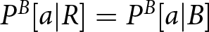 $P^B[a|R]=P^B[a|B]$.
Probability of accepting each color deal as a function of own attentional cost for a Level-1 player

2.4.3. Level-2
A Level-2 player best responds to the behavior of a Level-1 player. From the previous section, one can derive the SDSC of a Level-1 player as a function of their attention cost parameter. The main takeaway for a Level-2 player is that their SDSC will be a function of not only their own attention cost parameter but also the attention cost parameter of their opponent. That is, a Level-2 player is rationally inattentive, and realizes their opponent is also rationally inattentive.
Figure 3 illustrates the optimal SDSC as a function of one’s own attention cost parameter, holding the other fixed. One finding of interest is that dynamics concerning one’s own costs depend crucially on the cost of one’s opponent. Figure 3(a) shows a case in which the opponent has low costs of attention, while Figure 3(b) shows one in which they have high costs of attention.
If the opponent has low enough costs (underneath some threshold), then as their own costs increase, the probability of accepting favorable deals decreases. If the opponent has higher costs, however, then the probability of accepting unfavorable deals increases. The intuition is that a high-cost Level-1 opponent tends to accept most deals, making the ex-ante benefit from accepting high. A low-cost Level-1 opponent, however, tends to only accept their own favorable deals, making the ex-ante benefit from accepting low. Thus as own costs become sufficiently large, one who faces a low-cost opponent rejects all deals, while one who faces a high-cost opponent accepts all deals.
Probability of accepting each color deal as a function of own attentional cost for a Level-2 player, holding the attention cost of opponent constant at either a high or low level. (a) λ B low. (b) λ B high

Figure 4 holds fixed one’s own attention cost parameter, and varies that of the opponent. If an opponent has sufficiently low attention costs, a Level-2 player assumes they will do a very good job of discerning the state of the deal, and thus the benefits of paying costly attention are very low. Because of this, with low opponent costs, a Level-2 player will always reject. If the opponent has some sufficiently high costs, the Level-2 player assumes their opponent will accept all deals, and since the deals are ex-ante optimal, there will be a positive rate of acceptance for both favorable and unfavorable deals. Numerical analyses show a continuous mapping bridging these two extremes, with the probability of accepting a favorable deal strictly increasing with respect to opponent attention cost and, for the parameterizations relevant to the experimental design, the probability of accepting unfavorable deals also increasing in this cost.
Probability of accepting each color deal as a function of opponent attentional cost for a Level-2 player, holding fixed own attentional cost

3. Experimental design: Main treatment
The experiment is designed to test the ability of subjects to both anticipate and best respond to the information acquisition of opponents in the game examined theoretically. In anticipation of heterogeneity in subject behavior, I utilize a within-subject treatment that determines to what extent individuals best respond to the attention costs of themselves and of their opponents. The main experiment consists of four parts–three of them incentivized one of them a non-incentivized survey.
As the predictions in the theory section above rely on expected utility theory and assume I can observe the utilities of certain rewards, I use probability points as my incentivization scheme. That is, the earnings for an individual subject are points, valued from 0 to 100, which indicate their probability of winning a $10 bonus payment, in addition to a $10 completion payment. In my analysis, I can then normalize the utility of the $10 bonus payment to be 100, and the points will then directly correspond to their value in utility. To prevent hedging (especially concerning incentivized belief elicitation), only one randomly selected question from the incentivized portion of the experiment for payment is chosen.
The experiment itself took place online via Prolific and using oTree software (Chen et al., Reference Chen, Schonger and Wickens2016) software (Chen et al., Reference Chen, Schonger and Wickens2016). I will save the discussion on the decision to implement this as an online experiment versus an in-person experiment for after a description of the overall design.
3.1. Part one: Non-strategic decision task
The first part of the experiment serves two purposes: (1) introduce a real-effort attention task to the subjects, which will be used later in the strategic portion of the experiment, and (2) gauge individual level ability in this attention task. The attention task used in this experiment is the “dot task”, which has been established as a reliable task that rewards attentional effort with better outcomes, introduced by Dean and Neligh (Reference Dean and Neligh2023). The task consists of a square grid of red and blue dots. With 50% probability, there are more red dots than blue dots (a “red grid”), and with 50% probability, there are more blue dots than red dots (a “blue grid”). The task is then to determine whether the grid is red or blue. Subjects were given a maximum of 30 seconds to determine whether they think the grid is red or blue. A correct classification is rewarded 75 points, while an incorrect classification is awarded 25 points.
Because our theoretical predictions in the strategic setting rely on observing behavior in response to varying levels of attentional costs, I adapted the Dean and Neligh (2023) task to allow for variations in task difficulty. Thus, subjects are introduced to two difficulty levels in this part of the experiment—labeled “100-Dot” and “225-Dot”. As the names suggest, a 100-Dot grid is a 10-by-10 grid composed of 100 dots, and a 225-Dot grid is a 15-by-15 grid composed of 225 dots. Another difference between the two grid types is the difference in the number of dots between the “majority” and “minority” colors. On the 225-Dot grid, there are either 5 more blue dots (on a blue grid) or 5 more red dots (on a red grid). On the 100-Dot grid, there are 8 more blue dots or 8 more red dots. Piloting designed to elicit the difficulty of various dot tasks (only in decision-making settings) has determined that these two tasks are of consistently different difficulty levels, with the 100-Dot task being much easier than the 225-Dot task.Footnote 8 Figure 5 illustrates an example of these two grid types.
100-Dot grid (Left), 225-Dot grid (Right)

To elicit individual SDSC for each task, I utilize repetition. The two classification tasks are repeated 15 times each, for a total of 30 rounds. Because I am eliciting probabilities on the individual level, I did not want subjects to react to feedback, or demonstrate learning over time. Thus, no feedback about whether a subject was right or wrong on any particular round is provided until after the conclusion of the experiment. For ease of instruction, and to familiarize subjects with the structure of the strategic portion of the experiment, these 30 rounds are divided into 6 blocks of 5 rounds each. Within each block, the type of grid (100-Dot or 225-Dot) remains constant. Subjects are reminded of the upcoming grid type and the rules of the decision before each round, with an additional screen indicating any changes before each block.
3.2. Part two: Strategic game
Part two is the central part of the experiment. It consists of exactly the game described in Section 3. The values for vo, vH, and vL are set at 30 points, 90 points, and 10 points respectively. These values were chosen to give the data the “best chance” at observing differences in subject errors with respect to opponent task difficulty. First, note that the ex-ante optimality of accepting a deal is very salient. If both agents acquire no information at all and indiscriminately accept the deal, the expected payout is 50 points, versus 30 points for rejecting the deal.
At the start of this part of the experiment, subjects were assigned to one of two roles: Red player and Blue player. To avoid confusion and because the game is essentially symmetric, subjects were assigned to the same role throughout the experiment. Players were then told they would be randomly re-matched with a player of the other role type over 120 rounds. In each round, subjects played the game described in Section 3. Both players knew that a “Red Deal” and a “Blue Deal” were each equally likely. Their choice each round was to accept or reject the deal. A deal was “made” if both players accepted the deal. This would give 90 points to the player whose role color matched that of the deal and 10 points to the other player. If either or both players rejected the deal, they would each receive 30 points.
As in Part One of the experiment, subjects were again shown either 100-Dot or 225-Dot grids. The additional manipulation in this part of the experiment was to also vary their opponent’s grid type each round. Like in Part One, this was divided into 8 blocks of 15 questions each. Within each block, the grid type for the subject and their opponent remained constant. Crucially, subjects were repeatedly reminded of their grid type and their opponent’s grid type. Thus for each subject, I can elicit their SDSC in all four possible attentional setups. Again to avoid feedback and learning effects, no feedback was provided to subjects during this stage of the experiment. Thus, while the game was repeated 120 times, each round was treated as a one-shot game, where players were randomly rematched, and no feedback about previous games was given.
The 8 blocks of this stage of the experiment were divided into two each of the four possible task difficulty combinations (of own difficulty and opponent difficulty). Within-subject variation is especially important in testing the theoretical hypotheses of this strategic setup, as it allows us to estimate, for each subject, responsiveness to opponent task difficulty. As described in the preceding section, this will allow us to categorize subjects according to their level of strategic sophistication, something that between subject variation of own and opponent task difficulty would be ill-equipped to do.
Randomization occurred at the block level, where each of the four block types were presented in a random order. They then repeated this order twice for a total of 8 blocks. This structure was chosen to allow for randomization of the within-subject treatment variation, while also allowing me to elicit beliefs about opponent behavior after only the blocks in the second half of the experiment. This second benefit allows me to observe each within-subject variation twice, once before any beliefs are elicited, and once after such beliefs are elicited. In doing so, I am able to verify whether eliciting believes influences subject behavior, while maintaining randomization of the within-subject treatment. By asking beliefs only at the end of the experiment, I am only receiving beliefs that correspond to a more “experienced”, late-game subject. The concern that this may bias any conclusions about subject beliefs is mitigated by the lack of feedback. In addition, ex-post, the conclusion of the belief elicitation is a surprisingly incorrect distribution of subject beliefs, indicating that this design decision actually leads to, if anything, an underestimate of subject errors in beliefs.
Belief elicitation occurred at the end of blocks 5 through 8. At the beginning of Part 2, subjects were told there would be two additional questions at the end of these blocks but were not told they would be belief elicitation questions specifically. The goal of these questions is to elicit the subject’s beliefs of their opponent’s SDSC. To do so in a clear and understandable manner, subjects were asked to estimate the percentage of Red deals, and of Blue deals that their opponents accepted in the last block. Payment would then be made via a quadratic scoring rule,Footnote 9 where their payment would be the maximum of  $100-\frac{\text{Error}^2}{25}$ and 0 points, where the Error is the difference in percentage points between their belief and the actual probability of red or blue deals their opponents accepted in the previous block.
3.3. Part three: Other measurements
After the above rounds, a few potential co-variates are elicited. First, subjects play a variation of the 11-20 game proposed by Arad and Rubinstein Reference Arad and Rubinstein(2012). Subjects are randomly assigned into pairs and are each told to request a number of points between 51 and 60. Subjects receive the number of points they request, plus an additional 20 points if they request exactly one less point than their opponent. Arad and Rubinstein show that this is an easy-to-explain game that elicits the level of strategic sophistication of an individual. By measuring strategic sophistication through a separate game, I can verify that the subject pool is not unusually sophisticated or unsophisticated in comparison to what is usually found in the literature. It will also allow me to analyze behavior for subsets of the sample who score as more sophisticated in this measure.
Next, subjects are asked the three-question Cognitive Reflection Test (CRT) (Frederick, Reference Frederick2005) as another measurement of cognitive ability. Previous literature has often shown a correlation between this measurement and strategic sophistication, as well as performance in other economic games. This quiz was not incentivized, which is the standard approach in economic experiments involving the CRT. Again, this measure will allow me to assess the cognitive abilities of the subject pool and analyze behavior in the experiment for subsets who score higher on the instrument.
Finally, subjects filled out a brief survey. Aside from basic demographics (gender and education level), subjects were also asked to explain their strategy in part two of the experiment. This is done through a series of questions. First, subjects were asked to what extent they attempted to actually count the dots in each attentional setup of the game. They were then asked how their strategy depended on the task of their opponent for each of their own tasks. Finally, they were asked to give a free-form description of their overall strategy.
3.4. Online implementation of the experiment
The experiment was conducted online via Prolific, and I will argue that rational inattention experiments (in general), and more importantly strategic rational inattention experiments, are particularly well suited for such an environment. Firstly, an online environment allows subjects to go through the experiment at their own pace. In the above experiment, subjects could choose, for example, to inattentively click through each round of decision-making, and finish the experiment extremely early. Likewise, subjects could spend up to 30 seconds on each task, which could end up taking well over an hour. Allowing for both of these, and the spectrum in between, allows subjects to acquire information in a truly flexible and endogenous way—more in line with the spirit of rational inattention. An online environment allows for this kind of flexibility, whereas a traditional classroom lab experiment typically has a structure where participants can not leave the room until all subjects have completed the experiment. This can create unwanted social pressure effects (such as those to finish the experiment quicker than a subject would otherwise prefer) or cause subjects to spend more time than usual (since they would otherwise be sitting in a lab with nothing to do). Both of these issues are difficult to control for and could contaminate any treatment effects the researcher may be interested in.
The above underscores why this is an especially important problem for strategic information acquisition experiments. In most classroom labs, it becomes very obvious the average response time of decisions of the other subjects in the lab (via sounds of clicking mice and keyboards or seeing other subjects sitting idly). This has the potential to create large session-level effects and introduces a noisy signal of opponent strategy that is difficult to model or control for.
In an online environment, subjects can play the game at their own pace. Subjects proceed through all stages without waiting for any other player’s actions. Because no feedback is provided, this is feasible in the design outlined above. Subjects are told that payments will be calculated once all subjects in the session have completed the experiment, no later than 7 days after that subject has finished. At this time, subjects are given a Qualtrics survey link where they log in with their Prolific credentials and are shown their award in points. These points then translate to their probability in percent of winning a $10 bonus payment. I utilize the lottery mechanism designed by Caplin et al. Reference Caplin, Csaba and Leahy(2020) to credibly award the bonus with the correct probability. Subjects are shown a timer synced to their computer system clock in milliseconds. They can stop this clock once and only once, and the milliseconds in one’s and ten’s constitute a random number, where a number less than their point value results in the bonus payment. Subjects have access to a practice version of this task before taking part in the experiment, to credibly signal the randomness of the device.
4. Results: Main treatment
Sessions for the experiment took place in July and August of 2022. In total, 100 subjects completed the experiment online. Subjects were recruited and paid via Prolific and participated in the experiment via oTree on their computer browserFootnote 10 Demographically, all subjects were residents of the United States, had at least a high school education, were fluent in English, and were between the ages of 18 and 30. Subjects were also restricted from taking the experiment multiple times, and the subject pool was balanced across sex.Footnote 11 The median duration of the experiment was 42.5 minutes, and the mean duration was 50.0 minutes. Average earnings were $15.50, including the $10 participation fee.
4.1. Decision task: Difficulty validation
The first priority is to verify that the two tasks were of consistently different difficulty levels. To do this, I examine the accuracy rate of classification during the decision-making rounds. Recall that each participant played 15 rounds of each task type. Figure 6 shows the average accuracy across the two tasks and the average difference between the two, with error bars to indicate one standard error. In the 225-Dot task 61% of grids were correctly classified, while in the 100-Dot task this proportion was 84%.
Average accuracy by task (standard errors clustered by subject) and the average difference in Part 1 of the experiment (decision-making task)

Table A1 in Appendix A presents results from a logistic regression and a linear probability model of correctness on round, true color, and task difficulty, with errors clustered at the individual level. Regression analysis confirms that the 225-Dot task is significantly more difficult than the 100-Dot task. In addition, there are no aggregate round effects, nor any systematic differences in discerning red or blue images.
It is also of interest to examine any heterogeneity in ability across the two tasks. There is indeed substantial heterogeneity in ability.Footnote 12 Figure 7 plots the probability of correct classification in the 100-Dot task on the vertical axis and the probability of correct classification in the 225-Dot task on the horizontal axis, with each point representing an individual subject, along with the 45-degree line.
Individual heterogeneity in decision task accuracy

While there is substantial heterogeneity in accuracy across individuals, the vast majority of subjects are more accurate in the 100-Dot task than in the 225-Dot task. This is evident by the majority of points in Figure 6 lying above the 45-degree line. Just 12 of the 100 subjects did not have higher accuracy in the 100-Dot case (including 4 subjects who had the exact same accuracy in the two tasks). These findings are indicative that the tasks developed are almost universally ordered in terms of difficulty.
In addition, the probability of correct classification in the two tasks is ideally calibrated for this setting. The 225-Dot task is very difficult; however, the average accuracy is 61% which is above what one could get by randomly guessing (i.e. the task is difficult but not impossibly so). The 100-Dot task, on the other hand, has a significantly higher accuracy rate of 84%, which is significantly lower than perfect accuracy (i.e. the task is easy but not trivially so).
4.2. Strategic behavior
Having validated the manipulation in task difficulty, I now turn to the subjects’ behavior in Part 2 of the experiment. For all results, a state will be referred to as “favorable” if the color of the deal matches the color of the role, with a state being “unfavorable” otherwise.
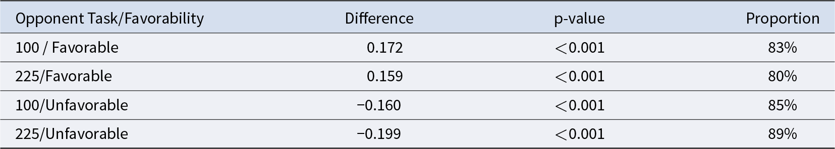
A basic first test that subjects understand the strategic setting is to verify that  $P[a|\text{Favorable}]\geq P[a|\text{Unfavorable}]$. Table 1, Column 2 shows the mean difference in acceptance probability between favorable and unfavorable deals for that attentional setup. Column 3 reports p-values from a two-tailed, paired t-test between the probability of accepting a favorable and unfavorable deal for each setup. Column 4 reports the percentage of subjects who accept weakly more favorable deals than unfavorable deals for each setup, while Column 5 reports the percentage of subjects who accept strictly more favorable deals than unfavorable deals.
Attention checks for strategic rounds, columns 4 and 5 report proportion of subjects with weakly and strictly positive differences between accepting favorable and unfavorable deals

Average differences are highly significant and are non-negative for a large majority of the subjects. Note that 20% of subjects have strictly negative differences in the 225/225 setup. This is largely an artifact of a higher proportion of subjects inattentively guessing in the more difficult settings. Nevertheless, 80% compliance in the worst-case scenario is more than sufficient in such an experiment.
I will next examine the SDSC of subjects across attentional setups. Figure 8 visualizes the average data of all 100 subjects, with standard errors clustered at the level of the subject and difficulty level.Footnote 13
Probability of accepting favorable and unfavorable deals by setup

There is a significant effect of own-task difficulty on accepting both favorable and unfavorable deals. Table 2 shows the difference in acceptance probability, holding fixed the opponent difficulty and favorability of the deal. Column 2 shows the difference of  $P[a|\text{Own 100-Dot}]-P[a|\text{Own 225-Dot}]$, Column 3 shows the p-value of the corresponding paired t-test, and Column 4 shows the percentage of subjects whose individual effect is in the same direction as the group effect. The findings demonstrate that, almost universally, subjects who face the more difficult task accept far fewer favorable deals, and far more unfavorable deals. The average difference between accepting favorable deals and accepting unfavorable deals is roughly 15.2% for those with 225-Dot tasks, while this number is 49.8% for those with 100-Dot tasks.
Differences in probability of accepting a deal when given a 100-Dot task and a 225-Dot task, holding favorability of deal and opponent task fixed, with column 4 indicating the proportion of subjects with the same sign as the aggregate
Despite the above facts, Figure 8 also shows that there is no aggregate effect of opponent difficulty on subject SDSC. There is no significant treatment effect of the opponent’s task on the probability of accepting in either a favorable or unfavorable state. Recall from the theory section that insensitivity of behavior to the opponent’s task is a defining feature of “Level-1” strategic behavior. Subjects who have a higher level of sophistication should decrease their probability of accepting both favorable and unfavorable deals in light of an easier opponent task. This is because opponents facing an easier task (1) accept more deals that would be favorable to the subject (and thus unfavorable to the opponent) and (2) reject more deals that would be unfavorable to the opponent (and thus favorable to the subject). This causes the expected value of accepting a favorable or unfavorable deal to decrease, which the theory then claims should lead to a decrease in the probability of accepting either type of deal.
Mirroring Table 2, Table 3 shows the difference in acceptance probability, holding fixed own difficulty and deal favorability. Column 3 shows the p-value of the corresponding paired t-test, while Columns 4-6 show the percentage of subjects where the difference (225-Dot opponent minus 100-Dot opponent) is positive, equal, and negative, respectively.
Differences in probability of accepting a deal when facing 225-Dot opponent and 100-Dot opponent, holding favorability of deal and own task fixed, with columns 4-6 indicating the proportion of subjects with a difference of each sign

These findings again suggest that there is no aggregate effect of the opponent’s taskon SDSC. Individual behavior appears to be approximately symmetric around this mean 0 difference, suggesting that deviations from this aggregate value are more likely to be noise than systematic heterogeneity.
To confirm this more rigorously, I run both logisticFootnote 14 and linear regressions of:
 \begin{equation*}
y_{it} = \beta_0 + \beta_1 \text{Own100}_{it} + \beta_2 \text{Opponent100}_{it} + \beta_3 \text{Own100}_{it} \ast \text{Opponent100}_{it} + \beta_4 t + \epsilon_{it}
\end{equation*}
\begin{equation*}
y_{it} = \beta_0 + \beta_1 \text{Own100}_{it} + \beta_2 \text{Opponent100}_{it} + \beta_3 \text{Own100}_{it} \ast \text{Opponent100}_{it} + \beta_4 t + \epsilon_{it}
\end{equation*}where yit is an indicator for when subject i accepts a deal in round t. The regression is run twice—once for when the deal is favorable, and once for when it is unfavorable. I do this because the coefficients on the independent variable are likely to be different in each case. “Own100” is an indicator for when a subject faces a 100-Dot task in a given round and “Opponent100” is an indicator for when a subject’s opponent faces a 100-Dot task in a given round. In addition, errors are clustered on the subject and own task difficulty levels. The results for these regressions are presented in Table A2 in Appendix A.
First, note that own task difficulty is highly significant for either acceptance probability. The effect of Own100 is large and positive for the favorable case (i.e. people correctly accept more favorable deals), and large and negative for the unfavorable case (i.e. people correctly reject more unfavorable deals). The opponent task is only significant (p < 0.10) in the unfavorable case, suggesting subjects make slightly fewer (roughly  $3\%$) mistakes in accepting unfavorable deals when their opponent has an easy task. However, the opponent’s task is not at all significant for the favorable case, and the interaction terms are not significant in either case. Finally, another worry with any experimental study involving many repeated tasks is that performance will change over time due to fatigue or learning. This is especially crucial to check in this setting, as my analysis implicitly assumes that behavior in each game is independent of the other games (this assumption allows one to treat an individual’s probabilities of accepting deals in various states as true SDSC in the rational inattention sense). The coefficients on Round support this assumption, which is also supported by previous experimental tests of rational inattention (Dean & Neligh, Reference Dean and Neligh2023).
4.2.1. Cluster analysis to determine distribution of strategic levels
While Table 3 provides suggestive evidence that the aggregate results from the logistic regression are unlikely to be masking meaningful individual-level heterogeneity, I now provide more exhaustive support for this claim. I achieve this by running regressions on each individual’s behavior on indicators for the attentional-setup of the round. The coefficients of this regression will reveal to what degree each subject is reacting to their own task difficulty as well as that of their opponent. I then run cluster analysis on these coefficients to categorize subjects based on their reactivity to opponent difficult levels, the results of which naturally coincide with the level-k predictions derived in Section 2.
Specifically, for each subject i I run the linear probability model of
 \begin{equation*}
y_{it}=\beta^i_0 + \beta^i_1\text{Own100}_{it} + \beta^i_2\text{Opponent100}_{it}+\beta^i_3\text{Own100}_{it} \ast \text{Opponent100}_{it}+\epsilon_{it}
\end{equation*}
\begin{equation*}
y_{it}=\beta^i_0 + \beta^i_1\text{Own100}_{it} + \beta^i_2\text{Opponent100}_{it}+\beta^i_3\text{Own100}_{it} \ast \text{Opponent100}_{it}+\epsilon_{it}
\end{equation*}for favorable states and for unfavorable states, where once again yit is a dummy indicator for accepting the deal. Note that by excluding the round variable, the above linear probability regression gives the true marginal probabilities of each of the independent variable dummies. Given the lack of a time trend in the aggregate data, this choice is without much loss.
This results in a collection of β i coefficient estimates for each individual. Because this is a linear probability model and not a logistic model, these coefficients are directly comparable across individuals. My primary interest lies in the heterogeneity of coefficients on the opponent task’s, and the interaction between the opponent’s and own task. Thus I create a new set of four coefficient estimates for each individual (opponent and interaction coefficients for favorable and unfavorable regressions).
On this new data set of coefficients, I run the mixture models cluster analysis used by Brocas et al. Reference Brocas, Carrillo and Wang(2014) via the mclust package in R (Fraley & Raftery, Reference Fraley and Raftery2007). This analysis assesses any possible heterogeneity by calculating possible clusters of up to 9 groups using 14 possible models and then choosing the combination with the highest Bayes Information Criterion (BIC). The benefit of this approach is that it assesses any possible heterogeneity without assuming the exact nature of this heterogeneity, or the number of possible clusters.
The results of this clustering analysis support the hypothesis that there is very little meaningful heterogeneity in the subjects’ sensitivity to their opponent’s task. Figure A1 in Appendix A shows the BIC value for each model and each number of clusters (up to 9). The winning model is that in which the clusters have ellipsoidal shape, equal volume, and equal orientation (EVE) and with 2 clusters. These two clusters consist of 95 subjects and 5 subjects. Table 4 reports the average coefficient values for each cluster. The cluster which represents the behavior of 95 of the 100 subjects strongly resembles that of a level-0 or level-1 player, given that all coefficients corresponding to opponent interaction are extremely close to 0. The remaining 5 subjects show behavior mostly in line with level-2 predictions, choosing to accept both favorable and unfavorable deals less often when opponents have a low cost of attention. We note that, compared to previous studies on level-K reasoning, our findings are an unusually high number of subjects with less than two levels of strategic sophistication.
Mean parameter values for optimal clusters

Figure A2 in Appendix A shows the scatter plots associated with this classification. The classification again confirms that by and large that the aggregate effects are not hiding meaningful heterogeneity. 95% of subjects fall into a cluster in which the average percentage effect of the opponent having an easy task is between 0% and 2%. Five subjects can be categorized into a cluster where these differences are much larger, indicating an average percentage effect of up to 39%. This suggests that while some subjects appear to have higher levels of strategic sophistication, the vast majority of participants behave extremely similarly to Level-1 types–with behavior invariant to the attentional costs of their opponents. This proportion of Level-1 types is far greater than commonly found in other economic games—an exhaustive study by Georganas et al. Reference Georganas, Healy and Weber(2015) finds between 28% and 71% proportion of Level-1 players, depending on the game.
4.3. Beliefs
The preceding section demonstrated a strong effect of own task on behavior, and essentially no effect of the opponent’s task on behavior. While this offers strong evidence of an out-sized lack of strategic sophistication, it is yet unclear what mechanism is underlying this behavior. There are two clear possibilities: subjects have difficulties in anticipating opponent behavior (i.e. their beliefs are incorrect), or the subjects’ information acquisition is not sensitive to incentives (i.e. the subjects are not rationally inattentive and ace fixed abilities to discern the two states in each task). The following two sections, alongside a follow-up experiment described thereafter, provide support for the first of these two hypotheses. The current section shows that beliefs are largely incorrect and noisy. The following section shows that subjects largely seem to adjust their attention in response to what they perceive to be the incentives of doing so, which are themselves functions of these incorrect beliefs.
As a reminder, all subjects are asked to report their beliefs about how frequently their opponents accepted deals of either color in the preceding block (i.e. under the preceding block’s attentional setup). That is, I elicit, in an incentive-compatible manner, their beliefs about the SDSC of their opponents. Figure 9 shows the analogous plot of Figure 8, however, this time showing the subjects’ mean beliefs of their opponents accepting in the various attentional setups. Note that the figure takes the opponent’s perspective in labeling a state as “favorable” or “unfavorable” (so that the figure is exactly comparable to that of Figure 8).
Beliefs of opponent behavior by setup

One minimal check to ensure people understood the strategic setup of the game is to see whether they expected their opponents to accept more often in their opponent’s favored state. The findings confirm this on the aggregate. Paired t-tests show that subjects believe opponents have a 15.8 and 15.3 percentage point higher acceptance rate in favorable deals over unfavorable deals when the opponent has a 225-Dot task and the subject has a 225-Dot and 100-Dot task, respectively (p < 0.001 for both tests). When the opponent has a 100-Dot task, these numbers are 25.6% and 26.2% (again with p < 0.001 for each test).
Comparing the above numbers to the actual SDSC of the subjects, however, reveals that subjects hold largely incorrect beliefs about opponent behavior and information acquisition. Table 5 is analogous to Table 1, however, it now shows the differences between reported beliefs that an opponent accepted their favorable deal versus their unfavorable deal. Note that Table 1 shows that the average difference in accepting favorable and unfavorable deals is nearly 50% for subjects, while the analogous difference in beliefs is only 26%. The gap between differences in Table 1 for the 100-Dot task and the 225-Dot task is approximately 35%, while this gap is only 10% for beliefs. However, Table 5 also shows that people clearly understood the basic strategic setup—columns (4) and (5) show that a vast majority of subjects understood their opponent would be selecting more deals of the subject’s unfavorable color than that of the subject’s favorable color. However, a very high percentage of subjects, believe these two probabilities to be equal, as demonstrated by the large differences between columns (4) and (5).
Differences between reported beliefs that opponent accepted their favorable versus unfavorable deal, columns 4 and 5 report proportion of subjects with weakly and strictly positive differences in beliefs

To further examine these findings, Figure 10 displays histograms for the differences in Favorable/Unfavorable acceptance beliefs under each attentional setup. This figure, along with Table 5, indicates that a large number of subjects with what are essentially Level-1 beliefs—i.e. they roughly believe  $P[a|R]=P[a|B]$. While very few subjects report an incorrect sign (negative) for this statistic, the main takeaway of the figure is the sharp concentration of subjects with reported beliefs of opponent favorable and unfavorable acceptance probabilities which are extremely close to one another.
Histogram of difference in favorable and unfavorable accept belief, by attentional setup

The above could represent two possible mechanisms. Subjects either truly believe their opponents are acquiring very little information, or they have a large degree of cognitive uncertainty about their opponent’s information acquisition, and so for all intents and purposes, they behave as if their opponent is acquiring very little information. While the present experiment cannot distinguish these two specific mechanisms, I believe the second to be more plausible. Given that subjects themselves acquire significant information throughout the experiment, as demonstrated throughout Section 3.2, it seems likely that they believe their opponents are acquiring information as well. Subjects were also fully aware of the strategic setup of their game, as they were forced to answer all comprehension questions successfully to begin the experiment.Footnote 15
Finally, Figure 9 also clearly shows that there is no significant effect of own task on beliefs about opponent behavior. This suggests that the players’ beliefs are consistent with no larger than two levels of strategic sophistication, and also indicates that the discrepancies found are an effect of their opponents’ task only, and not a reflection of the subjects’ own immediate experience.
4.4. Beliefs as the mechanism for strategic unsophistication
Whatever the mechanism behind subjects’ largely incorrect beliefs about opponent SDSC, it is clear that even under incentivization they are largely unable to correctly anticipate opponent behavior. The next step is to see whether the subjects themselves acquired information as if their opponents were playing according to these incorrect beliefs.
To do this, I run the same linear regression as presented in Table A2 of Appendix A but instead substitute two belief variables—“BA” and “BD”—along with their interaction terms with the dummy indicating a 100-Dot task for the subject, in place of dummies for the opponent task. Here, “BA” refers to the unconditional belief that their opponent chose to accept, calculated by taking the average of the two belief elicitations for that round’s attentional setup. “BD” refers to the difference in beliefs of the opponent accepting deals in their favorable state and their unfavorable state for the relevant attentional setup, i.e. the values illustrated in Figure 9. These two transformations of the subjects’ elicited beliefs were chosen instead of the two raw beliefs because of the high correlation between a high belief of acceptance of a favorable deal with that of an unfavorable deal. Thus coefficients on either of these values alone are difficult to interpret independently of the other coefficient. The interpretation of the coefficient on “BA” then is how sensitive a subject’s behavior is to the unconditional likelihood of their opponent accepting, while the coefficient of “BD” is the causal impact of one’s beliefs about the extent of their opponent’s information acquisition on their behavior. The dummy for the opponent task was excluded from these regressions as it is highly correlated with beliefs (as seen in Table 5), leading to multicollinearity concerns. Once again, I run this regression twice, for favorable and unfavorable deals, and errors are clustered on the combination of own task difficulty and subject. The coefficients on the relevant interaction terms then indicate how these effects change when the subject is shown a 100-Dot task.
Table 6 presents the results of this regression, while table A3 in Appendix A shows the analogous logistic regression. Columns (1) and (3) regress on the entire sample, while Columns (2) and (4) regress on only the subset with non-negative values for all four “BD” measurements (76 out of 100 subjects).
Linear probability regression of accept, by favorability

* Note: p < 0.1; ** p < 0.05; *** p < 0.01.
In summation, the above analysis suggests that (1) subjects’ reported beliefs have significant predictive power on their choice behavior, and (2) the signs on these reported beliefs mostly align with what rational inattention theory predicts. However, due to the caveats explained above, caution must be used when interpreting these results with respect to the reliability of elicited beliefs and whether these beliefs are merely a reflection of own behavior. For these reasons, I conduct a follow-up treatment, to be described in Section 5.
5. Discussion and experiment two
5.1. Discussion of main experiment results
The main conclusion from the preceding experiment is an out-sized lack of strategic sophistication in this extremely simple economic game environment. Recall from the theoretical discussion that when facing an opponent with low attention costs (or one who has an easier task), the benefits of discerning a good and a bad deal decrease. This is because accepting a favorable deal is likely to yield little in the way of positive utility (since the opponent is likely to reject it), and accepting an unfavorable deal is likely to be quite costly (since the opponent is like to accept it). These features make accepting the deal much less attractive when compared to the safe outside option acquired by rejecting it. Subjects do not respond in this way, even though they themselves perform much differently when facing the two tasks. Furthermore, as shown in Appendix B.1, they spend the same amount of time deciding on whether or not to accept a deal regardless of the task of their opponent, again suggesting that players are not adjusting their attention strategy in a way a strategic agent should. The results are likewise robust when looking at subjects’ reported strategies as given in the survey, as described in Appendix B.2.1. Appendix B.2.2 shows that the experimental sample is strategically sophisticated in the cognitive reflection test and the 11-20 game, ruling out the possibility of a simply low-sophistication sample.
Belief elicitations and regressions of behavior on these beliefs suggest the mechanism behind the low levels of strategic sophistication to be inaccurate and perhaps uncertain beliefs. In each of the four attentional setups, the plurality of subjects report beliefs that the probabilities an opponent accepts a favorable and an unfavorable deal are essentially the same. These correspond to the beliefs held by “Level-1” agents in the theoretical framework. Whether through simply incorrect beliefs or through cognitive difficulty in anticipating opponent behavior, these mistaken beliefs seem to drive the “Level-1” behavior of agents. Specifically, regression analysis suggests that attention does seem to respond to beliefs, and that these beliefs are simply wrong. To test this hypothesis, I conducted a follow-up experiment in which I removed the uncertainty about opponent behavior entirely. By keeping all else equal, including the incentives at play in the experiment, I can also verify that the lack of response to opponent difficulty is not simply an artifact of low experimental incentives (a $10 payment for 1 of 159 rounds).
5.2. Experimental design: Experiment two
To further test whether the mechanism behind the results of the previous experiment was indeed cognitive limitations of strategic thinking and forming correct beliefs, I conducted a follow-up experiment. This follow-up experiment followed the exact design of the main experiment, however instead of playing other subjects, subjects played against computer players who followed a pre-specified strategy.
Specifically, instead of being matched with either “225-Dot” or “100-Dot” human subjects, subjects are now matched with either “30:80 Computer” or “50:65 Computer”. A 30:80 Computer accepts a deal of the subject’s color 30% of the time, and a deal of the opposing color 80% of the time, with the 50:65 Computer being analogous. These numbers were specifically chosen to mirror the average behavior seen by participants in the main experiment. The subjects were told the meaning behind these labels on multiple occasions during the instructions and constantly reminded throughout the experiment. In addition, subjects were quizzed for their comprehension of the computer behavior and had to correctly answer the quiz to proceed with Part 2 of the experiment.
Just as in the main experiment, subjects played 120 rounds of these games, spread across 8 equally sized blocks. There were 2 blocks for each combination of own-grid task and opponent Computer type. Crucially, this is all entirely identical to the main experiment, with the only difference being the removal of all uncertainty about their opponent’s strategy. For the belief elicitation questions that appear at the end of blocks five through eight, the subjects were asked to report their beliefs about how often a randomly selected subject of the other role type behaved when they faced the same block setup (own task and computer opponent) as the subject did.
5.3. Results: Experiment two
The experiment took place again virtually via Prolific, with subjects filtered to be American residents between the ages of 18 and 30 with at least a high school education, and again the subject pool was balanced across sex. Importantly, any subjects who may have taken part in Experiment 1 were excluded. Experiment Two was conducted on 40 subjects in September 2022.
First, I recreate the main analyses from the main experiment in the new treatment. Now, instead of referring to opponent tasks, I instead refer to computer players. Recall playing a “30:80” computer is equivalent in behavior to playing the average 100-Dot opponent, while a “50:65” computer is equivalent in behavior to playing the average 225-Dot opponent. Figure 11 shows the probability of accepting a deal in favorable and unfavorable states, for each attentional setup. Contrary to the main experiment, there is a strong significant effect of computers opponent on subjects’ SDSC. When subjects face a 30:80 computer (the payoff equivalent of facing a 100-Dot opponent in the main experiment), they rationally shade their SDSC towards rejection–favoring the reduction of accepting unfavorable deals over the reduction of rejecting favorable deals. When subjects face a 50:65 opponent, they prioritize reducing errors in rejecting favorable deals over reducing errors in accepting unfavorable deals. This strong and significant effect of computer opponent on SDSC also confirms that SDSC does indeed vary with incentives and that the lack of reactivity in the main experiment was not due to insufficiently large stakes.
Probability of accepting favorable and unfavorable deal by setup, computer treatment

Table 7 shows the average differences in accept probability when the own task is 100-Dot vs 225-Dot, holding computer opponent and favorability of the deal fixed. Note that Column 2 shows the average difference, Column 3 shows the p-value from the associated paired t-test, and Column 4 shows the percentage of subjects whose data has the same sign as the average. Once again the vast majority of subjects make fewer errors when given a 100-Dot task.
Differences in probability of accepting a deal when given a 100-Dot task and a 225-Dot task, holding favorability of deal and computer opponent fixed, with column 4 indicating the proportion of subjects with the same sign as the aggregate

Table 8, however, shows the average differences in accept probability when the computer is 50:65 versus 30:80, holding the subjects’ task difficulty and favorability fixed. Note that Column 2 shows the average difference, Column 3 shows the associate p-value, and Columns 4-6 show the percentage of subjects whose difference is positive, equal, and negative.
Differences in probability of accepting a deal when facing 50:65 computer and 30:80 computer, holding favorability of deal and own task fixed, with columns 4-6 indicating the proportion of subjects with a difference of each sign

In sharp contrast to the analogous Table 3, there is a strong positive effect of a 50:65 computer on the probability of accepting a deal for all cases except for when subjects have a 100-Dot task and face an unfavorable deal (although at 40 subjects, this experiment does have lower power than the main experiment). While Table 4 showed roughly equal amounts of subjects had a positive and negative sign for this difference, now in all four cases significantly more subjects had a positive sign than a negative sign. This again supports the argument that subjects were largely sensitive to computer opponent accuracy in a way that they were not towards human opponent accuracy.
Finally, regression analysis can verify the above results, and findings are reported in Table A4 in Appendix A. Unlike in the main experiment in which there was little if any effect of the opponent’s task on accept probability, there is a strong negative effect of a 30:80 computer on accept probability in either favorability condition. Again this supports the story of the subjects favoring the reduction of erroneously accepting unfavorable deals when facing a more accurate computer opponent.
Following the analysis of response times in the main experiment which showed no aggregate response toward the opponent’s task, I run analogous regressions on this treatment. The results of this regression appear in Table A5 of Appendix A. The effect of having a 100-Dot task opponent equivalent has a negative, significant (p < 0.10) effect on response times in the own 225-Dot treatment, and a negative but non-significant effect in the own 100-dot treatment. When the computer is separating very well, subjects on average spend less time gathering information, and simply reject the deal more often. This is indicative of a rational allocation of mental resources, as the possible benefits of spending longer on the task grow smaller in this case relative to the constant outside option that requires no mental effort. Also of note, the average response times are significantly longer in this treatment than in the main treatment. One possible explanation is that the reduced uncertainty about opponent behavior translated to more explicit incentives for information acquisition and thus more baseline mental effort devoted to doing so.
6. Conclusion
In the simplest possible strategic setting where multiple agents face costs of information, I have found that subjects play in a strategically unsophisticated manner. They acquire information about the state of the world, but they do not acquire this information as if they are playing a strategic opponent. Through careful analysis of subjects’ elicited beliefs, I find that the mechanism through which this behavior occurs is beliefs—subjects simply do not anticipate the information acquisition of their opponents. In the follow-up experiment, I eliminate the possibility of this mechanism by having subjects play against automated computers with a transparent strategy. Contrary to the results of the main experiment, here subjects significantly adjust their information acquisition strategies in the direction that the theory predicts.
One explanation for why strategic sophistication may be even lower in games with information acquisition than in standard settings may be “cognitive uncertainty”. The cognitive uncertainty literature, beginning with Enke and Graeber Reference Enke and Graeber(2019) suggests that when people are cognitively uncertain, their “decisions are severely attenuated functions of objective problem parameters”. In the present setting, this could mean that the cognitively complex task of anticipating opponent information acquisition causes people to systematically act as if playing a “Level-0” opponent (one with no information acquisition at all). The high degree of “Level-1” beliefs and the generally high variation in reported beliefs is suggestive of this explanation.
Yet another explanation lies within the work on costly depth of reasoning by Akerlof Reference Akerlof(1970). Again coinciding with the above phenomenon, anticipating opponent information–and thus behavior may be prohibitively costly given the incentives for doing so. Thus while information acquisition responds sharply to the subjects’ own task (in experiments 1 and 2), and incentives (in experiment 2), it does not respond to the opponent’s task. Attention is costly in this setting, but not prohibitively so. This simply may not be the case with the costs inherent in strategic reasoning.
Both of the above explanations also deliver insights into why the results of the present paper differ qualitatively from those found in Almog and Martin Reference Almog and Martin(2024). In their paper, the authors find that inattentive buyers adjust their information acquisition strategies in response to changes in the strategic incentives of fully-informed sellers. An inattentive buyer in their setting only has to perform standard strategic reasoning, not unlike that present in standard strategic communication games, in order to understand the incentives of information acquisition. In this paper’s setting, inattentive players are forced to understand the cognitive constraints of their opponents in order to understand the incentives of information acquisition. Thus the difference in the two paper’s results is likely a result of the difficulty of understanding opponent’s cognitive constraints or, in other words, the difficulty of possessing an accurate theory-of-mind (an idea from psychology brought to economics by Ohtsubo & Rapoport Reference Ohtsubo and Rapoport(2006). This difficulty can also be modeled by a costly depth of reasoning, as in the endogenous depth of reasoning literature introduced by Alaoui and Penta Reference Alaoui and Penta(2016). This work has shown that levels of strategic reasoning are perhaps best thought of as not fixed, personal levels, but as reactions to the costs and benefits of strategic reasoning. The results of this experiment strongly suggest that costs of strategic reasoning are especially high in settings in which, to predict the actions of an opponent one must be able to predict that opponent’s information acquisition. These higher costs lead to an extremely high observed proportion of “level-1” players, as compared to other strategic settings. Perhaps the most important future direction for this research is to further study the interaction between costs of information and costs of strategic reasoning, and how the two may amplify each other, as observed in this experiment.
Supplementary material
The supplementary material for this article can be found at https://doi.org/10.1017/eec.2025.8.
Availability of data and materials
All data and materials are available in their original formats at https://doi.org/10.17605/OSF.IO/W2EQZ.
Acknowledgements
This research has been generously supported by the Center for Experimental Social Science at New York University. I am grateful to Andrew Caplin, David Cesarini, Guillaume Frechette, and Andrew Schotter for their guidance and support. I also thank David Almog, Srijita Ghosh, Eungik Lee, Daniel Martin, Minu Philip, Anwar Ruff, Isabelle Salcher, Matheus Silva, seminar participants at the 2022 ESA Eurpoean and North American Meetings, and two anonymous referees for their comments and suggestions.
Replication packages
To obtain replication material for this article, https://doi.org/10.17605/OSF.IO/W2EQZ.
Code availability
All corresponding code is available at https://doi.org/10.17605/OSF.IO/W2EQZ.
Authors’ contributions
Not applicable.
Conflict of interest/Competing interests
The author has no relevant financial or non-financial interests to disclose.
Disclosure Statement
The views expressed in this paper are my own and not necessarily those of the Federal Trade Commission or of any individual Commissioner.
Funding
Funding for the experiments present in this paper was provided by the Center for Experimental Social Sciences at New York University through Professor David Cesarini.
Ethics approval
The research present in this experiment was approved by the New York University IRB, protocol number IRB-FY2022-6222.
Consent to participate
Consent for participation in the studies included in this paper was obtained in accordance with the IRB approval mentioned above.
Consent for publication
Not applicable.

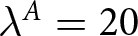

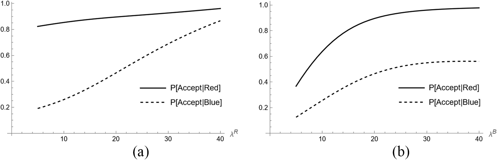
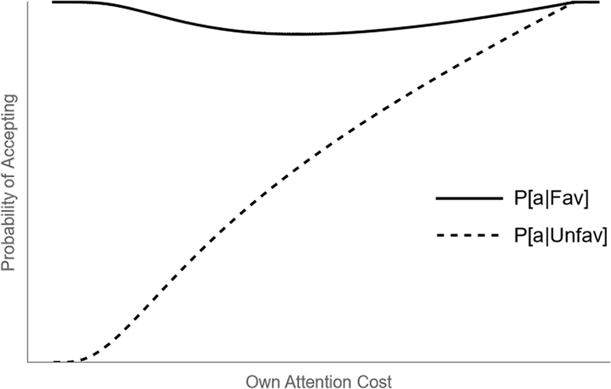
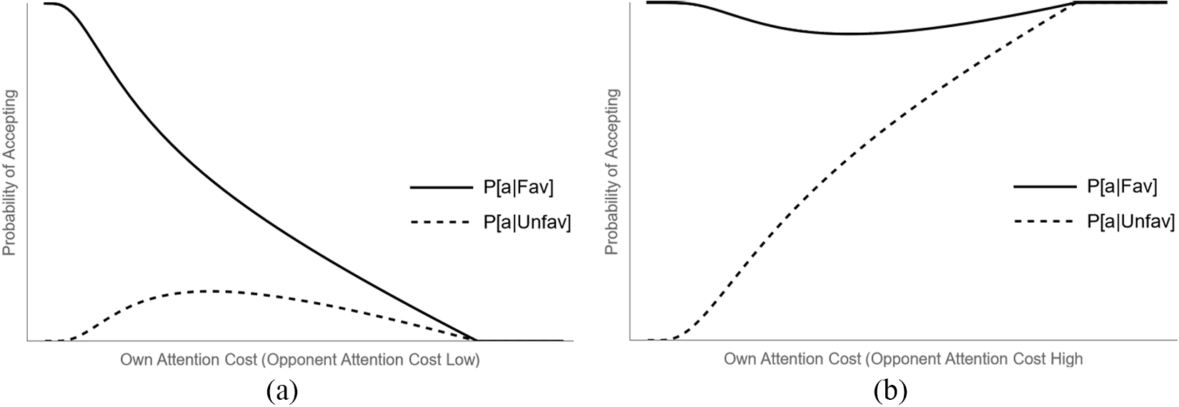
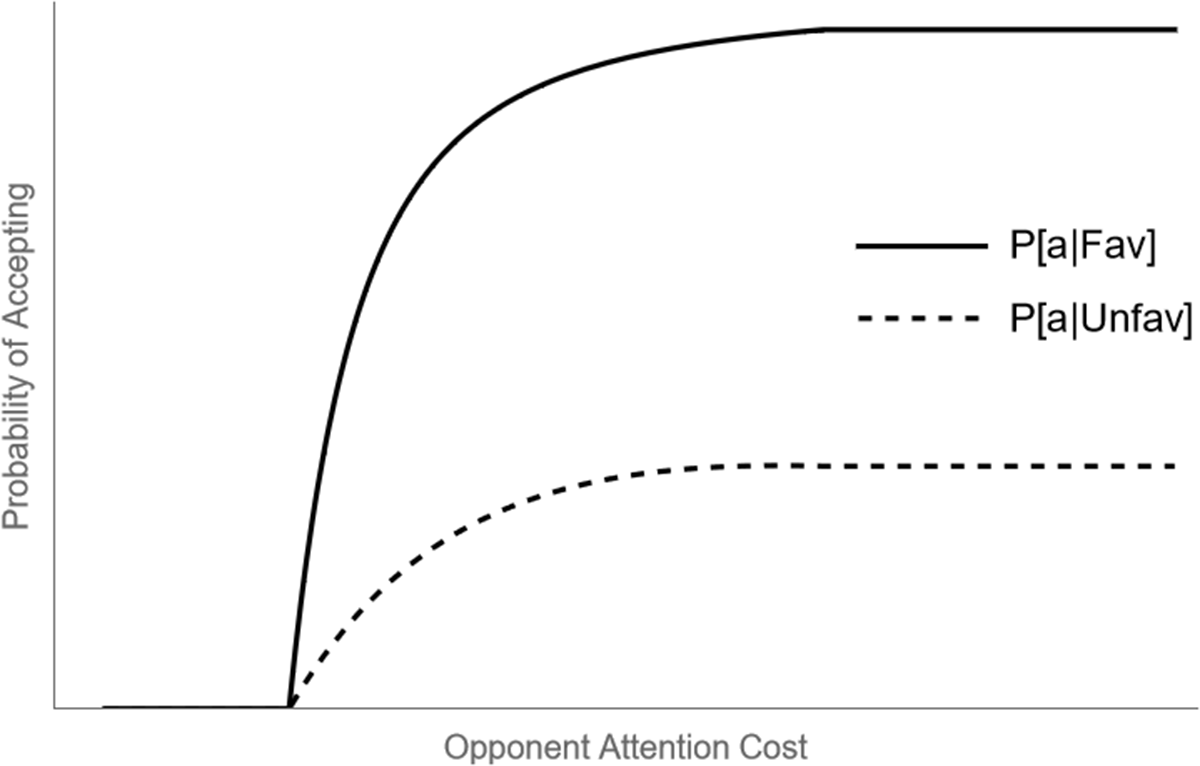
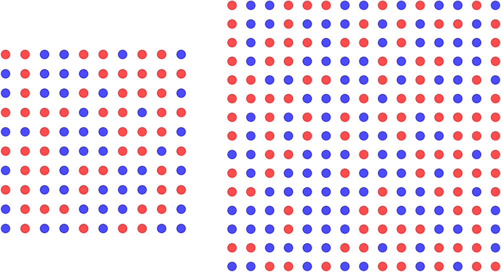
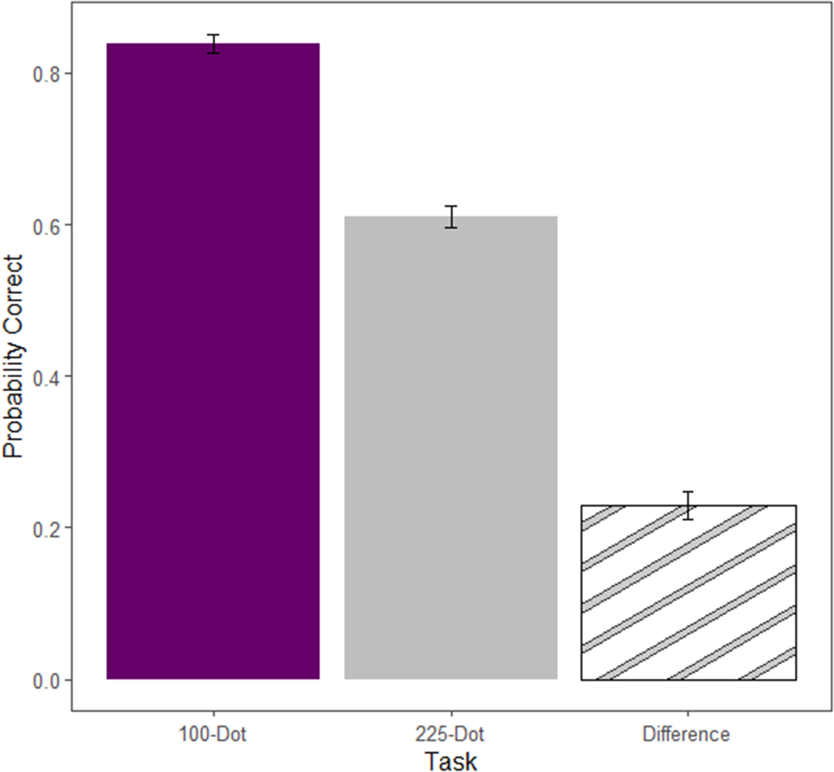
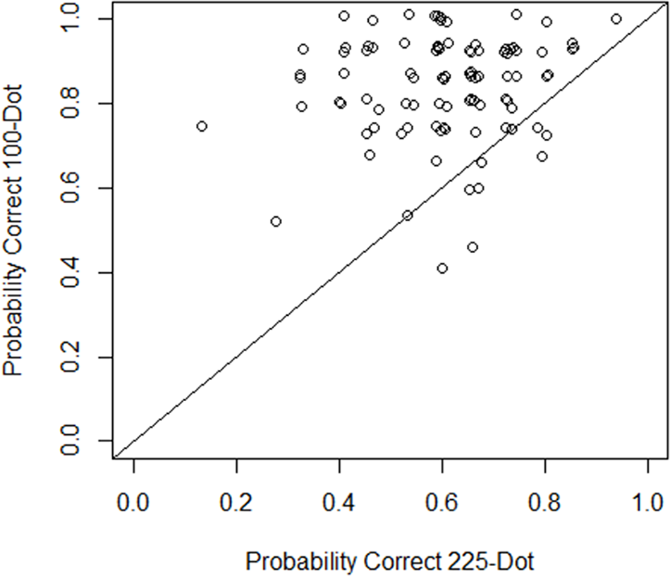

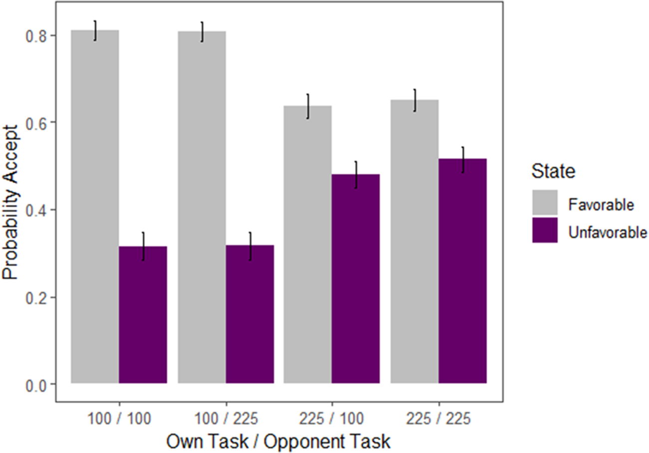


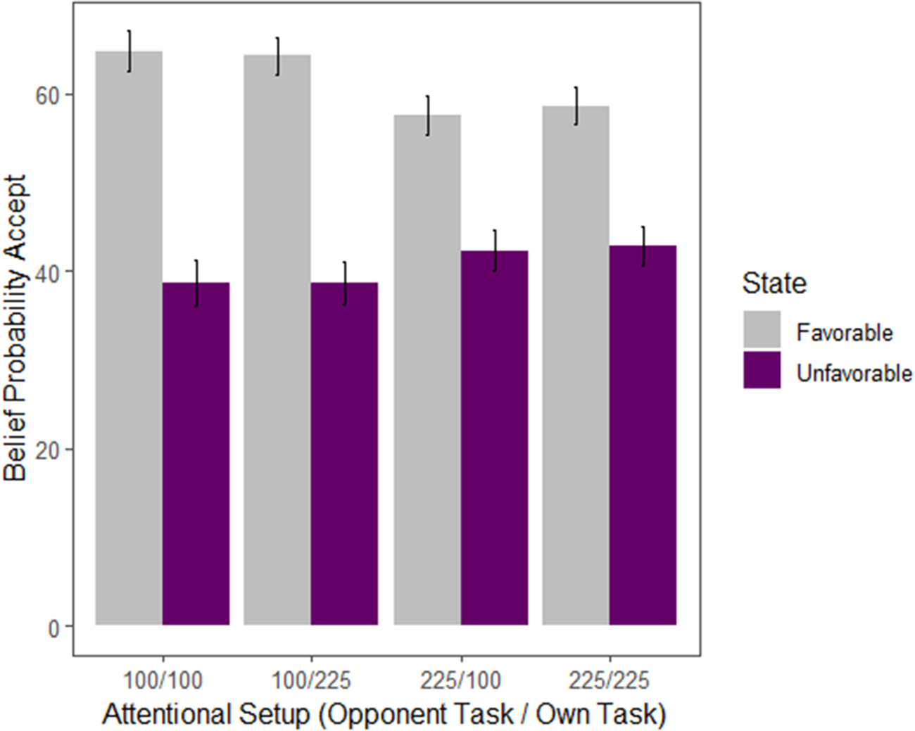


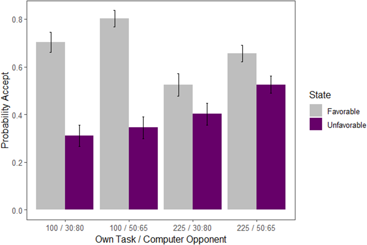


 Open access