

1. Introduction
A satellite radar altimeter transmits pulses towards the sub-satellite point and receives a returned signal which is affected by its reflection at the surface and/or the scattering by the sub-surface. The main information is the time for the pulse to be returned, which gives the height between the surface and the reference ellipsoid. Thus, the primary interest of these measurements is the construction of a very precise surface topography (see for continental ice sheets,Reference Zwally, Bindschadler, Brenner, Martin and Thomas Zwally and others, 1983; Reference McIntyre and DrewryMcIntyre and Drewry, 1984). Reference Remy, Mazzega, Houry, Broussier and MinsterRemy and others (1989) showed that an adapted inverse technique may provide a topography with a sub-metric precision, even with the Seasat data. The altimeter of the future ERS-I European satellite will provide such a topography of continental ice up to lat. 82°S.
However, altimeter data also include other parameters, which are still little explored. Not only could their physical interpretation be useful for other glaciological topics, but also they can provide information about the physics of the altimetric measurements.
Indeed,Reference Ridley and Partington Ridley and Partington (1988) suggested, using average Seasat altimeter wave forms from three small regions of Antarctica, that both volume and surface scatterings affect the signal to variable extents. Recently, Reference Partington, Ridley, Rapley and ZwallyPartington and others (1989) further argued, using average Seasat and Geosat wave forms, that for dry-snow regions, volume scattering dominates the altimetric return. These results are in opposition to previous theoretical and empirical studies which indicate that near-vertical radar returns over dry snow are dominated by surface scattering at the frequency used for radar altimeters (Reference Fung and EomFung and Eom, 1982; Reference MätzlerMatzler, 1987). An empirical study of the radar wave forms is very difficult. As a matter of fact, if the signal is a surface signal, the wave forms are affected both by the pointing angle of the altimeter and by the surface slope: both effects cannot be separated and both parameters are poorly known. The wave forms are also affected by the large-scale undulation curvature (Reference Martin, Zwally, Brenner and BindschadlerMartin and others, 1983) and by the medium-scale features: snow dunes or sastrugi. If the signal is affected by volume scattering, the shape of the wave forms also depends on the dielectric properties of the sub-surface and on the size and density of the scattering particles, both effects also being inseparable (Reference Ridley and PartingtonRidley and Partington, 1988). Too many parameters affect the radar wave forms to allow very firm conclusions on the relative importance of the various effects.
Using Seasat data, the aim of this paper is to study the total energy returned by the surface to the satellite, over continental ice, both to understand better the physics of the scattering, and to interpret the geophysical aspect of the signal. Indeed, we will show that the variations of the intensity of the signal are very large on large distance scales and that only a few parameters can affect it significantly. Operational algorithms used for the estimation of the parameters of the “Geophysical Data Records” and for the control loop of the instrument were designed for the ocean surface. Thus, the return power, as well as the other parameters, first has to be re-estimated directly from the returned pulse wave form.
2. Definition and Correction
a. AGC loop correction
The design of the Seasat altimeter has been given byReference McArthur McArthur (1978). The return wave form of the radar pulse can be seen as the histogram of the return energy, as sampled by a series of 60 gates. Each gate measures the energy during 3.125 ns. The energy return is controlled by an “Automatic Gain Control (AGC) tracking loop” which acts on the transmitted energy intensity, so that the total return energy is maintained as nearly constant: the system estimates the total energy E of the return signal and compares it with a reference level E r. If E is larger than Er the next pulse will be more attenuated, and conversely.
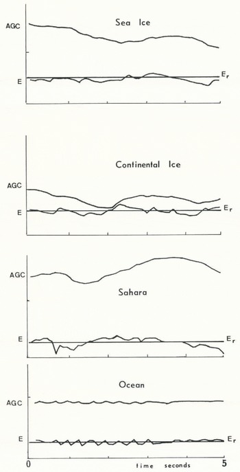
To smooth the AGC sequence and avoid white noise above the ocean, only 1/16 of the correction is applied. Thus, if E and AGC are compared for successive measurements (Fig. 1), it can be verified that E varies around the reference value, depending on the variation of AGC. In the case of the ocean surface, the lag between variations of AGC and variation of E is extremely short. On the contrary, in the case of ice sheets, sea ice, or sand land, the AGC loop only readjusts on time-scales of seconds.
Evolution of the Automatic Gain Control (AGC) and of E the total energy return above sea and continental ice. Sahara, and the ocean during a 5 s interval. The mark on the AGC scale of each diagram is the 30 dB level. The vertical axes have different scales.
To correct for the AGC loop inefficiency, one has to redefine the AGC by keeping constant the total energy of the retracked wave form. We therefore introduce Agc as:
or
The correction to apply to the AGC for estimating the actual energy return is of the order of 2 dB r.m.s.
b. Tracking-system correction
As for AGC, the altimetric height is followed with a height-tracking loop, which takes into account only a small part of the topography: the tracking-loop response is too slow for the strong variations of the ice-sheet topography, and the signal is shifted within the receiving window.
This mispositioning of the return pulse in the receiving window also affects the AGC For example, if the signal is early with respect to the middle of the pre-positioned receiving window, the system will sum up the last gates in excess, E will be too large, and the next AGC value will be adjusted to a larger value. This effect is the same as that introduced by the sea-state bias on the back-scatter coefficient used for measuring wind speeds above the ocean (e.g. Reference Chelton and WentzChelton and Wentz, 1986). A five-gates drift of the tracker introduces a 0.7 dB shift on AGC This is illustrated in Figure 2, which represents a continuous series of altimeter wave forms above Antarctica. In the case of wave forms Nos 10 to 18, it is evidence that the AGC variations are only artefacts, due to the mispositioning of the window with respect to the signal.
Sequence of 0.1 s averages of the return wave form above Antarctica showing the relation between the Agc and the tracker error. The Agc value is given in the upper left corners of the diagrams, expressed in decibels.

The operation for correcting this mispositioning is named retracking. In general, the existing retracking algorithms are designed for surface scattering.Reference Martin, Zwally, Brenner and Bindschadler Martin and others (1983) fitted a theoretical wave form to the 60 gates. This method is very precise but arduous.Reference Brooks, Campbell, Ramseier, Stanley and Zwally Brooks and others (1978) assumed that the energy at the middle of the front edge of the wave form is the half value of the maximum power: this method is very easy, but noisy. More recently, Reference Wingham, Rapley and GriffithsWingham and others (1986) approximated the wave form by a rectangle, chosen to have its centre of gravity and area equal to those of the wave form.
Here, we will use the on-board tracking algorithm:Reference McArthur McArthur (1978) showed that the half-power point on the leading edge of the return pulse is equal to the integral of the total return scaled by 53/60, to compensate for the effect of the antenna diagram (this gate number is currently named the AGC gate number). Then, we have to find the gate the energy of which verifies:

where P R(τ) is the return power of gate τ.
We will see in section 4 that this retracking technique is quite adaptable for surface scattering, and introduces only a sub-decibel error in the case of pure volume scattering.
As the signal is shifted, the calculated sum is not the “true” one; an iterative scheme must be used. A residual drift of one gate, or a height error of 47 cm, leads to a factor error of (1 ± 1/30) on the total return energy, which means a 0.14 dB error on AGC Like the method ofReference Wingham, Rapley and Griffiths Wingham and others (1986), this retracking technique uses all range bins to estimate the retracking position, and the noise on the altimeter-return power is smoothed. This method is very easy to implement and gives direct access to the total energy. Both corrections on AGC (AGC loop and retracking) have been applied to a sector of Antarctica, to a sub-set of Seasat data (Fig. 3). In Figure 4, these AGC′ values are displayed against AGC for 5000 pulses. The r.m.s of the correction is about 2 dB.

Plot of the corrected Automatic Gain Control (AGC′) versus the measured AGC. The r.m.s. difference is 1 db. The gap near 32 dB is probably due to malfunctioning of the instrument.

3. Observations Of AGC From Seasat Data
3.1. Observations along profiles
The data from Figure 3 have been analysed for AGC Figure 5a represents the retracked altimetric height, along a 100 km long path of the Bermuda repeat orbit. The profile shows a large-scale parabolic trend fitted with a polynomial function. 30 km wavelength undulations are superimposed. The altimetric height is reproducible within 50 cm r.m.s., which gives confidence to the retracking technique. The corresponding noise on AGC would be about 0.24 dB r.m.s. Figure 5b represents two repeat AGC profiles for the same track: the pattern is very reproducible within 0.3 dB. It shows a slow decrease of about 2 dB along the arc, with variations on a superimposed 15 km wavelength. These AGC undulations, being reproducible, are probably geophysically significant. At the end of the track, because of an abrupt change in slope, the control loops failed to maintain the signal within the window and the track was interrupted.
(a) Retracked altimetric heights along a 100km long path of the repetitive orbit of Seasat. The smooth curve is a parabolic fit along the profile, (b) Corresponding profiles for AGC.

We further investigated the medium-scale signals by doing a spectral analysis over a longer profile. Figure 6a shows an altimetric height profile for a 300 km long path. As in Figure 5a, the residues relative to a parabolic profile (Fig. 6b) show regular medium-scale undulations, of wavelength 20 km and height amplitude about 5 m. This is clearly visible in the spectral analysis (Fig. 6c). The same analysis has been done for AGC, along the same track. The pattern shows a large-scale signal varying from 24 to 28 dB (Fig. 6d). When this large-scale trend is removed, residues of 1 dB amplitude appear (Fig. 6e), and the spectral analysis (Fig. 6f) shows a 10 km wavelength signal. These medium-scale variations of Agc are probably related to the medium-scale topography. We will explain latter why the wavelength of Agc variations is half that of the topography.
(a) Retracked altimetric height along a 300 km long path, with a parabolic fit superimposed, (b) Residues between altimetric height and the parabolic fit. (c) Spectral analysis of the residues. Note the 20km wavelength undulations, (d), (e), and (f) represent the same treatment for AGC′, for the same path. Note the 10 km wavelength undulations.

3.2. Large-scale AGC observations
The overall variations of AGC for the entire area are of the order of 15 dB around a mean value of 27 dB (Fig. 7). Though the distribution of these values is rather Gaussian, systematic large-scale geographical variations can be observed. Figure 8 represents the distribution of values for two domains, shown in Figure 3. The scatter in each domain is about half that on the large scale: the mean values in each domain are significantly different, of the order of 24 and 28 dB, respectively.
Distribution of the corrected Automatic Gain Control AGC′. m is the average and s the root mean squares.

Distribution of AGC in two domains A and B, represented in Figure 3.

Figure 9 is a map of AGC values. The data have been averaged in 20 × 30 km2 domains, the number of data points in each domain being of the order of 25. The medium-scale signal must vanish after the averaging process. The values vary from 20 to 35 dB. The variations are very smooth. Neither the slope nor the altitude of the superimposed topography seems to be related to the signal. Reference Partington, Ridley, Rapley and ZwallyPartington and others (1989) have already mentioned that no correlation was found between wave form and altitude. If volume scattering is dominant, one would expect a correlation between wave form (or AGC) and temperature (or altitude).
Map of 〈AGC′〉 averaged over 20 × 30 km2 domains. The topographic contours are fromReference Drewry and Drewry Drewry (1983).

In Figure 10, the katabatic wind flow lines (Reference ParishParish, 1982) of this area are superimposed on the 〈AGC〉 map. These winds are stronger where the topography channels them. The case for intense winds near Cape Denison (along long. 140 °E.) is particularly well known (Reference ParishParish, 1982). By eye, it seems that 〈AGC〉 is smaller (of the order of 20 dB) in areas of wind chanelling (near long. 100° and 140°E.) and larger (near 30 dB) in areas of domes and slower wind speeds (near zone B in Figure 3). Note that, although katabatic wind intensity is related to topography, the observed correlation between AGC and wind cannot be explained by an effect of topography on AGC. In particular, the areas where strong katabatic winds are found are concave on a scale larger than 200 km. The altimetric return is sensitive to concavity and slope on the scale of the footprint, of the order of 10 km.
Same as Figure 9 with katabatic flow lines ofReference ParishParish (1982) superimposed. The values are also scaled in quadratic mean slope of the surface as explained in the text.

For quantifying this comparison. Parish’s flow line has been digitized and the wind assumed to be inversely dependent on the flow-line distance. In other words, the flux is assumed to be constant between two flow lines, as defined by Reference ParishParish (1982). In Figure 11, this wind intensity is plotted against the 〈AGC〉 values binned every dB. Seven hundred regions are used. The linear correlation coefficient is 0.56, which is significant at more than the 99% confidence level. We therefore find evidence that the corrected Automatic Gain Control, averaged on a medium scale, is mostly sensitive to wind-induced effects.
Relation between AGC and wind intensity deduced from Reference ParishParish (1982) and averaged for each 1 dB interval of 〈AGC〉.

In order to support a quantitative comparison, one can scale the wind intensity: the wind measurement at Pioneerskaya Station (lat. 69.7°S., long. 95.5°E.) and at Charcot Station (lat. 69.05′S., long. 138.5°E.) is 10 m/s (Reference Kodarna and WendlerKodarna and Wendler, 1986); the corresponding AGCs for both stations are 25 dB. This scaling leads to an average wind intensity in the sector of 7.5 m/ s, corresponding to the average AGC value of 27 dB (Fig. 7). The estimated wind intensity varies between 5 and 25 m/ s, which is consistent with in-situ observations.
One could a priori imagine using these data to provide a map of katabatic wind intensity above Antarctica, and its possible seasonal variations. An approach, not used further here, would be to use the empirical relation between 〈AGC〉 and wind as given in Figure 11. This would integrate all possible physical effects on AGC. Note that this approach would not be different from that used for estimating altimetric winds above the ocean (Reference Chelton and WentzChelton and Wentz, 1986). As this relation is apparently not linear, for a given precision of 〈AGC〉 the sensitivity of the wind determination will be smaller for strong winds than for light winds. This is similar to the case for the ocean.
To understand the physical control of the altimetric return intensity, we now model AGC. The strong observed variations of AGC correspond to variations of the total energy, by a factor 30: a parameter able to provide such a variation must be easily detected after a theoretical analysis.
4. Surface Scattering
4.1. The analytical formulation for AGC
The theoretical model for the wave forms and for their integral will depend on the nature of the scattering. For a surface echo, theReference BrownBrown (1977) model can be used to describe altimeter wave forms. The elements of this model are briefly recalled. For a flat surface, the average return power P r(t) as a function of time t can be written as
The origin of the time corresponds to the middle of the leading edge of the wave form, a and b which depend on the angle θ, between the pointing direction and the surface impact direction, are expressed in Table I. I 0 is the Bessel function of the second kind, and P r(0) can be expressed by
where G is the antenna gain (see Table I).
Definition of the seasat altimeter parameters

σ 0 is the back-scatter cross-section per unit area and K is the system constant defined inReference McArthurMcArthur (1978):
P t being the transmitted power, λ the radar wavelength, and H the satellite range.
If a Gaussian surface roughness is added, the average return is then a convolution of the height probability density function of the specular points with P r(t), which expresses that some part of the signal will come back earlier. One can easily verify that the total energy or the integral of P r(t) is preserved.
The total received energy is then the integral of Equation (4) during the whole window aperture. After replacing a and b by their values (Table I) and developing the Bessel function, one can show that

where 2T is the duration of the receiving window, 60 × 3.125 ns. Note that this equation is similar to the on-board tracking equation for θ 2 = 0. If not, retracking slightly underestimates the altimetric height. One can now write AGC with respect to the physical parameters:
For Seasat, the nominal value of K dB is 20 dB, but a larger value (22 dB) seems to be required (Reference Chelton and McCabeChelton and McCabe, 1985). A is equal to 8.4 if θ is expressed in degrees.
4.2. The effects of the parameters
a. The surface-slope effect
The term A θ 2 is generally named the attitude loss, because for a flat surface like the ocean, θ is only due to the antenna pointing angle, p. p varied from 0° to 0.53° for Seasat and was corrected for through an on–board algorithm. Here, the incidence angle is also dependent on the surface slope i, on the altimeter footprint scale (Fig. 12). In principle, one should also consider the angle due to the Earth’s ellipticity, about 0.15° at the Antarctica latitudes.
The incidence angle is related to i and p by:
As these angles, except Ω, are very small, one can write:
The variations in p are very slow, and can be seen as a constant bias on a profile scale. Reference Drewry, McIntyre and CooperDrewry and others (1985) have provided model continental ice-surface topographies. They first distinguish large-scale features which are described by nearly parabolic dependence of height upon distance; the induced slope is around 0.06° for an average ice-sheet altitude, and vary on a very large scale. On the contrary, the medium-scale features are typically represented by isotropic “bell-shaped mounds” of 10 m elevation and 20 km size; the induced slope varies by more than 0.2°, on a wavelength half that of the topography (the slope vanishes at the bottoms and at the tops of the undulations, and reaches extremes on both flanks).
Geometry of the problem: p is the pointing angle of the antenna relative to the nadir direction, i is the slope of the surface, and θ is the incidence angle. Ω can take any value ill a given area, depending on the variation in local slope (b) or for different passes with differelll pointing or azimuth angles (c).

The total effect, for such values, is a white noise of about 1 or 2 dB amplitude on AGC, and a signal at the half-undulation wavelength of about 0.3 dB (for the given example). The profile shown in Figure 6 belongs to a typical Antarctic region (see Reference Remy, Mazzega, Houry, Broussier and MinsterRemy and others, 1989). The 10 km wavelength signal identified by the spectral analysis of AGC is probably due to the 20 km wavelength undulation signal on the topography. The observed amplitude of 0.23 dB seems to be consistent with the topography.
b. The back-scatter coefficient effect
In the simplest approximations, the back-scatter coefficient for diffuse reflection above a rough surface is (e.g.Reference Barrick Barrick, 1968;Reference Rott Rott, 1984):
where S 2 is the quadratic mean slope of the surface on the radar wavelength scale, and R 2 is the Fresnel reflection coefficient at normal incidence which depends on the dielectric constant:
For dry snow, ε in turn depends only on the snow density ρ (Reference Tiuri, Sihvola, Nyfors and HallikainenTiuri and others, 1984):
As the surface-snow density on continental ice varies from 0.35 to 0.45, we will assume for R a constant value of 0.145.
4.3. Geophysical interpretation
We will show that the medium-scale variations of AGC can be due to slope effect (Equations (8) and (10)), and find evidence that the large-scale variations can be related to S 2 variations.
On the wavelengths of significance for scattering of the radar signal, the literature describes micro-roughness of wavelength 30 cm and height varying from 0.5 to 2 cm (e.g.Reference Poggi Poggi, 1977;Reference Fung and Eom Fung and Eom, 1982). The small-scale roughness, sastrugi, and snow dunes having wavelengths of 6–30 m and heights of 0.5–2 m (Reference Drewry, McIntyre and CooperDrewry and others, 1985), can play a marginal role in S 2.
These small-scale features vary with wind intensity and are related to the surface-roughness parameter used in micrometeorological descriptions of the atmospheric boundary layer (e.g. Reference HolmgrenHolmgren, 1971;Reference Poggi, André, Wendler, Delaunay, Gosink and Kodoma Poggi and others, 1982). As explained byReference Poggi Poggi (1977), for surfaces affected by asperities of constant height, the surface roughness is proportional to this height. The constant of proportionality is about 10, based on the wind-tunnel experiments of Reference Lettau and QuamLettau (1971). The values given by Reference PatersonPaterson (1981) vary between 0.1 mm for new snow to 11 mm for coarse snow with sastrugi. Using Gaussian distribution for micro-roughness, one can calculate that, through S 2 in Equation (11), variations in the back-scatter coefficient due to these features are up to 40 dB.
As an example, we have parameterized the 〈AGC〉 values in terms of the surface roughness as used by micrometeorologists. By neglecting the Α θ 2 term one can deduce S 2 from 〈AGC〉. Its values vary from 10−2 to 10−4. Assuming that the micro-roughness correlation length is 30 cm, this provides the micro-roughness amplitude which varies from 2.7 to 0.5 cm. This is equivalent to a roughness parameter of 2.7–0.5 mm, for an 〈AGC〉 varying from 20 to 35 dB. These values are in good agreement with those derived from the micrometeorological measurements (Reference PatersonPaterson, 1981).
5. Volume Scattering
5.1. The analytical formulation
For the volume scattering, we will use theReference Ridley and Partington Ridley and Partington (1988) model, modified by Reference Partington, Ridley, Rapley and ZwallyPartington and others (1989) to account for the difference between propagation speeds of radiation in snow and air. Some assumptions are required: the snow-pack must be homogeneous within the altimeter footprint, ice grains must be spherical, and only single scattering is considered. The latter assumption may drastically overestimate volume scattering.
The power received at time t is as follows:

where the time origin, t = 0, corresponds to the beginning of the leading edge of the wave form, n is the refractive index of snow, taken as 1.25 (n is the inverse of the root square of the dielectric constant given in Equation (13)); k e, the extinction coefficient, is the sum of the absorption coefficient k a and the scattering coefficient k s. M is defined as follows:
where K is the system constant defined in Equation (6), τ is the gate duration (3.125 ns), and T is the surface-transmission coefficient; it is linked with the Fresnel coefficient, and is close to 1.
Then, the total received energy per unit area (normalized by πНcτ)), is given by integration of Equation (14). By neglecting ct/n compared to H:

where
Expressed in decibels, K′ is equal to 25 dB, if K equals 22 dB. x m is the vertical maximum depth reached by the radar wave. If the radar range in dry snow is equal to 37 cm, x m is then equal to 11m.
5.2. Geophysical interpretation
As already mentioned, the small variations in the dielectric constant (Equation (13)) lead to small variations in
the refractive index or in the transmission coefficient. The uncertainty in the actual behaviour of K a and k s is a serious limitation for the modelling of volume scattering. Yet, in Figure 13, Equation (16) is computed for k a varying from 0 to », and k s from 0.01 to 10 m−1. The variation in the absorption coefficient does not affect the total intensity. Only variations in the scattering coefficient can explain AGC variations. The scattering coefficient is related to snow density and to grain volume: to describe the 15 dB observed AGC signal, variations in k s by a factor of 30 are required.
In the hypothesis of volume scattering. AGC versus scattering coefficient, for different values of the absorption coefficient. Note that one can neglect variations in this latter parameter.

Such variations are supported, neither by direct measurements of the scattering coefficient, as provided by passive microwave observations, nor by direct measurements of the snow parameters.
Reference Rotman, Fisher and StaelinRotman and others (1982) used the properties of the scattering coefficient in the microwave domain to deduce the accumulation rate from passive radiometer observations. They assumed that the accumulation rate is inversely proportional to the snow-grain volume or to the scattering coefficient as measured by passive radiometer observations (Reference ZwallyZwally, 1977). They derived accumulation rates which are consistent with in-situ data within a factor of 2. If the scattering coefficient is sufficiently affected by the wind for explaining the wind versus AGC correlation, this would have a dramatic result: the wind pattern would be directly visible on the map for accumulation rate as deduced from passive radiometer observations, which is not the case.
For obtaining an order of magnitude on the expected variations of the snow-grain volume, we will choose the equation given byReference Comiso, Zwally and SabaComiso and others (1982), and neglect the density dependence.
where the grain-size is in mm. The order of magnitude of the AGC variations could be explained if k s varies from 0.05 to 10 m−1, or grain-size varies from about 0.5 to 2 mm. In this hypothesis, strong winds would induce a grain-size of about 0.5 mm, and a grain-size larger than 2 mm would be found in regions with low wind intensity. Indeed,Reference Colbeck Colbeck (1980) mentioned that wind may break the snow grains, but sparse measurements in Antarctica, at Byrd Station or at Plateau Station (Reference GowGow, 1969) give values between 0.3 and 0.5 mm for the first meter. This would, in both cases, correspond to low values of AGC. Moreover, Reference Narita and MaenoNarita and Maeno (1979), by studying grain-size at Mizuho Station where katabatic winds are very strong, found a
value (0.56 mm) similar to that at Plateau Station, where the wind intensity is low. Up to now, no measurement in the literature points to such large variations in grain-size, on the large scale.
Furthermore, volume scattering cannot explain the AGC variations at the half-wavelength of the medium-scale surface undulations (Fig. 6): volume scattering does not depend on the incidence angle, above all near the vertical. Thus, the effect of the slope on volume scattering is highly unlikely.
Not only are such large observed variations supported with difficulty but also the model leads to low values of AGC, all the more as the single scattering hypothesis overestimates the estimation. However, when the wind is very strong, it is possible that surface scattering vanishes and the altimetric signal could be affected by volume scattering. Let us look at the induced height error on the retracked data.
5.3. Induced error on the retracking technique
By comparing Equation (14) with the total energy given in Equation (16) and dividing by 53, one can deduce the time t, or the corresponding height error induced by our retracking technique. The results are plotted in Figure 14 for different values of k a First, one can demonstrate that л the maximum retracking error, obtained for a zero absorption and a zero scattering is less than 1.37 m. Secondly, for a significant scattering (k s > 0.2, or AGC > 27, i.e. half of the data), the maximum induced error is reached for k a = 0 and is of the order of 40 cm.
Altimetric height error induced by the retracking method used, in the case of pure volume scattering, versus scattering coefficient and for different values of the absorption coefficient. Note that the error is within a meter.

In conclusion, the larger the scattering coefficient, the more the signal comes from the upper snow layer. This is an important remark, because it provides a means for selecting the region where volume scattering does not affect the altimetric surface measurement significantly. Reference Remy, Mazzega, Houry, Broussier and MinsterRemy and others (1989) showed that above Antarctic lakes, where the surface-slope error vanishes, an inverse technique can provide a precision within 50 cm. Then, if one selects regions with AGC greater than 30 dB, one adds less than 10 cm residual error due to the volume-scattering effect.
6. Conclusion
We have analysed the processes which can affect the power return (or its Automatic Gain Control, AGC) of a radar altimeter above continental ice. On the medium scale, we observe variations of the order of few dB, which seem to be due to surface-slope variations. On the large scale, AGC is strongly correlated with katabatic wind intensity.
If surface scattering is dominant, the physical mechanism able to explain the correlation is the micro-roughness and the small-scale wind-induced features. As above the ocean, wind creates these features which decrease the intensity of the surface scattering. A simplified numerical application leads to a micro-roughness parameter, as used by the micrometeorologists, between 2.7 and 0.5 mm, which is consistent with in-situ measurements. Moreover, in this case, the observed correlation between medium-scale AGC variations and local surface slope can be explained theoretically.
In the case of volume scattering, the correlation with wind must be explained by induced variations in grain-size, via the scattering coefficient. The expected grain-size values vary from 0.5 mm for high wind regions to 2 mm for low wind regions. First, this is in contradiction to the observed variations in the scattering coefficient as deduced from passive radiometer observations. Secondly, such an important signal would undoubtedly have been reported in the literature. Also, the medium-scale variations cannot be explained.
We also show that the model values for volume scattering, even though overestimated by the single-scattering hypothesis, are too low to account for the signal when AGC is sufficiently strong. On the other hand, even in the case of pure volume scattering, the signal comes from the upper snow layer, when the intensity of the altimetric return is important. This provides a means for selecting regions for the survey of the ice-sheet topography by radar altimetry: when the AGC is large, the surface as seen by the radar is close to the actual one.
As above the oceans, the altimeter therefore has the potential for measuring the intensity of katabatic winds. In the case of the oceans, the sea surface responds quickly to variations in surface winds, so that the altimeter provides an estimate of the instantaneous wind. On the contrary, above ice sheets, it is expected that micro-roughness or grain-size rather relate to average wind intensities over some period of time. Further improvements in this analysis require observations of height-slope joint probability distribution of the ice surface and of grain-size, and their relations to wind. Such mapping will be achievable with the ERS-1 data over 80% of Antarctica and over all of the Greenland ice sheet. In addition, the instrument tracker of ERS-1 will follow the ice surface better, and it should be possible to estimate 〈AGC〉 with a precision better than 1 dB.


