


1. INTRODUCTION
Wind is the principal erosion mechanism of granular surfaces such as sand or snow, known as aeolian transport. Kok and others (Reference Kok, Parteli, Michaels and Karam2012) provide an overview of the three modes of aeolian transport, creep, saltation and suspension. Creep describes the rolling and sliding of large particles along a surface, without becoming fully airborne (Bagnold, Reference Bagnold1937). Saltation describes the movement of particles along ballistic trajectories following entrainment by the fluid drag or ejection by impacting particles (Bagnold, Reference Bagnold1941); and are often referred to as drifting particles. Suspension describes the process of particles that follow the turbulent motion of eddies and may remain airborne for a long period of time. Suspension is often characterized by the time that the particles are in the air and by the diameter of the particles, which is generally very small (Gillette and Walker, Reference Gillette and Walker1977; Zender and others, Reference Zender, Newman and Torres2003; Miller and others, Reference Miller2006). Aeolian transport is initiated when the winds shear force acting on the bed exceeds a particle entrainment threshold. The threshold between each transport mode is different and largely influenced by the size of the particles, their material properties (cohesion between particles (Schmidt, Reference Schmidt1982) and particle geometry or surface structures (Doorschot and others, Reference Doorschot, Lehning and Vrouwe2004; Clifton and others, Reference Clifton, Rüedi and Lehning2006; Filhol and Sturm, Reference Filhol and Sturm2015)). Aeolian transport induces an evolution of the snow surface morphology. Particles are entrained and transported along the surface. Interactions of particles with other particles alter the surface morphology generating structures such as ripples, sastrugi, dunes or cornices. Given that both sand and snow exhibit similar aeolian surface structures, many studies have focussed on the behaviour of drifting sand particles. However, snow exhibits a number of differences to sand that render it unsatisfactory to use as an analogue for snow studies.
Models of drifting sand and snow often assume a steady flux in equilibrium with a certain (mean) wind speed (Bagnold, Reference Bagnold1941; Kawamura, Reference Kawamura1951; Owen, Reference Owen1964; Dong and others, Reference Dong, Liu, Wang, Zhao and Wang2003). However, recent studies (Groot Zwaaftink and others, Reference Groot Zwaaftink2013; Walter and others, Reference Walter, Horender, Voegeli and Lehning2014) show that this equilibrium is an approximation, particularly for snow. It is shown that snow flux rates are highly unsteady and not coupled to constant wind speeds but rather to wind fluctuations (Paterna and others, Reference Paterna, Crivelli and Lehning2016). Many of the differences observed in mass flux between sand and snow can be attributed to the differences in material properties. For example, Schmidt (Reference Schmidt1980) shows that cohesion forces between snow particles are much larger than gravitational forces, which can explain many of the differences observed in the saltation behaviour between snow and sand.
A large number of studies looked at the numbers of particles drifting in the saltation layer, either in field experiments in alpine regions (Schmidt and others, Reference Schmidt, Meister and Gubler1984; Meister, Reference Meister1987; Gordon and Taylor, Reference Gordon and Taylor2009; Gordon and others, Reference Gordon, Savelyev and Taylor2009; Naaim-Bouvet and others, Reference Naaim-Bouvet, Bellot and Naaim2010, Reference Naaim-Bouvet, Naaim, Bellot and Nishimura2011) or in polar regions (Nishimura and Nemoto, Reference Nishimura and Nemoto2005). Many experiments were performed in cold wind tunnels (Nishimura and others, Reference Nishimura, Sugiura, Nemoto and Maeno1998; Clifton and others, Reference Clifton, Rüedi and Lehning2006) or used a modelling approach. The majority of these studies focussed on the transport of snow in the saltation layer using snow particle counters therefore neglecting the contribution of creep and suspension modes. Studies observing the evolution of snow surface morphology were performed using terrestrial laser scanner (Trujillo and others, Reference Trujillo, Ramrez and Elder2007, Reference Trujillo, Leonard, Maksym and Lehning2016; Grünewald and others, Reference Grünewald, Schirmer, Mott and Lehning2010) or by modelling the saltation and surface erosion (Meister, Reference Meister1988; Pomeroy, Reference Pomeroy1991; Michaux and others, Reference Michaux, Naaim-Bouvet, Naaim, Lehning and Guyomarc'h2002; Doorschot and others, Reference Doorschot, Lehning and Vrouwe2004; Vionnet and others, Reference Vionnet2013; Comola and Lehning, Reference Comola and Lehning2017). In studies using terrestrial laser scans or aerial images, the temporal resolution is coarse, limited to multiple hours or days (before and after a storm or snow fall event). Herein, we discuss the dynamics of snow drifting through surface erosion and deposition captured at high temporal resolutions in a cold wind tunnel. In particular, we provide insights into the relationship between eroded snow surface volume and the number of particles in saltation mode recorded with a Snow Particle Counter (SPC). Furthermore, we examine how temporal scales of surface erosion influence the mass flux maxima and draw conclusions on the spatiotemporal dynamics of the erosion process. The first section introduces the experimental setup, in particular, the novel Kinect sensor developed as a low cost device to scan the snow surface during the experiments. The following section examines the results of this new approach with respect to the dynamics and quantity of the mass flux due to snow surface erosion. We discuss the total set-averaged mass-flux, based on the difference between surface height measurements captured before and after experimental wind tunnel runs, representing the net eroded/deposited snow during experimentation. We then provide observations of the correlation between the integrated particle and surface mass fluxes. This is performed with respect to size if the observed surface area (support area) as well as the saltation length scale used for the formulation of the saltation profile. Finally, we focus on the spectral mass flux distribution with respect to the differences between particle and surface mass flux. Based on these results we discuss the dynamics of surface erosion and how it affects the particle mass flux in the saltation layer.
2. METHODS AND INSTRUMENTATION
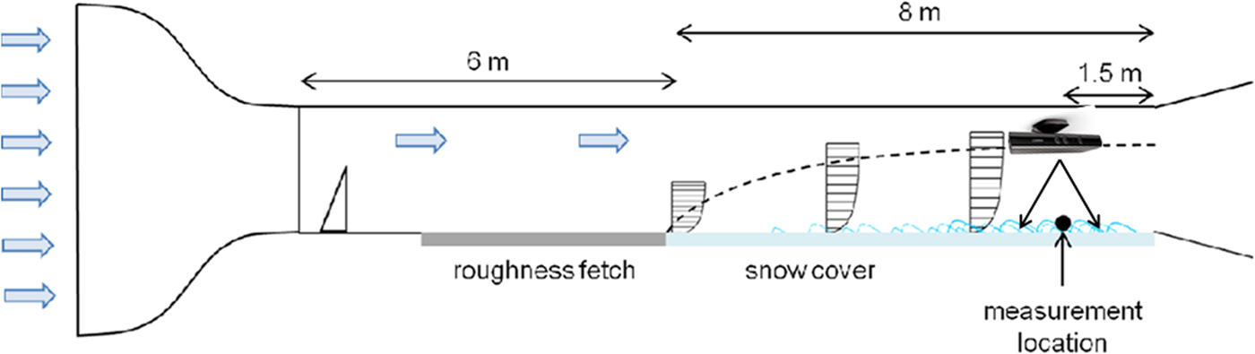
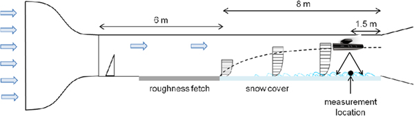
The experiments were conducted in a cold wind tunnel located at 1670 m a.s.l in the Flüela valley near the Snow and Avalanche Research Centre (SLF) in Davos, Switzerland. The tunnel has a 6 m long fetch roughness consisting of a row of spires and roughness elements. Following this, an 8 m long snow cover section completes the tunnel with the measurement instrumentation at the end. The tunnel inlet is composed of a honeycomb grid followed by a 4:1 contraction. The wind tunnel is operated through suction which draws air through the inlet. The snow used during experimentation was natural snow collected in metal trays outside the wind tunnel building. The tunnel was first introduced by Clifton and others (Reference Clifton, Rüedi and Lehning2006). An experiment required a between 0.07 m and 0.15 m of fresh snow (Fig. 1).
Schematic overview of the wind tunnel, including the location of the Kinect device. The Kinect was attached to the wind tunnel ceiling to capture the snow surface change beneath it.
A propeller-type anemometer with an integrated thermometer (MiniAir 20, Schildknecht AG, Switzerland) was used to record the free-stream velocity (U free), the temperature and the relative humidity (RH) in the wind tunnel. Particles in the saltation layer were recorded using the SPC sensor (SPC - S7, Niigata Denki Co.) as first introduced by Nishimura and others (Reference Nishimura, Sugiura, Nemoto and Maeno1998) and Sugiura and others (Reference Sugiura, Nishimura, Maeno and Kimura1998). This method of counting snow particles is based on the voltage change induced as snow particles pass the SPC's photodiode. Based on the amplitude of the voltage signal, a classification of the particle's diameter into 32 size classes between 0.04 and 0.5 mm is possible. The distance between the SPC and the snow surface could be accurately positioned with a traverse stage, which ensured the SPC measurements were taken at a constant 20 mm from the snow surface for each experiment. A drawback of this setup is that particles at the onset of saltation travelling below the height of 20 mm could not be detected. During a number of experiments, saltation below 20 mm was observed to influence snow surface change. Surface erosion (including creep) already starts at low wind speeds close to the threshold wind speed at which the SPC measurements at 20 mm do not record sufficient particles for reliable flux estimates. Addressing this limitation, we applied Microsoft's ‘Kinect for Windows’-device to capture snow surface changes during the experiment. The Kinect was first introduced in 2010 as a low-cost motion sensing input device for a video game console. It consists of an infra red (IR) emitter and sensor, a colour camera, a microphone array and a tilt motor. The sensor module was mounted on the wind tunnel roof using scaffolding. The principal sensor applied in this study was the IR emitter/sensor pair, which captured three-dimensional depth images of the snow surface. Besides the hardware, Microsoft also released a software platform to develop customized software for the Kinect devices. Kinect devices are widely used in other fields such as machine learning (Yavsan and Ucar, Reference Yavsan and Ucar2016) and medical studies (Prochazka and others, Reference Prochazka2016). Mankoff and Russo (Reference Mankoff and Russo2012) discussed possible applications of the Kinect sensor in Earth sciences. Nicholson and others (Reference Nicholson, Pȩtlicki, Partan and MacDonell2016) demonstrate the application of a Kinect device to measure glacial penitentes. One advantage that the Kinect sensor has over traditional photogrammetric setups is that it comes pre-calibrated and does not require reference points (see subsection Kinect mass flux computation).
2.1. Experiments
All experiments presented in this study applied stepped increases of wind speed. Wind speeds started below the threshold for snow particle entrainment and were increased to reach values that induced strong erosion. Between the beginning of January 2016 and March 2016, we performed experiments on 7 separate days. A total number of 115 wind speed steps were recorded. Each step in wind speed lasted ~60 s. The snow density was recorded before experimentation on each test day, and was later used in the surface mass flux calculations.
The Kinect device roof mounting in the wind tunnel oriented the sensors perpendicular to the snow surface. Depth and colour images were recorded using software based on the Kinect Stream Saver application by Dolatabadi and others (Reference Dolatabadi, Taati and Mihailidis2014). The software permitted depth and colour image capture at 30 Hz with a resolution of 640 × 640 pixels. The Kinects field of view (FOV) partly overlapped with the SPC; the pixels containing this overlap were ignored in the analysis. Before recording of each wind step, the height of the SPC was adjusted to 20 mm above the snow surface. This was necessary for each wind step change due to the snow surface erosion incurred during the previous wind step. The threshold freestream velocity U free,t was chosen to be the wind speed at which the SPC was able to detect the first few particles. This point might seem to be a little vague, but it allowed separation between artefacts from the mounting of the snow trays in the wind tunnel and the actual wind-induced erosion.
2.1.1. Kinect mass flux computation
The distance between sensor and snow was below 1 m, which allowed for a 0.90 × 0.68 m sensor footprint that could be evaluated. In the post-processing phase this area was reduced in order to avoid pixel overlap with the area of the SPC. At this range, the Kinect depth sensor precision is 1 mm. The distance between sensor and target determines the resolution in the horizontal field of view (FOV) because the sensor has a set number of pixels. For the experimental setup this gave an average pixel area of ~ 0.3 mm2. Studies looking at the accuracy of the depth sensor (Essmaeel and others, Reference Essmaeel, Gallo, Damiani, De Pietro and Dipanda2014) mention the requirement for data filtering to avoid signal noise. Essmaeel and others (Reference Essmaeel, Gallo, Damiani, De Pietro and Dipanda2012) describe a temporal de-noising filter that addresses this issue. In the present application, the filtering was not required in real-time, it was sufficient to apply it in a post-processing phase. Application of temporal de-noising did not improve data quality in comparison with common moving average filters. Given the Kinects' noisy signal, the time series depth data re-sampled for each pixel from 30 Hz to 1 Hz applying a Savitzky-Golay moving average filter from MATLAB's sgolayfilt function. In addition to the temporal moving average filter, we added a spatial 2-D adaptive noise removal filter (MATLAB's wiener2 function). The wiener2 function was applied to reduce the characteristic Kinect IR noise. After smoothing the time series depth data, they were differentiated to compute the change of the snow surface. This was achieved by calculating the time-derivative for the depth of each pixel, and was applied to the entire event time series. The Kinect device is able to calculate a 3-D coordinate for each pixel using the skeletal stream framework provided in its stream saver software. Within this study, this would have resulted in vast amount of data. Therefore, the post-processing applied a trigonometric approach to calculate the x and y coordinates of each pixel, which was achieved with the following formula:
 $$x_{i,j} = 2{\rm tan}(\beta \cdot (\,j - h/2 + X_o)\cdot z_{i,j})),$$
 $$y_{i,j} = -2{\rm tan}(\alpha \cdot (i - w/2 + Y_o)\cdot z_{i,j}))$$
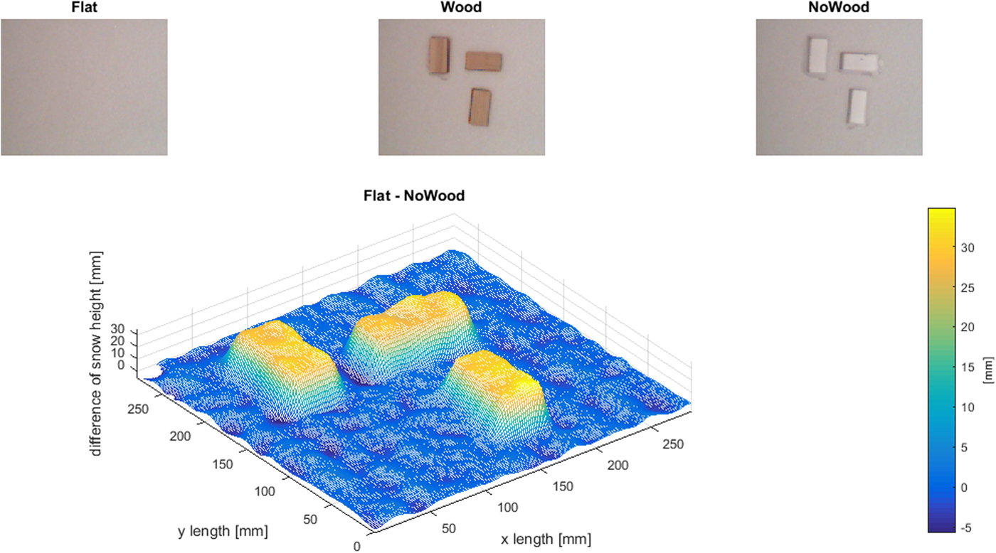
where β is the angle of the depth sensors FOV along the x-direction, and α the angle along y-direction. The calculated angles α and β were validated against the skeletal stream data. X o and Y o represent the offset to the centreline of the FOV in the respective direction. h gives the total number of pixels in the x-direction, and w the total number in y-direction. The symbol i represents the i-th pixel in x-direction, j represents the j-th pixel in y-direction. In order to estimate the quality and precision of the Kinect device, we first conducted a calibration study. The geometrical calibration setup is shown in Figure 2. Firstly, the fresh snow surface was scanned with the Kinect. Following this, three uniform 40mm × 40mm × 80 mm wooden elements were carefully pressed into snow surface creating depressions in the surface, which were then scanned. The snow height difference between each scan provided the calibration required, whereby it was possible to demonstrate that the device measures the correct dimensions of the snow surface and impressions left by the wooden elements. From the calibration tests, we estimated the absolute measurement accuracy of snow depth to be 1 mm. However, by performing the previously described post processing, the uncertainty between consecutive measurements is lower (since the 1 mm precision is averaged to values below 1 mm), as is described by Essmaeel and others (Reference Essmaeel, Gallo, Damiani, De Pietro and Dipanda2012).
Kinect calibration setup. Kinect colour view to the snow with and without wooden elements (upper row). Change of surface height between original snow surface and the snow surface with the impressions of the wooden elements.
The change of volume at each pixel dV i,j was calculated based on the average pixel A i,j area and the change in depth dz i,j
 $$ dV_{i,j} = A_{i,j}\cdot dz_{i,j}.$$
The change of mass per unit area and time for each pixel (mass flux q i,j) is then calculated as the volume changes multiplied by the snow density ρsnow and the time between the time steps as the inverse sampling frequency f s and the total measurement area A
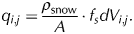 $$q_{i,j} = {\rho_{\rm snow} \over A} \cdot f_s dV_{i,j}.$$
The sum of the mass flux over all pixels divided by the total number of pixels per frame N gives the total surface mass flux q S.
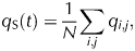 $$q_{\rm S}(t) = {1 \over N}\sum_{i,j}q_{i,j},$$
Integration of the mass flux and mass flux time series by the total run time gives the total time-averaged mass flux Q S.
 $$Q_{\rm S} = \int_{t_0}^{t_{\rm end}} q_{\rm S}(t)\,{\rm d}t$$
In addition to the mass fluxes, we calculated the surface height difference between the first and last frame recorded in a set, which gives the total surface volume change. If the total surface volume change is multiplied by the density of the snow and normalized by the total runtime of the set and surface area, the total set-averaged mass flux Q SB can be obtained. This gives a measure of the total set-averaged mass flux balance. The main difference between the calculations of the time-averaged surface mass flux is the sampling time. In order to observe the influence of the size of the support area, we introduced a reduction factor (RF) with the values 1, 2, 4, 8 and 16. The RF acted as the approximate partition of the initial surface area (i.e. RF=1, no reduction, RF=2, half of a side length and so on). For more details on the RF factor, please refer to the Appendix.
SPC mass flux computation
While the Kinect's depth sensor is able to measure the mass flux based on the change of the snow cover (net vertical flux), the SPC measures the saltation mass flux (horizontal flux) on a small volume in the saltation layer above the snow cover. Following Kawamura (Reference Kawamura1948, Reference Kawamura1951); Dong and Qian (Reference Dong and Qian2007) who express the mass flux profile as an exponential decay; we applied
 $$q_{\rm P}(z) = q_0 \cdot e^{-b \cdot (z-h_0)},$$
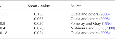
 where q 0 is the average SPC mass flux of the time series at the moment of measurement and h 0 is the height of the SPC measurement above the snow surface. Literature presenting the exponential decay function, for example Rasmussen (Reference Rasmussen1985); Nalpanis and others (Reference Nalpanis, Hunt and Barrett1993); Dong and Qian (Reference Dong and Qian2007), indicate large variability for the parameter b. The parameter b, applied herein, corresponds to the inverse of what is referred to as the saltation system length scale  $L = u_{\ast}^2 / (\lambda g)$ (Guala and others, Reference Guala, Manes, Clifton and Lehning2008). $u_\ast$ is the friction velocity, λ is a constant defining L and g represents the gravitational constant. The value of λ varies in the literature. For calculations presented herein, we applied b based on values by Clifton and others (Reference Clifton, Rüedi and Lehning2006) and Guala and others (Reference Guala, Manes, Clifton and Lehning2008) from experiments performed in the same wind tunnel (L = 0.022). In addition, we performed a sensitivity analysis for values of λ between 0.18 and 1.17 (see appendix, and Table 5) to investigate how λ alters the relation between surface and particle mass flux. As described by Guala and others (Reference Guala, Manes, Clifton and Lehning2008), a small λ extends the height of the saltation layer, where a λ that approaches unity confines the saltation layer close to the surface. The estimation of $u_\ast$ was achieved according to Gromke and others (Reference Gromke, Manes, Walter, Lehning and Guala2011) following the law-of-the-wall, using the averaged free stream wind velocity.
The vertical expansion of the saltation layer was assumed to have a maximal height of z SL = 0.12 m, and corresponded to an estimation based on visual inspections during the experiments. Since previous experiments in the same wind tunnel (Gromke and others, Reference Gromke, Horender, Walter and Lehning2014) reported an exponential decay of the particle number with height, the chosen number seemed reasonable. The mass flux recorded by the SPC is integrated over the total height from z = 0 to z = z SL.
Assuming a linear increase of erosion along the streamwise direction, the divergence of the vertically integrated mass flux profile Q P was calculated. Assuming a linear increase in erosion, the divergence was calculated according to the division of the integrated mass flux by the erosion footprint length L P.
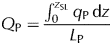 $$Q_{\rm P} = {\int_0^{z_{\rm SL}} q_{\rm P}\,{\rm d}z \over L_{\rm P}}$$
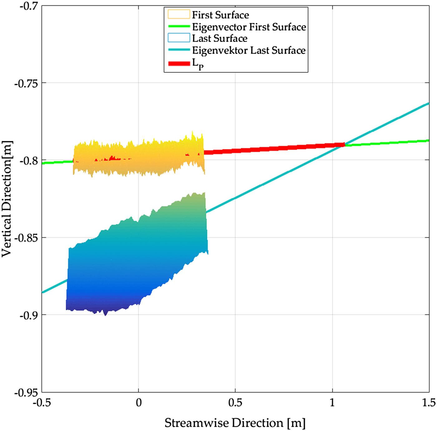
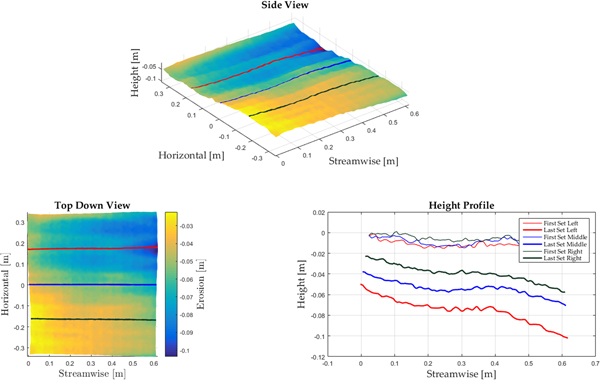
The footprint was estimated as the length before the particle counter at which the snow surface was eroded. In the case of the wind tunnel, where the saltation system develops after a rather short fetch length from zero, the first few metres of the snow surface appeared unchanged after each experiment; independent of snow properties. The calculation of footprint length L P is illustrated in Figure 4. The footprint length corresponds to the length, in which the snow surface is eroded assuming a linear increase of surface erosion with the fetch length. The calculated length L P was in good agreement with the approximate length obtained through visual inspection.
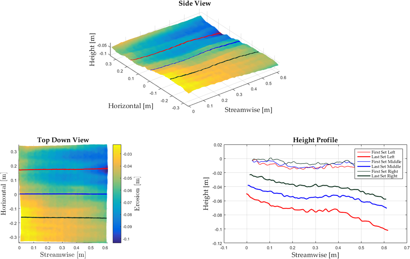
Kinect erosion depth in side view (top), in plan-view (left) and the profiles from before and after a test (right).
Procedure to calculate the saltation footprint length based on the values from Test Day 3. By means of the principal component analysis (PCA) the orthogonal eigenvalues for the snow surface before the experiment (First Surface) and the surface at the end of the experiment (Last Surface) were calculated. Using the two orthogonal, streamwise eigenvectors as well as the difference in height between the untouched surface before and after the end of the experiment, a point of intersection between the two orthogonal vectors could be calculated. The length L P was then given by the distance between the SPC and the point of intersection.
3. RESULTS AND DISCUSSION
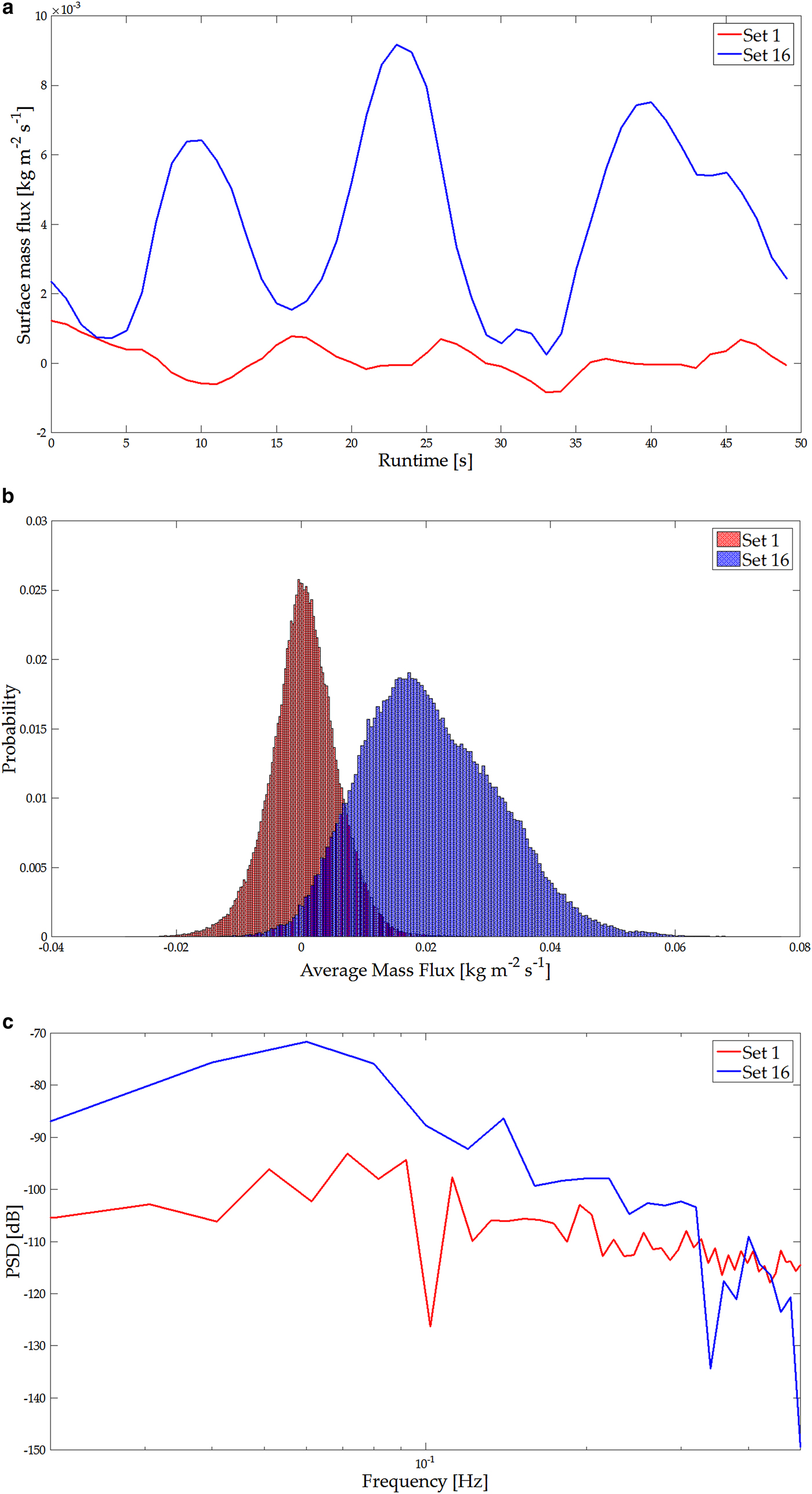
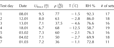
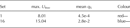
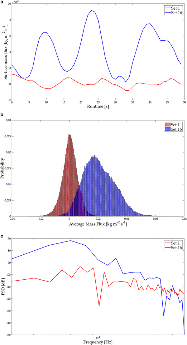
The experimental conditions during this study are summarized in Table 1. Figure 5 displays a representative example of results during a test day that illustrates the dynamics of the surface erosion. Table 2 presents the mean free stream velocity and the net surface mass flux for the two sets in the example. The particle size distribution recorded with the SPC (not shown) for the two sets were very similar. We observed a reduction in the average particle diameter on the individual test days. One process leading to this reduction could be fragmentation of the snow during the tests (Vionnet and others, Reference Vionnet2013). This contradicts the results of Schmidt (Reference Schmidt1981) that the average particle diameter increases with the winds friction velocity. Still we observed an easy entrainment of large particles at low wind speeds on every test day. This may be explained by the fact that large particles initially have more surface area and are therefore more easily entrained. With the given fetch length, the test routine, the duration of the tests and the conditions in the wind tunnel, we expected no significant change in the snow conditions during a test. Particularly from intermediate mass flux strength to high mass flux strengths, little or no diameter reduction was observed. Density changes during erosion have been shown to be small (Sommer and others, Reference Sommer, Lehning and Fierz2018) and therefore we assume constant snow density for the surface flux calculation. The surface flux is of particular interest for the comparison of mass flux through surface erosion with the horizontal particle mass flux. Two time series of the surface mass flux signal recorded with the Kinect device are shown in Fig. 5a. The red line represents a set with low mass flux, the blue line represents a set with high mass flux (see Table 2). The negative values of the mass flux correspond to the accumulation of snow mass, positive mass flux corresponds to erosion. These values in the time series represent the mass flux averaged over the FOV. Higher intermittency in the signal at lower mass fluxes originates from smaller mass flux activity. The red line in Fig. 5a shows a time series of mass flux close to zero. This represents an equilibrium between overall accumulation and erosion in the Kinect's FOV. Although the SPC and the Kinect time series data could be resampled at the same frequency, the processed time series themselves do not correlate well. This is because, the Kinect records temporal dynamics of snow surface erosion, which is not representative of the saltation layer captured by the SPC (refer to Fig. 6). We attribute this to the fact that we averaged the surface mass flux recorded with the Kinect over the whole area of the FOV. Therefore fluctuations in the temporal dynamics of the surface mass flux are smoothed in comparison with the point measurement of mass flux particles in the saltation layer. At the surface, there is not only homogeneous erosion but constant erosion and deposition at different locations such that the mass flux is smoothed. In the case of the horizontal particle mass flux each particle contributes to the mass flux signal independent of the type of surface changes.
(a) Example of time series for two sets with different surface mass flux according to (5). Low mass flux (red) and high mass flux (blue). (b) Histogram of the mass flux for the same two sets. The histogram represents all surface mass flux values for each pixel and time step according to(4). (c) Power spectral density (PSD) for the two time series (for the whole frame again).
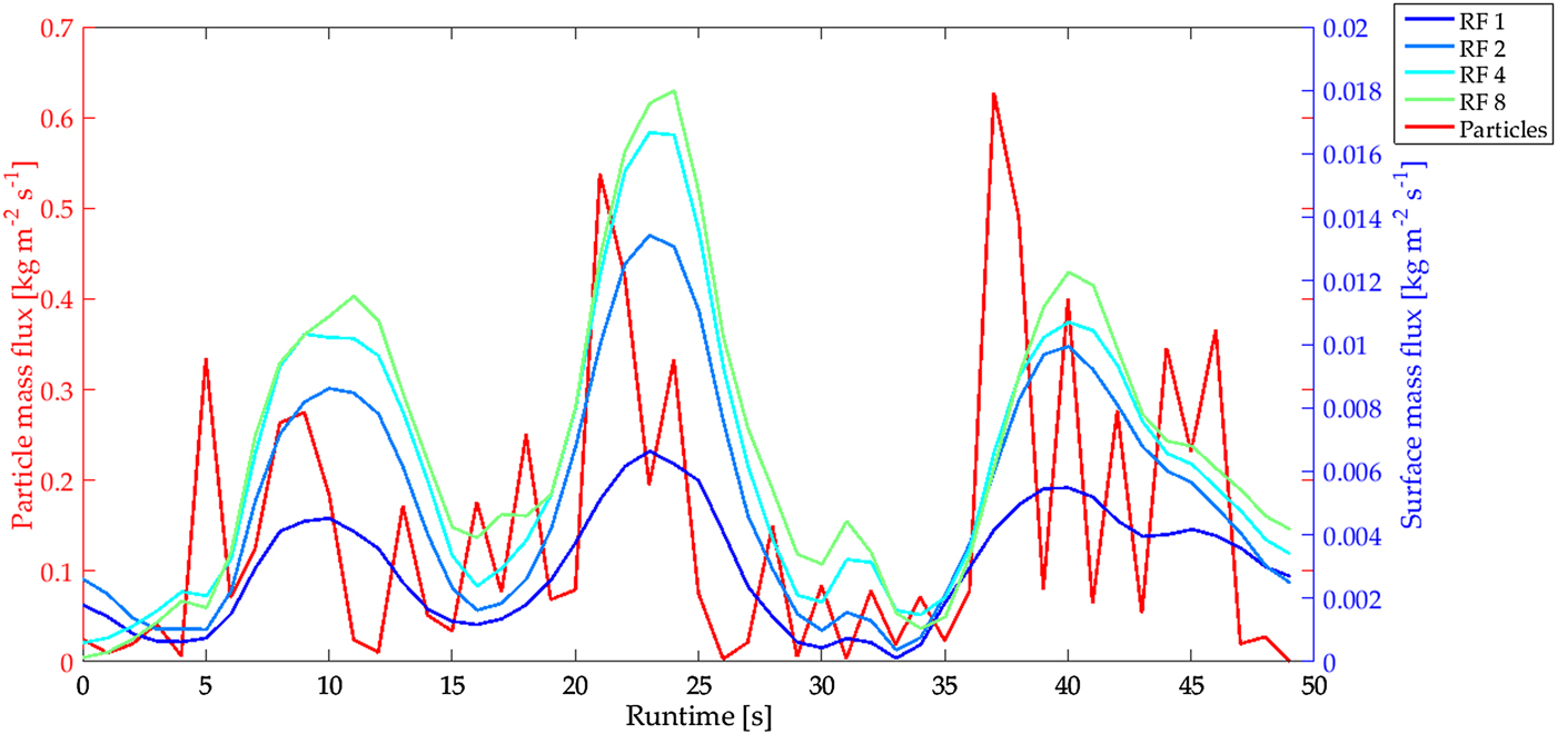
Mass flux time series of set 16 on test day 1. The particles mass flux on the left ordinate (red time series) and the surface mass flux on the right ordinate (blue to green time series) for RF (1, 2, 4, 8) normalized by the corresponding surface area.
Experiments in the winter season 2016
The table provides more details of the two sets displayed in Figure 5. On test day 1 the threshold wind speed at which the particle mass flux recorded with the SPC started was t 9.45 m s −1. Set 1 shows that the surface mass flux that has initiated before transported particles were visible. The units for U free are m s −1, for q S kgm−2s−1
Regarding the averaged mass flux from these time series, the two processes correlate well (refer to Fig. 7). Figure 5a also shows that with increasing free-stream velocity the individual peaks of the time series became both larger in amplitude and longer in period. Thus, strong erosion events induce peak mass flux that lasts much longer in comparison with the mass flux peak of smaller erosion events at lower wind speeds. Paterna and others (Reference Paterna, Crivelli and Lehning2016) revealed that in the wind tunnel, strong saltation developed own saltation length scales independent of the turbulent forcing. These events of strong saltation have their highest power at low frequencies leading to longer lasting bursts of snow particles. Also, in their subsequent study, (Paterna and others, Reference Paterna, Crivelli and Lehning2017) show that in strong saltation peaks of high mass flux persist over a longer time and therefore lead to wider peaks. Figure 5b displays histograms of the mass flux during the two time series from each pixel in the FOV. The results strongly support the previous argument that the equilibrium of erosion and deposition investigated at low mass flux is shifted towards predominantly erosion at high mass flux.
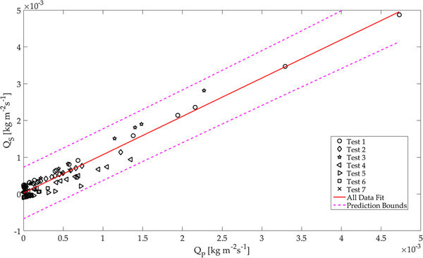
The red line represents the fit for total mass fluxes (Q S vs Q P) of all 115 sets from 7 test days. The different marker represents different test days. The 95% confidence interval as the given by the dashed lines.
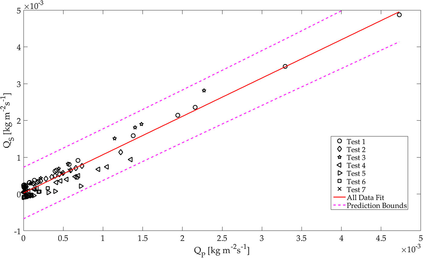
Figure 5c displays the power spectral density (PSD) of the two time series calculated by using MATLAB's pwelch function. The spectral analysis shows differences between equilibrium saltation at low mass flux and erosion dominated saltation, in addition to changes between surface mass flux and particle mass flux. At frequencies close to the sampling frequency (1 Hz), the PSD of high and low mass flux are similar. At low frequencies (below 0.1 Hz), particularly in the case of strong mass flux, the signal contains the strongest power while the power for the low mass flux case is more evenly distributed through the frequencies. This corresponds to what we expected from the observation of wider and longer lasting mass flux peaks of the time series, and is in agreement with the results of Paterna and others (Reference Paterna, Crivelli and Lehning2017).
Figure 6 shows the time series of set 16 (corresponding to the blue lines in the previous figure) observed before (i.e. RF 1) together with the time series of the high mass flux at reduced support areas (RF 2, 4 and 8), as well as the particle mass flux of the SPC for the same set. The magnitude of the surface mass flux increases with decreasing surface area. This increase is based on the fact that the erosion is not uniform in the crosswise direction. Reducing the FOV to the area in the middle of the wind tunnel, areas with less erosion close to the walls are dismissed. Therefore the magnitude increases. This pattern was consistent throughout sets with events of high mass flux on all test days.
This time series further shows that the low-frequency peaks of the surface mass flux correspond well with those of the particle mass flux for all RFs. Furthermore, this is again reflected in the results of Paterna and others (Reference Paterna, Crivelli and Lehning2017) that strong saltation is characterized by long lasting, wide peaks and that the predominant mechanism of entrainment is by splash-entrainment leading to strong erosion.
3.1. Set-averaged and time-averaged mass-flux
As previously stated, we calculated the total, set-averaged surface mass flux Q SB, for each set based on the total mass eroded/deposited within the recording time by subtracting the first surface record in the set from the last of the same set. This way, the temporal information is lost but it becomes possible to compare the integrated particle mass flux profile (Q P, ref. (8)) to the surface change. To compare Q P to Q SB, we calculate their correlation for each set within one test day, as well as the overall correlation for all sets with respects to the reduced surface area (refer to the Appendix A, Table 3). In the case of Q SB for the unreduced surface (i.e. RF = 1), the correlations for the individual events vary largely. Certain events do not correlate (i.e. on test day 6) but some had a very good correlation. Considering all 115 events, the Q SB does correlate with the averaged particle mass flux (r = 0.572). Interestingly, for the case of the reduced support area (RF 2, 4 and 8) the correlation is significantly better (up to r = 0.935 for RF 2 and 4).
Correlation of particle mass flux and set-averaged surface mass flux for different RF
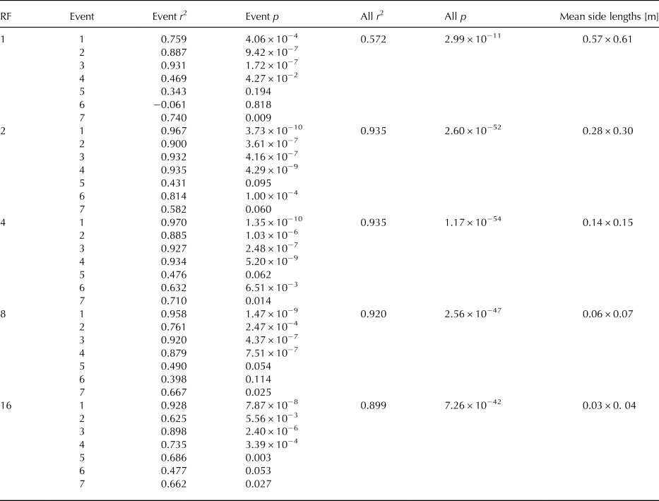
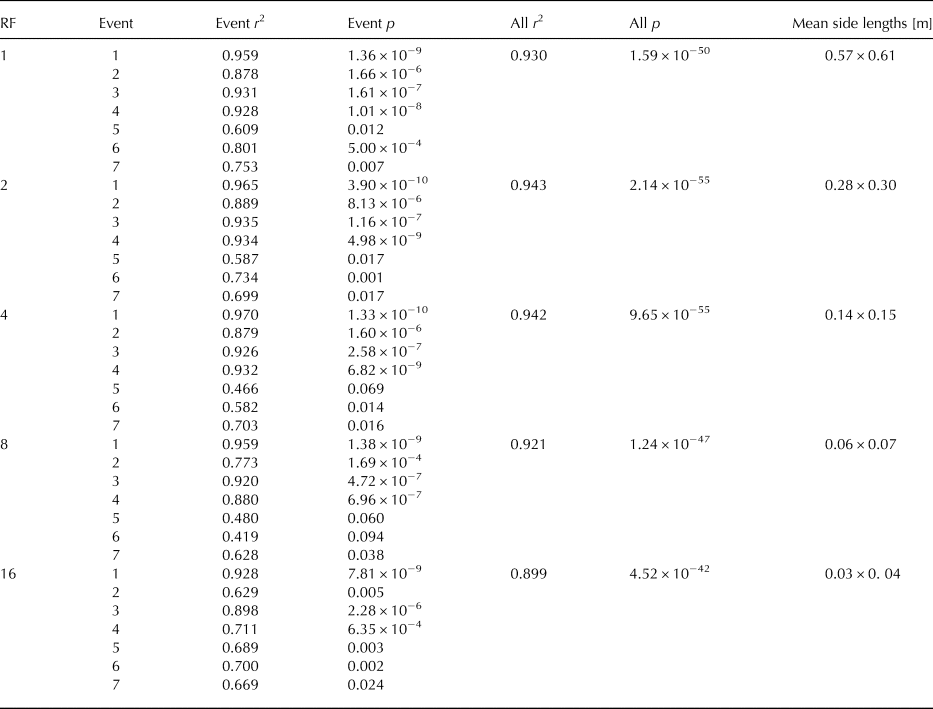
Figure 7 illustrates the correlation analysis between the time-averaged surface mass flux Q S and the integrated particle mass flux profile Q P. Compared with the previous results for the set-averaged surface mass-flux, the time-averaged surface mass flux correlates significantly better (r = 0.930) at the full surface area resolution. The results in the Appendix A and Table 4 again show a higher correlation for the reduced support area (higher than r = 0.94 for RF 2 and 4). Considering the correlation values and more particularly the significance values for both, the set-averaged and the time-averaged mass flux, it demonstrates that the time-averaged mass flux is more robust. This also suggests that the sampling frequency needs to be chosen high enough for a comparison of the two mass fluxes. In both cases, Q SB (Table 3) as well as Q S (Table 4); the smaller support area (i.e. RF = 2 and RF = 4) gives a better correlation. This is because in the case of the reduced surface area, the focus is set on the surface just in front of the particle counter. Another result visible in Figure 7 is that in the case of time-averaged surface mass flux (Q S on the y-axis), the mass flux is near zero for most sets with low and intermediate mass flux strength. This suggests that there is an equilibrium between erosion and deposition similar to what was presented in Figure 5b. This equilibrium shifts towards erosion only (Q S > 0) in the case of stronger mass flux. The parametric study on the saltation-length-scale parameter λ, showed the results were proportional, and therefore the correlation was not influenced significantly. A more interesting observation within that study is the results of linear regressions for the particle mass flux and surface erosion
 $$Q_{\rm S} = p1 Q_{\rm P} + p2.$$
Correlation of particle mass flux and time-averaged surface mass flux for different RF
Values for λ given in the literature and the resulting mean L-value
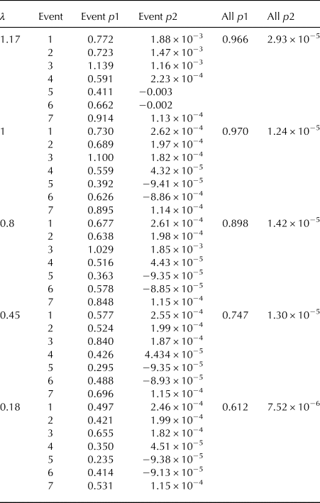
The overview over the results of the regression coefficients p1 and p2 are displayed in the Appendix B, Table 6 for the set-averaged mass flux and Table 7 for the time-averaged mass flux. Looking at the regression coefficient over all events (All p1), we find that in the case of set-averaged mass flux, p1 increases with an increasing λ from 0.676 to 1.069. First, this means that the estimated mass change from the integrated particle mass flux is slightly larger or closely the same as the set-averaged mass flux at the surface. Second, that for a λ with p1 close to one, the integrated particle mass flux is a good estimator of the total change at the surface. Having the best fit at λ = 1 means that for the set-averaged mass-flux, the mass flux profile is confined near to the surface. Notably, in the case of Q SB, the variability in the regression coefficient is relatively high for λ close to one and becomes smaller with a smaller λ. When considering the time-averaged surface mass flux Q S, the relation is very similar (p1 ranges between 0.612 and 0.970), meaning that the time-averaged surface mass flux is slightly smaller than the integrated particle mass flux profile for all five values of λ. Again, the best fit is achieved with λ = 1. This means that by assuming the mass transport closely confined to the surface, the integrated particle mass flux profile best represents the change of mass by erosion and deposition. By comparing the absolute numbers for integrated particle mass flux for λ = 0.18 and λ = 1.17 we show that the latter is significantly smaller. This means in the case of our studies, assuming a high saltation layer overestimates the total integrated particle mass-flux.
Linear regression coefficients for particle mass flux and set-averaged surface mass flux for different λ
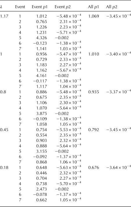
Linear regression coefficients for particle mass flux and time-averaged surface mass flux for different λ
3.2. Spectral distribution
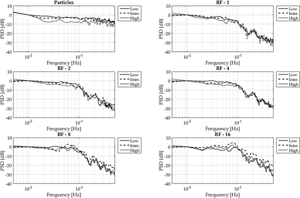
As stated at the beginning of this section, we use the mass flux power spectra to characterize differences between surface and particle mass fluxes. We have already demonstrated with the example in the introduction that there is a difference in the spectrum between high and low mass-flux. Figure 8 shows the spectra over all events for the different RF. All spectra are scaled to their value at 0.01 Hz and averaged in frequency classes of 0.05 Hz. For the subsequent analysis and presentation the sets were separated in low, intermediate and high mass flux based on the time-averaged mass flux strength on the individual test day. Additionally to the spectrum of the surface mass-flux, the spectrum of the particle mass flux was added. It is clear that in the case of the particle mass-flux, the power is evenly distributed through the spectra. However, the surface mass flux has its largest power at low frequencies, which decreases rapidly towards higher frequencies. Another interesting result is that for the low mass flux, there seems to be no relevant difference in the spectra dependent on the RF. For the intermediate mass flux and certainly for the high mass flux, in the region between 3 × 10⁻¹ and 10−1 Hz, the power increases with a decreasing support area. We explain this behaviour based on the fact that for low mass fluxes, the differences between the individual test days are not as large as for the high mass fluxes. Additionally, for low mass flux strengths, we experienced a more homogeneous surface change in the crosswise direction. The higher the wind speeds became, the higher the variability between the RF. A portion of this variability may be influenced by the tunnel sidewalls, although a quantification of this influence was not possible. This crosswise variability is also reflected in the differences of the spectra at depending on the mass flux strength as well as for the support area.
PSD for different RF.
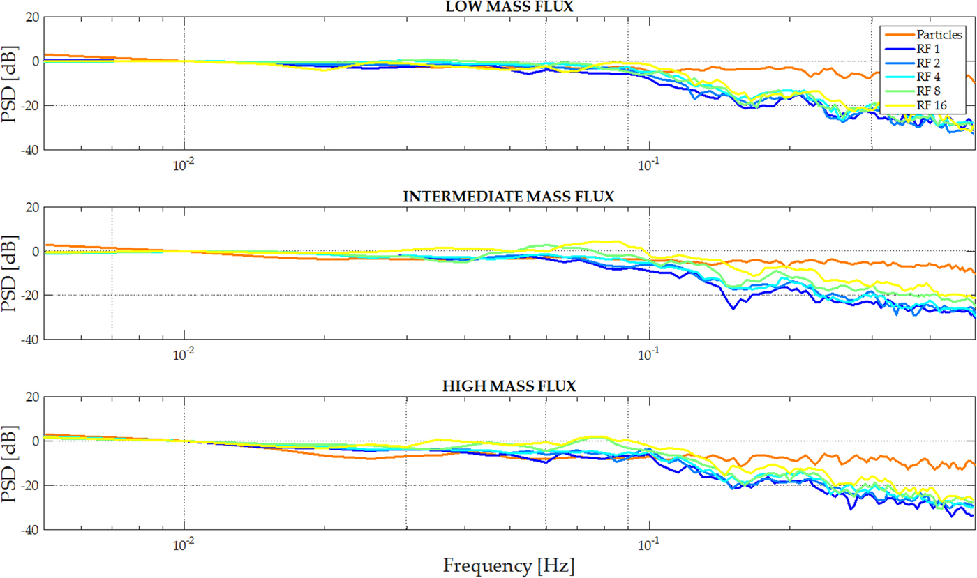
Figure 9 displays the spectra based on the mass flux for the individual surface RF as well as the particle mass flux for all seven test days. As in the previous figure, the PSD for the particle flux is evenly distributed through all frequencies, independent of the mass flux strength. Observing the PSD as a function of the size of the support area, we find that with increasing surface area the power is more evenly distributed in the spectra. That is at RF 1, the gradient of the slope at a frequency of ~ 10−1 is relatively smooth and becomes sharper with increasing RF. We hypothesize that the smoother change at larger observation areas (i.e. RF 1) is because over larger areas, changes due to small-scale events are more smoothed in comparison with smaller observation areas. Unlike the small-scale events at higher frequencies, the slow, larger-scale events of the erosion/deposition occur over the whole FOV and are less dependent on the RF. Therefore, the slow, large events of the erosion/deposition dynamics are more dominant in the spectra.
PSD of high, intermediate and low mass flux, for individual surface RF.
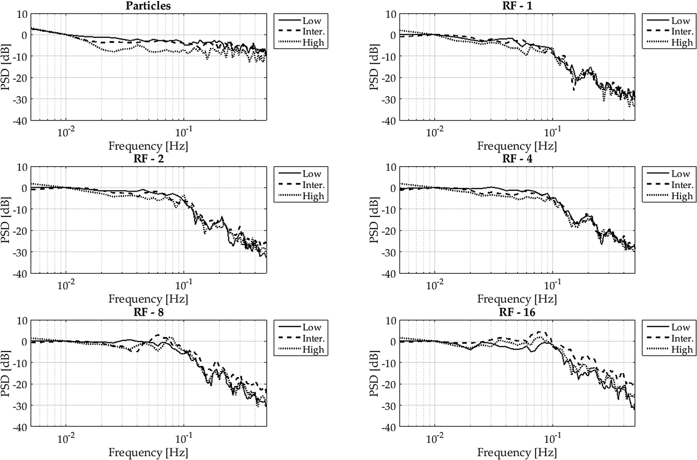
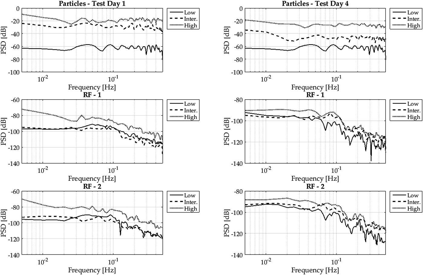
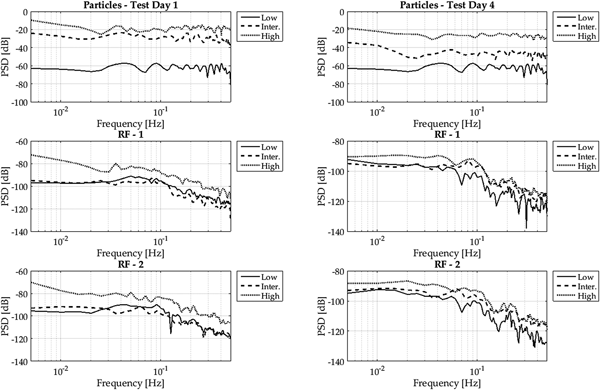
Figure 10 displays the un-normalized spectra for two different test days. On Test day 1, we experienced the highest mass flux. On test day 4, the relative mass flux strength was much smaller. Again the spectra of the particle mass flux look very much alike from their shape. But other than in Figure 8, the unnormalized PSD shows a significant separation of the power dependent on the mass flux strength. Interestingly, for both test days, the power spectra are much closer together for surface mass flux. Still the power is highest for high mass flux, but the gap between high and low mass flux cases is much smaller, particularly at higher frequencies. For the two test days, if the support area is reduced by a factor two, it does not show a significant change in the shape of the PSD. Furthermore, there is no significant separation of the spectra for the intermediate and low mass flux case. Only the shape of the high mass flux case looks different, particularly for test day 1 (which had the strongest mass flux in absolute numbers over all experiments) at low frequencies. This is again in line with the results of Paterna and others (Reference Paterna, Crivelli and Lehning2017) who demonstrate how the duration of events of strong erosion are longer compared with weaker erosion.
Unnormalized PSD for high, intermediate and low mass flux for test day 1 (left column) and test day 4 (right column) for the particle mass flux and RF 1 and 2.
4. CONCLUSIONS
The present study establishes a link between the dynamics of erosion and deposition of snow during snow drifting and blowing at the surface and the snow particles recorded in the saltation layer, applying a newly developed Microsoft Kinect measurement system adapted to a wind tunnel. For the first time, it has been possible to observe and record snow erosion and deposition with a high temporal and spatial resolution. Additionally, it has been possible to measure a quantitative set-averaged mass flux of the total snow mass eroded. A large proportion of the sources of snow transported in the saltation layer can be observed by recording the particle-induced change in the snow surface due to erosion and deposition. Although the accuracy of the Microsoft Kinect is not sufficient to record individual particles, it is possible to record the sum contribution of all particle surface interaction such as deposition at the surface, aerodynamical entrainement or entrainement of particles on the surface due to ‘splash-entrainement’ from impacting particles. During the different experiments a representative variety of snow and environmental conditions were experienced. For the seven test days the threshold wind speed, maximum particle mass flux and snow density were different (see Table 1). We observed equilibrium between erosion and deposition at lower mass fluxes which shifts to predominantly erosion for higher mass fluxes. This study also shows that despite the fact that the temporal dynamics of the mass flux derived from the surface change was significantly different from the particle mass flux in the saltation layer; their average mass flux correlates very well, particularly in case of test day with strong erosion. The correlation can be improved further by reducing the observed snow surface and focussing to a smaller area in front of the SPC. The parametric study for the saltation length scale demonstrated that the best fit between surface mass flux and particle mass flux is achieved for a saltation-length-scale parameter λ close to 1, which translates to a saltation layer that is confined near the surface. The study highlights significant differences in the mass flux between particle saltation and snow surface erosion. The latter has the most power at low frequencies, particularly when considering smaller areas, while the power of the particle mass flux is distributed more evenly through the spectra of the observed frequencies. Despite differences in the characteristic mass flux temporal dynamics, the high correlation suggests that changes of the snow surface are well represented in SPC recordings if long averaging windows are considered. We can therefore conclude that the integrated particles mass flux signal in the saltation layer can be used to quantify the mass eroded on the surface. Furthermore, this would permit estimates of the total mass change to be made from SPC measurements of the particle mass flux only. Readers should consider that this study was performed in a wind tunnel with constant wind speed, which allowed us to control the erosion in the experiments. The limited snow fetch available for snow saltation, an inherent limitation of any wind tunnel experiment, implies that while equilibrium saltation is observed at low mass-flux, at higher mass flux erosion tends to dominate. If a similar study were performed in the field, a much more complex situation would present itself and the results would likewise be influenced by the formation of snow bed forms. It would provide the opportunity to test our results against saltation with a longer flux footprint and under variable wind speeds.
ACKNOWLEDGMENTS
We wish to express our acknowledgment to the Swiss National Science Foundation (SNF) for funding this research (R grant No. 200021-147184) and the wind tunnel facility (REquip grant No. 2160-060998) as well as to James Glover for his effortin writing this article.
APPENDIX A. SURFACE AREA REDUCTION
For each values RF, both side lengths of the observation area were divided through the corresponding number. Therefore the value of RF represent the power of 2 used to reduce the observed surface area of the Kinect. That is RF = 2 means 1/2 of the full side length in streamwise direction and 1/2 of the full side length in crosswise direction. This results in 1/4 of the full surface area used for the mass flux calculation.
APPENDIX B. SALTATION LENGTH SCALE
The saltation length scale  $L = ({u_{\ast}^2})/({\lambda g})$ was introduced earlier in Section 2.1 for the calculation of the particle mass flux profile in the saltation layer. The literature stated different values for the constant parameter λ. Therefore we performed a sensitivity analysis with based on some values given in the literature.







 Open access

