


1 Introduction
Under convex-order-consistent preferences, the classical comonotonic improvement theorem states that every Pareto-optimal allocation of an aggregate loss S among n agents admits a comonotonic representative with the same marginal distributions. The allocation problem therefore collapses to a one-dimensional rearrangement of S. The result was established for expected-utility agents by Borch (Reference Borch1962), extended preference-free by Landsberger and Meilijson (Reference Landsberger and Meilijson1994), and sharpened to integrable aggregate losses on atomless spaces by Ludkovski and Rüschendorf (Reference Ludkovski and Rüschendorf2008). In parallel, the inf-convolution tradition of Barrieu and El Karoui (Reference Barrieu and El Karoui2005), Jouini et al. (Reference Jouini, Schachermayer and Touzi2008), Filipović and Svindland (Reference Filipović and Svindland2008), Acciaio (Reference Acciaio2007), and Rüschendorf (Reference Rüschendorf2013) recasts the problem on spaces of monetary risk measures and identifies convex-order consistency as the structural feature that forces optimal allocations to be comonotonic. The preference class it covers is broad. It contains every law-invariant coherent risk measure (Bäuerle and Müller, Reference Bäuerle and Müller2006), every law-invariant convex risk measure on an atomless space (Jouini et al., Reference Jouini, Schachermayer and Touzi2008), and every distortion risk measure with concave distortion (Wang et al., Reference Wang, Young and Panjer1997), a family that includes Expected Shortfall, spectral risk measures, proportional hazard transforms, and Wang transforms with a concave generator. A parallel to the comonotonic improvement theorem is well known in general equilibrium theory under a different label: in equilibrium, each risk-averse agent’s consumption bundle is nondecreasing in the aggregate endowment so that Pareto-optimal allocations are comonotonic (Mas-Colell et al., Reference Mas-Colell, Whinston and Green1995). Comonotonic reduction is the starting point of most optimal risk-sharing analyses.
In practical situations, risk-sharing problems are rarely unconstrained. Capital regulation imposes ceilings on each entity’s exposure based on its own capital, assets, and reserves. Solvency II (European Commission, 2009) and the Swiss Solvency Test cap one-year changes in own funds through a high-level VaR and ES, respectively. The revised Basel III market-risk framework (BCBS, 2019) replaces the earlier VaR ceiling with an $\mathrm{ES}_{0.975}$
at the trading-desk level. Reinsurance treaties impose capacity limits, quota-share ratios, and excess-of-loss layer caps (Albrecher et al., Reference Albrecher, Beirlant and Teugels2017). Catastrophe bonds and insurance-linked securities introduce attachment points, exhaustion points, and step-up capacities indexed to the aggregate loss (Cummins, Reference Cummins2008). Peer-to-peer pools can cede an upper tail to a reinsurer (Denuit, Reference Denuit2020), and every sharing agreement must satisfy individual rationality so that each agent prefers the pool to walking away (Jouini et al., Reference Jouini, Schachermayer and Touzi2008). Each such arrangement carves out a strict subset of the clearing allocations and raises the question of whether comonotonic reduction still applies.
$\mathrm{ES}_{0.975}$
at the trading-desk level. Reinsurance treaties impose capacity limits, quota-share ratios, and excess-of-loss layer caps (Albrecher et al., Reference Albrecher, Beirlant and Teugels2017). Catastrophe bonds and insurance-linked securities introduce attachment points, exhaustion points, and step-up capacities indexed to the aggregate loss (Cummins, Reference Cummins2008). Peer-to-peer pools can cede an upper tail to a reinsurer (Denuit, Reference Denuit2020), and every sharing agreement must satisfy individual rationality so that each agent prefers the pool to walking away (Jouini et al., Reference Jouini, Schachermayer and Touzi2008). Each such arrangement carves out a strict subset of the clearing allocations and raises the question of whether comonotonic reduction still applies.
We seek a condition on the feasible set that preserves comonotonic reduction under constraints and identify it as componentwise convex-order solidity, the property that every clearing allocation whose components are convex-order dominated by those of a feasible allocation is itself feasible. Informally, making any one agent’s share less risky cannot push the allocation out of the feasible set. Once the feasible set is solid, the classical comonotonic improvement theorem carries over with essentially the same proof; Theorem 2, our constrained comonotonic improvement theorem, reduces to the unconstrained one in a single step. Isolating this property is the substantive step, and it forces the constrained problem back into the geometry where the classical argument applies. In this sense, the result should be read as a constrained-reduction criterion rather than as a new construction of the classical rearrangement. Solidity tells us when a proposed constraint system is compatible with a reduction to comonotonic allocations. A condition for comonotonic allocations is measurability with respect to the total risk S: an allocation that depends on finer state information is not guaranteed to be comonotonic with S. However, constraints that aren’t measurable with respect to S can still admit comonotonic optima in particular problems, since the constraints need not bind at the optimum.
The definition is substantive because it excludes constraints commonly written into regulation and contracts, and this has direct consequences for the structure of the pool and for the incentives facing its participants. Solidity fails in two qualitatively distinct ways. The first arises when feasibility depends on information beyond the aggregate loss. If each agent retains a deductible on its own portfolio, feasibility is driven by each agent’s own portfolio loss, whereas the components of a comonotonic allocation are $\sigma(S)$
-measurable. Optimal allocations then cannot be functions of S alone and must condition on each agent’s individual loss. The second mode arises even when the constraint is
$\sigma(S)$
-measurable. Optimal allocations then cannot be functions of S alone and must condition on each agent’s individual loss. The second mode arises even when the constraint is $\sigma(S)$
-measurable. A VaR ceiling at a fixed level is the canonical example. VaR is not convex-order-consistent, so a firm under such a cap can lower its requirement by splitting its portfolio across subentities and shifting mass into the tail that VaR does not see. Weber (Reference Weber2018) shows that under Solvency II a firm can shrink its VaR capital requirement almost to zero by splitting into enough subentities. This mechanism echoes observations in Xia et al. (Reference Xia, Zou and Hu2023) and resonates with the counter-monotonic quantile-based optima of Embrechts et al. (Reference Embrechts, Liu and Wang2018) and Lauzier et al. (Reference Lauzier, Lin and Wang2023); Lauzier et al. (Reference Lauzier, Lin and Wang2026). Bernard and Tian (Reference Bernard and Tian2009) show that an insurer subject to a VaR regulatory ceiling optimally purchases reinsurance for moderate losses but leaves large losses entirely uninsured, since coverage above the quantile does not affect the binding constraint. This tail-insensitivity of VaR runs directly counter to the purpose of the regulation and reflects the same mechanism that breaks convex-order solidity in our setting. The regulatory incentive therefore points in the opposite direction from a cap based on a convex-order-consistent risk measure: instead of rewarding each agent for flattening the tail of its share, a VaR cap rewards pushing mass further out. Expected Shortfall at the same level dominates VaR and is convex-order-consistent, so replacing the cap with an ES cap at the same level restores solidity. To the best of our knowledge, neither the loss of
$\sigma(S)$
-measurable. A VaR ceiling at a fixed level is the canonical example. VaR is not convex-order-consistent, so a firm under such a cap can lower its requirement by splitting its portfolio across subentities and shifting mass into the tail that VaR does not see. Weber (Reference Weber2018) shows that under Solvency II a firm can shrink its VaR capital requirement almost to zero by splitting into enough subentities. This mechanism echoes observations in Xia et al. (Reference Xia, Zou and Hu2023) and resonates with the counter-monotonic quantile-based optima of Embrechts et al. (Reference Embrechts, Liu and Wang2018) and Lauzier et al. (Reference Lauzier, Lin and Wang2023); Lauzier et al. (Reference Lauzier, Lin and Wang2026). Bernard and Tian (Reference Bernard and Tian2009) show that an insurer subject to a VaR regulatory ceiling optimally purchases reinsurance for moderate losses but leaves large losses entirely uninsured, since coverage above the quantile does not affect the binding constraint. This tail-insensitivity of VaR runs directly counter to the purpose of the regulation and reflects the same mechanism that breaks convex-order solidity in our setting. The regulatory incentive therefore points in the opposite direction from a cap based on a convex-order-consistent risk measure: instead of rewarding each agent for flattening the tail of its share, a VaR cap rewards pushing mass further out. Expected Shortfall at the same level dominates VaR and is convex-order-consistent, so replacing the cap with an ES cap at the same level restores solidity. To the best of our knowledge, neither the loss of $\sigma(S)$
-measurability induced by own-endowment deductibles nor the breakdown of comonotonic reduction under a VaR ceiling with risk-averse decision criteria has been isolated in the prior risk-sharing literature.
$\sigma(S)$
-measurability induced by own-endowment deductibles nor the breakdown of comonotonic reduction under a VaR ceiling with risk-averse decision criteria has been isolated in the prior risk-sharing literature.
On the positive side, solidity admits a broad class of operational constraints: deterministic caps and floors, premium budgets, coherent risk-measure ceilings such as Expected Shortfall, and individual rationality. Solidity is preserved under intersection, so combinations of these are again solid, and the constrained problem admits the same comonotonic reduction as the unconstrained one. Gerber (Reference Gerber1979) extends the Pareto-optimal risk-exchange model of Borch (Reference Borch1962) by allowing non-invasion constraints, and Bühlmann and Jewell (Reference Bühlmann and Jewell1979) incorporate such side constraints into fair Pareto-optimal risk exchanges. Their setting is different from ours: the constraints are tied to individual company losses and payments to other companies, so the optimal exchange need not be determined by the total risk alone, leading to allocations which may not be comonotonic with the total risk. However, in some cases, the optimal constrained allocations are comonotonic with the total risk and recover the same optimal allocation formulas as the risk-exchange model with constraints on the other company’s loss and payment, even if the constraints themselves are not measurable with respect to S. We will expand on this link in Section 6. A complementary thread studies constrained bilateral sharing without a common probability measure. Boonen and Ghossoub (Reference Boonen and Ghossoub2020) consider a decision-maker with subjective expected utility facing a rank-dependent counterparty in a setting with no aggregate loss to share, impose deterministic exposure caps, and obtain optima that are monotone in the likelihood ratio rather than comonotonic. Their failure of comonotonicity is preference-side, driven by heterogeneous beliefs and a nonconvex distortion, whereas our non-comonotonic examples come from the constraint side under shared convex-order-consistent preferences. We fix convex-order-consistent preferences and identify the structural property on the feasible set that preserves the comonotonic reduction.
As a concrete illustration, we revisit the mean-variance risk-sharing problem. In the unconstrained case, the optimum is proportional, with each agent’s share of S tied to that agent’s risk tolerance (Acciaio, Reference Acciaio2007). Under deterministic capacity caps, which are solid, the optimum remains proportional, but only in pieces. Once an agent saturates its capacity, the remaining agents absorb the residual loss in proportion to their own risk tolerances. The sharing rule transitions to a new linear regime at each saturation point and the truncated-affine form shows how a solid constraint reshapes the pool without destroying the comonotonic structure. Replacing the cap with a VaR ceiling at the same level breaks solidity, and we exhibit by example an optimal allocation whose components fail to be comonotonic with S.
The remainder of this paper is structured as follows. Section 2 fixes the setup, introduces the notation, and recalls the unconstrained comonotonic improvement theorem. Section 3 defines componentwise convex-order solidity and proves the constrained comonotonic improvement theorem. Section 4 exhibits three classes of constraints that violate solidity, each yielding an optimal allocation whose components may not be comonotonic with S. Section 5 verifies solidity for the constraint families typically used in practice and discusses a funding-cost adjustment on the objective side. Section 6 applies the constrained reduction to the mean-variance problem.
2 Setup and preliminaries
Let $(\Omega,\mathcal{F},\mathbb{P})$
be an atomless probability space. Each agent
$(\Omega,\mathcal{F},\mathbb{P})$
be an atomless probability space. Each agent $i\in[n]\,:\!=\,\{1,\dots,n\}$
is endowed with a standalone loss
$i\in[n]\,:\!=\,\{1,\dots,n\}$
is endowed with a standalone loss $\zeta_i\in L^1$
, and the aggregate loss shared by the pool is
$\zeta_i\in L^1$
, and the aggregate loss shared by the pool is $S\,:\!=\,\sum_{i=1}^n\zeta_i\in L^1$
. Each agent evaluates losses through a law-invariant risk measure
$S\,:\!=\,\sum_{i=1}^n\zeta_i\in L^1$
. Each agent evaluates losses through a law-invariant risk measure $\rho_i\,:\,L^1\to\mathbb{R}\cup\{+\infty\}$
consistent with risk aversion, in the loss convention where higher values of
$\rho_i\,:\,L^1\to\mathbb{R}\cup\{+\infty\}$
consistent with risk aversion, in the loss convention where higher values of $\rho_i(X_i)$
correspond to worse loss distributions. The unconstrained risk-sharing problem is
$\rho_i(X_i)$
correspond to worse loss distributions. The unconstrained risk-sharing problem is
 \begin{equation}\inf_{\boldsymbol{X}\in\mathbb{A}_n(S)}\sum_{i=1}^n \rho_i(X_i);\qquad\mathbb{A}_n(S)\,:\!=\,\left\{(X_1,\dots,X_n)\in (L^1)^n\,:\, \sum_{i=1}^n X_i=S\ \text{a.s.}\right\}.\end{equation}
The feasible set $\mathbb{A}_n(S)$
collects every clearing allocation of S. Under mild regularity conditions, a minimizer of (1) is Pareto optimal up to deterministic cash transfers between the agents.
$\mathbb{A}_n(S)$
collects every clearing allocation of S. Under mild regularity conditions, a minimizer of (1) is Pareto optimal up to deterministic cash transfers between the agents.
An allocation $\boldsymbol{X}\in\mathbb{A}_n(S)$
is comonotonic with the aggregate loss S if there exist nondecreasing functions
$\boldsymbol{X}\in\mathbb{A}_n(S)$
is comonotonic with the aggregate loss S if there exist nondecreasing functions $f_1,\dots,f_n\,:\,\mathbb{R}\to\mathbb{R}$
with
$f_1,\dots,f_n\,:\,\mathbb{R}\to\mathbb{R}$
with $X_i=f_i(S)$
a.s. for every i and
$X_i=f_i(S)$
a.s. for every i and $\sum_{i=1}^n f_i(s)=s$
for
$\sum_{i=1}^n f_i(s)=s$
for $F_S$
-a.e. s (equivalently,
$F_S$
-a.e. s (equivalently, $\sum_{i=1}^n f_i(S)=S$
a.s.); see Denneberg (Reference Denneberg1994, Proposition 4.5). We denote the set of comonotonic clearing allocations by
$\sum_{i=1}^n f_i(S)=S$
a.s.); see Denneberg (Reference Denneberg1994, Proposition 4.5). We denote the set of comonotonic clearing allocations by
 \begin{equation*}\mathbb{A}_n^{+}(S)\,:\!=\,\left\{\boldsymbol{X}\in\mathbb{A}_n(S)\,:\, X_i=f_i(S)\ \text{a.s. for nondecreasing } f_1,\dots,f_n\,:\,\mathbb{R}\to\mathbb{R}\right\}. \end{equation*}
For any constraint system $\mathbb{C}$
, we define
$\mathbb{C}$
, we define $\mathbb{A}_n^{\mathbb{C}}(S)\,:\!=\,\{\boldsymbol{X}\in\mathbb{A}_n(S)\,:\,\boldsymbol{X}$
satisfies every constraint in
$\mathbb{A}_n^{\mathbb{C}}(S)\,:\!=\,\{\boldsymbol{X}\in\mathbb{A}_n(S)\,:\,\boldsymbol{X}$
satisfies every constraint in $\mathbb{C}\}$
. Let
$\mathbb{C}\}$
. Let
 \begin{equation*}\mathop{\kern.4em\square{}\kern.4em}\limits_{i=1}^{n}\!\!\!_{\mathbb{C}}\rho_i(S)\ \,:\!=\,\ \inf_{\boldsymbol{X}\in\mathbb{A}_n^{\mathbb{C}}(S)}\sum_{i=1}^n\rho_i(X_i)\quad\text{and}\quad\mathop{\kern.4em\boxplus{}\kern.4em}\limits_{i=1}^n\!\!\!_{\mathbb{C}}\rho_i(S)\ \,:\!=\,\ \inf_{\boldsymbol{X}\in\mathbb{A}_n^{\mathbb{C}}(S)\cap\mathbb{A}_n^{+}(S)}\sum_{i=1}^n\rho_i(X_i) \end{equation*}
denote the constrained inf-convolution and its comonotonic restriction, respectively. The unconstrained symbols $\mathop{\square}\nolimits_{i=1}^n\rho_i(S)$
and
$\mathop{\square}\nolimits_{i=1}^n\rho_i(S)$
and $\mathop{\boxplus}\nolimits_{i=1}^n\rho_i(S)$
are obtained by removing the constraint system
$\mathop{\boxplus}\nolimits_{i=1}^n\rho_i(S)$
are obtained by removing the constraint system $\mathbb{C}$
. The unconstrained reduction
$\mathbb{C}$
. The unconstrained reduction $\mathop{\square}\nolimits_{i=1}^n\rho_i(S)=\mathop{\boxplus}\nolimits_{i=1}^n\rho_i(S)$
, recalled in Theorem 1, is what we seek to extend to the constrained setting. The central equality we study is whether
$\mathop{\square}\nolimits_{i=1}^n\rho_i(S)=\mathop{\boxplus}\nolimits_{i=1}^n\rho_i(S)$
, recalled in Theorem 1, is what we seek to extend to the constrained setting. The central equality we study is whether
 \begin{equation}\mathop{\kern.4em\square{}\kern.4em}\limits_{i=1}^n\!\!\!_{\mathbb{C}}\rho_i(S)\;=\;\mathop{\kern.4em\boxplus{}\kern.4em}\limits_{i=1}^n\!\!\!_{\mathbb{C}}\rho_i(S),\end{equation}
where the right-hand side is the same infimum restricted to $\mathbb{A}_n^{\mathbb{C}}(S)\cap\mathbb{A}_n^{+}(S)$
.
$\mathbb{A}_n^{\mathbb{C}}(S)\cap\mathbb{A}_n^{+}(S)$
.
Definition 1 (Pareto optimality). Given a feasible set $\mathcal{X}\subseteq\mathbb{A}_n(S)$
, an allocation
$\mathcal{X}\subseteq\mathbb{A}_n(S)$
, an allocation $\boldsymbol{X}^{\star}\in\mathcal{X}$
is Pareto optimal in
$\boldsymbol{X}^{\star}\in\mathcal{X}$
is Pareto optimal in $\mathcal{X}$
if no
$\mathcal{X}$
if no $\boldsymbol{Y}\in\mathcal{X}$
satisfies
$\boldsymbol{Y}\in\mathcal{X}$
satisfies $\rho_i(Y_i)\le\rho_i(X^{\star}_i)$
for every
$\rho_i(Y_i)\le\rho_i(X^{\star}_i)$
for every $i\in[n]$
with at least one strict inequality.
$i\in[n]$
with at least one strict inequality.
Any minimizer of $\sum_{i=1}^n\rho_i(X_i)$
over
$\sum_{i=1}^n\rho_i(X_i)$
over $\mathcal{X}$
is Pareto optimal in
$\mathcal{X}$
is Pareto optimal in $\mathcal{X}$
.
$\mathcal{X}$
.
2.1 Convex order
The convex order formalizes the notion that one random variable is less dispersed than another while preserving the mean.
Definition 2 (Convex order). For $X,Y\in L^1$
, we write
$X,Y\in L^1$
, we write $Y\le_{\mathrm{cx}} X$
if
$Y\le_{\mathrm{cx}} X$
if $\mathbb{E}[Y]=\mathbb{E}[X]$
and
$\mathbb{E}[Y]=\mathbb{E}[X]$
and $\mathbb{E}[\phi(Y)]\le\mathbb{E}[\phi(X)]$
for every convex
$\mathbb{E}[\phi(Y)]\le\mathbb{E}[\phi(X)]$
for every convex $\phi\,:\,\mathbb{R}\to\mathbb{R}$
.
$\phi\,:\,\mathbb{R}\to\mathbb{R}$
.
Equivalently, $Y\le_{\mathrm{cx}} X$
if and only if
$Y\le_{\mathrm{cx}} X$
if and only if $\mathbb{E}[Y]=\mathbb{E}[X]$
and
$\mathbb{E}[Y]=\mathbb{E}[X]$
and $\int_p^1 F^{-1}_Y(u)\,\mathrm{d} u\le\int_p^1 F^{-1}_X(u)\,\mathrm{d} u$
for every
$\int_p^1 F^{-1}_Y(u)\,\mathrm{d} u\le\int_p^1 F^{-1}_X(u)\,\mathrm{d} u$
for every $p\in[0,1]$
. In the loss convention,
$p\in[0,1]$
. In the loss convention, $Y\le_{\mathrm{cx}} X$
says Y is a mean-preserving contraction of X in the sense of Rothschild and Stiglitz (Reference Rothschild and Stiglitz1970); equivalently, in the wealth convention,
$Y\le_{\mathrm{cx}} X$
says Y is a mean-preserving contraction of X in the sense of Rothschild and Stiglitz (Reference Rothschild and Stiglitz1970); equivalently, in the wealth convention, $-Y$
second-order stochastically dominates
$-Y$
second-order stochastically dominates $-X$
with equal means. Every risk-averse agent with finite mean prefers Y to X.
$-X$
with equal means. Every risk-averse agent with finite mean prefers Y to X.
Assumption 1 (Convex-order-consistent preferences). Each agent’s risk measure $\rho_i\,:\,L^1\to\mathbb{R}\cup\{+\infty\}$
is convex-order-consistent:
$\rho_i\,:\,L^1\to\mathbb{R}\cup\{+\infty\}$
is convex-order-consistent: $Y\le_{\mathrm{cx}} X$
implies
$Y\le_{\mathrm{cx}} X$
implies $\rho_i(Y)\le\rho_i(X)$
.
$\rho_i(Y)\le\rho_i(X)$
.
Throughout we use the extended-arithmetic conventions $a+(+\infty)=+\infty$
for
$a+(+\infty)=+\infty$
for $a\in\mathbb{R}\cup\{+\infty\}$
, and we write
$a\in\mathbb{R}\cup\{+\infty\}$
, and we write $\sum_{i=1}^n\rho_i(X_i)=+\infty$
as soon as
$\sum_{i=1}^n\rho_i(X_i)=+\infty$
as soon as $\rho_i(X_i)=+\infty$
for some i. Infima over empty sets are
$\rho_i(X_i)=+\infty$
for some i. Infima over empty sets are $+\infty$
.
$+\infty$
.
Assumption 1 covers expected concave-utility functionals in the loss convention, that is, $X\mapsto\mathbb{E}[\ell(X)]$
with
$X\mapsto\mathbb{E}[\ell(X)]$
with $\ell$
convex and nondecreasing (equivalently
$\ell$
convex and nondecreasing (equivalently $X\mapsto-\mathbb{E}[u(-X)]$
for concave u, where
$X\mapsto-\mathbb{E}[u(-X)]$
for concave u, where $-X$
is the wealth representation). Here, law-invariance means the risk measure assigns the same value to losses with the same distribution, convex-order consistency means monotonicity under mean-preserving contractions, and coherence refers to the usual axioms of monotonicity, cash additivity, positive homogeneity, and subadditivity. It also covers law-invariant coherent risk measures (Bäuerle and Müller, Reference Bäuerle and Müller2006), distortion risk measures with concave distortion (Wang et al., Reference Wang, Young and Panjer1997), and law-invariant convex monetary risk measures on atomless probability spaces (Jouini et al., Reference Jouini, Schachermayer and Touzi2008), under the standard regularity conditions on the underlying function space that render these classes convex-order-consistent.
$-X$
is the wealth representation). Here, law-invariance means the risk measure assigns the same value to losses with the same distribution, convex-order consistency means monotonicity under mean-preserving contractions, and coherence refers to the usual axioms of monotonicity, cash additivity, positive homogeneity, and subadditivity. It also covers law-invariant coherent risk measures (Bäuerle and Müller, Reference Bäuerle and Müller2006), distortion risk measures with concave distortion (Wang et al., Reference Wang, Young and Panjer1997), and law-invariant convex monetary risk measures on atomless probability spaces (Jouini et al., Reference Jouini, Schachermayer and Touzi2008), under the standard regularity conditions on the underlying function space that render these classes convex-order-consistent.
Throughout the paper, $\mathrm{VaR}_\alpha$
denotes the lower
$\mathrm{VaR}_\alpha$
denotes the lower $\alpha$
-quantile,
$\alpha$
-quantile, $\mathrm{VaR}_\alpha(X)\,:\!=\,\inf\{x\in\mathbb{R}\,:\,\mathbb{P}(X\le x)\ge\alpha\}$
, for
$\mathrm{VaR}_\alpha(X)\,:\!=\,\inf\{x\in\mathbb{R}\,:\,\mathbb{P}(X\le x)\ge\alpha\}$
, for $\alpha\in(0,1)$
.
$\alpha\in(0,1)$
.
2.2 Unconstrained comonotonic improvement
The following is the comonotonic improvement theorem of Ludkovski and Rüschendorf (Reference Ludkovski and Rüschendorf2008), which extends to integrable aggregate losses the construction of Landsberger and Meilijson (Reference Landsberger and Meilijson1994) for the bounded discrete case. The original statements are phrased in terms of a stop-loss order; for $L^1$
aggregate losses with equal means, this coincides with the convex order used here.
$L^1$
aggregate losses with equal means, this coincides with the convex order used here.
Theorem 1.
Let $(\Omega,\mathcal{F},\mathbb{P})$
be atomless and
$(\Omega,\mathcal{F},\mathbb{P})$
be atomless and $S\in L^1$
. For every
$S\in L^1$
. For every $\boldsymbol{X}=(X_1,\dots,X_n)\in\mathbb{A}_n(S)$
, there exists
$\boldsymbol{X}=(X_1,\dots,X_n)\in\mathbb{A}_n(S)$
, there exists $\bar{\boldsymbol{X}}=(\bar X_1,\dots,\bar X_n)\in\mathbb{A}_n^{+}(S)$
such that
$\bar{\boldsymbol{X}}=(\bar X_1,\dots,\bar X_n)\in\mathbb{A}_n^{+}(S)$
such that $\bar X_i\le_{\mathrm{cx}} X_i$
for every
$\bar X_i\le_{\mathrm{cx}} X_i$
for every $i\in[n]$
.
$i\in[n]$
.
Comonotonicity also has a desirable incentive interpretation, sometimes called the no-sabotage property. If $\boldsymbol{X}\in\mathbb{A}_n^{+}(S)$
, so each share is a nondecreasing function of the aggregate loss
$\boldsymbol{X}\in\mathbb{A}_n^{+}(S)$
, so each share is a nondecreasing function of the aggregate loss $X_i=f_i(S)$
, then an agent cannot reduce its own allocation by secretly inflating its own contribution to S, since a larger S weakly increases every
$X_i=f_i(S)$
, then an agent cannot reduce its own allocation by secretly inflating its own contribution to S, since a larger S weakly increases every $X_i$
. See Carlier and Dana (Reference Carlier and Dana2003) for further discussion of this property and its economic relevance. Non-comonotonic allocations generally lack this stability property.
$X_i$
. See Carlier and Dana (Reference Carlier and Dana2003) for further discussion of this property and its economic relevance. Non-comonotonic allocations generally lack this stability property.
Remark 1. Two features of the comonotonic improvement are relevant to Section 3. First, it is componentwise: $\bar X_i\le_{\mathrm{cx}} X_i$
holds separately for each i, with no cross-component comparison. Second, it is law-based:
$\bar X_i\le_{\mathrm{cx}} X_i$
holds separately for each i, with no cross-component comparison. Second, it is law-based: $\bar X_i\le_{\mathrm{cx}} X_i$
compares the marginal distributions of
$\bar X_i\le_{\mathrm{cx}} X_i$
compares the marginal distributions of $\bar X_i$
and
$\bar X_i$
and $X_i$
alone and imposes no restriction on their pathwise coupling. Both features are preserved by feasibility constraints expressed through componentwise convex-order-consistent functionals of each
$X_i$
alone and imposes no restriction on their pathwise coupling. Both features are preserved by feasibility constraints expressed through componentwise convex-order-consistent functionals of each $X_i$
.
$X_i$
.
3 The constrained comonotonic improvement theorem
This section identifies the structural condition on the feasible set under which the unconstrained comonotonic improvement theorem remains valid. We first introduce componentwise convex-order solidity as a property of the constrained feasible set and then state and prove the constrained comonotonic improvement theorem.
3.1 Componentwise convex-order solidity
The comonotonic improvement in Theorem 1 replaces each component $X_i$
by a convex-order smaller
$X_i$
by a convex-order smaller $\bar X_i$
. What a feasible set must tolerate for the comonotonic improvement to stay inside it is therefore exactly this operation: any componentwise convex-order reduction of a feasible allocation should remain feasible.
$\bar X_i$
. What a feasible set must tolerate for the comonotonic improvement to stay inside it is therefore exactly this operation: any componentwise convex-order reduction of a feasible allocation should remain feasible.
Definition 3 (Componentwise convex-order-solid feasible set). A feasible set $\mathcal{X}\subseteq\mathbb{A}_n(S)$
is componentwise convex-order-solid if, for every
$\mathcal{X}\subseteq\mathbb{A}_n(S)$
is componentwise convex-order-solid if, for every $\boldsymbol{X}\in\mathcal{X}$
and every
$\boldsymbol{X}\in\mathcal{X}$
and every $\boldsymbol{Y}\in\mathbb{A}_n(S)$
,
$\boldsymbol{Y}\in\mathbb{A}_n(S)$
,
 \begin{equation*}Y_i\le_{\mathrm{cx}} X_i\, \text{ for every } i\in[n]\quad\Longrightarrow\quad \boldsymbol{Y}\in\mathcal{X}. \end{equation*}
Solidity ensures that the comonotonic rearrangement of Theorem 1, which replaces each component by a convex-order smaller one, cannot leave the feasible set. The condition is componentwise in convex order but joint through the clearing constraint $\boldsymbol{Y}\in\mathbb{A}_n(S)$
, and it is preference-free, in that the reduction applies to every convex-order-consistent preference family once
$\boldsymbol{Y}\in\mathbb{A}_n(S)$
, and it is preference-free, in that the reduction applies to every convex-order-consistent preference family once $\mathcal{X}$
is solid. Solidity is also preserved under arbitrary intersections, by direct verification of Definition 3. Marginal constraints are compatible only when their admissible marginal sets are downward closed in convex order; in particular, ceilings based on convex-order-consistent law-invariant functionals are compatible, whereas law-invariance alone is not enough, with Value-at-Risk ceilings in Section 4 as the canonical counterexample. By contrast, constraints coupling
$\mathcal{X}$
is solid. Solidity is also preserved under arbitrary intersections, by direct verification of Definition 3. Marginal constraints are compatible only when their admissible marginal sets are downward closed in convex order; in particular, ceilings based on convex-order-consistent law-invariant functionals are compatible, whereas law-invariance alone is not enough, with Value-at-Risk ceilings in Section 4 as the canonical counterexample. By contrast, constraints coupling $X_i$
to variables outside
$X_i$
to variables outside $\sigma(S)$
are typically not compatible. Section 4 exhibits three failure modes, and Section 5 catalogues the admissible families.
$\sigma(S)$
are typically not compatible. Section 4 exhibits three failure modes, and Section 5 catalogues the admissible families.
3.2 The constrained comonotonic improvement theorem
The main result of this paper shows that componentwise convex-order solidity is sufficient for the comonotonic improvement in Theorem 1 to remain within the feasible set.
Theorem 2. Let $(\Omega,\mathcal{F},\mathbb{P})$
be atomless, let
$(\Omega,\mathcal{F},\mathbb{P})$
be atomless, let $S\in L^1$
, and let
$S\in L^1$
, and let $\mathcal{X}\subseteq\mathbb{A}_n(S)$
be nonempty and componentwise convex-order-solid. Then:
$\mathcal{X}\subseteq\mathbb{A}_n(S)$
be nonempty and componentwise convex-order-solid. Then:
-
(i) for every $\boldsymbol{X}\in\mathcal{X}$
, there exists a comonotonic allocation
$\bar{\boldsymbol{X}}\in\mathcal{X}\cap\mathbb{A}_n^{+}(S)$
with
$\bar X_i\le_{\mathrm{cx}} X_i$
for every
$i\in[n]$
;
$\boldsymbol{X}\in\mathcal{X}$
, there exists a comonotonic allocation
$\bar{\boldsymbol{X}}\in\mathcal{X}\cap\mathbb{A}_n^{+}(S)$
with
$\bar X_i\le_{\mathrm{cx}} X_i$
for every
$i\in[n]$
; -
(ii) if
$\rho_1,\dots,\rho_n$
satisfy Assumption 1, then (3)
\begin{equation}\inf_{\boldsymbol{X}\in\mathcal{X}}\sum_{i=1}^n\rho_i(X_i)\ =\ \inf_{\boldsymbol{X}\in\mathcal{X}\cap\mathbb{A}_n^{+}(S)}\sum_{i=1}^n\rho_i(X_i);\end{equation}
-
(iii) under Assumption 1, if
$\boldsymbol{X}^{\star}\in\mathcal{X}$
is Pareto optimal, then there exists
$\bar{\boldsymbol{X}}^{\star}\in\mathcal{X}\cap\mathbb{A}_n^{+}(S)$
with
$\rho_i(\bar X^{\star}_i)=\rho_i(X^{\star}_i)$
for every i.






Proof. Fix $\boldsymbol{X}\in\mathcal{X}$
. By Theorem 1, there is
$\boldsymbol{X}\in\mathcal{X}$
. By Theorem 1, there is $\bar{\boldsymbol{X}}\in\mathbb{A}_n^{+}(S)$
with
$\bar{\boldsymbol{X}}\in\mathbb{A}_n^{+}(S)$
with $\bar X_i\le_{\mathrm{cx}} X_i$
for every i. Componentwise convex-order solidity of
$\bar X_i\le_{\mathrm{cx}} X_i$
for every i. Componentwise convex-order solidity of $\mathcal{X}$
gives
$\mathcal{X}$
gives $\bar{\boldsymbol{X}}\in\mathcal{X}$
, proving (i).
$\bar{\boldsymbol{X}}\in\mathcal{X}$
, proving (i).
For (ii), the inequality “ $\le$
” follows from
$\le$
” follows from $\mathcal{X}\cap\mathbb{A}_n^{+}(S)\subseteq\mathcal{X}$
. The reverse inequality follows from (i) and Assumption 1:
$\mathcal{X}\cap\mathbb{A}_n^{+}(S)\subseteq\mathcal{X}$
. The reverse inequality follows from (i) and Assumption 1: $\sum_i\rho_i(\bar X_i)\le\sum_i\rho_i(X_i)$
for every
$\sum_i\rho_i(\bar X_i)\le\sum_i\rho_i(X_i)$
for every $\boldsymbol{X}\in\mathcal{X}$
.
$\boldsymbol{X}\in\mathcal{X}$
.
For (iii), apply (i) to $\boldsymbol{X}^\star$
. Assumption 1 gives
$\boldsymbol{X}^\star$
. Assumption 1 gives $\rho_i(\bar X^\star_i)\le\rho_i(X^\star_i)$
for every i, and Pareto optimality rules out any strict inequality.
$\rho_i(\bar X^\star_i)\le\rho_i(X^\star_i)$
for every i, and Pareto optimality rules out any strict inequality.
Theorem 2 provides a direct recipe: to justify the reduction to the comonotonic subclass on a constrained problem, one verifies componentwise convex-order solidity of the feasible set, which decomposes over intersection; see Section 3.1. Section 5 carries this out for the constraint families typically used in practice. When solidity fails, the comonotonic restriction still returns an upper bound on the constrained inf-convolution, but the bound may be strict. Solidity is sufficient for Theorem 2 but not necessary. A nonsolid feasible set can still admit a comonotonic optimum.
4 Constraints that preclude comonotonic reduction
Three examples show how comonotonic reduction can fail. Section 4.1 shows that constraints coupling $X_i$
with state variables outside
$X_i$
with state variables outside $\sigma(S)$
, such as an agent’s own deductible, which is measurable with respect to its individual loss, need not be admissible. Section 4.2 shows that
$\sigma(S)$
, such as an agent’s own deductible, which is measurable with respect to its individual loss, need not be admissible. Section 4.2 shows that $\sigma(S)$
-measurability combined with monotonicity in S is not sufficient either: a fixed retention plus a catastrophe-only capacity top-up produces a strict gap in (2) under Expected Shortfall objectives. Section 4.3 shows that a Value-at-Risk ceiling produces a strict gap even when the initial endowments are comonotonic and feasible.
$\sigma(S)$
-measurability combined with monotonicity in S is not sufficient either: a fixed retention plus a catastrophe-only capacity top-up produces a strict gap in (2) under Expected Shortfall objectives. Section 4.3 shows that a Value-at-Risk ceiling produces a strict gap even when the initial endowments are comonotonic and feasible.
4.1 Private deductibles on idiosyncratic state
Consider an agent i that contributes its own portfolio of exposures to the pool. Retention rules in practice are defined on the agent’s own portfolio, so the feasibility constraint carries information beyond the aggregate loss. We model this by a deterministic deductible $d_i$
together with a retention rule that references the agent’s idiosyncratic endowment
$d_i$
together with a retention rule that references the agent’s idiosyncratic endowment $\zeta_i$
. Formally, the constraint
$\zeta_i$
. Formally, the constraint $X_i=\zeta_i$
on
$X_i=\zeta_i$
on $\{\zeta_i\lt d_i\}$
and
$\{\zeta_i\lt d_i\}$
and $X_i\ge d_i$
on
$X_i\ge d_i$
on $\{\zeta_i\ge d_i\}$
is measurable with respect to the idiosyncratic
$\{\zeta_i\ge d_i\}$
is measurable with respect to the idiosyncratic $\sigma$
-algebra
$\sigma$
-algebra $\mathcal{G}_i\,:\!=\,\sigma(\zeta_i)$
. When
$\mathcal{G}_i\,:\!=\,\sigma(\zeta_i)$
. When $\sigma(S)\subsetneq\sigma(S,\zeta_i)$
, that is, when
$\sigma(S)\subsetneq\sigma(S,\zeta_i)$
, that is, when $\zeta_i$
is not a function of S alone, the constraint is pathwise and lies outside the reach of the comonotonic improvement theorem.
$\zeta_i$
is not a function of S alone, the constraint is pathwise and lies outside the reach of the comonotonic improvement theorem.
Example 1. Let $\zeta_1,\zeta_2$
be independent Bernoulli
$\zeta_1,\zeta_2$
be independent Bernoulli $(1/2)$
and set
$(1/2)$
and set $S\,:\!=\,\zeta_1+\zeta_2$
. Each agent has a deductible
$S\,:\!=\,\zeta_1+\zeta_2$
. Each agent has a deductible $d_i=1$
: losses below
$d_i=1$
: losses below $d_i$
are fully retained, and at least
$d_i$
are fully retained, and at least $d_i$
is retained on losses at or above
$d_i$
is retained on losses at or above $d_i$
, giving
$d_i$
, giving
 \begin{equation*}\mathcal{X}\,:\!=\,\left\{(X_1,X_2)\in\mathbb{A}_2(S)\,:\, X_i=0 \text{ on }\{\zeta_i=0\}, X_i\ge 1 \text{ on }\{\zeta_i=1\}, i=1,2\right\}. \end{equation*}
The autarky allocation $(\zeta_1,\zeta_2)$
lies in
$(\zeta_1,\zeta_2)$
lies in $\mathcal{X}$
, but the feasible allocations (1, 0) and (0, 1) on
$\mathcal{X}$
, but the feasible allocations (1, 0) and (0, 1) on $\{S=1\}$
are not
$\{S=1\}$
are not $\sigma(S)$
-measurable: the event
$\sigma(S)$
-measurable: the event $\{S=1\}$
does not record who bore the risk. The conditional mean
$\{S=1\}$
does not record who bore the risk. The conditional mean $Y_i\,:\!=\,\mathbb{E}[\zeta_i\mid S]=S/2$
satisfies
$Y_i\,:\!=\,\mathbb{E}[\zeta_i\mid S]=S/2$
satisfies $Y_i\le_{\mathrm{cx}}\zeta_i$
, yet on
$Y_i\le_{\mathrm{cx}}\zeta_i$
, yet on $\{\zeta_1=0,\zeta_2=1\}$
the constraint requires
$\{\zeta_1=0,\zeta_2=1\}$
the constraint requires $X_1=0$
while
$X_1=0$
while $Y_1=1/2\ne 0$
, so
$Y_1=1/2\ne 0$
, so $(Y_1,Y_2)\notin\mathcal{X}$
and
$(Y_1,Y_2)\notin\mathcal{X}$
and $\mathcal{X}$
is not componentwise convex-order-solid. We provide an illustration of the autarky allocation, along with optimal unconstrained allocation in Figure 1.
$\mathcal{X}$
is not componentwise convex-order-solid. We provide an illustration of the autarky allocation, along with optimal unconstrained allocation in Figure 1.
The failure in Example 1 is pathwise rather than marginal in the sense of Remark 1. The comonotonic improvement theorem produces $\bar X_1$
whose marginal distribution is a mean-preserving contraction of that of
$\bar X_1$
whose marginal distribution is a mean-preserving contraction of that of $X_1$
, but it exercises no control over how the values of
$X_1$
, but it exercises no control over how the values of $\bar X_1$
couple pathwise with the idiosyncratic state
$\bar X_1$
couple pathwise with the idiosyncratic state $\zeta_1$
. The nonsolid feature of the constraint is the idiosyncratic-state retention rule
$\zeta_1$
. The nonsolid feature of the constraint is the idiosyncratic-state retention rule $X_1=\zeta_1$
on
$X_1=\zeta_1$
on $\{\zeta_1\lt d_1\}$
, not the deterministic one-sided bound
$\{\zeta_1\lt d_1\}$
, not the deterministic one-sided bound $X_1\ge d_1$
on
$X_1\ge d_1$
on $\{\zeta_1\ge d_1\}$
: two random variables with identical marginal distributions can differ in whether they satisfy the equality-on-
$\{\zeta_1\ge d_1\}$
: two random variables with identical marginal distributions can differ in whether they satisfy the equality-on- $\{\zeta_1\lt d_1\}$
requirement because the coupling with
$\{\zeta_1\lt d_1\}$
requirement because the coupling with $\zeta_1$
on the idiosyncratic
$\zeta_1$
on the idiosyncratic $\sigma$
-algebra
$\sigma$
-algebra $\mathcal{G}_1$
is not recorded by the marginal distribution of
$\mathcal{G}_1$
is not recorded by the marginal distribution of $X_1$
.
$X_1$
.
The same mechanism applies to any constraint that couples $X_i$
pathwise with a state variable outside
$X_i$
pathwise with a state variable outside $\sigma(S)$
. Examples include covariance caps
$\sigma(S)$
. Examples include covariance caps $\mathrm{Cov}(X_i,\Sigma)\le c$
with
$\mathrm{Cov}(X_i,\Sigma)\le c$
with $\Sigma\notin\sigma(S)$
, conditional-expectation constraints
$\Sigma\notin\sigma(S)$
, conditional-expectation constraints $\mathbb{E}[X_i\mid\mathcal{G}]\le c$
with
$\mathbb{E}[X_i\mid\mathcal{G}]\le c$
with $\mathcal{G}\not\subseteq\sigma(S)$
, and cross-counterparty exposure caps
$\mathcal{G}\not\subseteq\sigma(S)$
, and cross-counterparty exposure caps $X_i\le\lambda_{ij}X_j$
a.s., which couple
$X_i\le\lambda_{ij}X_j$
a.s., which couple $X_i$
with
$X_i$
with $X_j$
rather than with a quantity fixed by the problem data.
$X_j$
rather than with a quantity fixed by the problem data.
Allocations on the four atoms $(\zeta_1,\zeta_2)$
in Example 1. Autarky is feasible on every atom but is not
$(\zeta_1,\zeta_2)$
in Example 1. Autarky is feasible on every atom but is not $\sigma(S)$
-measurable, since
$\sigma(S)$
-measurable, since $X_1$
takes both values 0 and 1 on the layer
$X_1$
takes both values 0 and 1 on the layer $\{S=1\}$
. The conditional mean
$\{S=1\}$
. The conditional mean $(S/2,S/2)$
is
$(S/2,S/2)$
is $\sigma(S)$
-measurable but violates the retention requirement
$\sigma(S)$
-measurable but violates the retention requirement $X_i=0$
on
$X_i=0$
on $\{\zeta_i=0\}$
at the atoms (0, 1) and (1, 0).
$\{\zeta_i=0\}$
at the atoms (0, 1) and (1, 0).

4.2 Step-up capacity with fixed retention
We now exhibit a constraint system that is fully $\sigma(S)$
-measurable and monotone in S, yet produces a strict gap in (2) under Expected Shortfall preferences. Such state-dependent capacities are economically natural when additional loss-bearing capacity is triggered only in particular loss layers or aggregate states, as in catastrophe reinsurance, government-backed guarantees, or pre-arranged contingent capital. The specification below combines a fixed retention with a catastrophe-only capacity top-up.
$\sigma(S)$
-measurable and monotone in S, yet produces a strict gap in (2) under Expected Shortfall preferences. Such state-dependent capacities are economically natural when additional loss-bearing capacity is triggered only in particular loss layers or aggregate states, as in catastrophe reinsurance, government-backed guarantees, or pre-arranged contingent capital. The specification below combines a fixed retention with a catastrophe-only capacity top-up.
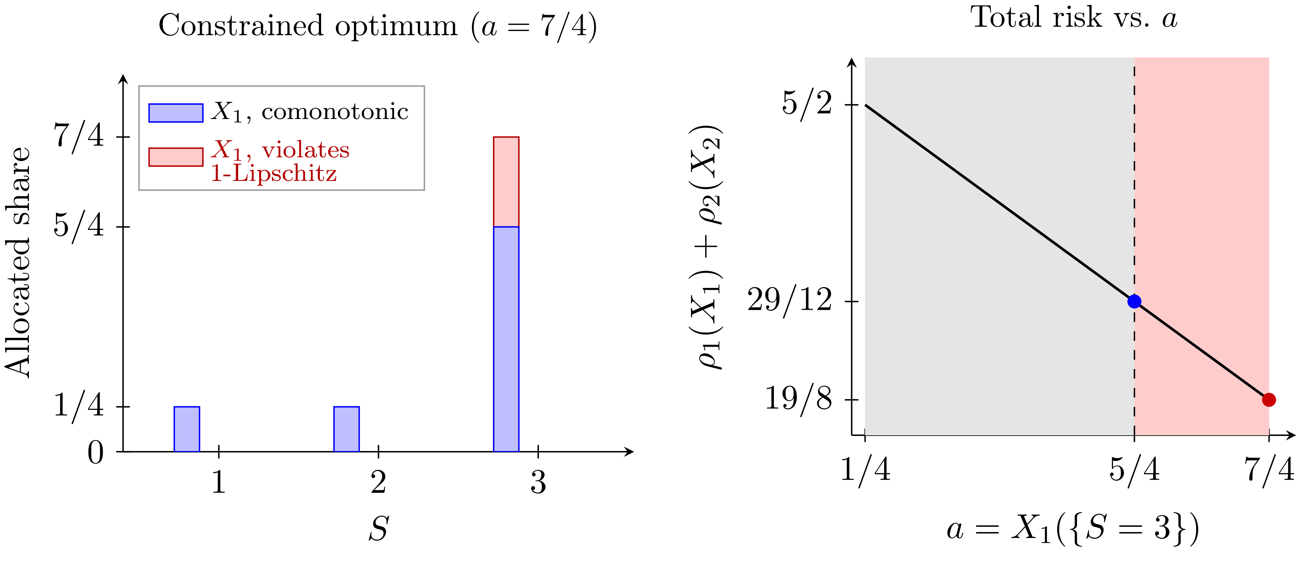
Example 2. Let S take the values 1, 2, 3 with probability $1/3$
each and write
$1/3$
each and write $X_2=S-X_1$
. The treaty fixes a deterministic retention on non-catastrophe states and a step-up cap on the catastrophe state. We model it as an aggregate-indexed treaty, that requires
$X_2=S-X_1$
. The treaty fixes a deterministic retention on non-catastrophe states and a step-up cap on the catastrophe state. We model it as an aggregate-indexed treaty, that requires $X_1$
to be
$X_1$
to be $\sigma(S)$
-measurable together with
$\sigma(S)$
-measurable together with $X_1=1/4$
on
$X_1=1/4$
on $\{S\le2\}$
and
$\{S\le2\}$
and $1/4\le X_1\le 7/4$
on
$1/4\le X_1\le 7/4$
on $\{S=3\}$
. The
$\{S=3\}$
. The $\sigma(S)$
-measurability restriction is part of the constraint: a treaty whose terms reference only the aggregate loss specifies the ceded amount as a function of S alone. We return below to what happens if this restriction is dropped. Under these constraints, every feasible allocation has the form
$\sigma(S)$
-measurability restriction is part of the constraint: a treaty whose terms reference only the aggregate loss specifies the ceded amount as a function of S alone. We return below to what happens if this restriction is dropped. Under these constraints, every feasible allocation has the form $X_1=\tfrac14\,{\unicode{x1D7D9}}_{\{S\le 2\}}+a\,{\unicode{x1D7D9}}_{\{S=3\}}$
and
$X_1=\tfrac14\,{\unicode{x1D7D9}}_{\{S\le 2\}}+a\,{\unicode{x1D7D9}}_{\{S=3\}}$
and $X_2=\tfrac34\,{\unicode{x1D7D9}}_{\{S=1\}}+\tfrac74\,{\unicode{x1D7D9}}_{\{S=2\}}+(3-a)\,{\unicode{x1D7D9}}_{\{S=3\}}$
for some
$X_2=\tfrac34\,{\unicode{x1D7D9}}_{\{S=1\}}+\tfrac74\,{\unicode{x1D7D9}}_{\{S=2\}}+(3-a)\,{\unicode{x1D7D9}}_{\{S=3\}}$
for some $a\in[1/4,7/4]$
. Since
$a\in[1/4,7/4]$
. Since $X_1$
is already nondecreasing in S, comonotonicity reduces to
$X_1$
is already nondecreasing in S, comonotonicity reduces to $X_2$
being nondecreasing in S, which requires
$X_2$
being nondecreasing in S, which requires $3-a\ge 7/4$
, that is,
$3-a\ge 7/4$
, that is, $a\le 5/4$
. We illustrate the feasible region of comonotonic allocations for this example in Figure 2.
$a\le 5/4$
. We illustrate the feasible region of comonotonic allocations for this example in Figure 2.
Take $\rho_1=\mathrm{ES}_{1/5}$
and
$\rho_1=\mathrm{ES}_{1/5}$
and $\rho_2=\mathrm{ES}_{1/3}$
. A direct computation shows that
$\rho_2=\mathrm{ES}_{1/3}$
. A direct computation shows that $\rho_1(X_1)+\rho_2(X_2)$
is strictly decreasing in a, so the constrained minimum is attained at
$\rho_1(X_1)+\rho_2(X_2)$
is strictly decreasing in a, so the constrained minimum is attained at $a^\star=7/4$
(value
$a^\star=7/4$
(value $19/8$
), while the comonotonic restriction
$19/8$
), while the comonotonic restriction $a\in[1/4,5/4]$
achieves only
$a\in[1/4,5/4]$
achieves only $29/12$
; the strict gap
$29/12$
; the strict gap $29/12-19/8=1/24\gt 0$
shows (2) fails. The comonotonic rearrangement of the optimizer (
$29/12-19/8=1/24\gt 0$
shows (2) fails. The comonotonic rearrangement of the optimizer ( $a=7/4$
) along S gives
$a=7/4$
) along S gives $\bar X_1=(1/4,3/4,5/4)$
, which violates the fixed-retention clause
$\bar X_1=(1/4,3/4,5/4)$
, which violates the fixed-retention clause $X_1=1/4$
on
$X_1=1/4$
on $\{S\le2\}$
, exhibiting the failure of componentwise convex-order solidity.
$\{S\le2\}$
, exhibiting the failure of componentwise convex-order solidity.
The mechanism behind Example 2 is that the constraint allows $X_1$
to jump by as much as
$X_1$
to jump by as much as $X_1(\{S=3\})-X_1(\{S=2\})=7/4-1/4=3/2$
when S moves from 2 to 3, while the aggregate loss itself increases by only
$X_1(\{S=3\})-X_1(\{S=2\})=7/4-1/4=3/2$
when S moves from 2 to 3, while the aggregate loss itself increases by only $S(3)-S(2)=1$
across the same step. In particular, the constraint specification fails the 1-Lipschitz comparison
$S(3)-S(2)=1$
across the same step. In particular, the constraint specification fails the 1-Lipschitz comparison $X_1(\{S=s'\})-X_1(\{S=s\})\le s'-s$
for
$X_1(\{S=s'\})-X_1(\{S=s\})\le s'-s$
for $s'\gt s$
: the admissible gap
$s'\gt s$
: the admissible gap $3/2$
strictly exceeds the aggregate-loss increment 1. The complementary allocation
$3/2$
strictly exceeds the aggregate-loss increment 1. The complementary allocation $X_2=S-X_1$
, therefore, decreases from the adverse layer to the catastrophe layer whenever agent 1 fully exploits the catastrophe capacity, which breaks the comonotonicity of
$X_2=S-X_1$
, therefore, decreases from the adverse layer to the catastrophe layer whenever agent 1 fully exploits the catastrophe capacity, which breaks the comonotonicity of $X_2$
with S. The unrestricted constrained optimizer uses the full catastrophe capacity. At
$X_2$
with S. The unrestricted constrained optimizer uses the full catastrophe capacity. At $S=3$
, raising
$S=3$
, raising $X_1$
by one unit increases
$X_1$
by one unit increases $\mathrm{ES}_{1/5}(X_1)$
by
$\mathrm{ES}_{1/5}(X_1)$
by $5/12$
but lowers
$5/12$
but lowers $\mathrm{ES}_{1/3}(X_2)$
by
$\mathrm{ES}_{1/3}(X_2)$
by $1/2$
, so shifting tail mass onto agent 1 lowers the sum
$1/2$
, so shifting tail mass onto agent 1 lowers the sum $\mathrm{ES}_{1/5}(X_1)+\mathrm{ES}_{1/3}(X_2)$
. The comonotonic class cannot reach this allocation: it can raise
$\mathrm{ES}_{1/5}(X_1)+\mathrm{ES}_{1/3}(X_2)$
. The comonotonic class cannot reach this allocation: it can raise $X_1$
on
$X_1$
on $\{S=3\}$
only to
$\{S=3\}$
only to $1+X_1$
on
$1+X_1$
on $\{S=2\}$
, that is, only to
$\{S=2\}$
, that is, only to $5/4$
, losing
$5/4$
, losing $1/2$
of tail capacity.
$1/2$
of tail capacity.
Mechanism in Example 2, with $X_1=1/4$
fixed on
$X_1=1/4$
fixed on $\{S\le2\}$
and
$\{S\le2\}$
and $X_1(\{S=3\})=a\in[1/4,7/4]$
free. Left: comonotonicity of
$X_1(\{S=3\})=a\in[1/4,7/4]$
free. Left: comonotonicity of $(X_1,X_2)$
with S is equivalent to the 1-Lipschitz comparison
$(X_1,X_2)$
with S is equivalent to the 1-Lipschitz comparison $X_1(\{S=3\})-$ $X_1(\{S=2\})\le S(\{S=3\})-S(\{S=2\})=1$
, that is, to the slope from
$X_1(\{S=2\})\le S(\{S=3\})-S(\{S=2\})=1$
, that is, to the slope from $(2,1/4)$
to (3, a) lying in [0, 1]. The dashed line is the slope-1 cone boundary; values on or below the cone (
$(2,1/4)$
to (3, a) lying in [0, 1]. The dashed line is the slope-1 cone boundary; values on or below the cone ( $a\in[1/4,5/4]$
, gray) are comonotonic, while
$a\in[1/4,5/4]$
, gray) are comonotonic, while $a\in(5/4,7/4]$
(red) remains constraint-feasible but breaks the monotonicity of
$a\in(5/4,7/4]$
(red) remains constraint-feasible but breaks the monotonicity of $X_2=S-X_1$
in S. Right: the constrained minimum
$X_2=S-X_1$
in S. Right: the constrained minimum $19/8$
at
$19/8$
at $a=7/4$
falls in the non-comonotonic region; the comonotonic minimum
$a=7/4$
falls in the non-comonotonic region; the comonotonic minimum $29/12$
at
$29/12$
at $a=5/4$
is strictly larger.
$a=5/4$
is strictly larger.
For a two-agent allocation $X_1=f(S)$
,
$X_1=f(S)$
, $X_2=S-f(S)$
with f a function of the aggregate loss, comonotonicity with S is equivalent to
$X_2=S-f(S)$
with f a function of the aggregate loss, comonotonicity with S is equivalent to $0\le f(t)-f(s)\le t-s$
, where
$0\le f(t)-f(s)\le t-s$
, where $s\lt t$
, the slope-one boundary of Example 2 stated for general f. When f is absolutely continuous, this reads
$s\lt t$
, the slope-one boundary of Example 2 stated for general f. When f is absolutely continuous, this reads $0\le f'\le 1$
. For an aggregate-indexed band
$0\le f'\le 1$
. For an aggregate-indexed band $\ell(S)\le X_1\le u(S)$
, one-Lipschitzness of an endpoint is not enough, because a feasible f can sit at the top of the band at one state and at the bottom at a higher state. In a pool of several agents the requirement is system-level rather than per-cap: individually one-Lipschitz capacities can jointly release more than one unit per unit increase in S, forcing some residual share to fall.
$\ell(S)\le X_1\le u(S)$
, one-Lipschitzness of an endpoint is not enough, because a feasible f can sit at the top of the band at one state and at the bottom at a higher state. In a pool of several agents the requirement is system-level rather than per-cap: individually one-Lipschitz capacities can jointly release more than one unit per unit increase in S, forcing some residual share to fall.
A convenient sufficient condition for aggregate-indexed bands is that, as s increases, the feasible coordinate ranges move upward together. Thus, the bands should not open in a way that lets one agent’s feasible share fall when S rises. For each agent, let
 \begin{equation*}\underline{k}_i(s)\,:\!=\,\max\left\{\ell_i(s),\ s-\sum_{j\ne i}u_j(s)\right\},\qquad\overline{k}_i(s)\,:\!=\,\min\left\{u_i(s),\ s-\sum_{j\ne i}\ell_j(s)\right\}. \end{equation*}
Here, $\underline{k}_i(s)$
and
$\underline{k}_i(s)$
and $\overline{k}_i(s)$
are the smallest and largest statewise feasible values of agent i at aggregate state s, respectively.
$\overline{k}_i(s)$
are the smallest and largest statewise feasible values of agent i at aggregate state s, respectively.
Proposition 1. Suppose that, for every $s\lt t$
in the support of S,
$s\lt t$
in the support of S, $\overline{k}_i(s)\le \underline{k}_i(t)$
for
$\overline{k}_i(s)\le \underline{k}_i(t)$
for $i=1,\ldots,n$
. Then the aggregate-indexed band constraint is componentwise convex-order-solid.
$i=1,\ldots,n$
. Then the aggregate-indexed band constraint is componentwise convex-order-solid.
Proof. Let $\boldsymbol{X}$
be feasible and set
$\boldsymbol{X}$
be feasible and set $\widetilde X_i\,:\!=\,\mathbb{E}[X_i\mid S]$
for
$\widetilde X_i\,:\!=\,\mathbb{E}[X_i\mid S]$
for $i=1,\ldots,n$
. For each state s in the support of S, write
$i=1,\ldots,n$
. For each state s in the support of S, write $\widetilde x(s)\,:\!=\,\mathbb{E}[\boldsymbol{X}\mid S=s]$
. Since the clearing equation and the interval bounds are convex, conditioning preserves them:
$\widetilde x(s)\,:\!=\,\mathbb{E}[\boldsymbol{X}\mid S=s]$
. Since the clearing equation and the interval bounds are convex, conditioning preserves them: $\sum_i\widetilde x_i(s)=s$
and
$\sum_i\widetilde x_i(s)=s$
and $\ell_i(s)\le \widetilde x_i(s)\le u_i(s)$
for every i. Thus,
$\ell_i(s)\le \widetilde x_i(s)\le u_i(s)$
for every i. Thus, $\widetilde{\boldsymbol{X}}$
is feasible and clears S. The ordering condition implies that, if
$\widetilde{\boldsymbol{X}}$
is feasible and clears S. The ordering condition implies that, if $s\lt t$
, then
$s\lt t$
, then $\widetilde x_i(s)\le \overline{k}_i(s)\le \underline{k}_i(t)\le \widetilde x_i(t)$
. Hence, each function
$\widetilde x_i(s)\le \overline{k}_i(s)\le \underline{k}_i(t)\le \widetilde x_i(t)$
. Hence, each function $f_i(s)\,:\!=\,\widetilde x_i(s)$
is nondecreasing, so
$f_i(s)\,:\!=\,\widetilde x_i(s)$
is nondecreasing, so $\widetilde{\boldsymbol{X}}$
is comonotonic with S. Finally, conditioning reduces risk in convex order:
$\widetilde{\boldsymbol{X}}$
is comonotonic with S. Finally, conditioning reduces risk in convex order: $\widetilde X_i=\mathbb{E}[X_i\mid S]\le_{\mathrm{cx}} X_i$
for
$\widetilde X_i=\mathbb{E}[X_i\mid S]\le_{\mathrm{cx}} X_i$
for $i=1,\ldots,n$
. This is the required convex-order solidity property.
$i=1,\ldots,n$
. This is the required convex-order solidity property.
In the two-agent case with a single band $\ell(S)\le X_1\le u(S)$
, the condition reduces to the two no-crossing inequalities
$\ell(S)\le X_1\le u(S)$
, the condition reduces to the two no-crossing inequalities $u(s)\le \ell(t)$
and
$u(s)\le \ell(t)$
and $u(t)-\ell(s)\le t-s$
for
$u(t)-\ell(s)\le t-s$
for $s\lt t$
. The first inequality prevents
$s\lt t$
. The first inequality prevents $X_1$
from falling as S rises. The second prevents
$X_1$
from falling as S rises. The second prevents $X_1$
from rising faster than S, which would force
$X_1$
from rising faster than S, which would force $X_2=S-X_1$
to fall. When the band collapses to
$X_2=S-X_1$
to fall. When the band collapses to $\ell=u=f$
, these reduce to the one-Lipschitz condition above, and Example 2 violates the upper-increment condition
$\ell=u=f$
, these reduce to the one-Lipschitz condition above, and Example 2 violates the upper-increment condition $u(t)-\ell(s)\le t-s$
. We will provide another example of a nonsolid aggregate-indexed band in Section 6.6, where the total capacity is released faster than the aggregate loss itself, and the comonotonic rearrangement of the optimizer violates the band constraint.
$u(t)-\ell(s)\le t-s$
. We will provide another example of a nonsolid aggregate-indexed band in Section 6.6, where the total capacity is released faster than the aggregate loss itself, and the comonotonic rearrangement of the optimizer violates the band constraint.
Thus $\sigma(S)$
-measurability and monotonicity of the caps in S are not sufficient for convex-order solidity. What matters is the no-crossing condition: as S rises, the feasible coordinate ranges must move upward together.
$\sigma(S)$
-measurability and monotonicity of the caps in S are not sufficient for convex-order solidity. What matters is the no-crossing condition: as S rises, the feasible coordinate ranges must move upward together.
4.3 Value-at-Risk ceilings
The Value-at-Risk is not convex-order-consistent: a degenerate random variable can have higher $\mathrm{VaR}_\alpha$
than a dispersed one with the same mean, so a VaR ceiling is not convex-order-solid. In Example 3, the initial endowments are comonotonic and satisfy a Solvency-II-type
$\mathrm{VaR}_\alpha$
than a dispersed one with the same mean, so a VaR ceiling is not convex-order-solid. In Example 3, the initial endowments are comonotonic and satisfy a Solvency-II-type $\mathrm{VaR}_{0.995}$
constraint, yet the constrained infimum is not attained within the comonotonic class and the comonotonic-restricted value is strictly larger than the unrestricted constrained value.
$\mathrm{VaR}_{0.995}$
constraint, yet the constrained infimum is not attained within the comonotonic class and the comonotonic-restricted value is strictly larger than the unrestricted constrained value.
Example 3. Let $(A_0,A_{1a},A_{1b},A_2)$
be disjoint events with
$(A_0,A_{1a},A_{1b},A_2)$
be disjoint events with $\mathbb{P}(A_0)=0.9925$
,
$\mathbb{P}(A_0)=0.9925$
, $\mathbb{P}(A_{1a})=\mathbb{P}(A_{1b})=\mathbb{P}(A_2)=0.0025$
, and set
$\mathbb{P}(A_{1a})=\mathbb{P}(A_{1b})=\mathbb{P}(A_2)=0.0025$
, and set $A_1\,:\!=\,A_{1a}\cup A_{1b}$
, so that
$A_1\,:\!=\,A_{1a}\cup A_{1b}$
, so that $\mathbb{P}(A_1)=0.005$
. Define the comonotonic endowments
$\mathbb{P}(A_1)=0.005$
. Define the comonotonic endowments $\zeta_1=\zeta_2={\unicode{x1D7D9}}_{A_1}+2\,{\unicode{x1D7D9}}_{A_2}$
so that
$\zeta_1=\zeta_2={\unicode{x1D7D9}}_{A_1}+2\,{\unicode{x1D7D9}}_{A_2}$
so that $S=2\,{\unicode{x1D7D9}}_{A_1}+4\,{\unicode{x1D7D9}}_{A_2}$
. Take
$S=2\,{\unicode{x1D7D9}}_{A_1}+4\,{\unicode{x1D7D9}}_{A_2}$
. Take $\rho_1=\mathrm{ES}_{0.99}$
,
$\rho_1=\mathrm{ES}_{0.99}$
, $\rho_2=\mathrm{ES}_{0.9925}$
, and
$\rho_2=\mathrm{ES}_{0.9925}$
, and $\mathbb{C}=\{X_i\ge0,\;\mathrm{VaR}_{0.995}(X_i)\le 1,\;i=1,2\}$
. Under autarky
$\mathbb{C}=\{X_i\ge0,\;\mathrm{VaR}_{0.995}(X_i)\le 1,\;i=1,2\}$
. Under autarky $\mathrm{VaR}_{0.995}(\zeta_i)=1$
, so the endowment allocation is comonotonic and feasible. Nonnegativity of each share
$\mathrm{VaR}_{0.995}(\zeta_i)=1$
, so the endowment allocation is comonotonic and feasible. Nonnegativity of each share $X_i$
is part of the constraint.
$X_i$
is part of the constraint.
One may show that the minimizers of $\rho_1(X_1)+\rho_2(X_2)$
over
$\rho_1(X_1)+\rho_2(X_2)$
over $\mathbb A_2(S)$
,
$\mathbb A_2(S)$
, $\mathbb A_2^{\mathbb{C}}(S)$
, and
$\mathbb A_2^{\mathbb{C}}(S)$
, and $\mathbb A_2^{\mathbb{C}}(S)\cap\mathbb A_2^{+}(S)$
are, respectively,
$\mathbb A_2^{\mathbb{C}}(S)\cap\mathbb A_2^{+}(S)$
are, respectively,
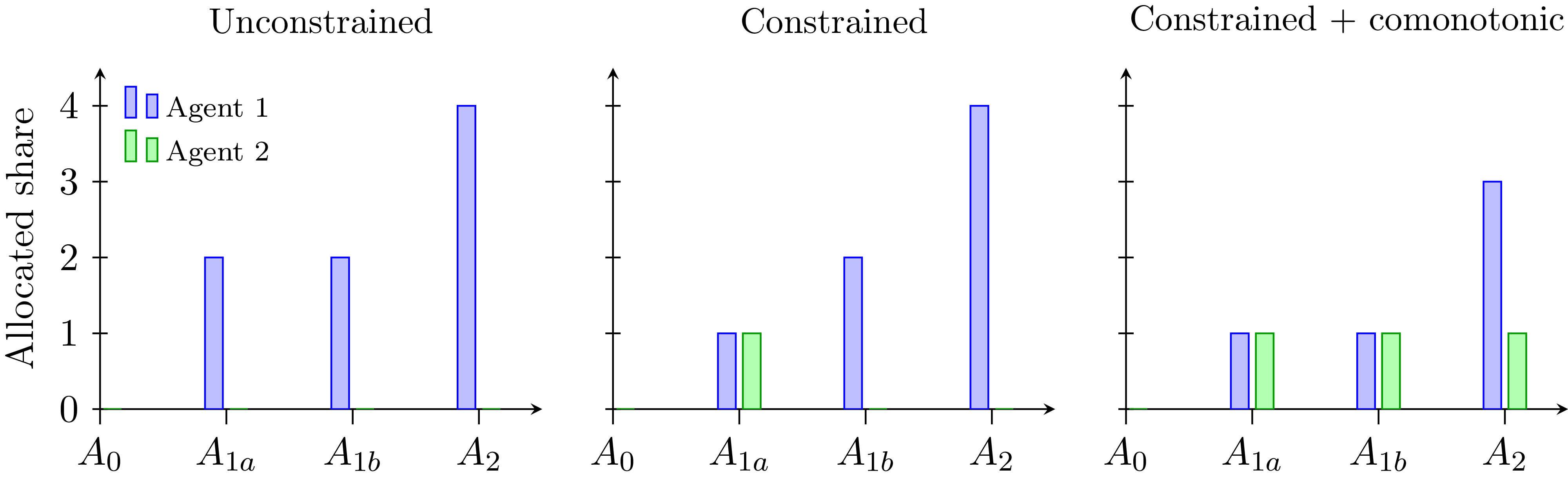
 \begin{equation*}\begin{aligned}(X_1,X_2)&=(S,\,0), & \sum_{i=1}^{2}\rho_i(X_i)&=2,\\[2pt](X_1,X_2)&=\left({\unicode{x1D7D9}}_{A_{1a}}+2\,{\unicode{x1D7D9}}_{A_{1b}}+4\,{\unicode{x1D7D9}}_{A_2},\ {\unicode{x1D7D9}}_{A_{1a}}\right), & \mathop{\kern.4em\square{_{\mathbb{C}}}}\limits_{i=1}^{2}\!\rho_i(S)&=25/12,\\[2pt](X_1,X_2)&=\left({\unicode{x1D7D9}}_{A_1}+3\,{\unicode{x1D7D9}}_{A_2},\ {\unicode{x1D7D9}}_{A_1}+{\unicode{x1D7D9}}_{A_2}\right), & \mathop{\kern.4em\boxplus{_{\mathbb{C}}}}\limits_{i=1}^{2}\!\rho_i(S)&=9/4.\end{aligned} \end{equation*}
Since $25/12\lt 9/4$
, the constrained comonotonic value strictly exceeds the constrained value, establishing non-comonotonicity of the constrained infimum. The mechanism is that a VaR ceiling permits a non-
$25/12\lt 9/4$
, the constrained comonotonic value strictly exceeds the constrained value, establishing non-comonotonicity of the constrained infimum. The mechanism is that a VaR ceiling permits a non- $\sigma(S)$
-measurable split of the intermediate loss layer:
$\sigma(S)$
-measurable split of the intermediate loss layer: $X_1^\star$
takes the value 1 on
$X_1^\star$
takes the value 1 on $A_{1a}$
and 2 on
$A_{1a}$
and 2 on $A_{1b}$
, even though
$A_{1b}$
, even though $S=2$
on both atoms. Comonotonicity forces each
$S=2$
on both atoms. Comonotonicity forces each $X_i$
to be constant on each level set of S, ruling out this selective assignment. A regulator who wants a tail-risk cap on each share can use ES in place of VaR. Among coherent, law-invariant risk measures that dominate
$X_i$
to be constant on each level set of S, ruling out this selective assignment. A regulator who wants a tail-risk cap on each share can use ES in place of VaR. Among coherent, law-invariant risk measures that dominate $\mathrm{VaR}_\alpha$
,
$\mathrm{VaR}_\alpha$
, $\mathrm{ES}_\alpha$
is the smallest, so an
$\mathrm{ES}_\alpha$
is the smallest, so an $\mathrm{ES}_\alpha$
cap at the same confidence level is the closest coherent tightening of the original
$\mathrm{ES}_\alpha$
cap at the same confidence level is the closest coherent tightening of the original $\mathrm{VaR}_\alpha$
cap. Coherence of ES makes its sublevel sets convex-order-solid, so Theorem 2 applies and the comonotonic reduction is restored. Figure 3 illustrates the optimal allocations under different allocation sets.
$\mathrm{VaR}_\alpha$
cap. Coherence of ES makes its sublevel sets convex-order-solid, so Theorem 2 applies and the comonotonic reduction is restored. Figure 3 illustrates the optimal allocations under different allocation sets.
The three minimizers in Example 3, shown on the four atoms $(\mathbb{P}(A_0)=0.9925$
,
$(\mathbb{P}(A_0)=0.9925$
, $\mathbb{P}(A_{1a})=\mathbb{P}(A_{1b})=\mathbb{P}(A_2)=0.0025)$
. The constrained optimum splits the level set
$\mathbb{P}(A_{1a})=\mathbb{P}(A_{1b})=\mathbb{P}(A_2)=0.0025)$
. The constrained optimum splits the level set $\{S=2\}=A_{1a}\cup A_{1b}$
asymmetrically. Since a comonotonic allocation must be constant on each level set of S, the comonotonic restriction forces equal shares on
$\{S=2\}=A_{1a}\cup A_{1b}$
asymmetrically. Since a comonotonic allocation must be constant on each level set of S, the comonotonic restriction forces equal shares on $A_{1a}$
and
$A_{1a}$
and $A_{1b}$
. This restriction yields a strictly larger total risk, namely
$A_{1b}$
. This restriction yields a strictly larger total risk, namely $9/4\gt 25/12$
.
$9/4\gt 25/12$
.
The splitting of the level set $\{S=2\}=A_{1a}\cup A_{1b}$
requires the probability space to be rich enough that this level set is not a single atom; on an atomless space, any level set of positive measure can be split, and the example applies whenever
$\{S=2\}=A_{1a}\cup A_{1b}$
requires the probability space to be rich enough that this level set is not a single atom; on an atomless space, any level set of positive measure can be split, and the example applies whenever $\mathbb{P}(S=2)\gt 0$
.
$\mathbb{P}(S=2)\gt 0$
.
Unconstrained problems with convex-order-consistent preferences admit comonotonic optima by the comonotonic improvement theorem, and distortion-riskmetric settings can exhibit comonotonic and counter-monotonic structures coexisting on different quantile segments (Lauzier et al., Reference Lauzier, Lin and Wang2026). The feasible allocation constructed above splits the level set $\{S=2\}$
across
$\{S=2\}$
across $A_{1a}$
and
$A_{1a}$
and $A_{1b}$
, so it is not
$A_{1b}$
, so it is not $\sigma(S)$
-measurable and cannot arise from any common quantile-segment reordering of the two shares. VaR constraints therefore admit feasible allocations that strictly improve on every comonotonic allocation and whose dependence structure is more intricate than a quantile-segment mixture.
$\sigma(S)$
-measurable and cannot arise from any common quantile-segment reordering of the two shares. VaR constraints therefore admit feasible allocations that strictly improve on every comonotonic allocation and whose dependence structure is more intricate than a quantile-segment mixture.
Solidity is sufficient for the comonotonic reduction but not necessary. The VaR constraint above destroys comonotonicity only under the heterogeneous Expected Shortfall objectives of that example. Under a common Expected Shortfall objective, the same feasible set admits a comonotonic optimum, the equal split $X_1=X_2=S/2$
. The same Value-at-Risk constraint can therefore destroy comonotonicity under one choice of preferences and preserve it under another. Solidity is therefore a broad, verifiable sufficient condition guaranteeing the reduction uniformly over convex-order-consistent preferences.
$X_1=X_2=S/2$
. The same Value-at-Risk constraint can therefore destroy comonotonicity under one choice of preferences and preserve it under another. Solidity is therefore a broad, verifiable sufficient condition guaranteeing the reduction uniformly over convex-order-consistent preferences.
One further inadmissible family involves lower bounds on convex-order-consistent functionals. Regulatory minimum capital or reserve charges that use a convex-order-monotone risk measure fit this pattern, including the Expected Shortfall charge on market risk under the Basel III FRTB and per-member reserve floors computed via variance-based or concave-distortion premium principles. Two-sided tolerance intervals around a target yield the same form $\varrho_i(X_i)\ge c_i$
with
$\varrho_i(X_i)\ge c_i$
with $\varrho_i$
convex-order-monotone. Because convex-order reduction decreases
$\varrho_i$
convex-order-monotone. Because convex-order reduction decreases $\varrho_i$
, such lower bounds are not convex-order-solid. The only admissible lower bound on a marginal-law functional is on the expectation, which convex order preserves exactly.
$\varrho_i$
, such lower bounds are not convex-order-solid. The only admissible lower bound on a marginal-law functional is on the expectation, which convex order preserves exactly.
The examples above separate three failure mechanisms. In Example 1, feasibility uses information beyond the aggregate loss: the deductible is a function of the agent’s idiosyncratic state, so the constraint is not $\sigma(S)$
-measurable. In Example 2, the aggregate capacity is released too quickly: once the least risk-averse agent is allowed to take a much larger share, clearing forces the remaining share to fall as the aggregate loss increases; thus, the solidity fails due to aggregate pathwise constraints. In Example 3, feasibility is marginal, since the VaR ceiling depends only on the law of the share. The failure comes from the lack of convex-order solidity of VaR sublevel sets. These examples show that admissibility depends on stability under componentwise convex-order reductions.
$\sigma(S)$
-measurable. In Example 2, the aggregate capacity is released too quickly: once the least risk-averse agent is allowed to take a much larger share, clearing forces the remaining share to fall as the aggregate loss increases; thus, the solidity fails due to aggregate pathwise constraints. In Example 3, feasibility is marginal, since the VaR ceiling depends only on the law of the share. The failure comes from the lack of convex-order solidity of VaR sublevel sets. These examples show that admissibility depends on stability under componentwise convex-order reductions.
5 Constraint families admitting comonotonic optima
This section gathers the constraint families most relevant to risk management and regulation that generate convex-order-solid feasible sets and therefore admit the reduction of Theorem 2. We collect four marginal constraint families whose induced feasible sets are componentwise convex-order-solid in Theorem 3. Convex piecewise-linear funding-cost adjustments folded into the objective are handled separately at the end of this section.
Before turning to concrete families, we record a one-dimensional version of solidity that we use to verify each family componentwise.
Definition 4 (Marginally convex-order-solid). A set $\mathfrak{C}\subseteq L^1$
is marginally convex-order-solid if
$\mathfrak{C}\subseteq L^1$
is marginally convex-order-solid if $Z\in\mathfrak{C}$
and
$Z\in\mathfrak{C}$
and $W\le_{\mathrm{cx}} Z$
imply
$W\le_{\mathrm{cx}} Z$
imply $W\in\mathfrak{C}$
.
$W\in\mathfrak{C}$
.
If each component constraint $X_i\in\mathfrak{C}_i$
is marginally convex-order-solid, then the feasible set
$X_i\in\mathfrak{C}_i$
is marginally convex-order-solid, then the feasible set $\{\boldsymbol{X}\in\mathbb{A}_n(S)\,:\,X_i\in\mathfrak{C}_i\ \text{for every }i\}$
is componentwise convex-order-solid in the sense of Definition 3. This is the mechanism through which Theorem 3 combines its four items; intersections close under both marginal and componentwise solidity, as established in Section 3.1.
$\{\boldsymbol{X}\in\mathbb{A}_n(S)\,:\,X_i\in\mathfrak{C}_i\ \text{for every }i\}$
is componentwise convex-order-solid in the sense of Definition 3. This is the mechanism through which Theorem 3 combines its four items; intersections close under both marginal and componentwise solidity, as established in Section 3.1.
Theorem 3 (Solid constraint families). Each of the following constraint sets is marginally convex-order-solid. Consequently, if for each $i \in [n]$
, the admissible marginal set
$i \in [n]$
, the admissible marginal set $\mathfrak{C}_i$
is any intersection of sets of the form (a)–(d), then the induced feasible set is componentwise convex-order-solid.
$\mathfrak{C}_i$
is any intersection of sets of the form (a)–(d), then the induced feasible set is componentwise convex-order-solid.
-
(a) Deterministic support bounds
$\{Z\in L^1\,:\, \ell\le Z\le u\ \text{a.s.}\}$
with
$\ell\in[-\infty,+\infty)$
,
$u\in(-\infty,+\infty]$
,
$\ell\le u$
. -
(b) Linear expectation constraints
$\{\mathbb{E}[Z]\le c\}$
,
$\{\mathbb{E}[Z]=c\}$
,
$\{\mathbb{E}[Z]\ge c\}$
. -
(c) Orlicz-type bounds
$\{\mathbb{E}[\varphi(Z)]\le c\}$
for convex
$\varphi\,:\,\mathbb{R}\to\mathbb{R}$
bounded below, including
$L^p$
-norm and entropic bounds; variance bounds
$\{\mathrm{Var}(Z)\le v\}$
follow from
$\varphi(x)=x^2$
together with preservation of the mean. -
(d) Risk-measure ceilings
$\{\varrho(Z)\le c\}$
for any convex-order-consistent
$\varrho\,:\,L^1\to\mathbb{R}\cup\{+\infty\}$
,
$c\in\mathbb{R}$
.







Proof. We verify that each family is marginally convex-order-solid. Since marginal convex-order solidity is preserved under intersections, the componentwise solidity of the induced feasible set follows immediately. In each case, we fix $Z\in\mathfrak{C}$
and
$Z\in\mathfrak{C}$
and $W\le_{\mathrm{cx}} Z$
and check that
$W\le_{\mathrm{cx}} Z$
and check that $W\in\mathfrak{C}$
.
$W\in\mathfrak{C}$
.
For item (a), suppose first that $u\lt +\infty$
and consider the convex hinge
$u\lt +\infty$
and consider the convex hinge $\phi_u(x)=(x-u)^+$
. Because
$\phi_u(x)=(x-u)^+$
. Because $Z\le u$
almost surely, one has
$Z\le u$
almost surely, one has $\phi_u(Z)=0$
a.s., so
$\phi_u(Z)=0$
a.s., so $\mathbb{E}[\phi_u(Z)]=0$
. Definition 2 applied to
$\mathbb{E}[\phi_u(Z)]=0$
. Definition 2 applied to $\phi_u$
then yields
$\phi_u$
then yields $\mathbb{E}[\phi_u(W)]\le 0$
, and since
$\mathbb{E}[\phi_u(W)]\le 0$
, and since $\phi_u\ge 0$
this forces
$\phi_u\ge 0$
this forces $\phi_u(W)=0$
a.s., that is,
$\phi_u(W)=0$
a.s., that is, $W\le u$
a.s. The lower bound
$W\le u$
a.s. The lower bound $W\ge\ell$
a.s. follows by the same argument with
$W\ge\ell$
a.s. follows by the same argument with $\phi_\ell(x)=(\ell-x)^+$
whenever
$\phi_\ell(x)=(\ell-x)^+$
whenever $\ell\gt -\infty$
. If
$\ell\gt -\infty$
. If $u=+\infty$
or
$u=+\infty$
or $\ell=-\infty$
, the corresponding inequality is vacuous.
$\ell=-\infty$
, the corresponding inequality is vacuous.
For item (b), both $x\mapsto x$
and
$x\mapsto x$
and $x\mapsto -x$
are convex, so Definition 2 yields
$x\mapsto -x$
are convex, so Definition 2 yields $\mathbb{E}[W]\le\mathbb{E}[Z]$
and
$\mathbb{E}[W]\le\mathbb{E}[Z]$
and $-\mathbb{E}[W]\le-\mathbb{E}[Z]$
, hence
$-\mathbb{E}[W]\le-\mathbb{E}[Z]$
, hence $\mathbb{E}[W]=\mathbb{E}[Z]$
. The three sets
$\mathbb{E}[W]=\mathbb{E}[Z]$
. The three sets $\{\mathbb{E}[Z]\le c\}$
,
$\{\mathbb{E}[Z]\le c\}$
, $\{\mathbb{E}[Z]=c\}$
and
$\{\mathbb{E}[Z]=c\}$
and $\{\mathbb{E}[Z]\ge c\}$
are therefore each preserved under
$\{\mathbb{E}[Z]\ge c\}$
are therefore each preserved under $\le_{\mathrm{cx}}$
.
$\le_{\mathrm{cx}}$
.
For item (c), the test function $\varphi$
is convex by hypothesis, so Definition 2 gives
$\varphi$
is convex by hypothesis, so Definition 2 gives $\mathbb{E}[\varphi(W)]\le\mathbb{E}[\varphi(Z)]\le c$
; the boundedness below of
$\mathbb{E}[\varphi(W)]\le\mathbb{E}[\varphi(Z)]\le c$
; the boundedness below of $\varphi$
ensures that the extended expectations are well defined. The variance bound follows by taking
$\varphi$
ensures that the extended expectations are well defined. The variance bound follows by taking $\varphi(x)=x^2$
: combining
$\varphi(x)=x^2$
: combining $\mathbb{E}[W^2]\le\mathbb{E}[Z^2]$
with
$\mathbb{E}[W^2]\le\mathbb{E}[Z^2]$
with $\mathbb{E}[W]=\mathbb{E}[Z]$
from item (b) gives
$\mathbb{E}[W]=\mathbb{E}[Z]$
from item (b) gives $\mathrm{Var}(W)\le\mathrm{Var}(Z)\le v$
.
$\mathrm{Var}(W)\le\mathrm{Var}(Z)\le v$
.
For item (d), convex-order consistency of $\varrho$
is exactly the implication
$\varrho$
is exactly the implication $W\le_{\mathrm{cx}} Z\Rightarrow\varrho(W)\le\varrho(Z)$
, so
$W\le_{\mathrm{cx}} Z\Rightarrow\varrho(W)\le\varrho(Z)$
, so $\varrho(W)\le\varrho(Z)\le c$
directly.
$\varrho(W)\le\varrho(Z)\le c$
directly.
Item (d) applies to every law-invariant coherent risk measure and to every distortion risk measure with a concave distortion, including Expected Shortfall, spectral measures, Wang transforms with concave generator, and proportional hazard transforms; see Wang and Young (Reference Wang and Young1998) and Dhaene et al. (Reference Dhaene, Denuit, Goovaerts, Kaas and Vyncke2002) for the convex-order properties of distortion risk measures. Expected Shortfall ceilings $\mathrm{ES}_{\alpha_i}(X_i)\le R_i$
, such as those used in the Basel FRTB framework and the Swiss Solvency Test, therefore generate convex-order-solid feasibility sets, while VaR-based regimes such as the Solvency II standard capital requirement fall under the caveat in Section 4.3. Heterogeneity of
$\mathrm{ES}_{\alpha_i}(X_i)\le R_i$
, such as those used in the Basel FRTB framework and the Swiss Solvency Test, therefore generate convex-order-solid feasibility sets, while VaR-based regimes such as the Solvency II standard capital requirement fall under the caveat in Section 4.3. Heterogeneity of $\alpha_i$
across firms does not break solidity.
$\alpha_i$
across firms does not break solidity.
Corollary 1 (Capacity caps). For deterministic constants $K_i\in[0,+\infty]$
, the feasibility set
$K_i\in[0,+\infty]$
, the feasibility set $\{\boldsymbol{X}\in\mathbb{A}_n(S)\,:\, 0\le X_i\le K_i\ \text{a.s. for every } i\}$
is componentwise convex-order-solid, so Theorem 2 applies under the standing hypotheses whenever this set is nonempty.
$\{\boldsymbol{X}\in\mathbb{A}_n(S)\,:\, 0\le X_i\le K_i\ \text{a.s. for every } i\}$
is componentwise convex-order-solid, so Theorem 2 applies under the standing hypotheses whenever this set is nonempty.
Corollary 1 covers limited-liability clauses, per-member capacity limits in reinsurance pools, layer widths in excess-of-loss reinsurance programmes, and public–private pool structures with heterogeneous governmental backstop caps. The analysis of inadmissible constraints in Section 4 shows why the cap $K_i$
must be a deterministic constant rather than a function of S with over-unit slope and rules out caps depending on state variables outside
$K_i$
must be a deterministic constant rather than a function of S with over-unit slope and rules out caps depending on state variables outside $\sigma(S)$
.
$\sigma(S)$
.
Aggregate-indexed pathwise bounds $\ell(S)\le X_i\le u(S)$
with nondecreasing
$\ell(S)\le X_i\le u(S)$
with nondecreasing $\ell,u$
are not automatically admissible: Example 2 shows that monotonicity alone does not prevent the comonotonic rearrangement from violating the envelope. Such caps should be treated as potentially inadmissible unless a separate solidity argument is supplied.
$\ell,u$
are not automatically admissible: Example 2 shows that monotonicity alone does not prevent the comonotonic rearrangement from violating the envelope. Such caps should be treated as potentially inadmissible unless a separate solidity argument is supplied.
Premium budgets $\mathbb{E}[X_i]\le P_i$
and actuarial-fairness constraints
$\mathbb{E}[X_i]\le P_i$
and actuarial-fairness constraints $\mathbb{E}[X_i]=\mathbb{E}[\zeta_i]$
, which equate each agent’s expected post-allocation loss with its expected initial loss, are admissible by item (b); equality and lower-bound forms are admissible as well, a special feature of the linearity of
$\mathbb{E}[X_i]=\mathbb{E}[\zeta_i]$
, which equate each agent’s expected post-allocation loss with its expected initial loss, are admissible by item (b); equality and lower-bound forms are admissible as well, a special feature of the linearity of $\mathbb{E}$
.
$\mathbb{E}$
.
Each agent’s preferences may combine a baseline risk measure with a convex loading of the post-allocation loss without disturbing solidity of the feasible set. In tiered-capital or cost-of-funds models, agent i’s objective takes the form $\rho_i(X_i)+\mathbb{E}[\varphi_i(X_i)]$
, where
$\rho_i(X_i)+\mathbb{E}[\varphi_i(X_i)]$
, where $\varphi_i\,:\,\mathbb{R}\to\mathbb{R}$
is convex, nondecreasing, piecewise linear, and bounded below (so that
$\varphi_i\,:\,\mathbb{R}\to\mathbb{R}$
is convex, nondecreasing, piecewise linear, and bounded below (so that $\mathbb{E}[\varphi_i(X_i)]$
is an extended expectation with integrable negative part, taking values in
$\mathbb{E}[\varphi_i(X_i)]$
is an extended expectation with integrable negative part, taking values in $\mathbb{R}\cup\{+\infty\}$
). A typical specification is
$\mathbb{R}\cup\{+\infty\}$
). A typical specification is $\varphi_i(x)=\alpha_i(x-R_i)^+ +(\beta_i-\alpha_i){(x-R_i-B_i)^+}$
, with
$\varphi_i(x)=\alpha_i(x-R_i)^+ +(\beta_i-\alpha_i){(x-R_i-B_i)^+}$
, with $R_i\in\mathbb{R}$
a retention threshold,
$R_i\in\mathbb{R}$
a retention threshold, $B_i\ge0$
a layer width, and
$B_i\ge0$
a layer width, and $0\le\alpha_i\le\beta_i$
so that the slopes are nonnegative and nondecreasing, encoding a reserve, collateral, and fire-sale ladder. The adjusted objective is convex-order-consistent: convex-order consistency of
$0\le\alpha_i\le\beta_i$
so that the slopes are nonnegative and nondecreasing, encoding a reserve, collateral, and fire-sale ladder. The adjusted objective is convex-order-consistent: convex-order consistency of $X\mapsto\mathbb{E}[\varphi_i(X)]$
follows by applying Definition 2 to the convex test function
$X\mapsto\mathbb{E}[\varphi_i(X)]$
follows by applying Definition 2 to the convex test function $\varphi_i$
, and summing with the convex-order-consistent
$\varphi_i$
, and summing with the convex-order-consistent $\rho_i$
preserves the property, so Theorem 2 applies directly on any convex-order-solid feasibility set.
$\rho_i$
preserves the property, so Theorem 2 applies directly on any convex-order-solid feasibility set.
6 Application: constrained mean-variance risk-sharing
We illustrate Theorem 2 on the mean-variance risk-sharing problem. The unconstrained mean-variance planner admits a well-known affine quota-share optimum. Under deterministic caps and floors, Theorem 3(a) (and Corollary 1 in the special case $L_i=0$
) licenses the comonotonic reduction, and the constrained optimum takes a truncated-affine form driven by a single statewise shadow price. Hard caps produce a piecewise-linear sharing rule with slopes determined by the active set of uncapped agents.
$L_i=0$
) licenses the comonotonic reduction, and the constrained optimum takes a truncated-affine form driven by a single statewise shadow price. Hard caps produce a piecewise-linear sharing rule with slopes determined by the active set of uncapped agents.
6.1 Unconstrained mean-variance sharing
Fix risk aversion parameters $\delta_1,\dots,\delta_n\gt 0$
and assume
$\delta_1,\dots,\delta_n\gt 0$
and assume $S\in L^2$
throughout this section. Each agent i evaluates its share through the mean-variance risk measure
$S\in L^2$
throughout this section. Each agent i evaluates its share through the mean-variance risk measure
 \begin{equation}\rho_i(X)\ \,:\!=\,\ \mathbb{E}[X]+\delta_i\,\mathrm{Var}(X),\qquad X\in L^2.\end{equation}
The functional $\rho_i$
is law-invariant and convex-order-consistent: if
$\rho_i$
is law-invariant and convex-order-consistent: if $Y\le_{\mathrm{cx}} X$
with
$Y\le_{\mathrm{cx}} X$
with $X\in L^2$
, then Definition 2 applied with
$X\in L^2$
, then Definition 2 applied with $\varphi(x)=x^2$
gives
$\varphi(x)=x^2$
gives $\mathbb{E}[Y^2]\le\mathbb{E}[X^2]\lt \infty$
, so
$\mathbb{E}[Y^2]\le\mathbb{E}[X^2]\lt \infty$
, so $Y\in L^2$
, and combined with
$Y\in L^2$
, and combined with $\mathbb{E}[Y]=\mathbb{E}[X]$
this yields
$\mathbb{E}[Y]=\mathbb{E}[X]$
this yields $\mathrm{Var}(Y)\le\mathrm{Var}(X)$
and therefore
$\mathrm{Var}(Y)\le\mathrm{Var}(X)$
and therefore $\rho_i(Y)\le\rho_i(X)$
. Assumption 1 is in force on the domain
$\rho_i(Y)\le\rho_i(X)$
. Assumption 1 is in force on the domain $L^2$
.
$L^2$
.
The clearing condition forces $\sum_i\mathbb{E}[X_i]=\mathbb{E}[S]$
, so the unconstrained risk-sharing problem
$\sum_i\mathbb{E}[X_i]=\mathbb{E}[S]$
, so the unconstrained risk-sharing problem
 \begin{equation}\inf_{\boldsymbol{X}\in\mathbb{A}_n(S)\cap(L^2)^n}\sum_{i=1}^n\rho_i(X_i)\end{equation}
is equivalent, up to the additive constant $\mathbb{E}[S]$
, to the pure variance-minimization problem
$\mathbb{E}[S]$
, to the pure variance-minimization problem
 \begin{equation*}\inf_{\boldsymbol{X}\in\mathbb{A}_n(S)\cap(L^2)^n}\sum_{i=1}^n\delta_i\,\mathrm{Var}(X_i). \end{equation*}
The following proposition is the mean-variance instance of the proportional sharing rule for dilated risk measures, noted in Acciaio (Reference Acciaio2007), Remark 4.6; see Barrieu and El Karoui (Reference Barrieu and El Karoui2005), Theorem 3.9 for a proof and Bernard and Vanduffel (Reference Bernard and Vanduffel2025) for a related statement. We state it to fix the notation used in the constrained problem.
Proposition 2. The unconstrained mean-variance problem (5) admits the optimum
 \begin{equation}X_i^{\star}\ =\ \frac{\delta_i^{-1}}{\sum_{j=1}^n\delta_j^{-1}}\,S\,+\,\beta_i,\end{equation}
where $\beta_1,\dots,\beta_n\in\mathbb{R}$
with
$\beta_1,\dots,\beta_n\in\mathbb{R}$
with $\sum_i\beta_i=0$
; the optimizer is unique
$\sum_i\beta_i=0$
; the optimizer is unique $\mathbb{P}$
-a.s. up to cash transfers
$\mathbb{P}$
-a.s. up to cash transfers ${\beta}$
.
${\beta}$
.
6.2 Constrained mean-variance risk-sharing
Impose deterministic capacity bounds on each share:
 \begin{equation}L_i\ \le\ X_i\ \le\ U_i\qquad\text{a.s.,}\qquad i\in[n],\end{equation}
with $L_i\in[-\infty,+\infty)$
,
$L_i\in[-\infty,+\infty)$
, $U_i\in(-\infty,+\infty]$
,
$U_i\in(-\infty,+\infty]$
, $L_i\lt U_i$
, and
$L_i\lt U_i$
, and $\sum_iL_i\le S\le\sum_iU_i$
a.s. in the extended sense. Let
$\sum_iL_i\le S\le\sum_iU_i$
a.s. in the extended sense. Let
 \begin{equation*}\mathbb{A}_n^{\mathrm{cap}}(S)\ \,:\!=\,\ \left\{\boldsymbol{X}\in\mathbb{A}_n(S)\cap\left(L^2\right)^n:\ L_i\le X_i\le U_i\ \text{a.s.}\ \forall i\right\}. \end{equation*}
The constrained mean-variance problem is
 \begin{equation}\inf_{\boldsymbol{X}\in\mathbb{A}_n^{\mathrm{cap}}(S)}\sum_{i=1}^n\rho_i(X_i).\end{equation}
Applied componentwise, Theorem 3(a) shows that $\mathbb{A}_n^{\mathrm{cap}}(S)$
is componentwise convex-order-solid in the sense of Definition 3, and convex order preserves
$\mathbb{A}_n^{\mathrm{cap}}(S)$
is componentwise convex-order-solid in the sense of Definition 3, and convex order preserves $L^2$
membership, so the comonotonic improvement stays in
$L^2$
membership, so the comonotonic improvement stays in $(L^2)^n$
. Theorem 2 therefore yields the reduction
$(L^2)^n$
. Theorem 2 therefore yields the reduction
 \begin{equation*}\inf_{\boldsymbol{X}\in\mathbb{A}_n^{\mathrm{cap}}(S)}\sum_i\rho_i(X_i)\ =\ \inf_{\boldsymbol{X}\in\mathbb{A}_n^{\mathrm{cap}}(S)\cap\mathbb{A}_n^{+}(S)}\sum_i\rho_i(X_i), \end{equation*}
so we may restrict attention to comonotonic allocations of the form $X_i=f_i(S)$
with
$X_i=f_i(S)$
with $f_i\,:\,\mathbb{R}\to[L_i,U_i]$
nondecreasing and
$f_i\,:\,\mathbb{R}\to[L_i,U_i]$
nondecreasing and $\sum_if_i(s)=s$
for
$\sum_if_i(s)=s$
for $F_S$
-a.e. s. Let
$F_S$
-a.e. s. Let $\mathcal{S}\,:\!=\,\mathrm{supp}(F_S)$
denote the topological support of S, that is, the smallest closed set
$\mathcal{S}\,:\!=\,\mathrm{supp}(F_S)$
denote the topological support of S, that is, the smallest closed set $K\subseteq\mathbb{R}$
with
$K\subseteq\mathbb{R}$
with $\mathbb{P}(S\in K)=1$
. Since the optimum has the form
$\mathbb{P}(S\in K)=1$
. Since the optimum has the form $X_i^\star=f_i^\star(S)$
, the functions
$X_i^\star=f_i^\star(S)$
, the functions $f_i^\star$
are pinned down only on
$f_i^\star$
are pinned down only on $\mathcal{S}$
; statements below about the shape of
$\mathcal{S}$
; statements below about the shape of $s\mapsto f_i^\star(s)$
therefore refer to
$s\mapsto f_i^\star(s)$
therefore refer to $s\in\mathcal{S}$
and hold up to
$s\in\mathcal{S}$
and hold up to $F_S$
-null sets.
$F_S$
-null sets.
The following theorem identifies the form of the constrained optimum.
Theorem 4. Any solution $\boldsymbol{X}^{\star}$
to problem (8) has the form
$\boldsymbol{X}^{\star}$
to problem (8) has the form
 \begin{equation}X_i^{\star}\ =\ \Pi_i\!\left(c_i^{\star}+\delta_i^{-1}\,\eta^{\star}(S)\right)\quad\text{a.s.},\qquad\Pi_i(x)\ \,:\!=\,\ \min\!\left\{U_i,\ \max\!\left\{L_i,\ x\right\}\right\},\end{equation}
with $c_i^{\star}=\mathbb{E}[X_i^{\star}]$
and a nondecreasing
$c_i^{\star}=\mathbb{E}[X_i^{\star}]$
and a nondecreasing $\eta^{\star}\,:\,\mathcal{S}\to\mathbb{R}$
defined by the clearing condition
$\eta^{\star}\,:\,\mathcal{S}\to\mathbb{R}$
defined by the clearing condition
 \begin{equation*}\sum_i\Pi_i(c_i^{\star}+\delta_i^{-1}\eta^{\star}(s))=s. \end{equation*}
Furthermore, the map $s\mapsto f_i^{\star}(s)$
is affine with slope
$s\mapsto f_i^{\star}(s)$
is affine with slope
 \begin{equation}\frac{\mathrm{d} f_i^{\star}}{\mathrm{d} s}\ =\ \begin{cases}\displaystyle\frac{\delta_i^{-1}}{\sum_{j\in A}\delta_j^{-1}},&i\in A,\\[0.9em]0,&i\notin A\end{cases}\end{equation}
on any subinterval of $\mathcal{S}$
along which the active set
$\mathcal{S}$
along which the active set $A(s)\,:\!=\,\{i\in[n]\,:\,L_i\lt f_i^{\star}(s)\lt U_i\}$
is constant and equal to some nonempty
$A(s)\,:\!=\,\{i\in[n]\,:\,L_i\lt f_i^{\star}(s)\lt U_i\}$
is constant and equal to some nonempty $A\subseteq[n]$
.
$A\subseteq[n]$
.
Proof. By Theorem 3(a), applied componentwise, the constraint set $\mathbb{A}_n^{\mathrm{cap}}(S)$
is componentwise convex-order-solid in the sense of Definition 3. Theorem 2(i) then produces a feasible allocation comonotonic with S that componentwise dominates any given optimizer in convex order; since each
$\mathbb{A}_n^{\mathrm{cap}}(S)$
is componentwise convex-order-solid in the sense of Definition 3. Theorem 2(i) then produces a feasible allocation comonotonic with S that componentwise dominates any given optimizer in convex order; since each $\rho_i$
is consistent with convex order, this comonotonic allocation is itself optimal. Fix such an optimizer, write it as
$\rho_i$
is consistent with convex order, this comonotonic allocation is itself optimal. Fix such an optimizer, write it as $X_i^{\star}=f_i^{\star}(S)$
, and set
$X_i^{\star}=f_i^{\star}(S)$
, and set $c_i^{\star}\,:\!=\,\mathbb{E}[X_i^{\star}]$
. Since
$c_i^{\star}\,:\!=\,\mathbb{E}[X_i^{\star}]$
. Since $\sum_i\mathbb{E}[X_i]=\mathbb{E}[S]$
is fixed across
$\sum_i\mathbb{E}[X_i]=\mathbb{E}[S]$
is fixed across $\mathbb{A}_n^{\mathrm{cap}}(S)$
, the expectation part of the objective in (8) is constant, and only the variance term remains.
$\mathbb{A}_n^{\mathrm{cap}}(S)$
, the expectation part of the objective in (8) is constant, and only the variance term remains.
We first show that, for $F_S$
-a.e.
$F_S$
-a.e. $s\in\mathcal{S}$
, the vector
$s\in\mathcal{S}$
, the vector $f^{\star}(s)=(\,f_1^{\star}(s),\ldots,f_n^{\star}(s))$
solves the finite-dimensional statewise program
$f^{\star}(s)=(\,f_1^{\star}(s),\ldots,f_n^{\star}(s))$
solves the finite-dimensional statewise program $(Q_s)$
:
$(Q_s)$
:
 \begin{equation*}\min_{x\in\mathbb{R}^n}\sum_{i=1}^n\delta_i(x_i-c_i^{\star})^2\quad\text{s.t.}\quad\sum_{i=1}^n x_i=s,\ L_i\le x_i\le U_i. \end{equation*}
If this failed on a set of s-values with positive $F_S$
-mass, replacing
$F_S$
-mass, replacing $f^{\star}(s)$
on that set by the unique minimizer of
$f^{\star}(s)$
on that set by the unique minimizer of $(Q_s)$
would produce another feasible allocation
$(Q_s)$
would produce another feasible allocation $Y_i=g_i(S)\in\mathbb{A}_n^{\mathrm{cap}}(S)$
with
$Y_i=g_i(S)\in\mathbb{A}_n^{\mathrm{cap}}(S)$
with
 \begin{equation*}\sum_i\rho_i(Y_i)\ =\ \mathbb{E}[S]+\sum_i\delta_i\,\mathrm{Var}(Y_i)\ \le\ \mathbb{E}[S]+\sum_i\delta_i\,\mathbb{E}\left[\left(Y_i-c_i^{\star}\right)^2\right], \end{equation*}
whereas, using $\mathrm{Var}(X_i^{\star})=\mathbb{E}[(X_i^{\star}-c_i^{\star})^2]$
at the optimizer,
$\mathrm{Var}(X_i^{\star})=\mathbb{E}[(X_i^{\star}-c_i^{\star})^2]$
at the optimizer,
 \begin{equation*}\sum_i\rho_i(X_i^{\star})\ =\ \mathbb{E}[S]+\sum_i\delta_i\,\mathbb{E}\left[(X_i^{\star}-c_i^{\star})^2\right]. \end{equation*}
A statewise improvement on a positive-mass set makes the right-hand side strictly smaller, contradicting optimality of $\boldsymbol{X}^{\star}$
. Hence,
$\boldsymbol{X}^{\star}$
. Hence, $f^{\star}(s)$
solves
$f^{\star}(s)$
solves $(Q_s)$
for
$(Q_s)$
for $F_S$
-a.e. s.
$F_S$
-a.e. s.
It remains to solve $(Q_s)$
. This is a strictly convex quadratic program with affine and box constraints, so the KKT conditions are necessary and sufficient. With Lagrangian
$(Q_s)$
. This is a strictly convex quadratic program with affine and box constraints, so the KKT conditions are necessary and sufficient. With Lagrangian
 \begin{equation*}\mathcal{L}(x,\eta,\lambda,\mu)\ =\ \sum_{i=1}^n\delta_i\left(x_i-c_i^{\star}\right)^2-2\eta\!\left(\sum_{i=1}^n x_i-s\right)+\sum_{i=1}^n\lambda_i(L_i-x_i)+\sum_{i=1}^n\mu_i(x_i-U_i), \end{equation*}
the KKT system
 \begin{equation*}\sum_i x_i=s,\qquad L_i\le x_i\le U_i,\qquad 2\delta_i\left(x_i-c_i^{\star}\right)-2\eta-\lambda_i+\mu_i=0, \end{equation*}
 \begin{equation*}\lambda_i\left(x_i-L_i\right)=0,\qquad\mu_i\left(U_i-x_i\right)=0,\qquad\lambda_i,\mu_i\ge0, \end{equation*}
is equivalent to
 \begin{equation*}x_i\ =\ \Pi_i\!\left(c_i^{\star}+\delta_i^{-1}\eta\right),\qquad\Pi_i(x)=\min\{U_i,\max\{L_i,x\}\}. \end{equation*}
The clearing condition $\sum_i x_i=s$
then determines the multiplier
$\sum_i x_i=s$
then determines the multiplier $\eta^{\star}(s)$
through
$\eta^{\star}(s)$
through
 \begin{equation*}H(\eta^{\star}(s))\ =\ s,\qquad H(\eta)\ \,:\!=\,\ \sum_{i=1}^n\Pi_i\!\left(c_i^{\star}+\delta_i^{-1}\eta\right), \end{equation*}
and, since H is continuous and nondecreasing, a nondecreasing measurable selector $s\mapsto\eta^{\star}(s)$
exists. Combining,
$s\mapsto\eta^{\star}(s)$
exists. Combining,
 \begin{equation*}X_i^{\star}\ =\ \Pi_i\!\left(c_i^{\star}+\delta_i^{-1}\eta^{\star}(S)\right)\quad\text{a.s.,} \end{equation*}
which is the truncated-affine form (9).
Finally, on any subinterval of $\mathcal{S}$
along which the active set
$\mathcal{S}$
along which the active set $A=\{i\in[n]\,:\,L_i \lt f_i^{\star}(s) \lt U_i\}$
is constant, the inactive shares are fixed at their bounds and the clearing condition reduces to
$A=\{i\in[n]\,:\,L_i \lt f_i^{\star}(s) \lt U_i\}$
is constant, the inactive shares are fixed at their bounds and the clearing condition reduces to
 \begin{equation*}\sum_{i\in A}\left(c_i^{\star}+\delta_i^{-1}\eta^{\star}(s)\right)+\sum_{i\notin A}f_i^{\star}(s)\ =\ s, \end{equation*}
so $\eta^{\star}$
is affine in s on that interval. Differentiating yields
$\eta^{\star}$
is affine in s on that interval. Differentiating yields
 \begin{equation*}\frac{\mathrm{d} f_i^{\star}}{\mathrm{d} s}\ =\ \frac{\delta_i^{-1}}{\sum_{j\in A}\delta_j^{-1}}\ \text{for }i\in A,\qquad\frac{\mathrm{d} f_i^{\star}}{\mathrm{d} s}\ =\ 0\ \text{for }i\notin A, \end{equation*}
which is (10). When $L_i=-\infty$
and
$L_i=-\infty$
and $U_i=+\infty$
for every i,
$U_i=+\infty$
for every i, $\Pi_i$
is the identity and
$\Pi_i$
is the identity and $A=[n]$
, and the formula reduces to the unconstrained affine allocation (6).
$A=[n]$
, and the formula reduces to the unconstrained affine allocation (6).
Remark 2 (Existence and measurability of the shadow-price selector). Theorem 4 asserts that every comonotonic optimum has the truncated-affine form (9) through a nondecreasing measurable function $\eta^{\star}\,:\,\mathcal{S}\to\mathbb{R}$
of the aggregate loss. Two facts must hold for this claim to make sense: the statewise minimizer must be unique, and the multiplier that generates it must be choosable as a Borel function of s, even though the clearing condition does not pin
$\eta^{\star}\,:\,\mathcal{S}\to\mathbb{R}$
of the aggregate loss. Two facts must hold for this claim to make sense: the statewise minimizer must be unique, and the multiplier that generates it must be choosable as a Borel function of s, even though the clearing condition does not pin $\eta$
down uniquely when several
$\eta$
down uniquely when several $\eta$
-values give the same total. We record both here.
$\eta$
-values give the same total. We record both here.
For fixed $s\in\mathcal{S}$
, the statewise program
$s\in\mathcal{S}$
, the statewise program $(Q_s)$
in the proof of Theorem 4 has a strictly convex, coercive objective and a convex polyhedral feasible set, so it admits a unique minimizer
$(Q_s)$
in the proof of Theorem 4 has a strictly convex, coercive objective and a convex polyhedral feasible set, so it admits a unique minimizer $\hat x(s)$
. Dualizing the adding-up constraint yields
$\hat x(s)$
. Dualizing the adding-up constraint yields
 \begin{equation*}\hat x_i(s)\ =\ \Pi_i\!\left(c_i^{\star}+\delta_i^{-1}\,\eta(s)\right) \end{equation*}
for any $\eta(s)$
satisfying
$\eta(s)$
satisfying $H(\eta(s))=s$
, where
$H(\eta(s))=s$
, where $H(\eta)\,:\!=\,\sum_i\Pi_i(c_i^{\star}+\delta_i^{-1}\eta)$
is continuous and nondecreasing. The preimage
$H(\eta)\,:\!=\,\sum_i\Pi_i(c_i^{\star}+\delta_i^{-1}\eta)$
is continuous and nondecreasing. The preimage $H^{-1}(\{s\})$
is therefore a nonempty closed interval, possibly unbounded at boundary values of s, and
$H^{-1}(\{s\})$
is therefore a nonempty closed interval, possibly unbounded at boundary values of s, and $\hat x(s)$
is constant along it, so the nonuniqueness of
$\hat x(s)$
is constant along it, so the nonuniqueness of $\eta(s)$
does not affect the allocation on any flat region of H. Any nondecreasing measurable selector
$\eta(s)$
does not affect the allocation on any flat region of H. Any nondecreasing measurable selector $s\mapsto\eta^{\star}(s)$
of the multivalued inverse of H therefore defines a finite, single-valued and measurable
$s\mapsto\eta^{\star}(s)$
of the multivalued inverse of H therefore defines a finite, single-valued and measurable $\eta^{\star}\,:\,\mathcal{S}\to\mathbb{R}$
, so
$\eta^{\star}\,:\,\mathcal{S}\to\mathbb{R}$
, so $\hat X_i\,:\!=\,\hat x_i(S)$
is a Borel allocation comonotonic with S of the form claimed by Theorem 4.
$\hat X_i\,:\!=\,\hat x_i(S)$
is a Borel allocation comonotonic with S of the form claimed by Theorem 4.
The shadow price $\eta^{\star}(S)$
determines each agent’s share. It is nondecreasing and fixed by the clearing condition. As the aggregate loss grows it rises, and each additional unit is shared among the agents still below their caps in proportion to their risk tolerances, so agent i in the active set A absorbs the fraction
$\eta^{\star}(S)$
determines each agent’s share. It is nondecreasing and fixed by the clearing condition. As the aggregate loss grows it rises, and each additional unit is shared among the agents still below their caps in proportion to their risk tolerances, so agent i in the active set A absorbs the fraction $\delta_i^{-1}/\sum_{j\in A}\delta_j^{-1}$
. When an agent reaches its cap, it stops absorbing further loss and drops out of A, and the remaining agents re-share each additional unit among themselves in the same proportion, renormalized over the smaller set. The optimum is a layered quota share:
$\delta_i^{-1}/\sum_{j\in A}\delta_j^{-1}$
. When an agent reaches its cap, it stops absorbing further loss and drops out of A, and the remaining agents re-share each additional unit among themselves in the same proportion, renormalized over the smaller set. The optimum is a layered quota share: $\eta^{\star}(S)$
is the marginal rate at which the pool absorbs one more unit of aggregate loss, each capacity limit is an exhaustion point, and the participants split each successive layer pro rata by risk tolerance over the set still active on it.
$\eta^{\star}(S)$
is the marginal rate at which the pool absorbs one more unit of aggregate loss, each capacity limit is an exhaustion point, and the participants split each successive layer pro rata by risk tolerance over the set still active on it.
As in the unconstrained problem, the optimum is unique only up to a deterministic balanced cash transfer. The caps confine the admissible transfers to a bounded set fixed by the bounds and the support of S, so the optimal value is determined and the transfer freedom is narrower than in the unconstrained case, where every balanced transfer is optimal (Corollary 2).
Although they solve a different problem, the constrained Pareto-optimal risk exchanges of Gerber (Reference Gerber1979) and Bühlmann and Jewell (Reference Bühlmann and Jewell1979) yield the same optimal allocations, since the two formulations reduce to the same KKT conditions. However, the risk exchange constraints from Bühlmann and Jewell (Reference Bühlmann and Jewell1979) impose limits on an agent’s share of the other agents’ losses, which are not necessarily convex-order-solid, so the comonotonic reduction does not apply to their problem for general risk measures.
6.3 Two-agent example
Consider $n=2$
agents with risk aversion parameters
$n=2$
agents with risk aversion parameters $\delta_1,\delta_2\gt 0$
. Agent 1 faces a hard upper cap
$\delta_1,\delta_2\gt 0$
. Agent 1 faces a hard upper cap $U_1=C\gt 0$
and a lower bound
$U_1=C\gt 0$
and a lower bound $L_1=0$
; agent 2 is uncapped in the sense that
$L_1=0$
; agent 2 is uncapped in the sense that $L_2=-\infty$
and
$L_2=-\infty$
and $U_2=+\infty$
. Assume
$U_2=+\infty$
. Assume $S\ge 0$
a.s. The feasible set is
$S\ge 0$
a.s. The feasible set is
 \begin{equation*}\mathbb{A}_2^{\mathrm{cap}}(S)\ =\ \left\{(X_1,X_2)\,:\, X_1+X_2=S,\ 0\le X_1\le C\right\}. \end{equation*}
Write $a\,:\!=\,\delta_1^{-1}/(\delta_1^{-1}+\delta_2^{-1})\in(0,1)$
for the unconstrained quota share of agent 1, and assume the cap binds on a nontrivial set of states, that is,
$a\,:\!=\,\delta_1^{-1}/(\delta_1^{-1}+\delta_2^{-1})\in(0,1)$
for the unconstrained quota share of agent 1, and assume the cap binds on a nontrivial set of states, that is, $\mathbb{P}(aS\gt C)\gt 0$
, equivalently
$\mathbb{P}(aS\gt C)\gt 0$
, equivalently $\mathrm{ess\,sup} S\gt C/a$
.
$\mathrm{ess\,sup} S\gt C/a$
.
Corollary 2. The constrained mean-variance optima in the two-agent pool above take the form
 \begin{equation}X_1^{\star}\ =\ \min\!\left\{C,\ \max\!\left\{0,\ aS+\beta^{\star}\right\}\right\},\qquad X_2^{\star}\ =\ S-X_1^{\star}\quad\text{a.s.,}\end{equation}
where $\beta^{\star}\in\mathbb{R}$
is any solution of the fixed-point condition
$\beta^{\star}\in\mathbb{R}$
is any solution of the fixed-point condition
 \begin{equation}\beta^{\star}\ =\ \mathbb{E}\!\left[\min\!\left\{C,\ \max\!\left\{0,\ aS+\beta^{\star}\right\}\right\}\right]-a\,\mathbb{E}[S].\end{equation}
The fixed-point Equation (12) admits at least one solution $\beta^{\star}\in\mathbb{R}$
, and any such
$\beta^{\star}\in\mathbb{R}$
, and any such $\beta^{\star}$
yields an optimum of the form (11); the solution set is a closed interval
$\beta^{\star}$
yields an optimum of the form (11); the solution set is a closed interval $[\beta_-,\beta_+]$
of deterministic balanced cash transfers.
$[\beta_-,\beta_+]$
of deterministic balanced cash transfers.
Proof. Agent 2 is uncapped, so $\Pi_2$
is the identity in Theorem 4. On the states where the active set equals
$\Pi_2$
is the identity in Theorem 4. On the states where the active set equals $\{1,2\}$
, the slope formula (10) gives
$\{1,2\}$
, the slope formula (10) gives $\mathrm{d} X_1^{\star}/\mathrm{d} s=a$
; on the cap regions
$\mathrm{d} X_1^{\star}/\mathrm{d} s=a$
; on the cap regions $X_1^{\star}$
is pinned at 0 or C. Continuity of
$X_1^{\star}$
is pinned at 0 or C. Continuity of $s\mapsto f_1^{\star}(s)$
forces
$s\mapsto f_1^{\star}(s)$
forces
 \begin{equation*}X_1^{\star}\ =\ \Pi(aS+\beta^{\star}),\qquad\Pi(y)\,:\!=\,\min\{C,\max\{0,y\}\}, \end{equation*}
for some $\beta^{\star}\in\mathbb{R}$
identified from the interior identity
$\beta^{\star}\in\mathbb{R}$
identified from the interior identity $X_1^{\star}=aS+\beta^{\star}$
as
$X_1^{\star}=aS+\beta^{\star}$
as $\beta^{\star}=c_1^{\star}-a\mathbb{E}[S]$
, using
$\beta^{\star}=c_1^{\star}-a\mathbb{E}[S]$
, using $c_1^{\star}+c_2^{\star}=\mathbb{E}[S]$
. Combining with
$c_1^{\star}+c_2^{\star}=\mathbb{E}[S]$
. Combining with $c_1^{\star}=\mathbb{E}[X_1^{\star}]=\mathbb{E}[\Pi(aS+\beta^{\star})]$
yields the fixed-point Equation (12). Existence of
$c_1^{\star}=\mathbb{E}[X_1^{\star}]=\mathbb{E}[\Pi(aS+\beta^{\star})]$
yields the fixed-point Equation (12). Existence of $\beta^{\star}$
follows from existence of the optimum.
$\beta^{\star}$
follows from existence of the optimum.
Let $h(\beta)\,:\!=\,\mathbb{E}[\Pi(aS+\beta)]$
. Since
$h(\beta)\,:\!=\,\mathbb{E}[\Pi(aS+\beta)]$
. Since $\Pi$
is nondecreasing and 1-Lipschitz, so is h, and
$\Pi$
is nondecreasing and 1-Lipschitz, so is h, and $h(\beta)-\beta-a\mathbb{E}[S]$
is continuous and nonincreasing, so the solution set of (12) is a closed interval
$h(\beta)-\beta-a\mathbb{E}[S]$
is continuous and nonincreasing, so the solution set of (12) is a closed interval $[\beta_-,\beta_+]$
.
$[\beta_-,\beta_+]$
.
The allocation (11) is the classical quota-share-with-limit rule up to a deterministic transfer. Below the attachment $s=(C-\beta^{\star})/a$
the two agents pool loss in proportion to their tolerances, and above the attachment the capped agent stops absorbing loss while the uncapped agent takes the full excess. When the lower boundary
$s=(C-\beta^{\star})/a$
the two agents pool loss in proportion to their tolerances, and above the attachment the capped agent stops absorbing loss while the uncapped agent takes the full excess. When the lower boundary $\{X_1^{\star}=0\}$
does not bind (for instance, whenever
$\{X_1^{\star}=0\}$
does not bind (for instance, whenever $\beta^{\star}\ge 0$
and
$\beta^{\star}\ge 0$
and $S\ge 0$
a.s.), the single breakpoint at
$S\ge 0$
a.s.), the single breakpoint at $s=(C-\beta^{\star})/a$
is the only slope change and corresponds to agent 1 transitioning from interior to upper cap; below it the slopes are
$s=(C-\beta^{\star})/a$
is the only slope change and corresponds to agent 1 transitioning from interior to upper cap; below it the slopes are $(a,1-a)$
, above it they are (0, 1). The formula reproduces the limited-quota-share treaty documented in the standard reinsurance reference (Albrecher et al., Reference Albrecher, Beirlant and Teugels2017), up to the transfer
$(a,1-a)$
, above it they are (0, 1). The formula reproduces the limited-quota-share treaty documented in the standard reinsurance reference (Albrecher et al., Reference Albrecher, Beirlant and Teugels2017), up to the transfer $\beta^{\star}$
that the paper’s convention usually absorbs into a premium. The comonotonic reduction in Theorem 2, instantiated by Theorem 3(a) componentwise, is what allows restricting to this shape in the first place.
$\beta^{\star}$
that the paper’s convention usually absorbs into a premium. The comonotonic reduction in Theorem 2, instantiated by Theorem 3(a) componentwise, is what allows restricting to this shape in the first place.
6.4 Four-agent illustration
We display a four-agent allocation with deterministic capacity caps to illustrate the successive-saturation pattern that Theorem 4 produces. The primitives are mean-variance preferences $\rho_i(X)=\mathbb{E}[X]+\delta_i\mathrm{Var}(X)$
with
$\rho_i(X)=\mathbb{E}[X]+\delta_i\mathrm{Var}(X)$
with $\boldsymbol{\delta}=(2,3,5,6)$
, unconstrained quota-share slopes
$\boldsymbol{\delta}=(2,3,5,6)$
, unconstrained quota-share slopes $\boldsymbol{a}=(5/12,5/18,1/6,5/36)$
from Proposition 2, and upper caps
$\boldsymbol{a}=(5/12,5/18,1/6,5/36)$
from Proposition 2, and upper caps $\boldsymbol{U}=(5,8,3,+\infty)$
with
$\boldsymbol{U}=(5,8,3,+\infty)$
with $L_i=-\infty$
. Figure 4 shows the zero-intercept representative of the unconstrained family clipped by the caps, that is,
$L_i=-\infty$
. Figure 4 shows the zero-intercept representative of the unconstrained family clipped by the caps, that is, $\widetilde X_i(s)$
starts from
$\widetilde X_i(s)$
starts from $a_is$
and saturates at
$a_is$
and saturates at $U_i$
as s grows, with successive breakpoints at
$U_i$
as s grows, with successive breakpoints at $s_1=12$
(agent 1 saturates),
$s_1=12$
(agent 1 saturates), $s_2=31/2$
(agent 3 saturates), and
$s_2=31/2$
(agent 3 saturates), and $s_3=20$
(agent 2 saturates); between breakpoints the remaining uncapped agents re-share with renormalized slopes. This is not the literal optimizer of Theorem 4, whose intercepts
$s_3=20$
(agent 2 saturates); between breakpoints the remaining uncapped agents re-share with renormalized slopes. This is not the literal optimizer of Theorem 4, whose intercepts $c_i^{\star}=\mathbb{E}[X_i^{\star}]$
are determined by fixed-point conditions analogous to (12); the same saturation pattern persists under the endogenous intercepts, with breakpoints shifted accordingly.
$c_i^{\star}=\mathbb{E}[X_i^{\star}]$
are determined by fixed-point conditions analogous to (12); the same saturation pattern persists under the endogenous intercepts, with breakpoints shifted accordingly.
Capped quota-share allocations $\widetilde{X}_i(s)$
with upper caps
$\widetilde{X}_i(s)$
with upper caps $\boldsymbol{U}=(5,8,3,+\infty)$
and zero intercepts. Dotted vertical lines mark the breakpoints at which agents 1, 3, and 2 successively saturate their caps.
$\boldsymbol{U}=(5,8,3,+\infty)$
and zero intercepts. Dotted vertical lines mark the breakpoints at which agents 1, 3, and 2 successively saturate their caps.

6.5 Two-agent Value-at-Risk ceilings
Mean-variance risk-sharing is a classical setting in which every agent is variance-averse and the unconstrained optimum is an affine comonotonic quota share. Even here, a VaR ceiling is enough to break comonotonicity: the failure of convex-order solidity for VaR (Section 4.3) translates directly into a non-comonotonic optimum under continuous losses. To illustrate, take two variance-averse agents with loss evaluations $\rho_i(X)=\mathbb{E}[X]+\delta_i\mathrm{Var}(X)$
and parameters
$\rho_i(X)=\mathbb{E}[X]+\delta_i\mathrm{Var}(X)$
and parameters $(\delta_1,\delta_2)=(0.01,1)$
, so that agent 1 is much less variance-averse than agent 2. Let
$(\delta_1,\delta_2)=(0.01,1)$
, so that agent 1 is much less variance-averse than agent 2. Let $\zeta_1,\zeta_2\stackrel{\mathrm{iid}}{\sim}\mathrm{Exp}(1)$
, so
$\zeta_1,\zeta_2\stackrel{\mathrm{iid}}{\sim}\mathrm{Exp}(1)$
, so $S=\zeta_1+\zeta_2$
is gamma-distributed with shape 2 and rate 1 and impose the constraint
$S=\zeta_1+\zeta_2$
is gamma-distributed with shape 2 and rate 1 and impose the constraint
 \begin{equation*}X_1+X_2=S,\qquad X_i\ge 0,\qquad \mathrm{VaR}_{0.95}(X_i)\le 3,\quad i=1,2, \end{equation*}
under which autarky is feasible.
Set $\lambda\,:\!=\,\delta_1/(\delta_1+\delta_2)=1/101$
, the mean-constraint center
$\lambda\,:\!=\,\delta_1/(\delta_1+\delta_2)=1/101$
, the mean-constraint center $m^\star\approx 0.6337$
,
$m^\star\approx 0.6337$
, $a\,:\!=\,m^\star/(1-\lambda)\approx 0.6400$
,
$a\,:\!=\,m^\star/(1-\lambda)\approx 0.6400$
, $r\,:\!=\,(3+m^\star)/(1-\lambda)\approx 3.6700$
, and
$r\,:\!=\,(3+m^\star)/(1-\lambda)\approx 3.6700$
, and $q\,:\!=\,\mathrm{VaR}_{0.95}(S)\approx 4.7439$
. The constrained optimum is
$q\,:\!=\,\mathrm{VaR}_{0.95}(S)\approx 4.7439$
. The constrained optimum is $X_2^\star=f(S)$
,
$X_2^\star=f(S)$
, $X_1^\star=S-f(S)$
, with
$X_1^\star=S-f(S)$
, with
 \begin{equation*}f(s)\ =\ \begin{cases}s, & 0\le s\le a,\\m^\star+\lambda s, & a\lt s\le r,\\s-3, & r\lt s\le q,\\m^\star+\lambda s, & s\gt q.\end{cases} \end{equation*}
Figure 5 illustrates the optimal allocation for this allocation set. The map f is discontinuous at q: $f(q-)=q-3\approx 1.74$
, while
$f(q-)=q-3\approx 1.74$
, while $f(q+)\approx 0.68$
, so agent 2’s allocation drops as S crosses q. The constrained objective value is
$f(q+)\approx 0.68$
, so agent 2’s allocation drops as S crosses q. The constrained objective value is $\rho_1(X_1^\star)+\rho_2(X_2^\star)\approx 2.0517$
, whereas restricting to comonotonic allocations gives
$\rho_1(X_1^\star)+\rho_2(X_2^\star)\approx 2.0517$
, whereas restricting to comonotonic allocations gives $\approx$ $2.0972$
, confirming that the constrained infimum is not attained within the comonotonic class. The unconstrained optimum attains
$2.0972$
, confirming that the constrained infimum is not attained within the comonotonic class. The unconstrained optimum attains $\approx$ $2.0198$
and autarky (feasible, since
$2.0198$
and autarky (feasible, since $\mathrm{VaR}_{0.95}(\zeta_i)=-\log\!(0.05)\lt 3$
) attains
$\mathrm{VaR}_{0.95}(\zeta_i)=-\log\!(0.05)\lt 3$
) attains $3.01$
, so the four objective values rank as
$3.01$
, so the four objective values rank as $2.0198\lt 2.0517\lt 2.0972\lt 3.01$
.
$2.0198\lt 2.0517\lt 2.0972\lt 3.01$
.
The four regimes describe how the bounds activate in turn. On [0, a] the nonnegativity floor $X_1\ge 0$
binds and agent 2 absorbs the entire loss. On (a, r] both agents are interior and share loss affinely at the unconstrained slopes
$X_1\ge 0$
binds and agent 2 absorbs the entire loss. On (a, r] both agents are interior and share loss affinely at the unconstrained slopes $(1-\lambda,\lambda)$
, with the less-variance-averse agent 1 taking the lion’s share of marginal loss. On (r, q], agent 1 is pinned at the Value-at-Risk ceiling
$(1-\lambda,\lambda)$
, with the less-variance-averse agent 1 taking the lion’s share of marginal loss. On (r, q], agent 1 is pinned at the Value-at-Risk ceiling $X_1=3$
, so agent 2 absorbs every additional unit of loss. At
$X_1=3$
, so agent 2 absorbs every additional unit of loss. At $s=q$
, the ceiling stops binding: since
$s=q$
, the ceiling stops binding: since $\mathrm{VaR}_{0.95}$
is insensitive to the upper 5% tail, the planner may transfer the accumulated cap excess back to the less-averse agent 1 on
$\mathrm{VaR}_{0.95}$
is insensitive to the upper 5% tail, the planner may transfer the accumulated cap excess back to the less-averse agent 1 on $\{S\gt q\}$
and does so to restore the affine proportional interior slopes.
$\{S\gt q\}$
and does so to restore the affine proportional interior slopes.
Constrained mean-variance allocation under the $\mathrm{VaR}_{0.95}$
ceiling. At q, agent 2’s allocation drops and agent 1’s jumps up by the same amount, so neither is comonotonic with S globally.
$\mathrm{VaR}_{0.95}$
ceiling. At q, agent 2’s allocation drops and agent 1’s jumps up by the same amount, so neither is comonotonic with S globally.

The constrained allocation behaves differently across the state space: within each of the four regimes, both $X_1^\star$
and
$X_1^\star$
and $X_2^\star$
are nondecreasing in S, so the pair is comonotonic locally, but across the jump at q the two allocations move in opposite directions, with
$X_2^\star$
are nondecreasing in S, so the pair is comonotonic locally, but across the jump at q the two allocations move in opposite directions, with $X_1^\star$
rising while
$X_1^\star$
rising while $X_2^\star$
falls, so pairs of states straddling q exhibit counter-monotonic behavior. Note that here
$X_2^\star$
falls, so pairs of states straddling q exhibit counter-monotonic behavior. Note that here $X_i^\star=f_i(S)$
is
$X_i^\star=f_i(S)$
is $\sigma(S)$
-measurable, in contrast with Example 3 where the optimum splits the level set
$\sigma(S)$
-measurable, in contrast with Example 3 where the optimum splits the level set $\{S=2\}$
across
$\{S=2\}$
across $A_{1a}$
and
$A_{1a}$
and $A_{1b}$
and so fails to be
$A_{1b}$
and so fails to be $\sigma(S)$
-measurable; the atomless exponential marginals here rule out that mechanism, and non-comonotonicity instead shows up as the coexistence of comonotonic pieces and counter-monotonic cross-jump pairs. Because
$\sigma(S)$
-measurable; the atomless exponential marginals here rule out that mechanism, and non-comonotonicity instead shows up as the coexistence of comonotonic pieces and counter-monotonic cross-jump pairs. Because $\mathrm{VaR}_{0.95}$
does not see the upper 5% tail, the planner can still shift loss back to the less-averse agent beyond q, producing a feasible allocation that strictly improves on every comonotonic one.
$\mathrm{VaR}_{0.95}$
does not see the upper 5% tail, the planner can still shift loss back to the less-averse agent beyond q, producing a feasible allocation that strictly improves on every comonotonic one.
6.6 Aggregate-indexed caps that grow too fast
If one places capacity limits that depend on the aggregate loss, the constraint may not be convex-order-solid, as discussed in Proposition 1, and the comonotonic reduction may fail. The following example keeps the preferences mean-variance and the constraints $\sigma(S)$
-measurable but violates the no-crossing condition in Proposition 1 since the aggregate capacity is released too quickly.
$\sigma(S)$
-measurable but violates the no-crossing condition in Proposition 1 since the aggregate capacity is released too quickly.
Let $S\sim\mathrm{Unif}[0, 5]$
and consider three agents with
$S\sim\mathrm{Unif}[0, 5]$
and consider three agents with $X_1+X_2+X_3=S$
and
$X_1+X_2+X_3=S$
and $X_i\ge0$
. Agents 2 and 3 have identical aggregate-indexed caps
$X_i\ge0$
. Agents 2 and 3 have identical aggregate-indexed caps
 \begin{equation*} 0\le X_2\le u_2(S),\qquad 0\le X_3\le u_3(S),\qquad u_2(s)=u_3(s)=u(s) = \frac34 \max\{s-1,0\}. \end{equation*}
Each marginal cap is nondecreasing and has slope at most $3/4$
. However, the combined allocation
$3/4$
. However, the combined allocation $X_2+X_3$
can grow at slope
$X_2+X_3$
can grow at slope $3/2$
once
$3/2$
once $s\gt 1$
. Clearing is therefore equivalent to
$s\gt 1$
. Clearing is therefore equivalent to
 \begin{equation*} 0\le X_2+X_3\le u_2(S)+u_3(S)=2u(S),\qquad\ell(S)\le X_1\le u_1(S),\qquad u_1(s)=s, \end{equation*}
where
 \begin{equation*} \ell(s)=\max\{0,s-2u(s)\}=\begin{cases}s, & 0\le s\le 1,\\\dfrac32-\dfrac{s}{2}, & 1\lt s\le 3,\\0, & 3\lt s\le 5.\end{cases} \end{equation*}
Although the explicit restriction on agent 1 is only nonnegativity, clearing induces the lower bound $\ell(s)$
because, once agents 2 and 3 can absorb at most
$\ell(s)$
because, once agents 2 and 3 can absorb at most $u_2(s)+u_3(s)$
, agent 1 must take at least the residual
$u_2(s)+u_3(s)$
, agent 1 must take at least the residual $s-u_2(s)-u_3(s)$
. Thus, the lower feasible boundary for agent 1 decreases on (1, 3) and then stays at zero; this is exactly the system-level failure of the no-crossing condition. Figure 6 illustrates the constraints for this example.
$s-u_2(s)-u_3(s)$
. Thus, the lower feasible boundary for agent 1 decreases on (1, 3) and then stays at zero; this is exactly the system-level failure of the no-crossing condition. Figure 6 illustrates the constraints for this example.
Aggregate-indexed caps in the mean-variance counterexample. Each of agents 2 and 3 has marginal capacity $u_2(s)=u_3(s)=u(s)$
, while the combined capacity
$u_2(s)=u_3(s)=u(s)$
, while the combined capacity $u_2(s)+u_3(s)$
can grow faster than the upper feasible boundary
$u_2(s)+u_3(s)$
can grow faster than the upper feasible boundary $u_1(s)=s$
for agent 1. Hence, the feasible lower boundary
$u_1(s)=s$
for agent 1. Hence, the feasible lower boundary $\ell(s)$
for agent 1 decreases after the attachment point and is zero once the combined cap can absorb the whole aggregate loss.
$\ell(s)$
for agent 1 decreases after the attachment point and is zero once the combined cap can absorb the whole aggregate loss.

We use mean-variance preferences with variance loadings $\delta_1=1$
and
$\delta_1=1$
and $\delta_2=\delta_3=\delta$
, where
$\delta_2=\delta_3=\delta$
, where $0\lt \delta\le1/4$
. Since the expectation terms add to
$0\lt \delta\le1/4$
. Since the expectation terms add to $\mathbb{E}[S]$
, the nonconstant part of the objective function is the weighted variance term. Set
$\mathbb{E}[S]$
, the nonconstant part of the objective function is the weighted variance term. Set $\lambda\,:\!=\,\delta/(2+\delta)$
,
$\lambda\,:\!=\,\delta/(2+\delta)$
, $r\,:\!=\,\sqrt{3/(1+2\lambda)}$
, and
$r\,:\!=\,\sqrt{3/(1+2\lambda)}$
, and $c\,:\!=\,(3-\sqrt{3(1+2\lambda)})/2$
. The constrained optimum is
$c\,:\!=\,(3-\sqrt{3(1+2\lambda)})/2$
. The constrained optimum is
 \begin{equation*} f_1^\star(s)=\begin{cases}s, & 0\le s\le 1,\\\dfrac32-\dfrac{s}{2}, & 1\lt s\le r,\\\lambda s+c, & r\lt s\le 5,\end{cases}\qquad f_2^\star(s)=f_3^\star(s)=\frac{s-f_1^\star(s)}{2}. \end{equation*}
On (1, r) the caps of agents 2 and 3 bind, so $(\,f_2^\star)'(s)+(\,f_3^\star)'(s)=3/2$
. Clearing therefore gives
$(\,f_2^\star)'(s)+(\,f_3^\star)'(s)=3/2$
. Clearing therefore gives $(\,f_1^\star)'(s)=-1/2$
, so the allocation is not comonotonic. Thus,
$(\,f_1^\star)'(s)=-1/2$
, so the allocation is not comonotonic. Thus, $f_1^\star(s)=3/2-s/2$
until it meets the branch
$f_1^\star(s)=3/2-s/2$
until it meets the branch $\lambda s+c$
at
$\lambda s+c$
at $s=r$
. For
$s=r$
. For $r\lt s\le5$
, no cap binds and the slopes revert to the unconstrained slopes:
$r\lt s\le5$
, no cap binds and the slopes revert to the unconstrained slopes: $\lambda$
for agent 1 and
$\lambda$
for agent 1 and $(1-\lambda)/2$
for each of agents 2 and 3. Only the intercept changes.
$(1-\lambda)/2$
for each of agents 2 and 3. Only the intercept changes.
For Figure 7, set $\delta=1/4$
. Let
$\delta=1/4$
. Let $f^u$
,
$f^u$
, $f^\star$
, and
$f^\star$
, and $f^c$
denote the unconstrained optimum, the constrained optimum, and the constrained comonotonic optimum, respectively. The best comonotonic allocation is
$f^c$
denote the unconstrained optimum, the constrained optimum, and the constrained comonotonic optimum, respectively. The best comonotonic allocation is
 \begin{equation*} f_1^c(s)=\begin{cases}s, & 0\le s\le 1,\\1, & 1\lt s\le 3,\\[1mm]\dfrac{s}{9}+\dfrac23, & 3\lt s\le 5,\end{cases}\qquad f_2^c(s)=f_3^c(s)=\begin{cases}0, & 0\le s\le 1,\\\dfrac{s-1}{2}, & 1\lt s\le 3,\\[2mm]\dfrac49s-\dfrac13, & 3\lt s\le 5.\end{cases} \end{equation*}
The inf-convolutions are approximately $0.2536$
for the unrestricted constrained allocation and
$0.2536$
for the unrestricted constrained allocation and $0.2648$
for the best comonotonic feasible allocation. Thus, the constrained mean-variance optimum is strictly better than every comonotonic feasible allocation, illustrating the failure of the comonotonic reduction when the no-crossing condition is violated.
$0.2648$
for the best comonotonic feasible allocation. Thus, the constrained mean-variance optimum is strictly better than every comonotonic feasible allocation, illustrating the failure of the comonotonic reduction when the no-crossing condition is violated.
Unconstrained, constrained, and comonotonic constrained allocations for $\delta=1/4$
. In the constrained optimum, agents 2 and 3 jointly release capacity faster than the aggregate loss grows, forcing agent 1’s allocation to decrease on (1, r).
$\delta=1/4$
. In the constrained optimum, agents 2 and 3 jointly release capacity faster than the aggregate loss grows, forcing agent 1’s allocation to decrease on (1, r).

Figure 7. Long description
Three line graphs depict allocation strategies for agents under different conditions. Panel A: Unconstrained optimum. The line graph shows allocation on the vertical axis and s on the horizontal axis. The blue line represents f1u(s), and the green dashed line represents f2u(s) and f3u(s). Both lines increase as s increases. Panel B: Constrained optimum. The line graph shows allocation on the vertical axis and s on the horizontal axis. The blue line represents f1*(s), and the green dashed line represents f2*(s) and f3*(s). The blue line initially increases, then decreases, and finally increases again, while the green dashed line consistently increases. Panel C: Optimal comonotonic plus constrained. The line graph shows allocation on the vertical axis and s on the horizontal axis. The blue line represents f1c(s), and the green dashed line represents f2c(s) and f3c(s). The blue line increases and then levels off, while the green dashed line consistently increases.
7 Conclusion
The classical unconstrained comonotonic reduction of Borch (Reference Borch1962), Landsberger and Meilijson (Reference Landsberger and Meilijson1994), and Ludkovski and Rüschendorf (Reference Ludkovski and Rüschendorf2008) makes optimal risk-sharing under convex-order-consistent preferences tractable when the feasible set is the full clearing simplex. We extend the reduction to constrained problems. Theorem 2 shows that the comonotonic improvement theorem survives whenever the feasible set is componentwise convex-order-solid, and Theorem 3 identifies the operational constraint families that qualify, together with their stability under finite intersection. Solidity serves as a practical diagnostic for whether a given constraint system is compatible with the comonotonic reduction. It is not necessary but sufficient, and it guarantees that the optimal allocation can be found by restricting to the comonotonic class.
Not every constraint is admissible. Sections 4.3 and 6.5 show that VaR ceilings, which Solvency II imposes on insurers, escape the reduction even when every agent is risk-averse. Section 6.6 shows that aggregate-indexed capacity caps can also fail when the combined capacity released to some agents grows faster than the aggregate loss itself. Risk aversion alone does not guarantee comonotonic optima: the optimal sharing rule can combine comonotonic and counter-monotonic regions over the state space, so the dependence structure of the allocation departs from what the unconstrained intuition suggests.
Acknowledgments
The authors thank the AE and the two reviewers for their careful reading of the paper and for helpful suggestions. CBW acknowledges financial support from the Natural Sciences and Engineering Research Council of Canada (RGPIN-2025-06879).
Competing interests
The authors declare none.
Use of artificial intelligence tools
The authors used ChatGPT and Claude during manuscript preparation. The tools were used to assist with language editing, readability improvements, and proof checking. All AI-assisted output was reviewed, verified, and edited by the authors, who take full responsibility for the manuscript.
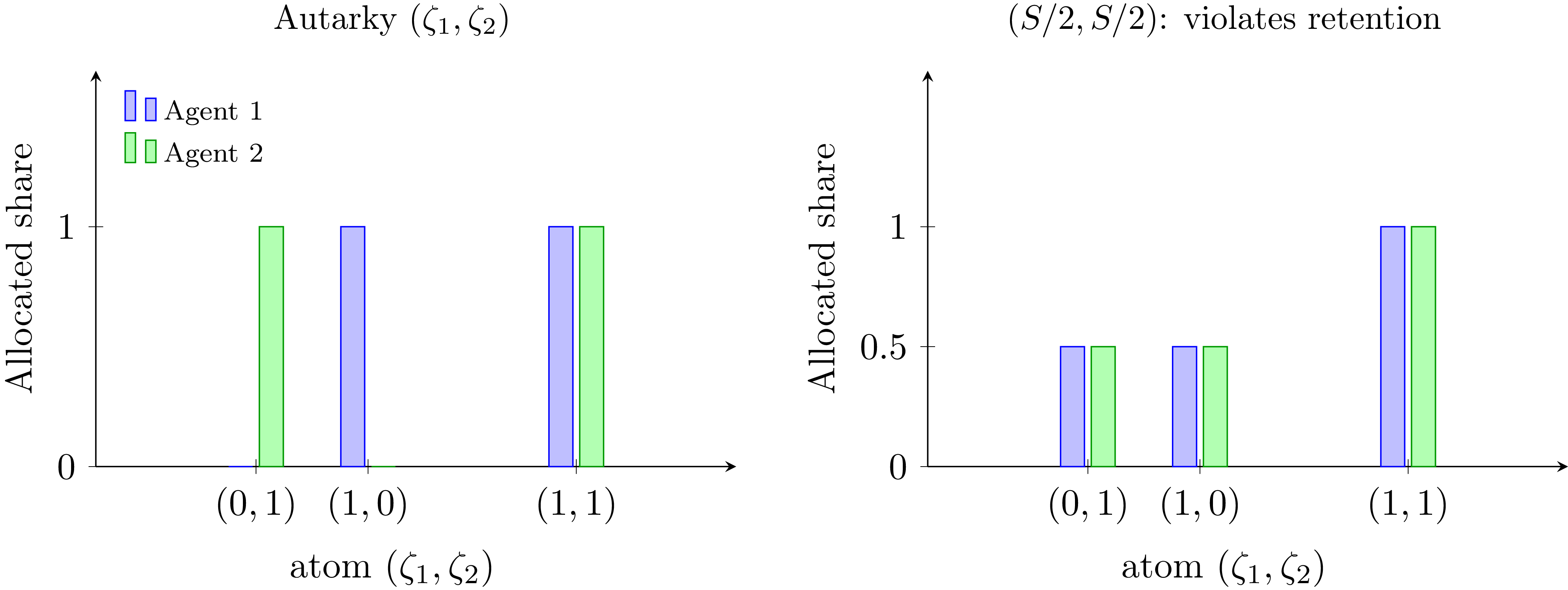
 (ζ1,ζ2)
 σ(S)
σ(S) X1
X1 {S=1}
{S=1} (S/2,S/2)
 σ(S)
σ(S) Xi=0
Xi=0 {ζi=0}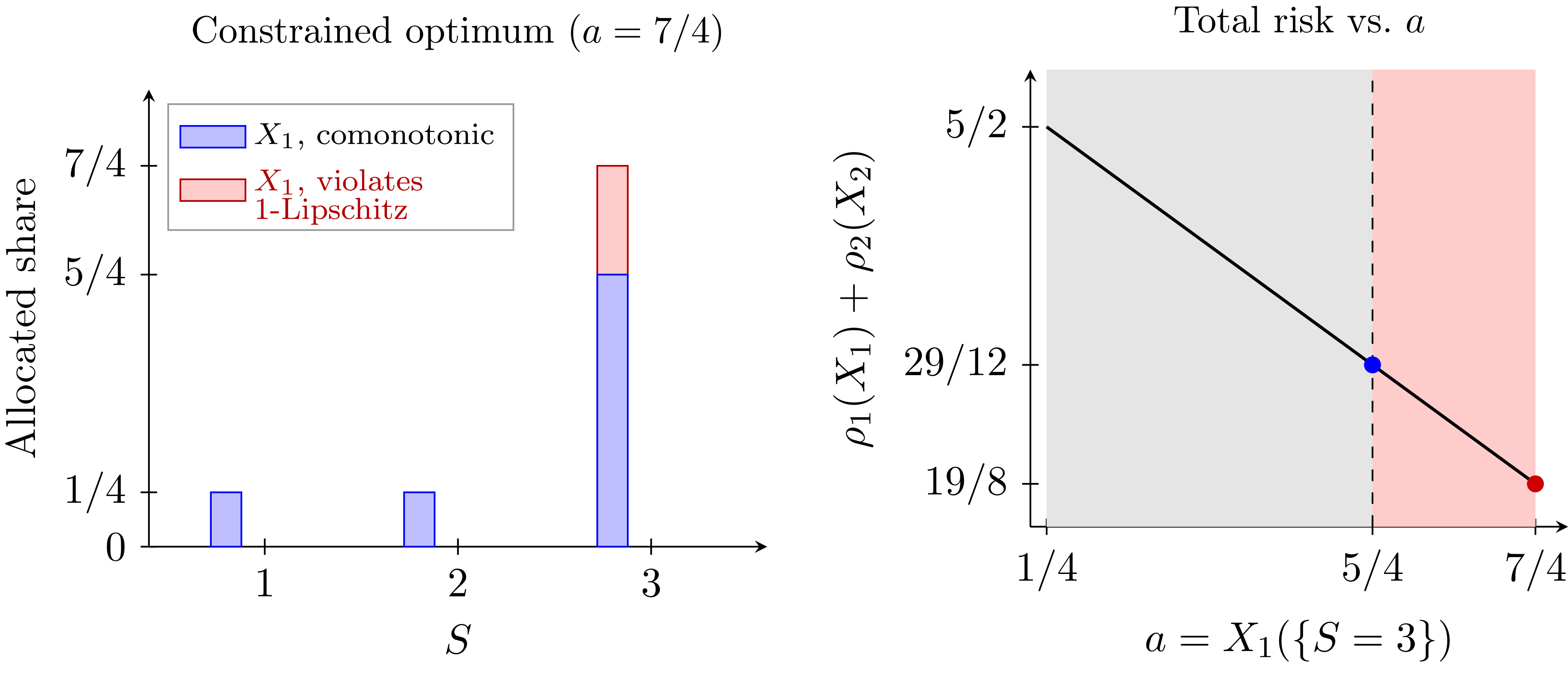
 X1=1/4
 {S≤2}
{S≤2} X1({S=3})=a∈[1/4,7/4]
 (X1,X2)
 X1({S=3})−
 X1({S=2})≤S({S=3})−S({S=2})=1
 (2,1/4)
 a∈[1/4,5/4]
 a∈(5/4,7/4]
 X2=S−X1
 19/8
19/8 a=7/4
a=7/4 29/12
29/12 a=5/4
a=5/4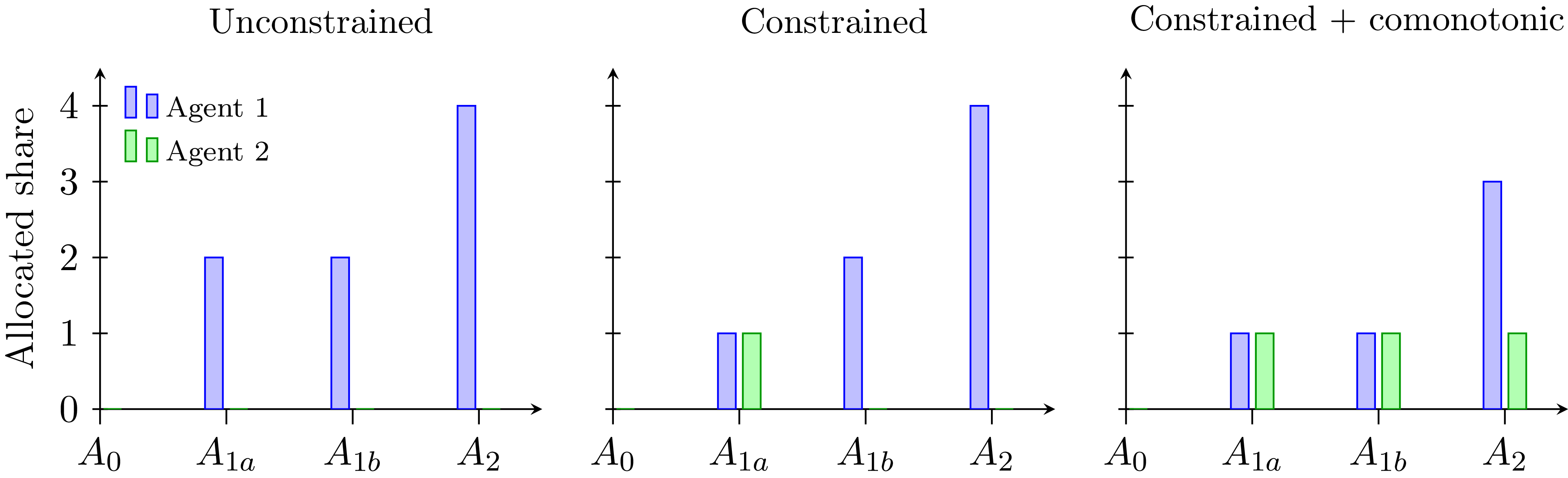
 (P(A0)=0.9925
 P(A1a)=P(A1b)=P(A2)=0.0025)
 {S=2}=A1a∪A1b
 A1a
A1a A1b
A1b 9/4>25/12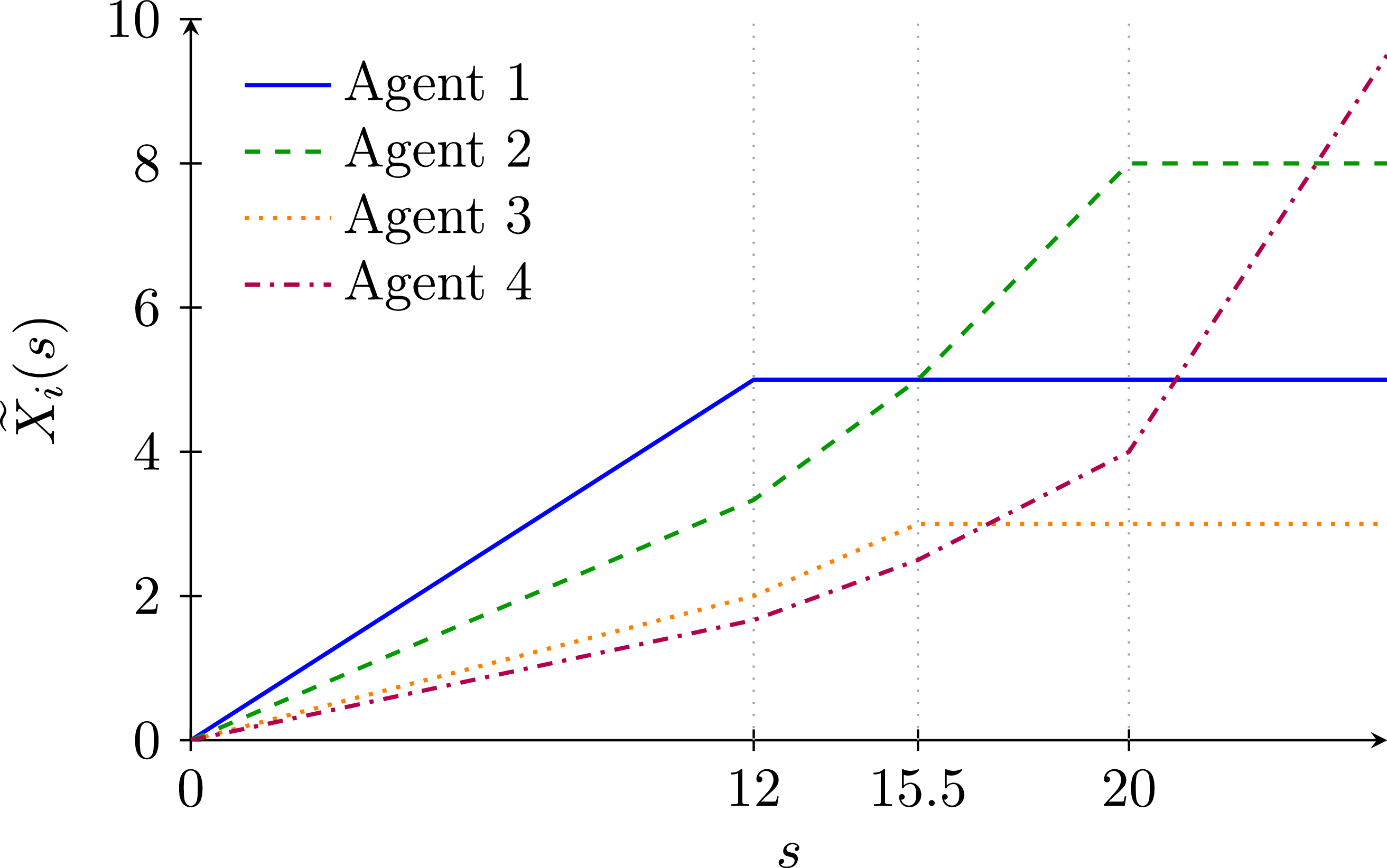
 X~i(s)
 U=(5,8,3,+∞)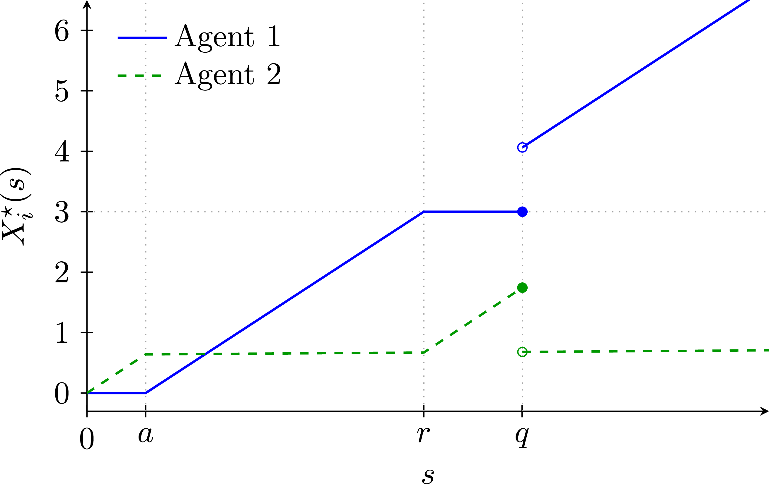
 VaR0.95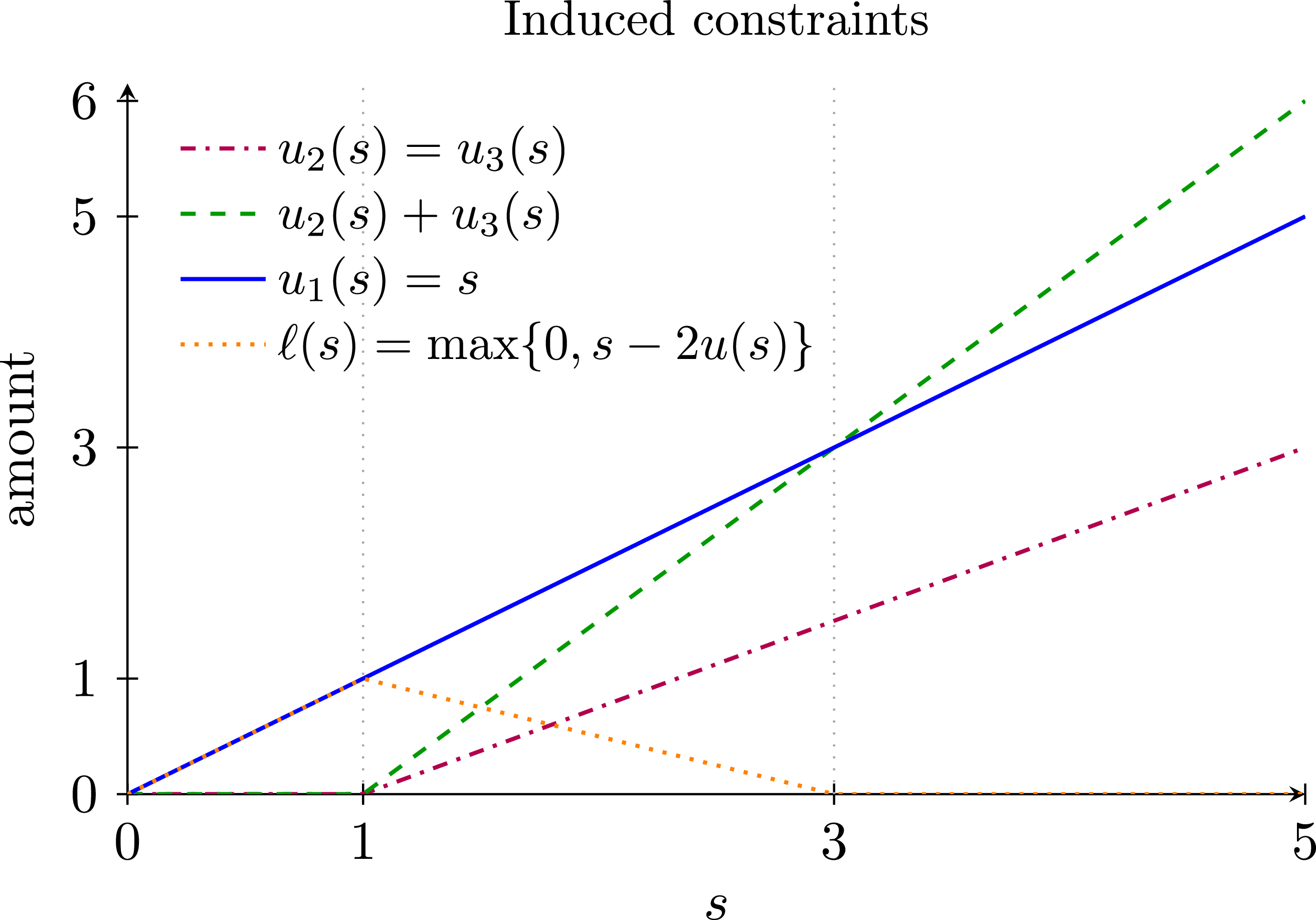
 u2(s)=u3(s)=u(s)
 u2(s)+u3(s)
 u1(s)=s
 ℓ(s)
ℓ(s)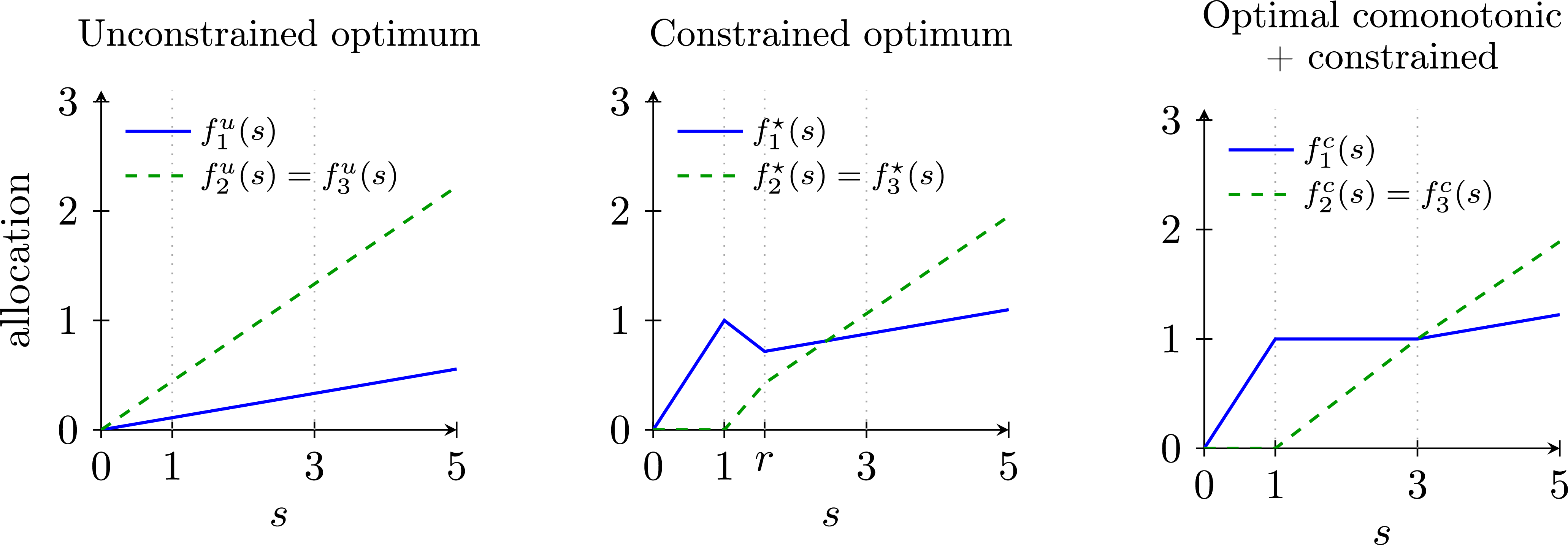
 δ=1/4
δ=1/4
 Open access

