A brief review of the Mercer & Hall example in Fisher (Reference Fisher1925)

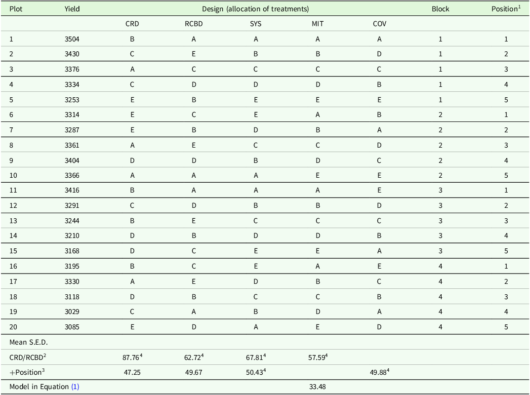
Fisher (Reference Fisher1973, p. 264) uses weights of mangold roots from a single range of 20 row plots (‘strips’; we will subsequently refer to these as plots for simplicity) by Mercer and Hall (Reference Mercer and Hall1911, Table II) to illustrate various design options as well as the analysis of variance (ANOVA). The field layout of the mangold uniformity trial comprised a 20 × 10 grid of plots, each one two-hundredth of an acre, comprising three drills and having a fixed length of 30.25 feet (9.22 m). The yields on the ten plots in a row were added up to obtain the data reported in Table II of Mercer and Hall (Reference Mercer and Hall1911). It is these data that Fisher (Reference Fisher1973, p. 264) used. The data are reproduced in Table 1. Fisher uses these data to introduce the completely randomized design (CRD) and the randomized complete block design (RCBD), considering the case of an experiment with five treatments, labelled A, B, C, D and E, and four replicates. In addition, he considers a design in systematic order, given in Figure 1, noting that (Fisher, Reference Fisher1973, 266–267)

Table 1.

Yield (weight of mangold roots; lbs) on 20 plots (‘strips’) by Mercer and Hall (Reference Mercer and Hall1911, Table II) as reported by Fisher (Reference Fisher1973, p. 264) and five overlaid designs

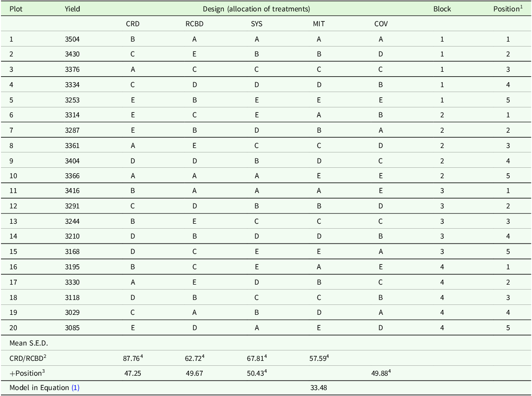
CRD, Fisher’s completely randomized design; RCBD, Fisher’s randomized complete block design; SYS, Fisher’s systematic arrangement (see Figure 1); MIT, Mitscherlich’s systematic arrangement (see Figure 2); COV, Model-based design assuming an ANCOVA model with fixed effects for blocks, treatments and position within block; Mean S.E.D., Mean standard error of a difference.

¹ Position within block; used as covariate by Fisher (Reference Fisher1973, p. 267).

² Analysed according to randomization-based model for CRD or RCBD (also for SYS and MIT).

³ Adding position number as a covariate to CRD/RCBD analysis in previous line.

⁴ S.E.D. constant for all treatment pairs.

Figure 1.

Systematic design in Fisher (Reference Fisher1973, p. 266) (SYS).

Fisher (Reference Fisher1973, p. 267) also proposed using the position number of plots within blocks (Table 1) as a covariate in an analysis of covariance (ANCOVA, another one of Fisher’s seminal contributions; Cochran, Reference Cochran, Fienberg and Hinkley1980; Senn, Reference Senn2023) in order to correct for the fertility gradient. For the RCBD, adding this covariate reduces the mean standard error of a difference (S.E.D.) from 62.7 to 49.7, indicating a linear trend within each of the four blocks. There is also some heterogeneity in the individual S.E.D.s, which range from 48.7 to 50.9. It may be noted in this regard that the systematic design (SYS) in Figure 1 has the same mean (=3) of the position numbers for each of the five treatments. If we go against Fisher’s advice and conduct an ANOVA for this design as if it were an RCBD, we find an S.E.D. of 67.8. Adding the covariate, this drops to 50.4. Notably, the S.E.D. is the same for all treatment comparisons on account of the constant position number mean for all treatments.

Mitscherlich (Reference Mitscherlich1919) proposed a systematic design (MIT), which for the example of Table 1 can be represented as shown in Figure 2. As a side note, it may be remarked that Mitscherlich wrote his little book to instruct farmers in both the execution and statistical analysis of experiments. Frequently throughout the book, he explains what a farmer would need to do in each and every step. Hence, this is literally a very early book about on-farm experimentation.

Figure 2.

Systematic design as proposed by Mitscherlich (Reference Mitscherlich1919) (MIT).

Fisher surely would have disapproved of this systematic design for the same reason that he rejected the systematic design in Figure 1 (Fisher, Reference Fisher1971, § 27). It may be conjectured that he preferred the SYS in Figure 1 for illustrating his point about the problems with systematic designs because the average position number is the same for each treatment. This pattern for the position number provides an implicit correction for a linear fertility gradient, whereas for the systematic design (MIT) in Figure 2, treatments and position numbers are fully confounded, precluding a classical ANCOVA when a block effect is included. Also see Picard (Reference Picard, Fienberg and Hinkley1980) and Speed (Reference Speed, Kotz and Johnson1991) for an account of the exchange between ‘Student’ and Fisher on systematic vs. randomized designs, in particular the discussion of the ‘Half-Drill Strip Method’ or ‘Sandwich Design’ with the systematic arrangement AB BA AB BA, which bears similarities to the SYS design in Figure 1.

Mitscherlich (Reference Mitscherlich1919) proposed an arithmetic method to adjust observed plot values for fertility differences. His key idea is best illustrated in reference to Figure 2 using plot numbers 1 to 20 as listed in Table 1 (the plots in Figure 2 are assumed to be numbered 1 to 20 from left to right). The first five plots on the left comprise the complete set of five treatments and hence may be regarded as a complete block. The average yield on these five plots with numbers 1 to 5 may, therefore, be used to correct plot yields for any fertility gradient occurring across the full range of plots. Mitscherlich (Reference Mitscherlich1919) proposed to correct all plots in the same sliding block in this way. By contrast, von Lochow and Schuster (Reference von Lochow and Schuster1961), rather than using this average yield for all plots in that block, applied the correction only to the central plot number 3 with treatment C. One may now shift the imaginary block, considered as a sliding window – or sliding block – one plot to the right so that it comprises the five plots with numbers 2 to 6 with the treatment sequence BCDEA, which again is the complete set of treatments. The average yield of these five plots can then be used to correct yield on all five plots (Mitscherlich, Reference Mitscherlich1919) or just the central plot, number, 4 with treatment D (von Lochow and Schuster, Reference von Lochow and Schuster1961). The process can be continued across the whole range of plots, each time shifting the sliding window one plot to the right. Special treatment is needed for the two border plots on each side of the range, the easiest option being to ignore these in the final analysis. Details of the arithmetic approach will not concern us here but can be found in Mitscherlich (Reference Mitscherlich1919,Reference Mitscherlich1925) and in von Lochow and Schuster (Reference von Lochow and Schuster1961). It may be added here that Mitscherlich’s key idea for local error control using sliding blocks is very similar to Fisher’s idea of blocking, and it also has similarities with the idea of nearest neighbour analysis (Piepho et al., Reference Piepho, Richter and Williams2008; Wilkinson et al., Reference Wilkinson, Eckert, Hancock and Mayo1983).

Mitscherlich did not propose a model underlying his analytical method. His arithmetic approach does suggest, however, that a model with block effects corresponding to his sliding window of five plots can be devised (Piepho and Vo-Thanh, Reference Piepho and Vo-Thanh2020). Noting that each plot is covered by five sliding blocks (v blocks in general when there are v treatments), five different block effects can be assigned to each plot. A linear model for the k-th plot can be written as

(1) \[{y_k} = \mu + \sum\limits_{j \in {M_k}} {{b_j}} + {\tau _{i\left( k \right)}} + {e_k},\]

where y _k is the response on the k-th plot, μ is an intercept, b _j is the effect of the j-th sliding block, M _k is the set of indices j of the v sliding blocks assigned to the k-th plot, i(k) (i=1,…,v) is the index of the treatment assigned to the k-th plot, τ _i(k) is the corresponding treatment effect, and e _k is a residual error, assumed to be identically normally distributed, e _k ∼ N(0,σ _e ²). If we assume block effects to be independently normally distributed, b _j ∼ N(0,σ _b ²), the model induces a spatial variance-covariance structure where the covariance between two plots drops linearly up to a distance of v − 2 intermittent plots, after which the covariance is zero (Piepho and Vo-Thanh, Reference Piepho and Vo-Thanh2020). This is because the number of sliding block effects shared between two plots k and k′ equals h _{k, k′} = max (0,v−|k−k′|), and hence, the covariance is cov(y _k ,y _k′) = h _{k, k′} σ _b ². For brevity, we will henceforth refer to this specific spatial variance-covariance structure induced by the model in Equation (1) as linear variance but should point out that this model is not identical to the linear variance (LV) model in Williams (Reference Williams1986) and Piepho and Williams (Reference Piepho and Williams2010). The main difference lies in the overlap of sliding blocks in the linear variance model used here, whereas the LV model has non-overlapping blocks and effectively has no covariance among plots in different blocks. Analysing the data in Table 1 for the systematic MIT design using the model in Equation (1), we find σˆ _b ² = 2763.18, σˆ _e ² = 1425.89 and a mean S.E.D. of 33.5.

To reiterate, it may be interjected here that Fisher probably would have criticized this kind of analysis of Mitscherlich’s design on the following grounds (Fisher, Reference Fisher1973, p. 271):

Instead, he probably would have advocated the merits of good blocking combined with properly restricted randomization (Fisher, Reference Fisher1973, p. 272):

Indeed, the CRD and RCBD provide valid analysis based on randomization theory, in which the plot values can, in fact, be regarded as fixed quantities, and randomness is induced solely by the randomization process (Fisher, Reference Fisher1971, § 21; Calinski and Kageyama, Reference Calinski and Kageyama2000; Hinkelmann and Kempthorne, Reference Hinkelmann and Kempthorne1994; Pitman, Reference Pitman1938; Welch, Reference Welch1937, § 6) [Strictly speaking, Fisher’s key argument ignores the problem of measurement error and sampling error (Hohlschuh, Reference Holschuh, Fienberg and Hinkley1980).] Exact analysis based on the randomization distribution can be approximated by analysis based on a linear model assuming normality and homogeneity of variance, and this approximation is the standard approach to analysis. Fisher (Reference Fisher1971, § 21.1) made the strong point that the exact (‘non-parametric’) analysis based on the randomization distribution should be used only as a check when the validity of the approximation is in question (also see Rosenberger, Reference Rosenberger2026, and Supplementary Material S1). In contrast to ANOVA for CRD and RCBD, there is no theory under unweighted randomization for ANCOVA [but see Cox (Reference Cox1956) and Roux (Reference Roux1982) on weighted randomization; also see Kempthorne (Reference Kempthorne1977)], and certainly no randomization theory at all for analysis of Mitscherlich’s systematic arrangement according to the spatial model in Equation (1).

Some design considerations

Interestingly, if we use a model-based approach to design generation, the spatial model in Equation (1) leads to the systematic design in Figure 2 (Piepho and Vo-Thanh, Reference Piepho and Vo-Thanh2020). This may be illustrated using the design package OPTEX (Piepho, Reference Piepho2015) (see Supplementary Material S5). The reason that the systematic design is optimal under the linear variance model is that with this configuration the average covariance of an internal plot with a treatment A with the two nearest plots with another treatment B to the right and to the left is the same for every internal plot and treatment pair under the model in Equation (1). It should be stressed, however, that there obviously is very limited randomization for this design. Every time a model-based design package were to be re-run with this model, a systematic layout as in Figure 2 would result, the only variation being a permutation of the five treatment labels. In the same vein, there is no randomization theory to justify analysis of data arising from a systematic design by the model in Equation (1). Also, there is no guarantee that the model in Equation (1) will be the best-fitting spatial model for any given dataset. The purpose of the empirical analysis described in the next section is to investigate the statistical properties of such a design-cum-analysis approach and compare it to other options.

A further model-based design option is to include the positional covariate into the model used for design generation. One such design, assuming an ANCOVA model with fixed effects for treatments, blocks and a covariate, is given in Table 1 (column labelled ‘COV’). It may be noted that the design has equal averages for position numbers for all treatments. This translates into a constant S.E.D. of 49.9 for the data in Table 1, if the usual ANCOVA model is used for analysis, which is our recommended approach. On the idea of balancing covariates in randomized experiments, including reviews of different approaches to design generation as well as to statistical analysis, see Harshaw et al. (Reference Harshaw, Sävje, Spielman and Zhang2024) and Hu et al. (Reference Hu, Hu, Ma and Rosenberger2014).

Uniformity trial data

To empirically compare the designs reviewed in the previous section, we use the wheat uniformity trial data of Mercer and Hall (Reference Mercer and Hall1911; Table V), comprising a 20 × 25 rectangular grid of plots. The size of a plot was 8 feet × 10.82 feet (2.44 m × 3.30 m). The trait is grain weight in lbs. The data is also available in the ‘agridat’ package, along with several other interesting uniformity trial datasets (Wright, Reference Wright2025). We use the individual 500 plots of the rectangular grid to overlay different designs comprising 20 plots in a single row. Thus, there are six possible selections of 20 consecutive plots per row, allowing for 6 × 20 trial areas comprising 20 plots. Three further uniformity trial datasets, also available in the ‘agridat’ package, are analysed in the Supplementary Material S2, S3 and S4, and results are briefly summarized in the main text.

Evaluation of designs using the uniformity trial data

For the design approaches discussed in ‘Designs and models’, we generate designs which are overlaid on the grid of plots in the uniformity trial data. Specifically, we extract one range of 20 contiguous plots at a time. For a row of the grid, we let a sliding window of 20 plots move through the row. This way, for a grid with 25 columns, we can extract 6 ranges per row. For each extracted range, we overlay newly generated designs and run analyses of the uniformity trial data according to the respective design, using the models described in ‘Designs and models’. For each analysis, we record the p-value of the F-test of the global null hypothesis of no treatment effects, as well as of the pairwise p-values. Based on the observed p-values, we calculate the empirical Type 1 error rate at the nominal rate of α = 5%. For valid inferences, we want the empirical to be close to the nominal Type 1 error rate.

Moreover, for each pairwise comparison, we assess both the model-based predicted variance of a difference (PRE) and the average empirical variance of a difference (EMP), using the fact that the true difference is known to be zero throughout due to the use of uniformity trial data (Baird and Mead, Reference Baird and Mead1991; Besag and Kempton, Reference Besag and Kempton1986; Müller et al., Reference Müller, Schützenmeister and Piepho2010). EMP and PRE are computed as follows (Besag and Kempton, Reference Besag and Kempton1986):

(2) ${\rm{EMP}} = {1 \over {v\left( {v - 1} \right)}}\sum\limits_{i = 1}^v {\sum\limits_{i' = 1}^v {{{\left( {{{\hat \tau }_i} - {{\hat \tau }_{i'}}} \right)}^2}} }$

(3) ${\rm{PRE}} = {1 \over {v\left( {v - 1} \right)}}\sum\limits_{i = 1}^v {} \sum\limits_{i' = 1}^v {} {\rm{Estimated}}\,{\rm{variance}}\left( {{{\hat \tau }_i} - {{\hat \tau }_{i'}}} \right)$

For valid estimates of error, we need PRE to be close to EMP. It may be conjectured that spatial covariance affects precision in systematic designs and, in particular, that treatments always appearing right next to each other in the field layout will be compared with better precision than treatments always placed farther apart. To test this conjecture, we evaluate the association of EMP with spatial distance for individual treatment pairs. For systematic designs, in which the same arrangement of treatments is used in each simulated trial, we also compare EMP to the model-based estimate (PRE) of the variance of a difference for individual pairs, i.e.

(4) $ {\rm EMP}_{ii'}=\left(\hat{\tau }_{i}-\hat{\tau }_{i'}\right)^{2}$

(5) $ {\rm PRE}_{ii'}={\rm Estimated}\,{\rm variance}\left(\hat{\tau }_{i}-\hat{\tau }_{i'}\right)$

All designs in Table 1 were randomized using simple permutations of treatment labels A–E. For the COV design, we enumerated all 993 possible designs. Here, it was assumed that a design is represented by a permutation of position numbers for each block. Without loss of generality, the permutation of position numbers for the first block will be fixed to (1, 2, 3, 4, 5). Then assuming that for each randomized design, we used a permutation of the treatment labels and aligned this with the sequence of position numbers in each block, a randomized design resulted. The process to obtain the 993 permutations was as follows:

1. i. Set the permutation of position numbers for the first block to (1, 2, 3, 4, 5). This permutation will be used for the first block in all designs.

2. ii. Generate all possible 120² permutations for Blocks 2 and 3. For each permutation, compute the sum of the position numbers for each treatment. If this yields a permutation of (7, 8, 9, 10, 11), the design is permissible. For each treatment, the position number for Block 4 is given by 12 minus the sum of the position numbers in the first three blocks.

Note that the constraint on the sum of position numbers per treatment in (ii) is required so that it is possible to obtain the same sum for each treatment when adding the position number for the fourth block. For example, if the permutation of treatment sums in (ii) is (9, 7, 11, 10, 8), adding the permutation (3, 5, 1, 2, 4) for the fourth block yields the same treatment sum for each treatment.

We tested each of the five types of design in Table 1. For each range of 20 plots selected from a uniformity trial, we performed 1000 randomizations for CRD and RCBD. For each design, randomization starts with a randomization of the treatment labels. For CRD, randomization proceeds by the random allocation of treatments to plots across the whole range, whereas for RCBD, the random allocation was done separately for each of the four blocks. For the COV design, the second step of the randomization consisted of the random selection of one of the 993 permissible designs. In our simulations, we evaluated all 993 permutations for each given range of 20 plots. For both SYS and MIT, we simulated two scenarios: (i) always use the same order (just that in Table 1), meaning there is no randomization at all and (ii) permute treatment labels in each new simulated trial. For SYS and MIT, we considered analysis based on the linear model for an RCBD. For SYS, we additionally considered analysis based on a model for an RCBD with plot position added as a covariate. For MIT, we also performed analyses based on the linear variance model in Equation (1), approximating the error degrees of freedom using the Kenward–Roger method (Kenward and Roger, Reference Kenward and Roger1997). There are only 120 permutations of the five treatment labels. In scenario (ii), we evaluated all 120 permutations of treatment labels for each given range of 20 plots.

Results of empirical comparison

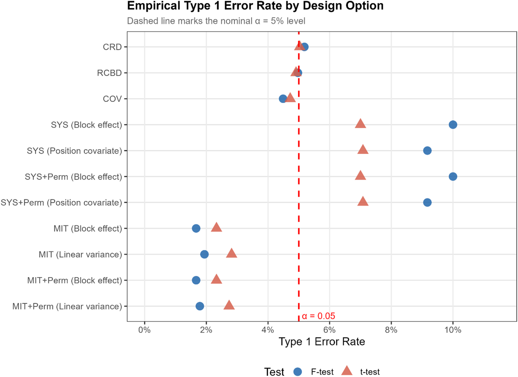
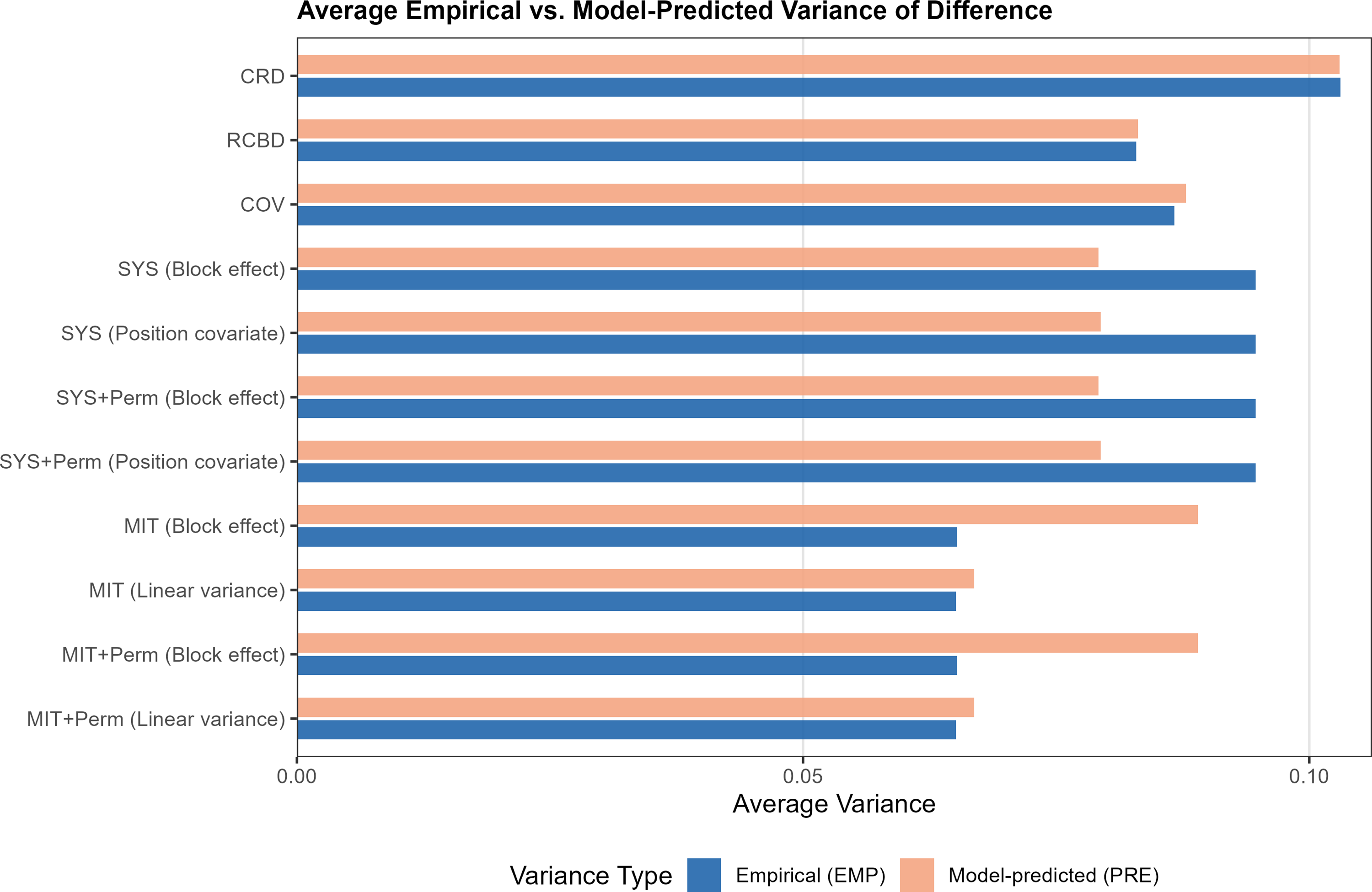
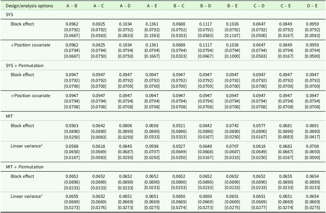
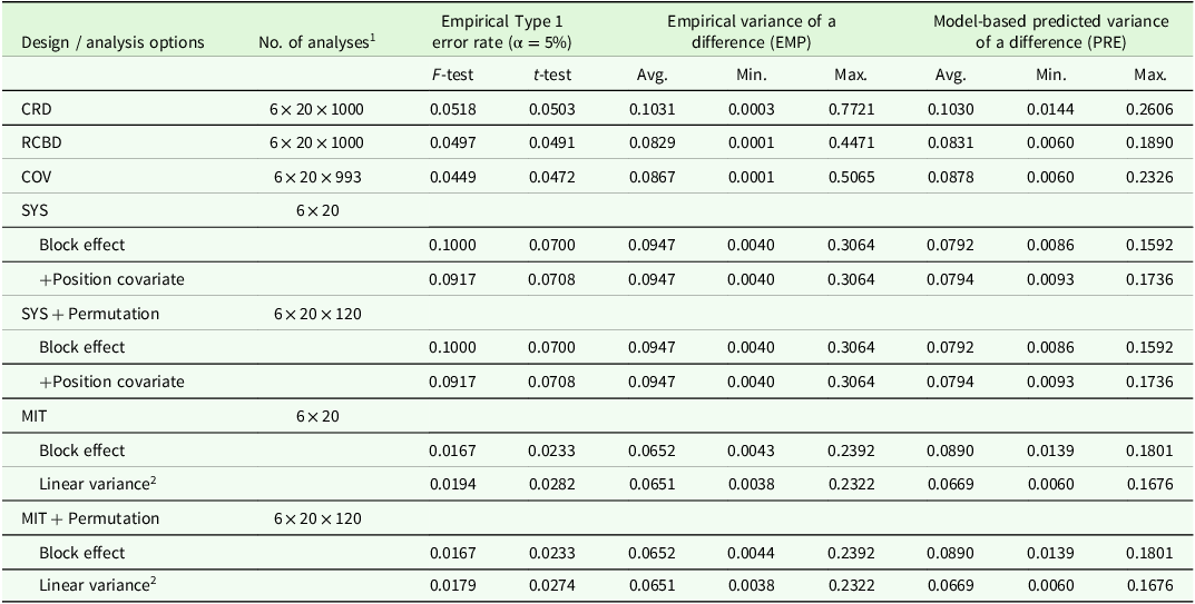
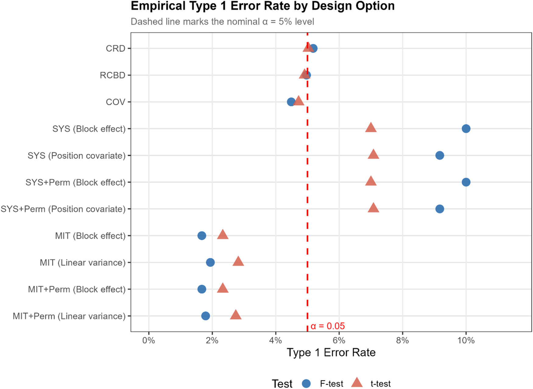
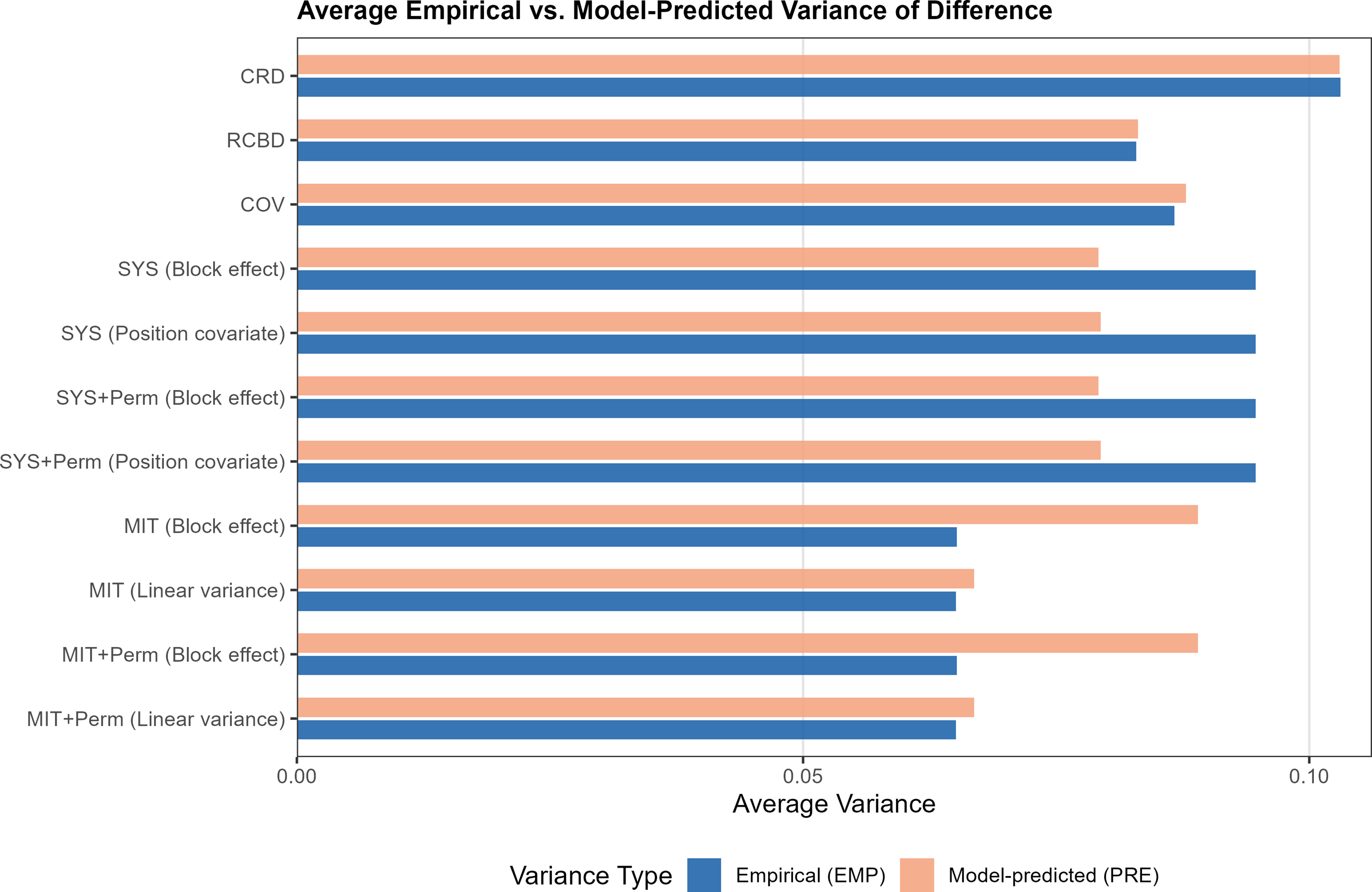
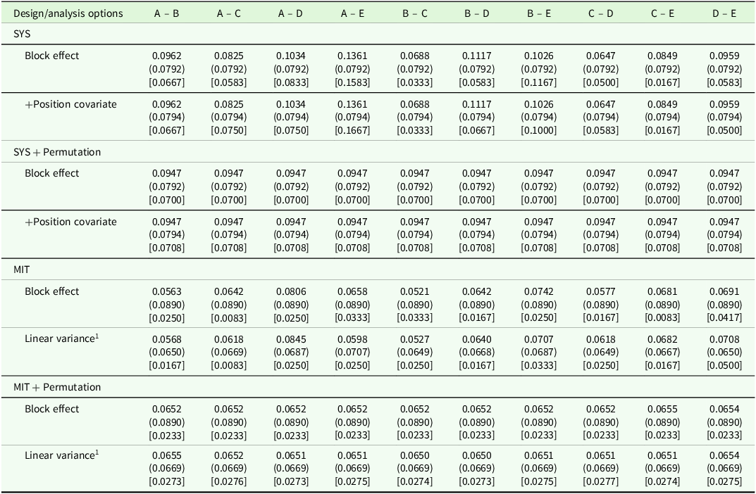
Results for EMP and PRE as per Equations (2) and (3) as well as empirical Type 1 error rates of F- and t-tests are shown in Table 2, whereas results for pairwise EMP and PRE as per Equations (4) and (5) are reported in Table 3. In addition, the Type 1 error rates of Table 2 are also displayed graphically in Figure 3 and the pairwise p-values, EMP and PRE in Figure 4. The general picture emerging from the results is that for the randomized designs CRD and RCBD as well as COV provide valid estimates of error as well as good control of the Type 1 error rate. This is not the case for the systematic designs SYS and MIT, with model-based error estimates (PRE) and Type 1 error estimates on the liberal side for SYS and on the conservative side for MIT. For MIT without permutation of treatment labels, the linear variance model in Equation (1) yields relatively good agreement between EMP and PRE on average (Table 2), but for individual comparisons, there are more marked discrepancies (Table 3), and empirical Type 1 error rates are also on the conservative side (Tables 2 and 3).

Table 2.

Empirical Type 1 error rates, empirical variance of a difference (EMP) and model-based predicted variance of a difference (PRE) using Mercer and Hall (Reference Mercer and Hall1911, Table V) wheat uniformity data for different designs and analysis options. The response is grain yield in lbs

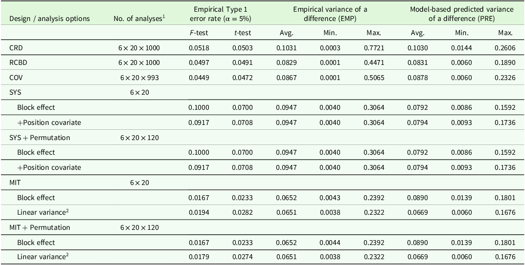
CRD, Fisher’s completely randomized design; RCBD, Fisher’s randomized complete block design; COV, Model-based design assuming an ANCOVA model with fixed effects for blocks, treatments and position within block; SYS, Fisher’s systematic arrangement (see Figure 1); MIT, Mitscherlich’s systematic arrangement (see Figure 2).

¹ Six sliding windows of 20 plots in each of 20 rows and 1000 randomizations (or all 933 or 120 permutations of treatment labels).

² Model in Equation (1).

Figure 3.

Empirical Type 1 error rates using the Mercer and Hall (Reference Mercer and Hall1911, Table V) wheat uniformity data for different design and analysis options. The response is grain yield in lbs. Linear variance: model in Equation (1). CRD, Fisher’s completely randomized design; RCBD, Fisher’s randomized complete block design; COV, model-based design assuming an ANCOVA model with fixed effects for blocks, treatments and position within block; SYS, Fisher’s systematic arrangement (see Figure 1); MIT, Mitscherlich’s systematic arrangement (see Figure 2); Perm, permutation of treatment labels for each design.

Figure 4.

Empirical variance of a difference (EMP) and model-based predicted variance of a difference (PRE) using the Mercer and Hall (Reference Mercer and Hall1911, Table V) wheat uniformity data for different design and analysis options. The response is grain yield in lbs. Linear variance: model in Equation (1). CRD, Fisher’s completely randomized design; RCBD, Fisher’s randomized complete block design; COV, model-based design assuming an ANCOVA model with fixed effects for blocks, treatments and position within block; SYS, Fisher’s systematic arrangement (see Figure 1); MIT, Mitscherlich’s systematic arrangement (see Figure 2); Perm, permutation of treatment labels for each design.

Table 3.

Pairwise empirical variance of a difference (EMP) and model-based predicted variance of a difference (PRE) for SYS and MIT designs with different analysis options. Upper figures represent EMP, middle figures in brackets represent PRE, and lower figures in square brackets represent the empirical Type 1 error rate at α = 5%. The response is grain yield in lbs. Details of the randomizations are given in Table 2 (second column)

SYS, Fisher’s systematic arrangement (see Figure 1); MIT, Mitscherlich’s systematic arrangement (see Figure 2).

¹ Model in Equation (1).

In the Supplementary Material S2, S3 and S4, we provide analyses for three further uniformity trial data: (i) a trial with spring barley, conducted in 2007 on Ihingerhof (University of Hohenheim, Germany) (Piepho and Williams, Reference Piepho and Williams2010); (ii) a wheat trial conducted in 1938 in Karnal, India (Iyer, Reference Iyer and Krishna1942); and (iii) a rice trial, conducted in 1947 in Mudon, Burma (Khin, Reference Khin1950). The results are broadly similar to those for the Mercer and Hall data, with CRD, RCBD and COV providing approximately valid estimates of error, whereas SYS and MIT prove to be invalid. All four uniformity trial datasets considered in this paper are also available in the ’agridat’ package (Wright, Reference Wright2025).