


1. Introduction
As climate change accelerates glacial melt, greater volumes of water are flowing over, within and beneath glacier systems (Huss and Hock, Reference Huss and Hock2018), and supraglacial water routing pathways are altered. These pathways and connections between supra- and subglacial systems have important implications for glacier dynamics (through the transfer of water and heat; Cuffey and Paterson, Reference Cuffey and Paterson2010; Pitcher and Smith, Reference Pitcher and Smith2019), water storage in the system and timing of glacier contributions to both sea-level rise and local river systems (Chu, Reference Chu2014; Wyatt and Sharp, Reference Wyatt and Sharp2015; Miles and others, Reference Miles2017; Bell and others, Reference Bell, Banwell, Trusel and Kingslake2018). Mapping these water pathways is one means to better understand the glacier hydrologic system and its evolution (Chu, Reference Chu2014; Wyatt and Sharp, Reference Wyatt and Sharp2015; Bell and others, Reference Bell, Banwell, Trusel and Kingslake2018; Smith and others, Reference Smith2021).
Mapping supraglacial hydrological features and their changes over time is not straightforward and has been the focus of many studies. Automated or semi-automated methods have been used to identify supraglacial streams (e.g. Karlstrom and Yang, Reference Karlstrom and Yang2016; Lu and others, Reference Lu2020), moulins (e.g. Clason and others, Reference Clason, Mair, Burgess and Nienow2012) and supraglacial lakes (e.g. Yang and others, Reference Yang, Smith, Chu, Gleason and Li2015; Miles and others, Reference Miles2017). Following Yang and Smith (Reference Yang and Smith2013), many studies use a modified water index (described below) to classify actively flowing streams, moulins and water-filled lakes. This approach has been applied successfully on the Greenland Ice Sheet, as well as large ice caps in the Canadian Arctic (e.g. Yang and Smith, Reference Yang and Smith2013; Smith and others; Lu and others, Reference Lu2020). An alternative approach uses digital terrain models (DTMs) to identify likely flow pathways based on surface slope and aspect (Teegavarapu and others, Reference Teegavarapu, Viswanathan and Ormsbee2006; Yang and others, Reference Yang, Smith, Chu, Gleason and Li2015; Rippin and others, Reference Rippin, Pomfret and King2015; King and others, Reference King, Hassan, Yang and Flowers2016; Yang and others, Reference Yang2019). The wide availability of DTMs and tools for surface analysis mean that this approach can be applied where multi-spectral data are not available (King and others, Reference King, Hassan, Yang and Flowers2016), and it has been found to produce a connected supraglacial drainage network model that broadly matches stream networks visible in aerial imagery (Yang and others, Reference Yang, Smith, Chu, Gleason and Li2015; King and others, Reference King, Hassan, Yang and Flowers2016; Yang and others, Reference Yang2019). These two methods do not represent the same stream networks, however, with the former mapping active hydrology and the latter mapping all potential flow pathways (King and others, Reference King, Hassan, Yang and Flowers2016; Yang and others, Reference Yang2019).
These automated and semi-automated methods can be limited by spatial and spectral resolution, depending on the type of data that are available, and are sensitive to threshold choices for masking non-stream pixels (i.e. Yang and Smith, Reference Yang and Smith2013; King and others, Reference King, Hassan, Yang and Flowers2016). Where high spatial resolution (sub-metre) satellite and aerial imagery are available, streams on smaller glaciers (outside of the major ice sheets and ice caps) may be identified with automatic classification, but these data are often not accessible. Decaux and others (Reference Decaux, Grabiec, Ignatiuk and Jania2019) found that the index-based method failed to identify streams in ‘dirty’ ice, and also where streams are much smaller than in Greenland where the method has been most widely used. The increase in aerial surveying with commercial digital cameras is opening new possibilities for high-resolution mapping, but spectral indices also do not transfer directly to these platforms which do not record reflectance values, complicating the application of existing automatic classification methods. Rippin and others (Reference Rippin, Pomfret and King2015) used a DTM from a drone survey with major topographic trends removed to identify surface depressions consistent with a stream network. Yang and others (Reference Yang2018) use drone survey data to qualitatively validate automated methods but did not apply those automated methods directly to drone imagery. Rippin and others (Reference Rippin, Pomfret and King2015) note that this ultra-high-resolution, on-demand imagery presents opportunities for examining dynamic channel changes through identification of meander cut-offs, abandoned channels and the acquisition of repeat imagery.
The identification of hydrologic sinks, where water can drain into the glacier or glacier bed, is of particular importance in mapping supraglacial hydrology because these locations form the connections between the supra- and sub-glacial systems and disrupt the continuous flow of water through modelled pathways. In the DTM-based flow pathway modelling approach, filling depressions in the DTM is often the first step but may mask true sinks. Yang and others (Reference Yang, Smith, Chu, Gleason and Li2015) found that drainage networks simulated with hydrology tools and moderate-resolution (30–40 m) DTMs fail to capture most true moulins, since these features are small in comparison to pixel sizes. Consequently, the drainage network connectivity can be overestimated using a DTM-based method alone. One alternative way of addressing this is to use a sink-overflow model, which allows depressions to remain and water to drain between sink catchments (e.g. Arnold, Reference Arnold2010; Banwell and others, Reference Banwell, Arnold, Willis, Tedesco and Ahlstrøm2012). More commonly sinks (in particular moulins) are identified manually and used as drainage points for catchments (e.g. Smith and others; King and others, Reference King, Hassan, Yang and Flowers2016; Yang and others, Reference Yang2018). In most studies, however, the limitations of identifying sinks lead to these being manually identified, a process which can be time consuming.
Many studies using automated methods also rely on manual digitization for validation and accuracy assessments (e.g Yang and Smith, Reference Yang and Smith2013; King and others, Reference King, Hassan, Yang and Flowers2016; Lu and others, Reference Lu2020). Lu and others (Reference Lu2020) found that gaps in the automated water index approach for stream delineation result in 13% less total stream length compared to manually digitized streams. King and others (Reference King, Hassan, Yang and Flowers2016) found that manually digitized stream networks matched flow-routing models at over 90% for high-order streams (i.e. largest stream branches), but correspondence dropped for lower order streams. The discrepancies were largely due to the choice of channel initiation threshold (the value at which pixels are classified as streams).
Manual identification of supraglacial features (e.g. Lampkin and Vanderberg, Reference Lampkin and Vanderberg2014; Wyatt and Sharp, Reference Wyatt and Sharp2015; Miles and others, Reference Miles2019; Decaux and others, Reference Decaux, Grabiec, Ignatiuk and Jania2019) requires the use of the elements of image interpretation (Supplementary Appendix A; Shellito, Reference Shellito2018). This kind of image interpretation allows experienced users to discern features from remotely sensed images but involves decisions that can be subjective (Decaux and others, Reference Decaux, Grabiec, Ignatiuk and Jania2019). Individuals who are not content experts may have difficulty evaluating feature characteristics and even experienced users may not consistently interpret features (Shellito, Reference Shellito2018). Few studies have defined criteria for mapping supraglacial features in manual image interpretation, complicating comparisons between studies where different methods may have been employed. King and others (Reference King, Hassan, Yang and Flowers2016) and Lampkin and Vanderberg (Reference Lampkin and Vanderberg2014) give similar definitions for identifying streams in DEMs and panchromatic imagery: ‘Features that were rectilinear in morphology and demonstrated relative high contrast in reflectance between the presumed channel and the surrounding ice were mapped as channels’ (Lampkin and Vanderberg, Reference Lampkin and Vanderberg2014).
Given that there is little transparency in current methods for mapping supraglacial features manually, and even studies employing automated classification strategies often fall back on manual methods of identifying moulins and verifying classifications, we set out to create a standardized decision-making framework for semi-automated mapping of supraglacial hydrological features including streams, moulins and crevasses. In this framework we build on previous work which used DTMs for flow routing to produce an initial hydrologic network that can be manually checked. We chose the flow routing method over the water index method because it is more readily applied to imagery without spectral information. As discussed above, relying on the flow routing method alone can introduce problems, and so we set up a classification system for these modelled flow pathways. Each of the features in our framework is identified through a series of decision trees. By clearly defining characteristics for each feature, we also hope to improve consistency in feature mapping for comparison between studies in the future.
Rather than producing exhaustive maps of surface features, we define features as hydrologically significant when they are part of the connected hydrological network on a glacier and include these in our maps. This allows us to avoid an exhaustive search of the glacier surface when identifying moulins and crevasses which may connect to the sub-glacial system. This framework is designed for use by individuals with beginner level image-interpretation skills and alleviates the need for expert users to create these hydrological maps.
2. Study sites
The framework we describe was developed at Nàłùdäy (Lowell Glacier) in Yukon, Canada: traditional territory of the Champagne and Aishihik First Nations (Fig. 1)(Champagne and Aishihik First Nations, 2021). Nàłùdäy is a large valley glacier in the St. Elias Mountains, ~65 km long and 4 km wide, ranging in elevation from 600 m above sea level (a.s.l.) at the terminus to 1500 m a.s.l. in the upper accumulation area. Nàłùdäy is a surge-type glacier whose past advances have significantly impacted the lives of indigenous people in the area by cutting off the Alsek River and disrupting fish migration; the Dákwanjè (Southern Tutchone) name roughly translates to ‘fish stop’ (Champagne and Aishihik First Nations, 2021). Nàłùdäy was chosen for this work because it is part of a larger study in the St. Elias region, where aerial photogrammetric surveys have been conducted, and the supraglacial hydrology is of particular interest. An Environment Canada weather station located in Haines Junction, 60 km north of the glacier, has recorded average daily summer (May–September) temperatures of 10.5°C from 2017–2019 (with a mean daily range of 1.1–21.6°C). In 2018, average late season melt was 2.1 m across the ablation zone (0.041 m d−1; Hill and others, Reference Hill, Dow, Bash and Copland2021).
The framework for mapping supraglacial hydrology described below was developed at Nàłùdäy, Yukon (a) and tested at Thores Glacier, Nunavut (b). Both (a) and (b) show mapped hydrology and orthomosaics overlain on top of ESRI basemap imagery from Maxar. See Figures 7 and 9 for meaning of coloured lines.
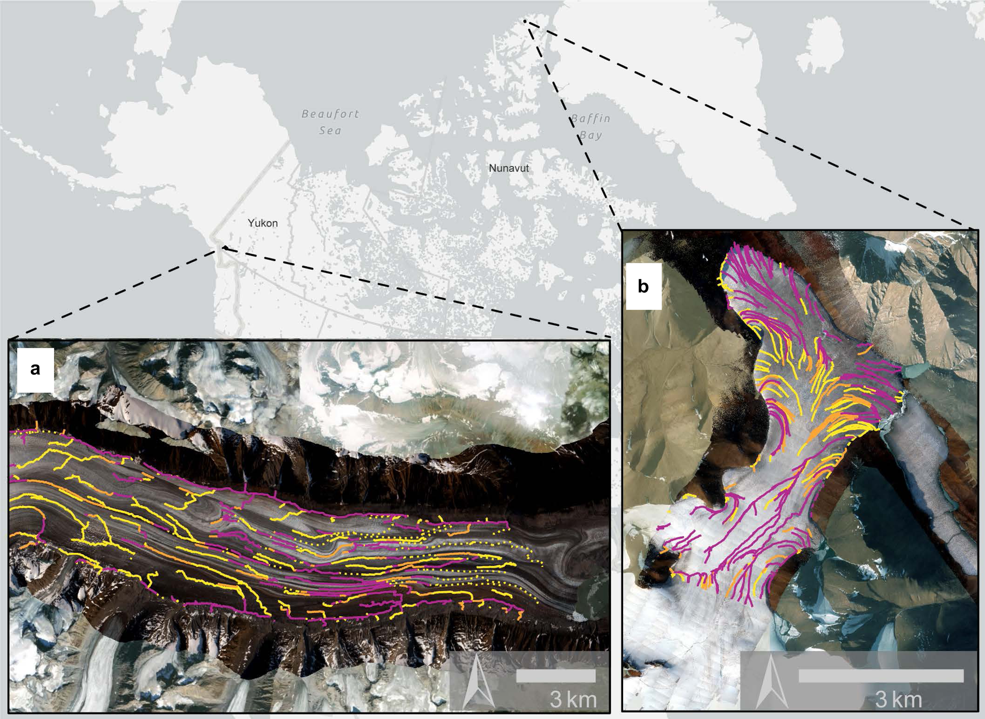
In order to assess the framework in a different context, we apply it on Thores Glacier, Nunavut, Canada. We chose this site because it has a different climatic setting (high-Arctic versus sub-Arctic) and morphology compared to Nàłùdäy. In addition, Thores was surveyed as part of another study in 2019 and the same type of aerial survey data was available as from Nàłùdäy. Thores Glacier is located on Northern Ellesmere Island in the Canadian Arctic, Inuit Nunangat (Fig. 1). It is ~14 km long, with a width of ~1.4 km, and ranges from 650 to 1100 m a.s.l. in elevation. A weather station located on nearby Ward Hunt Island, 100 km north of Thores, recorded average summer (July–August) temperatures of 0.71°C between 2017 and 2019 (with a range of −3.7 to 8.0°C; CEN, 2020).
Thores is a shorter and steeper glacier than Nàłùdäy; the average centreline surface slope in the lower 26 km of Nàłùdäy is 2.5%, while the slope of Thores is 6.3% for the lower 7 km. Nàłùdäy is heavily crevassed in places and has looped medial moraines as a result of past surging. Thores, in contrast, has few crevasses and little surface debris. The average air temperatures, slope and presence of debris all impact the volume of melt water produced; which in conjunction with crevasse density will lead to development of different surface drainage networks.
3. Data
Our framework requires orthorectified red, green, blue (RGB) imagery and a DTM spanning the extent of the glacier. Multi-band imagery allows for band ratios to be applied, which helps to interpret hydrological features (Shellito, Reference Shellito2018). For optimal supraglacial feature identification, the aerial imagery and DTM should be synchronous in time and space, and be of sufficiently high-resolution to identify surface features. The required resolution depends on the size of features at a site; we recommend pixel sizes no larger than half the size of features being mapped (Hengl, Reference Hengl2006). This allows for clear identification of feature boundaries in imagery and topography in the DTM which reflects feature morphology.
We developed the framework at Nàłùdäy using an orthorectified image mosaic and DTM, both 0.5 m resolution, collected over the lower 200 km2 of the glacier in July 2019. The framework was then applied in two contexts: one with readily available data (described below) and one at Thores Glacier, a glacier with different surface and hydrological characteristics. At Thores Glacier the framework was applied using an orthorectified image mosaic and DTM, 1 m resolution, collected over the lower 22 km2 of the glacier in July 2019.
High-resolution imagery over both glaciers was collected using a Nikon D850, a 45 mega-pixel DSLR camera, with a 24 mm lens during a piloted aircraft flight. The camera was connected via the hot shoe to a Trimble R7 GNSS receiver, which recorded an event marker for each image; these positions were post-processed using Natural Resources Canada's Precise Point Positioning service. Using the structure-from-motion software Agisoft Metashape Professional 1.5, photos were aligned and georeferenced using positions of each image. A final dense point cloud was derived and used to generate a DTM at 0.5 m resolution by averaging the elevation of points within each gride cell. The DTM was used to orthorectify images and generate a mosaic; the mosaic pixels were not blended in construction, so individual pixels represent information captured by a single image in the flight. Blending pixels in the generation of orthomosaics has been shown to result in a loss of information about the scene (Wang and others, Reference Wang2020).
The application of the framework with readily available data was conducted using imagery and a DTM of lower resolution than those we used to develop the approach which are freely available online. For this application, we used ArcticDEM v 3.0 from the Polar Geospatial Center and ESA Sentinel-2 imagery available at 10 m resolution. ArcticDEM is a pan-arctic 2 m DTM constructed from stereo imagery acquired by the DigitalGlobe satellites (Porter and others, Reference Porter2020). ArcticDEM is available both as ‘strips’ derived from single image pairs, and as a mosaic which includes information from co-registered and blended strips. Although strips from a single date are preferable for applying our framework, a single strip does not cover the whole of Nàłùdäy, so instead we used the mosaic for testing. By using these readily available data, we were able to apply the approach in a context which future users may use it. Recognizing that high-resolution aerial survey data are not available in many cases, we believe this represents a more realistic use-case for employing the approach. The dates of strips blended over Nàłùdäy range from winter 2013 to spring 2017, with a majority in winter and spring 2017. We used imagery from the Sentinel-2 Multispectral Instrument captured on 17 July 2016. This date was chosen to match the date of the ArcticDEM as closely as possible, while minimizing snow and cloud cover over Nàłùdäy. The data used in this test were asynchronous in time and had lower resolution than the aerial imagery, which allowed us to test the framework under non-ideal conditions and shed light on the framework performance with readily available data.
We derive several additional products from the DTM and RGB imagery, which we use in the development of the mapping framework. These products were derived in ArcGIS Pro v2.3 using the Hydrology Toolset (Esri, 2020), but are described below such that they can be produced with other software.
3.1 Stream model
Similar to other work using GIS-based methods for stream analysis (Banwell and others, Reference Banwell, Arnold, Willis, Tedesco and Ahlstrøm2012; Arnold and others, Reference Arnold, Banwell and Willis2014; King and others, Reference King, Hassan, Yang and Flowers2016), we first derive a model of the glacier surface drainage network based on the DTM (stream model). The stream model derived from the DTM shows theoretical flow pathways that water is predicted to take on the glacier surface, which may or may not represent actual streams. Where this includes surrounding terrain, we also include ice-marginal streams relevant to the glacier hydrological network. There are several intermediate steps to producing the stream, which we performed as follows:
1. Filling sinks where drainage directions (as defined below) are undefined. Similar to other studies, without this step the drainage network was found to be disjointed (Yang and others, Reference Yang, Smith, Chu, Gleason and Li2015; Miles and others, Reference Miles2017). Sinks are cells or groups of spatially-connected cells in which the flow direction cannot be calculated because there are no downslope neighbouring cells. Sinks in DTMs may represent true topographic depressions in a modeled surface or may be errors associated with the DTM. Filling sinks in the DTM ensures drainage connectivity but also masks true depressions. We found that adjusting the threshold value (difference between sink and surroundings) to leave some sinks unfilled produced a flow accumulation layer which had little hydrological connectivity, regardless of the value we chose. To obtain a stream model with continuous streams all DTM depressions were initially filled.
2. Calculating flow direction at each cell. We used the D8 method for this calculation, which identifies the direction of steepest descent from each grid cell to one of its eight neighbouring cells (O'Callaghan and Mark, Reference O'Callaghan and Mark1984).
3. Calculating flow accumulation at each cell. Flow accumulation is the number of cells flowing into a given cell, using the flow direction calculation. This means that higher values have larger upslope drainage catchments, which we take advantage of in masking non-stream cells following this calculation.
4. A binary raster of stream and non-streams cells is created from the flow accumulation raster. The final stream model is very sensitive to the selection of the threshold value for classification of cells as stream or non-stream. A low threshold value will include cells with smaller catchments that may not be streams, while a high value will include only the cells with larger catchments and may exclude small actual streams. We determined the threshold for classification by examining the quantiles of the flow accumulation values. Beginning with four quantile groups, we increased the number of groups and noted the value of the boundary between the two smallest groups. With larger numbers of groups the value stabilized and this was used as the threshold for classification. This value must be derived for individual datasets and this quantile-based method avoids a circular approach of choosing the threshold value by matching streams visually. For the framework development data at Nàłùdäy the value was found to be 421 114 which is equivalent to 0.1 km2 of upslope drainage area (0.5 m resolution). In the test case using ArcticDEM data with 2 m resolution, this boundary value was 38 145 pixels, or 0.15 km2 of upslope drainage area.
5. The binary stream raster was converted to polylines to produce the final stream model.
3.2 Sink model
To identify true hydrologic sinks (such as moulins, crevasses and depressions), we produce a dataset which identifies sinks that were filled when producing the stream model described above so they can be visualized alongside the stream model. In glacial environments, sinks may represent points where water enters the englacial and subglacial drainage systems (Banwell and others, Reference Banwell, Arnold, Willis, Tedesco and Ahlstrøm2012; Yang and others, Reference Yang, Smith, Chu, Gleason and Li2015; King and others, Reference King, Hassan, Yang and Flowers2016). This model is produced following steps 1 and 2 from the stream model, where the filled DTM uses a filling threshold equal to the resolution of the DTM (i.e. sinks greater than one pixel in depth remain unfilled). From this flow direction raster, cells with no downslope neighbouring cells are classified as sinks.
3.3 NDWIice
The normalized difference water index (NDWI) model is commonly used to identify water in multispectral imagery (McFeeters, 1996). The standard NDWI is the normalized ratio of the near infrared and green bands. However it is not ideal in glacial environments because melting ice, snow and firn have low reflectance in the near infrared wavelengths (Yang and Smith, Reference Yang and Smith2013). Yang and Smith (Reference Yang and Smith2013) define a NDWI ratio using the blue and red bands, which we employ in this study.
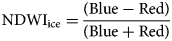
The NDWIice is dimensionless and ranges from −1 to +1, where high NDWI values correspond to liquid water and low values correspond to dry snow and firn.
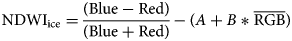
Aerial imagery collected with standard digital cameras is not true reflectance data in RGB bands, which means that variations in lighting conditions between images can lead to two images having different band values at the same location. This can be easily seen in some orthomosaics, where surfaces appear to have dark and light patches (Fig. 9). Calculating NDWIice using digital numbers from camera sensors is thus strongly dependent on image brightness, unrelated to any actual surface characteristics. To address this problem, we correct the NDWI using the average RGB value ($\overline {{\rm RGB}}$ ) for each glacier as a whole, which is linearly related to NDWI (Fig. 2).
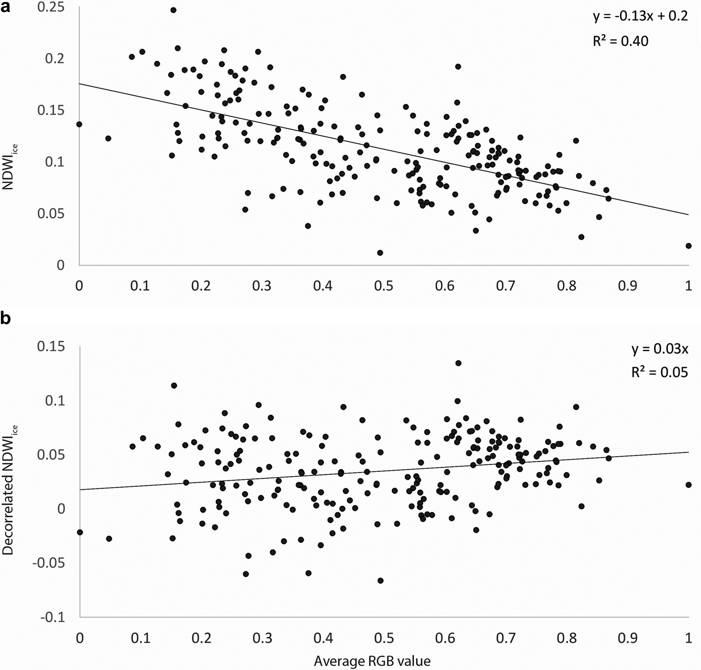
(a) The relationship between NDWIice and $\overline {{\rm RGB}}$ at Thores Glacier; the linear best fit line was used to decorrelate the two variables (Eqn 2). (b) The relationship between NDWIice and $\overline {{\rm RGB}}$
 after decorrelation.
Where A and B are coefficients determined by fitting a linear relationship between $\overline {{\rm RGB}}$ and NDWIice. This method is novel and was designed to decorrelate lighting and NDWIice by removing the variability in NDWIice that depends on image brightness. We found that $\overline {{\rm RGB}}$
 was more strongly related to NDWIice than $\sum {{\rm RGB}}$
 . We visualize the NDWIice raster in grayscale and refer to the relative shades of pixels in definitions below.
3.4 Hillshade model
We derive two shaded relief rasters from the DTM. The lighting direction was set to be perpendicular to the general flow direction of the glacier (North and South for Nàłùdäy; East and West for Thores) and a low solar altitude was chosen, both to amplify the appearance of relief in streams (which generally flow parallel to the glacier flow direction). We produce the hillshade model without including shading from surrounding terrain, this means that the shading in the model is from local relief only. The resulting hillshade model shows a grayscale representation of the vertical glacier surface relief.
4. Mapping framework
The framework for mapping supraglacial hydrology is structured as a series of decision points for the user with the stream model as a starting point (text descriptions of the decision points are included in Supplementary Appendix B). Four types of features are mapped: streams, moulins, crevasses and ice cauldrons. This mapping framework is aimed at identifying hydrologically significant features, rather than an exhaustive map of features that are present. We assume that the stream model will include most reaches of the drainage network, and those that are missed are likely small or ephemeral and thus carry less water in the system.
The framework described below was developed collaboratively by a content expert in glaciology (Bash) and a GIS user (Shellian) with little experience in glaciology. This allowed us to refine the framework in a way that was easy to apply by non-experts, while utilizing expert knowledge in the development phase.
4.1 Supraglacial streams
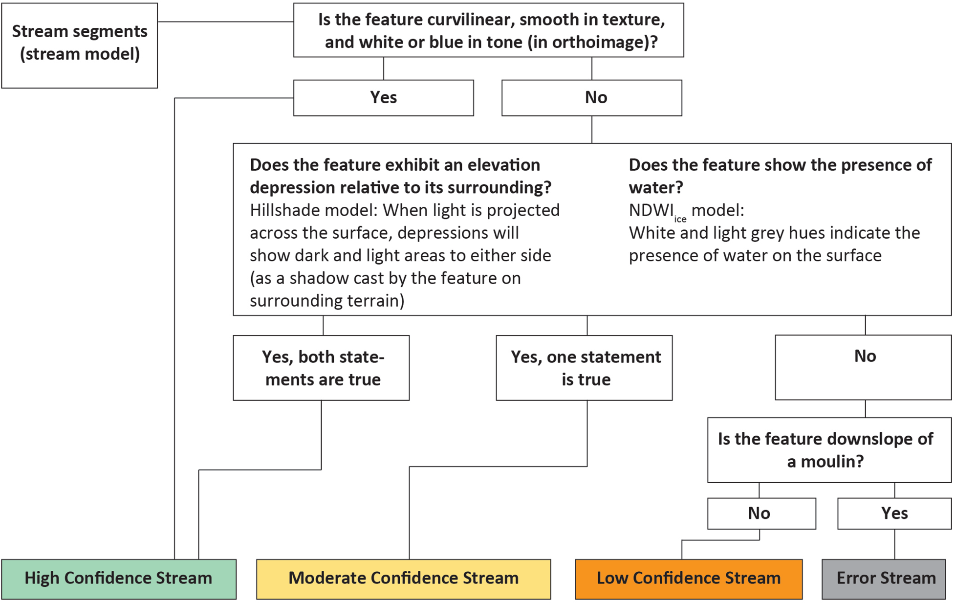
Beginning with the polylines of the stream model we examine sections of the modelled network and classify each section in one of four classes (Fig. 3; and Supplementary Appendix B) – high confidence streams (Fig. 4), moderate confidence streams, low confidence streams and error streams (additional example figures in Supplementary Appendix B).
Decision tree for classifying stream model polylines. Sections of the stream model network are examined and classified in one of four classes – high confidence streams, moderate confidence streams, low confidence streams and error streams.
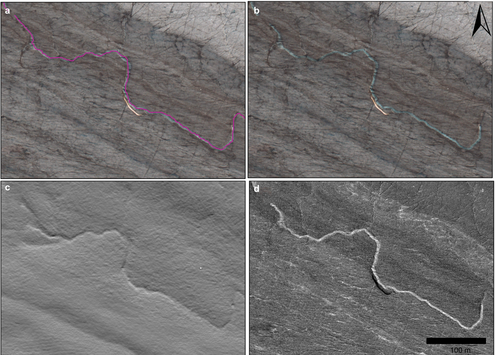
An example from Nàłùdäy of (a) a delineated high-confidence stream shown over the high-resolution orthmosaic (0.5 m). (b) High-resolution orthomosaic without stream delineated, illustrating that high-confidence streams are characterized by smooth texture and white or blue tone; (c) Hillshade model, showing the brightness change consistent with a depression at the stream location; (d) NDWIice model, showing a light tone relative to the surroundings at the stream location.
The stream classes are determined by the feature's characteristics and association with other features. We use terminology of image interpretation to define streams as being curvilinear, smooth in texture and white or blue in tone relative to its surroundings. Curvilinear lines have few sharp angles, and smooth image texture is characterized by homogenous pixels. When these conditions are all met, a stream is classified as high-confidence, if any of these conditions are not met, then the hillshade model, NDWIice, and sink locations are used to determine the classification (Fig. 3). Further written description of the decision process can be found in Supplementary Appendix B. In some cases error streams may be abandoned channels, but within this framework we do not consider these to be hydrologically significant.
After polylines in the stream model were classified into the above stream classes, the starting points (upstream) of high-confidence streams were manually verified. Starting points for high-confidence streams were extended up-glacier if the up-glacier feature exhibits a brightness consistent with the features’ shape (elevation depression) relative to its surrounding in the hillshade model; and the feature exhibits a light grey or white tone relative to its surroundings, indicating the presence of water in the NDWIice raster.
4.2 Moulins
In the process of classifying streams, we also identify hydrologically connected moulins (Fig. 5). These are defined as being located at the terminus of high-confidence streams, with a rounded shape and difference in tone relative to surroundings, as well as either coinciding with a sink or showing an indication of water in NDWIice, or both. As discussed above, moulins are an important component of the supraglacial hydrologic system, given that they allow water to enter the subglacial system and disrupt flow paths on the glacier surface. Moulins are often associated with crevasses, faulting and lake drainages (e.g. Catania and others, Reference Catania, Neumann and Price2008; Banwell and others, Reference Banwell, Arnold, Willis, Tedesco and Ahlstrøm2012; Phillips and others, Reference Phillips, Finlayson and Jones2013), where flowing water or structural controls are enough to fracture ice. As such, moulins require significant water input to form and thus, when they are active, are most likely to be connected to supraglacial streams (rather than occurring in isolation). There are many examples of moulins occurring in isolation (Banwell and others, Reference Banwell, Arnold, Willis, Tedesco and Ahlstrøm2012; King and others, Reference King, Hassan, Yang and Flowers2016), however, we consider isolated and inactive moulins not to be hydrologically significant in this framework and these are not mapped.
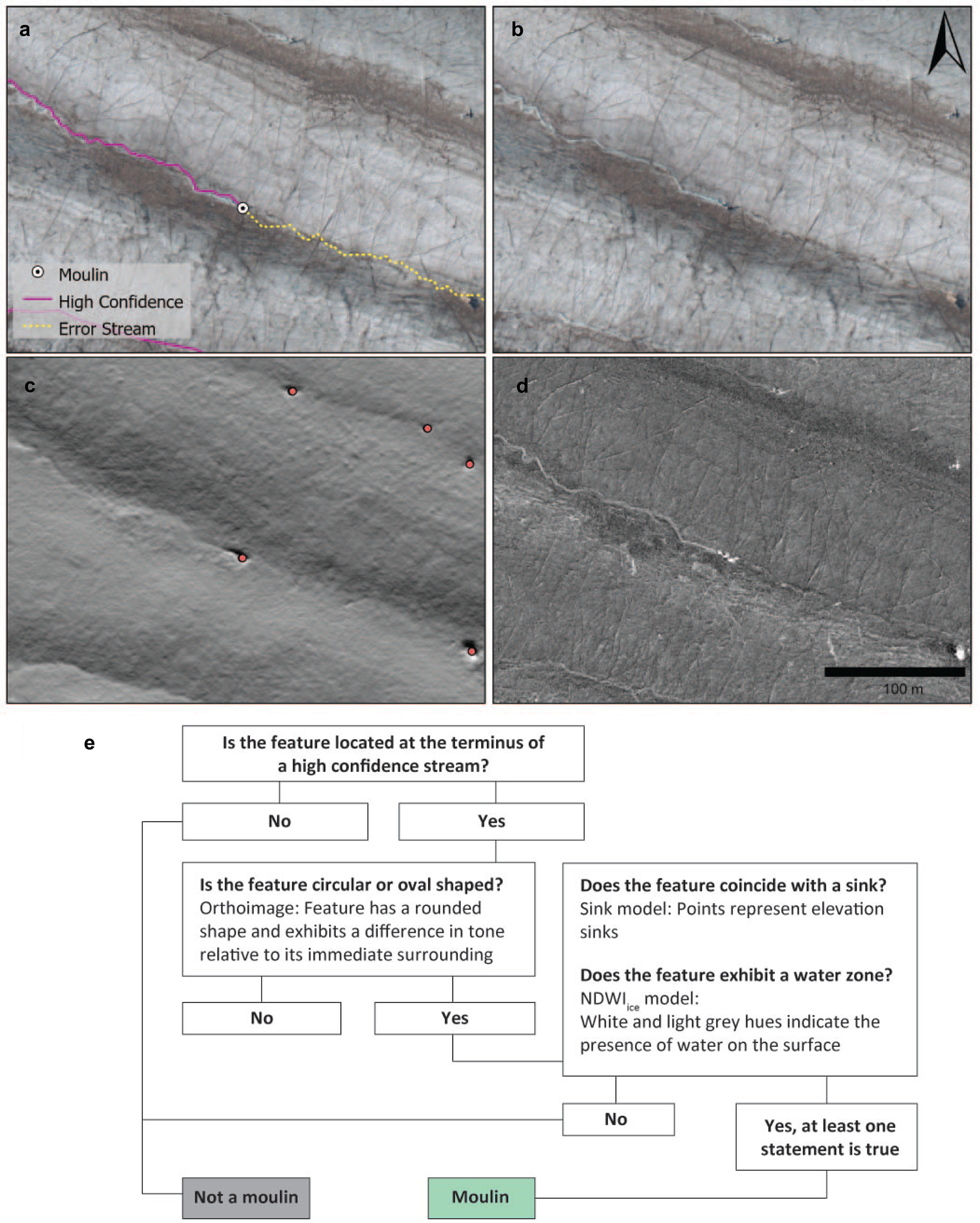
An example from Nàłùdäy of (a) delineated high-confidence and error streams, separated by a moulin, shown over the high-resolution orthmosaic (0.5 m). (b) High-resolution orthomosaic without streams delineated, illustrating that, like low-confidence streams, error streams are not linear and smooth in shape, do not exhibit white or blue tone; a change in tone is evident at the location of the moulin; (c) Hillshade model, showing no brightness consistent with a depression at the error stream location; an elevation sink (pink dots) and depression are seen at the moulin location; (d) NDWIice model, showing no light tone relative to the surroundings at the error stream location, with a bright spot at the moulin location. (E) The process of classifying moulins visualized in a flowchart.
4.3 Crevasses
Although crevasses are common features across most glaciers, we aim to identify crevasses which transfer water in this framework. These hydrologically connected crevasses serve as conduits for water to move on the surface when they become part of the stream network or have the potential to transmit water to the glacier bed. We classify these hydrologically-significant crevasses into two classes – water-filled crevasses and water-free crevasses (Fig. 6). Water-free crevasses which intersect streams have the potential to store or drain water, and often serve as initiation points for moulins, and thus we consider them hydrologically significant.
An example from Nàłùdäy of (a) delineated streams and crevasses shown over the high-resolution orthmosaic (0.5 m). (b) High-resolution orthomosaic without streams delineated, illustrating that water-filled and water-free crevasses follow or intersect stream segments, are linear and are oriented perpendicular to ice flow in the same direction as neighbouring crevasses identified in aerial imagery. (c) Water-free crevasses also coincide with sinks (pink circles, shown here over the hillshade model). (d) Water-filled crevasses show a lighter tone than their surroundings in the NDWIice. (e) The process of classifying crevasses visualized in a flowchart.
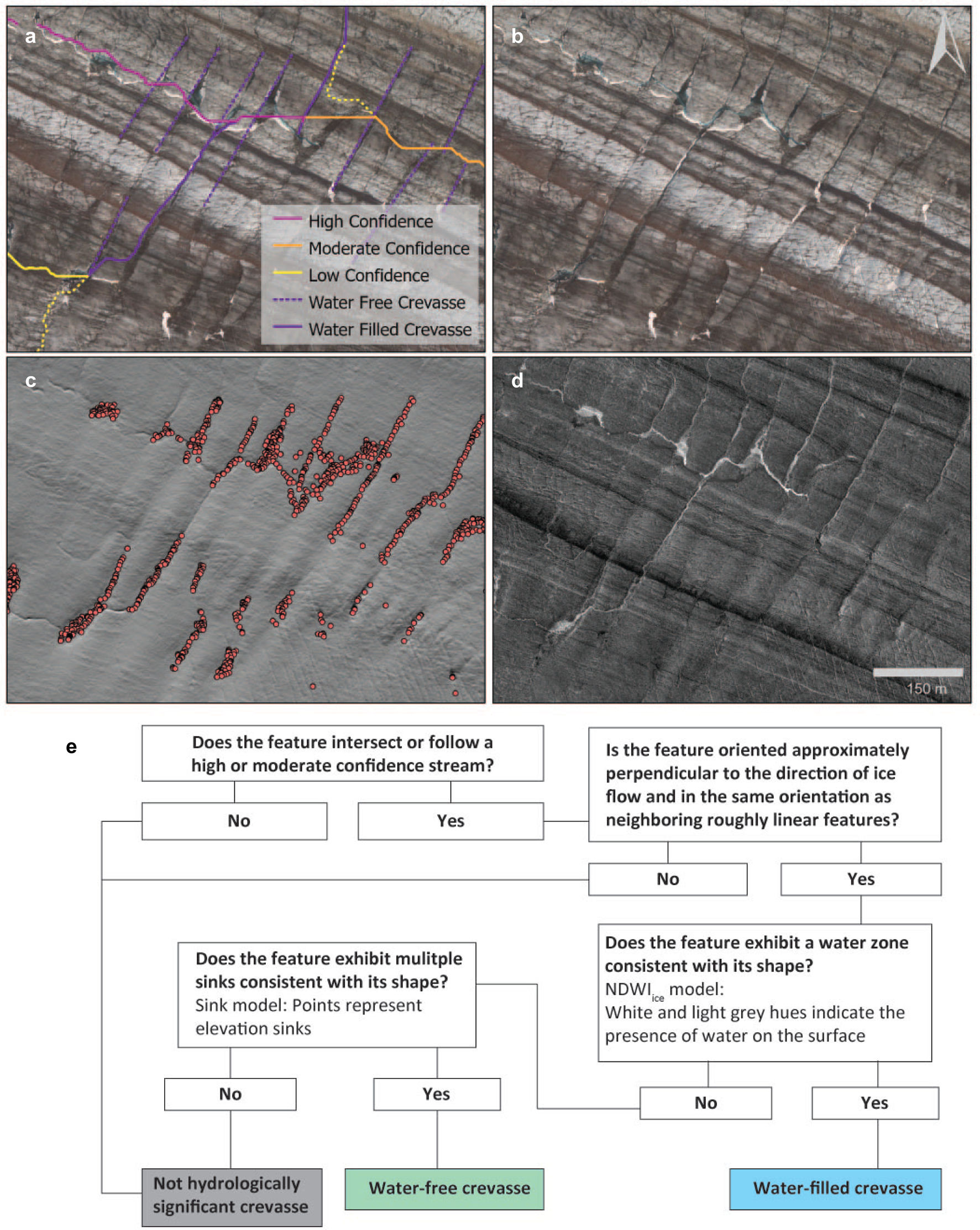
We define crevasses as features oriented approximately perpendicular to the flow direction, appearing in parallel with similar features. If the crevasse indicates a water zone in the NDWIice raster, it is classified as a water-filled crevasse. If it does not show the presence of water, but does exhibit multiple sinks consistent with its shape, it is classified as a water-free crevasse.
4.4 Ice cauldrons
An ice cauldron is a depression in the surface of a glacier, typically formed by melting of ice under the feature (Jarosch and Gudmundsson, Reference Jarosch and Gudmundsson2007; Egli and others, Reference Egli, Belotti, Ouvry, Irving and Lane2021) (see in Supplementary Appendix B figure). There are several of these on Nàłùdäy and we include them here as they provide an important connection between the supraglacial and subglacial hydrologic systems. Ice cauldrons were defined as exhibiting a circular brightness consistent with a depression (hillshade model); exhibiting a pattern of curved concentric lines (crevasses) surrounding its perimeter (aerial imagery, hillshade model); and the feature is located at the terminus of a high-confidence stream.
5. Results
5.1 Nàłùdäy – high resolution
The framework was applied over the ablation zone of Nàłùdäy (106 km2), where the surface is snow free (Figs 7a, b). We excluded snow-covered areas because they do not offer enough contrast to calculate the NDWIice and because snow-filled streams and crevasses cannot be identified in the DTM. An additional complication in applying the framework occurs in areas which are heavily crevassed. In these zones continuous streams are rarely identified in the stream model and are difficult to verify visually if they even exist. We used stream continuity to identify the limits of applying the framework in crevassed zones, in excluded areas the stream model shows long straight segments overtop of obvious crevasses and with few segments showing realistic morphology. For this reason, the lower 4 km of the ablation zone was excluded from our analysis. All classification of polylines and identification of other features was performed at a scale of 1:3000, which allowed clear differentiation of tones and textures in imagery, while also allowing for viewing of multiple stream segments at once to speed up classification.
(a) Overview of streams, moulins, crevasses and ice cauldrons at Nàłùdäy, classified with high-resolution imagery and DTM. The white dashed line indicates the extent for (b) and (c). More streams were identified using high-resolution (0.5 m) aerial imagery and DTM (B), than those identified using Sentinel-2 imagery in combination with ArcticDEM (c).
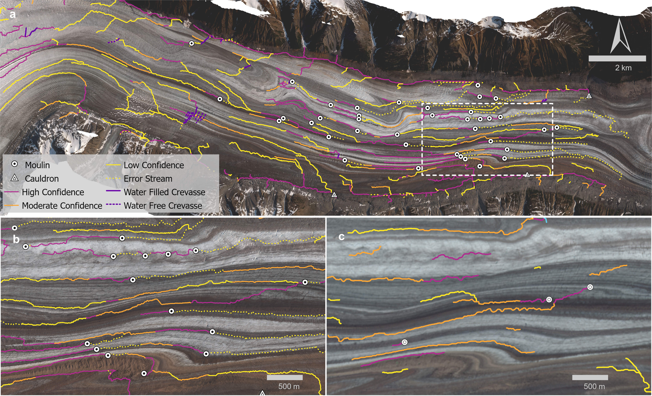
With the stream model we identified 643 km of streams at Nàłùdäy. Using the framework described above, 179 km of high-confidence streams were identified, while 50 km of streams were moderate confidence. Another 51 km of the stream model line segments were identified as error streams (where streams continued downstream of a moulin). Thirty-eight moulins were identified, 21 of which occur in the lower 4–9 km of the ablation zone (Fig. 7a).
5.2 Framework assessment
To assess the accuracy of the map produced from the framework, we manually digitized streams in a 12 km2 area of Nàłùdäy using the high-resolution data (Fig. 8). We used the definition of high-confidence streams, moulins and crevasses to identify features, leaving out moderate- and low-confidence streams. All digitizing was performed at a scale of 1:3000, to match the framework application.
Manually digitized high confidence streams, moulins and cauldrons, overlaying features identified using the framework. The region shown is the same as Figures 7b, c.
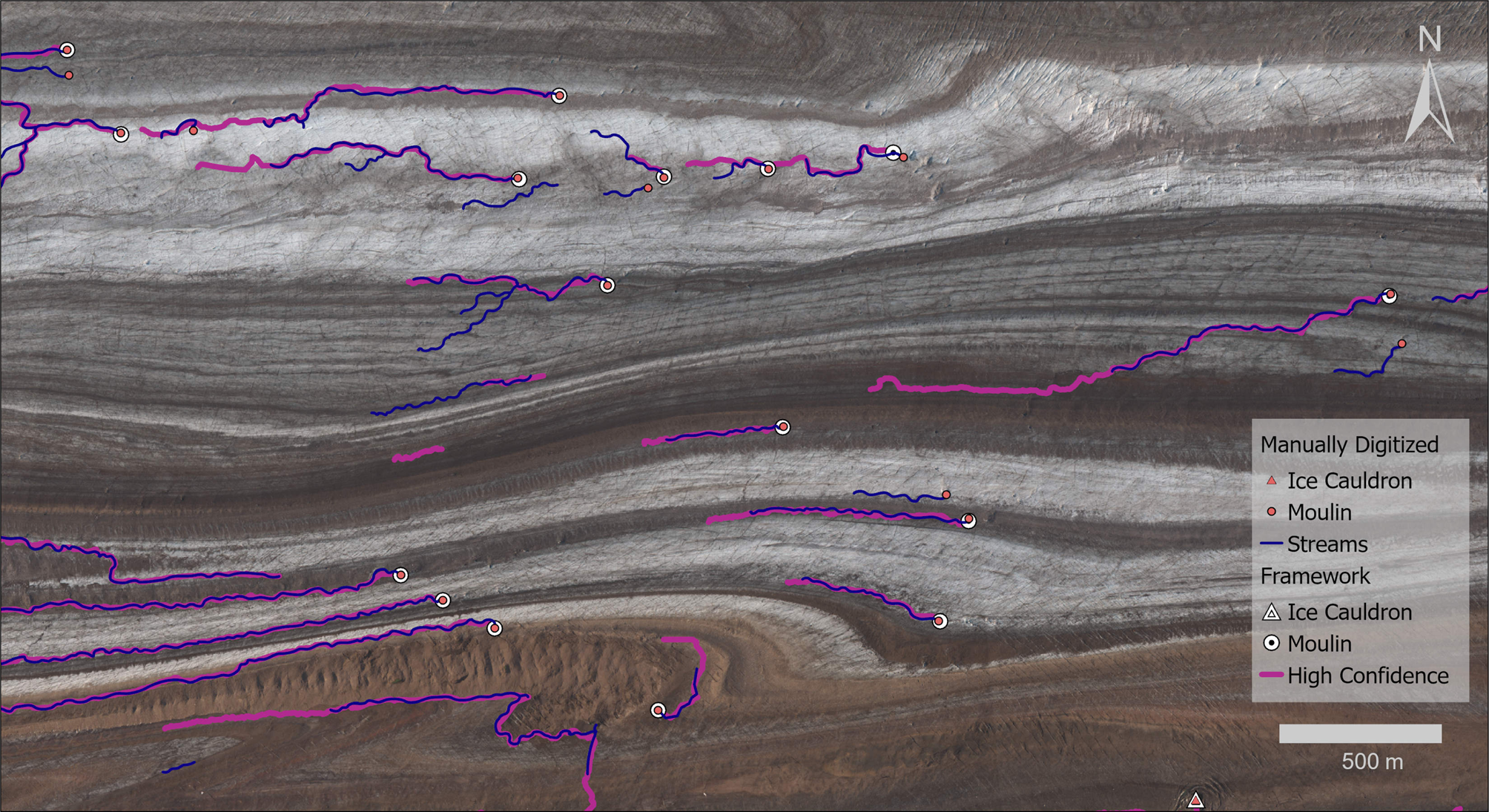
In total 19.2 km of stream were manually digitized, while 22.5 km were classified in the framework. We classified errors in the framework map into three categories: errors of omission, where high confidence streams are missing where they were manually digitized; errors of commission, where high confidence streams are present in the framework that are not present in the manual digitization; pathway errors, where both the methods have a line in the same location but pathways differ.
In total 3.4 km of stream were errors of omission, while 6.6 km were errors of commission. Almost half of the framework stream distance had pathway errors (9 km), where the stream model line segments differed from the manually digitized lines by more than 5 m. Discrepancies in these cases never exceeded 25 m, however. Errors of omission lead to identification of four additional moulins in the manually digitized data, while one additional moulin was identified in the manual dataset due to an error of commission.
5.3 Nàłùdäy – low resolution
The framework was applied to the same region of Nàłùdäy using ArcticDEM and Sentinel-2 imagery, as described above (Fig. 7c). In this test, 114 km of potential streams were identified in the low-resolution stream model (compared to 643 km in the high-resolution data). With fewer streams in the initial model, a greater proportion of stream segments were classified as high and moderate confidence (57% compared to 36%).
We found that the 10 m resolution Sentinel-2 imagery was too coarse to provide much support for stream classification, while the hillshade and NDWIice layers were more useful. Similarly, identification of moulins was challenging due to the lower resolution of the data in this test. Only eight moulins were identified using the low-resolution data, compared to 38 in the high-resolution data.
5.4 Thores Glacier
The framework was also applied to Thores Glacier, using a high-resolution (1 m) orthomosaic and DTM. Only the lower 5 km of the glacier were mapped, above that imagery is missing for the sides of the glacier making the stream model difficult to produce. A single moulin and 93 km of moderate and high confidence streams were classified (Fig. 9). The high and moderate confidence streams made up 75% of all the stream segments in the stream model.
(a) Thores Glacier with extent of inset panels shown. (b) Classified streams and moulins for study area. (c) Hillshade and (d) NDWIice for Thores study area.
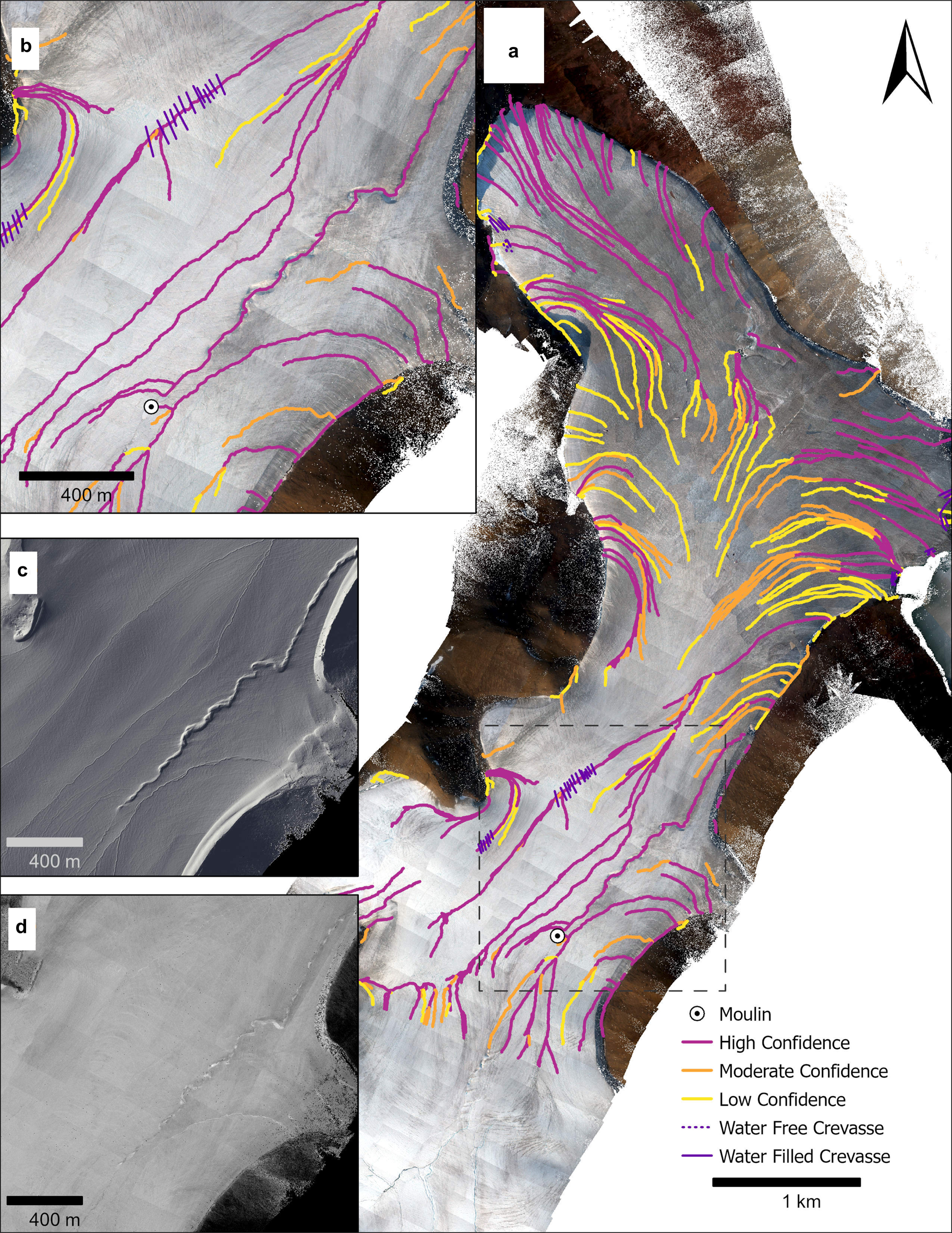
The imagery of Thores Glacier has high variability in image brightness, with some images significantly darker than others (Figs 9a, b). This can result from camera settings or changing cloud cover during a flight (Bash and others, Reference Bash, Moorman, Menounos and Gunther2020). However, by using the average RGB value to normalize the index before use in the framework, we were able to reduce the impact on NDWIice. This did not completely remove broad variations in the index (Fig. 9c), but by removing local brightness effects the NDWIice values are useful relative to surrounding pixels for identifying water on the glacier surface.
6. Discussion
The framework allows for the classification of modelled streams on a glacier by non-experts, and additionally provides clear structure for identifying moulins, crevasses and ice cauldrons connected to the drainage network. Without this framework providing clear definitions that can be applied by a wide variety of users, an expert in glacier image interpretation would need to interpret the 106 km2 of imagery at Nàłùdäy, a time-consuming task.
Nàłùdäy and Thores Glaciers present a good opportunity for testing the framework in different settings. Their distinct climate setting (sub-Arctic and high Arctic, respectively) results in marked differences in annual ablation rates, with consequent differences in hydrologic conditions. Although measuring ablation rates is outside the scope of the present study, previous work has shown recent annual melt rates of 2.31 and 1.01 m w. eq. at Nàłùdäy and Thores, respectively (Noël and others, Reference Noël2018; Hill and others, Reference Hill, Dow, Bash and Copland2021). Nàłùdäy has a lower density of streams than Thores; we identified 2.5 km−2 of high- or moderate-confidence streams in the study area of Nàłùdäy and 7.3 km−2 of high- and moderate-confidence streams in the Thores study area. The average surface slope in the lower 26 km of Nàłùdäy is 2.5%, while the slope of Thores is 6.3% for the lower 7 km where we have a DTM available. The combination of lower slope and lower stream density, coupled with warmer temperatures found in the sub-Arctic suggests that streams at Nàłùdäy are carrying greater volumes of water than those on Thores.
The large number of moulins at Nàłùdäy also suggests the subglacial hydrology is better developed than that of Thores. In addition to melt water volume, the difference in number of moulins could also be due to the contrasting strain regimes of these glaciers. As a surge-type glacier, Nàłùdäy will likely have more crevasses; this leads to more possible crevasses that can be hydrofractured to form moulins. In fact, field visits to Thores have shown no indication of moulins and the misidentified feature is likely a snowbridge with no connection to the bed, which highlights the potential for misclassification of some image features when applying the framework. Snow is a complicating factor in mapping surface hydrology on glaciers by any method. When using a DTM snow masks the stream bed, leading to streams routed elsewhere in the model, while snowbridges also mask water which may be flowing underneath, confounding automated methods based on NDWI.
6.1 Limitations of the framework
The lack of ground truth is a limitation of this framework, as with other mapping or classification schemes for supraglacial hydrology. We hope that the clearly defined characteristics of features laid out in this framework can aid in producing more accurate maps for assessing different methods, including this semi-automated approach.
In our assessment based on manually digitized features, we found 6.6 km of high confidence streams were mapped where no streams were manually digitized (errors of commission). In all but one case, these errors appear as extensions of streams beyond the ends of manually digitized streams, rather than being found in completely different locations. These errors are the result of variations in confidence across a line segment; to minimize effort very little line editing was performed during classification, except to split segments at obvious transitions.
Pathway errors are also related to the limited editing of lines, in many cases the stream model line segments may not align with visually identifiable stream centrelines, while users are likely to pick a centreline directly. This mismatch could be related to DTM errors, which will significantly impact flow accumulation calculations if present, or situations where streams are filled with water resulting in flat surfaces in the DTM. We expect these situations to have a smaller impact on the final maps produced using this framework, because stream segments are likely to still flow near their true locations.
The errors of omission are a result of the selection of the threshold value for classifying the flow accumulation raster in producing the stream model (an example of this can be seen in the upper left corner of Fig. 11). These segments have upstream catchments below the threshold, so they aren't contained in the stream model to begin with. The selection of this threshold value has been discussed in previous studies (e.g. King and others, Reference King, Hassan, Yang and Flowers2016) and stream networks are sensitive to the value chosen. King and others (Reference King, Hassan, Yang and Flowers2016) explore a range of threshold values, from 0.01 to 1.8 km2, calculated from other datasets. They found that channel densities increased by an order of magnitude between the largest and smallest of these threshold values. To avoid using visual interpretation to choose the threshold value (which leads to a circular problem of interpreting the data first) we derived an empirical threshold value using data quantiles. This derived value isolates a break in the distribution of the flow accumulation values that still captures most of the variability in the values.
Whether these errors pose a significant problem in future applications of the framework will depend on context; in the case of Thores a simple assessment by someone familiar with the site identified the problem of a misidentified moulin. Misidentification of moulins at Nàłùdäy may be harder to recognize given the number of moulins, but may also have lower impact overall if it is not widespread. In the future, additional contextual information could be taken into account in a more complex iteration of the framework, particularly in the vicinity of moulins, such as indications of stream continuation below the feature not captured by current definitions. This additional information could help identify abandoned features in addition to erroneous classifications.
6.2 Transferability of the framework
Using the framework, we were able to identify surface hydrology features on two glaciers with different morphologies. This suggests that the definitions within the framework are transferable to different settings and can provide insights into glacier surface hydrology in detail. Rather than exhaustively searching for all surface features, this framework focuses on those which are hydrologically connected, which is an efficient way to reduce the time required for creating this type of data.
These two glaciers we have applied the framework to do not represent the full breadth of conditions where supraglacial hydrology may be of interest. At the time of writing, there is significant attention being given to stability of ice shelves and the processes contributing to ice shelf dynamics (e.g. Bell and others, Reference Bell2017; Pitcher and Smith, Reference Pitcher and Smith2019). In these environments extremely low surface slopes produce different hydrological systems, where snow can act as an aquifer and slush zones are abundant (Bell and others, Reference Bell2017, Reference Bell, Banwell, Trusel and Kingslake2018). This framework has not addressed slush zones or sheet flow, but complements existing automated method for identifying these broader saturated zones. Similarly, given the large body of literature on automated lake detection through depression modelling and NDWIice methods (e.g. Arnold, Reference Arnold2010; Yang and Smith, Reference Yang and Smith2013), we have not explicitly included lakes in the development of this framework. Both slush zones and lakes can be integrated with stream networks mapped using this framework, with the framework stream segments providing inflow and outlet information about these zones. Additionally, the use of the DTM in situations where flow directions may be ambiguous has been shown to be valuable in previous work (King and others, Reference King, Hassan, Yang and Flowers2016).
The use of a DTM in determining flow pathways may also be beneficial on ice surfaces with variable albedo. The use of NDWIice has been found to perform poorly where ice surfaces are darker (Decaux and others, Reference Decaux, Grabiec, Ignatiuk and Jania2019). Our own exploration of this method did not yield good results with aerial survey data, even with the correction we applied. Further exploration of adapting this automated method to alpine glacier environments where ice surfaces have more debris, and adapting the method to imagery from commercial cameras would be of great use in the future.
6.3 Implications of data resolution
When applying the framework using lower resolution ArcticDEM and Sentinel-2 data at Nàłùdäy, fewer streams were identified in the stream model, classifying high and moderate confidence streams was more challenging, and moulin identification was limited (Fig. 10). This was due to several factors, including smoothing of the surface at lower resolution, difficulty distinguishing tone and contrast at lower resolution, and the size of features we were attempting to identify. In the high-resolution aerial imagery, high confidence streams were 5–10 pixels wide in many cases (including the stream banks which are useful in identification), which is ~2.5–5 m. In the ArcticDEM this is ~1–2 pixels wide, and less than one pixel in the Sentinel-2 imagery. Confidently identifying streams that are only 1-2 pixels wide is inherently more challenging but is further complicated by the smoothing effects of lower resolution DTMs and images where one pixel is less likely to represent a single feature (i.e. a stream may be in only a portion of a pixel; Hengl, Reference Hengl2006). This smoothing reduces changes in contrast and tone in imagery and NDWIice layers.
Stream length in each stream class as a percentage of the total stream length for both high- and low-resolution cases at Nàłùdäy. Data labels show the total length in the class.
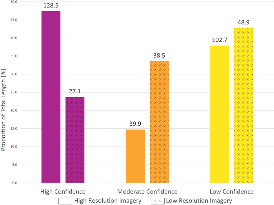
In the lower resolution DTM, smoothing from larger pixels leads to fewer streams identified in the stream model, and subsequently fewer verified streams (Fig. 10). However, the largest streams were still classified with high confidence, at both high and low resolution (Fig. 7. These larger streams are more likely to be persistent from year-to-year and thus it is smaller and less persistent streams which are likely missed in this framework (similar to King and others, Reference King, Hassan, Yang and Flowers2016). The importance of these more transient streams will shift with research objectives but should be considered when applying this framework in the future. For example, when considering hydrological catchments of moulins, stream locations and numbers may be less important than if stream locations were being used as verification of surface water routing models.
High confidence streams identified in the high- and low-resolution imagery of Nàłùdäy were not directly aligned. This may be a result of differences in coregistration of the two DTMs, which would lead to offsets in stream locations. It is also possible that, due to the time difference of 1 year or more between the acquisition of the two datasets, real migration of streams is being captured. When Nàłùdäy is not surging, it flows 0.1–1 m d−1 (Bevington and Copland, Reference Bevington and Copland2014), or 100–2000 m in the 3–6 year gap between acquisition of the low- and high-resolution datasets. Dynamic adjustments due to underlying topography can alter surface slopes and affect supraglacial drainage patterns.
Given these discrepancies and limitations related to the resolution of both the DTM and imagery used, it is important to select data with resolution appropriate to the application. For studies involving alpine glaciers, where streams are generally smaller in width, higher resolution data will allow for better identification of possible stream locations. As mentioned above, identifying features that are only 1–2 pixels wide is challenging (Hengl, Reference Hengl2006). Hengl (Reference Hengl2006) suggests that the minimum size of a resolvable object in an image is 2 × 2 pixels, suggesting that with 0.5 m resolution data streams or moulins must be a minimum of 1 m wide for identification. With 10 m resolution Sentinel-2 imagery, only streams or moulins >20 m wide will be readily identified. This inability to identify narrow stream segments could be a critical problem for quantifying changes in drainage networks, or identifying connections between the supra- and subglacial drainage systems. For studies of glaciers with larger streams or where identification of the largest streams is sufficient, lower resolution data may be adequate.
The summer acquisition for imagery and DTMs has important implications for applying this framework. Snow cover on the surface at the time of data acquisition masks surface depressions, reducing the number of streams in the stream model if early or late season data are used. In addition, late or early season imagery will have less water present on the glacier surface, affecting the calculation of NDWIice. Mismatches between the acquisition dates of the imagery and DTM will also affect feature classification, particularly in streams with less well-defined banks where NDWIice plays an important role in classification.
This framework uses a spectral index, NDWIice, which is typically calculated from reflectance data. Although digital cameras do not directly record reflectance, the increased use of structure-from-motion in various research disciplines has led to the use of imagery from consumer cameras for calculating spectral indices (e.g. Torres-Sánchez and others, Reference Torres-Sánchez, Peã, de Castro and López-Granados2014; Poley and others, Reference Poley, Laskin and McDermid2020). Unlike true reflectance data, the digital signature of consumer cameras is affected by differences in camera settings and lighting conditions. This is illustrated clearly in the Thores Glacier orthomosaic (Fig. 9), where the brightness varies significantly across the scene. We use the average value of each pixel to correct NDWIice for this bias, but more work is needed to determine if this is the best approach.
This framework is an important step in standardizing manual digitization of supraglacial hydrology for use in future studies. Models of subglacial hydrology rely on moulin locations and volume inputs as water inputs to the subglacial system (e.g. Koziol and Arnold, Reference Koziol and Arnold2018). Mapping these features systematically not only provides important boundary conditions for these models, but also provides an opportunity for examining how inputs vary over time as moulins may change in location or activity with shifting drainage networks. Investigations of supraglacial drainage and surface runoff on seasonal timescales also rely on drainage network maps (e.g. Yang and others, Reference Yang2021) and this method will add to the tools available for these studies. Supraglacial hydrology is highly dynamic (Pitcher and Smith, Reference Pitcher and Smith2019) and using this framework in conjunction with high-resolution, on-demand aerial imagery (such as is available from remotely piloted or piloted flights) will allow for detailed analysis of evolving drainage patterns. These insights can inform models of supraglacial drainage (e.g. Gleason and others, Reference Gleason2021), as well as drainage patterns in dynamics models where hydrology can impact sliding rates and ice temperatures (Sommers and Rajaram, Reference Sommers and Rajaram2020).
7. Conclusions
The image-interpretation framework for mapping supraglacial hydrological features that we present is an important step in standardization and transparency in mapping methodologies. With this framework, cross-study comparisons can be made between mapped hydrology, which is difficult to do when methods differ between studies. This framework also provides a clear method which can be implemented by non-experts, allowing for efficient data creation for further analysis.
We found that the framework was readily applied on both Nàłùdäy and Thores Glaciers, which have different surface morphologies (e.g. slope, crevassing, moraines) and climate settings. Using the framework with high-resolution imagery and DTMs, we were able to classify modelled stream segments and identify moulins, as well as hydrologically connected crevasses. Applying the framework with low-resolution data produced fewer stream segments overall but was able to capture the largest persistent streams at Nàłùdäy.
In future applications of this framework, it will be important to consider the needs of a particular study when selecting the resolution of input data and the timing of imagery and DTM acquisition. Lower resolution data are often more readily available, but in this study failed to adequately capture moulins and led to fewer stream segments compared to high-resolution data. Regardless of data resolution, the availability of mapped hydrological features provides pathways for investigating many questions relating to supraglacial hydrology and the dynamic response of glaciers to changes in hydrology.
Acknowledgements
E.A.B. was supported by a Natural Sciences and Engineering Research Council of Canada Postdoctoral Fellowship. C.S. was supported by a Natural Sciences and Engineering Research Council (NSERC) Undergraduate Student Research Award and an NSERC Discovery Grant held by G.M. C.F.D. was supported by the Natural Sciences and Engineering Research Council of Canada (NSERC 699 RGPIN-03761-2017) and the Canada Research Chairs Program (CRC 950-231237). W.K. was support by a Vanier fellowship from the Natural Sciences and Engineering Research Council. L.C. and D.M. were supported by the Natural Sciences and Engineering Research Council of Canada Discovery and Northern Supplement Programs, and the University of Ottawa through their University Research Chair program. We thank the Polar Continental Shelf Program, Kluane Lake Research Station, Parks Canada, Icefield Discovery, Warwick Vincent and Alex Culley for field support enabling aerial surveys of the sites. We thank the Nunavut Research Institute and communities of Resolute Bay and Grise Fiord for permission to undertake the fieldwork at Thores Glacier. The Yukon portion of this work was undertaken in the traditional territory of the Champagne and Aishihik First Nations, and the authors are grateful for their permission to undertake this research. Permission to use the traditional Dákwangè (Southern Tutchone) toponym for Lowell Glacier, Nàłùdäy, also spelled Nałudi, provided by Champagne and Aishihik First Nations and the Kluane First Nation. We thank both anonymous reviewers for their constructive input which greatly improved this manuscript.
Author contributions
This study was conceptualized by E.A.B., C.F.D., G.M. and C.S. C.S. developed the framework in collaboration with E.A.B., and guidance from G.M. and C.F.D. The manuscript was written by E.A.B. and C.S. C.F.D. and L.C. provided the equipment and permits for collection of aerial imagery. D.M. and W. K. designed and processed aerial survey data. All authors provided feedback on the manuscript.
Supplementary material
The supplementary material for this article can be found at https://doi.org/10.1017/jog.2022.92


 Open access