


1. Introduction
We consider cyclic unramified coverings of degree d of irreducible complex smooth genus-
 $2$
curves and their corresponding Prym varieties. They provide natural examples of polarized abelian varieties with automorphisms of order d. The rich geometry of the associated Prym map has been studied in several papers; see [Reference Agostini1, Reference Albano and Pirola2, Reference Lange and Ortega7, Reference Lange and Ortega8, Reference Ortega11, Reference Ries13], among others. Notice that the classical case,
$2$
curves and their corresponding Prym varieties. They provide natural examples of polarized abelian varieties with automorphisms of order d. The rich geometry of the associated Prym map has been studied in several papers; see [Reference Agostini1, Reference Albano and Pirola2, Reference Lange and Ortega7, Reference Lange and Ortega8, Reference Ortega11, Reference Ries13], among others. Notice that the classical case,
 $d=2$
, is completely explained in [Reference Mumford9, section 7] and [Reference Naranjo10]. Nevertheless, very little is known for higher values of d. In this article, we investigate whether the covering can be reconstructed from its Prym variety, that is, whether the generic Prym Torelli theorem holds for these coverings.
$d=2$
, is completely explained in [Reference Mumford9, section 7] and [Reference Naranjo10]. Nevertheless, very little is known for higher values of d. In this article, we investigate whether the covering can be reconstructed from its Prym variety, that is, whether the generic Prym Torelli theorem holds for these coverings.
It is known that the Prym variety of an unramified cyclic covering (over any smooth curve) is isomorphic, as unpolarized varieties, to the product of two Jacobians (see [Reference Ortega11]), and when the degree d is odd, the Jacobians are isomorphic. Moreover, when d is not prime, the existence of intermediate coverings gives a much more complicated scenario, which strongly depends on the decomposition of d in primes. For this reason, as in [Reference Ries13], we assume d to be an odd prime.
Putting this in a modular setting, we consider the moduli spaceFootnote
1
 $\mathcal R^d$
of isomorphism classes of cyclic unramified coverings
$\mathcal R^d$
of isomorphism classes of cyclic unramified coverings
 $f:\widetilde C\rightarrow C$
, with
$f:\widetilde C\rightarrow C$
, with
 $g(C)=2$
and
$g(C)=2$
and
 $\deg (f)=d$
. Equivalently,
$\deg (f)=d$
. Equivalently,
 $\mathcal R^d$
parametrizes isomorphism classes of pairs
$\mathcal R^d$
parametrizes isomorphism classes of pairs
 $(C,\langle \eta \rangle )$
, where
$(C,\langle \eta \rangle )$
, where
 $\eta $
is a d-torsion point in
$\eta $
is a d-torsion point in
 $JC$
generating a subgroup
$JC$
generating a subgroup
 $\langle \eta \rangle \cong \mathbb Z/d\mathbb Z$
. We recall that the curve
$\langle \eta \rangle \cong \mathbb Z/d\mathbb Z$
. We recall that the curve
 $\widetilde C$
is constructed by applying the
$\widetilde C$
is constructed by applying the
 $\mathrm {Spec}$
functor to the sheaf of
$\mathrm {Spec}$
functor to the sheaf of
 $\mathcal O_{C}$
-algebras:
$\mathcal O_{C}$
-algebras:
 $$\begin{align*}\mathcal O_C \oplus \eta \oplus \eta^2 \oplus \ldots \eta^{d-1}. \end{align*}$$
Notice that
 $\widetilde C$
comes equipped with an automorphism
$\widetilde C$
comes equipped with an automorphism
 $\sigma $
of order d such that
$\sigma $
of order d such that
 $C=\widetilde C/\langle \sigma \rangle $
.
$C=\widetilde C/\langle \sigma \rangle $
.
An important consequence of this construction is that it shows that any automorphism of C leaving
 $\langle \eta \rangle $
invariant lifts to an automorphism on
$\langle \eta \rangle $
invariant lifts to an automorphism on
 $\widetilde C$
. This is the case of the hyperelliptic involution on C, which lifts to an involution j on
$\widetilde C$
. This is the case of the hyperelliptic involution on C, which lifts to an involution j on
 $\widetilde C$
. Therefore, the dihedral group generated by
$\widetilde C$
. Therefore, the dihedral group generated by
 $\sigma $
and j acts on
$\sigma $
and j acts on
 $\widetilde C$
providing an interesting geometric structure in the several Jacobians and Pryms appearing naturally in the picture. We focus on the Prym variety
$\widetilde C$
providing an interesting geometric structure in the several Jacobians and Pryms appearing naturally in the picture. We focus on the Prym variety
 $P(\widetilde C,C)$
defined as the component of the origin of the kernel of the norm map
$P(\widetilde C,C)$
defined as the component of the origin of the kernel of the norm map
 $J\widetilde C\rightarrow JC.$
It is a consequence of the Riemann–Hurwitz theorem that
$J\widetilde C\rightarrow JC.$
It is a consequence of the Riemann–Hurwitz theorem that
 $g(\widetilde C)=d+1$
, and thus
$g(\widetilde C)=d+1$
, and thus
 $\dim P(\widetilde C,C)=d-1$
. Moreover, the principal polarization on
$\dim P(\widetilde C,C)=d-1$
. Moreover, the principal polarization on
 $J\widetilde C$
induces on
$J\widetilde C$
induces on
 $P(\widetilde C,C)$
a polarization
$P(\widetilde C,C)$
a polarization
 $\tau $
of type
$\tau $
of type
 $(1,\ldots ,1,d)$
. We can define the Prym map as the map of moduli stacks:
$(1,\ldots ,1,d)$
. We can define the Prym map as the map of moduli stacks:
 $$\begin{align*}{\mathcal P}_d:{\mathcal R}^{d} \longrightarrow {\mathcal A}_{d-1}^{(1,\ldots,1,d)}, \end{align*}$$
which maps
 $f:\widetilde C\rightarrow C$
to the isomorphism class of
$f:\widetilde C\rightarrow C$
to the isomorphism class of
 $(P(\widetilde C,C), \tau )$
.
$(P(\widetilde C,C), \tau )$
.
It is known that the generic fiber of
 ${\mathcal P}_d$
is positive dimensional for
${\mathcal P}_d$
is positive dimensional for
 $d=3,5$
([Reference Albano and Pirola2]), for
$d=3,5$
([Reference Albano and Pirola2]), for
 $d=7$
the degree onto its image is
$d=7$
the degree onto its image is
 $10$
([Reference Lange and Ortega8]) and the map is generically finite for
$10$
([Reference Lange and Ortega8]) and the map is generically finite for
 $d\ge 7$
([Reference Agostini1]). In this paper, we prove:
$d\ge 7$
([Reference Agostini1]). In this paper, we prove:
Theorem 1.1. The Prym map
 $\mathcal P_d$
is generically injective for every prime
$\mathcal P_d$
is generically injective for every prime
 $d\ge 11$
such that
$d\ge 11$
such that
 $k:=\frac {d-1}2$
is also prime.
$k:=\frac {d-1}2$
is also prime.
Remark 1.2. It is conjectured that there are infinitely many pairs of prime numbers of the form
 $(k,2k+1)$
. These are called Sophie Germain prime numbers. Under this hypothesis on d and k, we will say that
$(k,2k+1)$
. These are called Sophie Germain prime numbers. Under this hypothesis on d and k, we will say that
 $f: \widetilde C \rightarrow C$
is of Sophie Germain type.
$f: \widetilde C \rightarrow C$
is of Sophie Germain type.
Our proof has ingredients of different nature. We use arithmetic arguments on abelian varieties of
 $GL_2$
-type to analyze the endomorphism algebra of some Jacobians, combined with the use of theta-duality techniques inspired by the Fourier–Mukai transform.
$GL_2$
-type to analyze the endomorphism algebra of some Jacobians, combined with the use of theta-duality techniques inspired by the Fourier–Mukai transform.
More precisely: The automorphism
 $\sigma $
on
$\sigma $
on
 $\widetilde C$
induces an automorphism, denoted by the same letter, on
$\widetilde C$
induces an automorphism, denoted by the same letter, on
 $P:=P(\widetilde C,C)$
preserving the polarization
$P:=P(\widetilde C,C)$
preserving the polarization
 $\tau $
and fixing point-wise the kernel of
$\tau $
and fixing point-wise the kernel of
 $\lambda _{\tau }:P\rightarrow P^{\vee }$
. We prove first that
$\lambda _{\tau }:P\rightarrow P^{\vee }$
. We prove first that
 $\sigma $
is, generically, completely determined by
$\sigma $
is, generically, completely determined by
 $(P,\tau )$
. Then, we consider the curve
$(P,\tau )$
. Then, we consider the curve
 $C_0:=\widetilde C/\langle j \rangle $
, where j is a lifting of the hyperelliptic involution on C. In the second step, using a result of arithmetic nature ([Reference Guitart5, Reference Wu15]), we prove that for a generic covering, the only automorphisms of
$C_0:=\widetilde C/\langle j \rangle $
, where j is a lifting of the hyperelliptic involution on C. In the second step, using a result of arithmetic nature ([Reference Guitart5, Reference Wu15]), we prove that for a generic covering, the only automorphisms of
 $C_0$
are the identity and, possibly, the hyperelliptic involution.
$C_0$
are the identity and, possibly, the hyperelliptic involution.
Next, we consider the isomorphisms
 $JC_0\times JC_0 \rightarrow P$
studied in [Reference Ries13] and [Reference Ortega11]. We prove, using step 2, that these isomorphisms are unique in general, which allows us to recover canonically from
$JC_0\times JC_0 \rightarrow P$
studied in [Reference Ries13] and [Reference Ortega11]. We prove, using step 2, that these isomorphisms are unique in general, which allows us to recover canonically from
 $(P,\tau )$
the curve
$(P,\tau )$
the curve
 $C_0$
and a set of automorphisms
$C_0$
and a set of automorphisms
 $\beta _i$
on
$\beta _i$
on
 $JC_0$
.
$JC_0$
.
Finally, we show how to reconstruct the covering
 $f:\widetilde C\rightarrow C$
from these data. The key argument is that the whole diagram (2.1) is determined by the map
$f:\widetilde C\rightarrow C$
from these data. The key argument is that the whole diagram (2.1) is determined by the map
 $h_0:C_0\rightarrow \mathbb P^1$
. We recover explicitly the fibers of
$h_0:C_0\rightarrow \mathbb P^1$
. We recover explicitly the fibers of
 $h_0$
in the following way: We fix a point
$h_0$
in the following way: We fix a point
 $x\in C_0$
to embed
$x\in C_0$
to embed
 $C_0$
in
$C_0$
in
 $JC_0$
, and then we compute the theta dual (as introduced in [Reference Pareschi and Popa12] and used in [Reference Lahoz and Naranjo6]) of the curves
$JC_0$
, and then we compute the theta dual (as introduced in [Reference Pareschi and Popa12] and used in [Reference Lahoz and Naranjo6]) of the curves
 $\beta _i(C_0)\subset JC_0$
. This gives a translation of the Brill–Noether locus
$\beta _i(C_0)\subset JC_0$
. This gives a translation of the Brill–Noether locus
 $W_{k-3}(C_0)$
by an effective degree
$W_{k-3}(C_0)$
by an effective degree
 $2$
divisor defined by two points in the fiber
$2$
divisor defined by two points in the fiber
 $h_0^{-1}(h_0(x))$
. Varying i, we recover the whole fiber of
$h_0^{-1}(h_0(x))$
. Varying i, we recover the whole fiber of
 $h_0$
at
$h_0$
at
 $h_0(x)$
, and this ends the proof.
$h_0(x)$
, and this ends the proof.
In the last sections of the paper, we consider the cases
 $d=9$
and
$d=9$
and
 $d=13$
, which illustrate that without our assumptions the generic injectivity requires a case-by-case analysis which depends on the decomposition of d and k in prime numbers.
$d=13$
, which illustrate that without our assumptions the generic injectivity requires a case-by-case analysis which depends on the decomposition of d and k in prime numbers.
When
 $d=9$
, since d is not prime, we have additional curves in the diagram. In this case, a deeper analysis of the automorphisms that appear in step 3 combined with Galois theory arguments allows us to conclude the following (see Theorem 4.6):
$d=9$
, since d is not prime, we have additional curves in the diagram. In this case, a deeper analysis of the automorphisms that appear in step 3 combined with Galois theory arguments allows us to conclude the following (see Theorem 4.6):
Theorem 1.3. The Prym map
 $\mathcal P_{9}$
is generically injective.
$\mathcal P_{9}$
is generically injective.
We finish by studying the case
 $d=13$
, providing a necessary condition for the generic injectivity of the Prym map
$d=13$
, providing a necessary condition for the generic injectivity of the Prym map
 $\mathcal P_{13}$
.
$\mathcal P_{13}$
.
2. Setup and notations
The content of this section is borrowed from [Reference Ries13] and [Reference Ortega11]. We will state the results of these two papers without further quoting. Let
 $f: \widetilde C \rightarrow C$
be a cyclic d-covering of a curve C of genus
$f: \widetilde C \rightarrow C$
be a cyclic d-covering of a curve C of genus
 $2$
associated to a nontrivial d-torsion point
$2$
associated to a nontrivial d-torsion point
 $\eta \in JC[d]$
. We denote by
$\eta \in JC[d]$
. We denote by
 $\sigma $
both the automorphism of order d on
$\sigma $
both the automorphism of order d on
 $\widetilde C$
and the induced automorphism on
$\widetilde C$
and the induced automorphism on
 $J\widetilde C$
. The Prym variety of the covering,
$J\widetilde C$
. The Prym variety of the covering,
 $P:=P(\widetilde C,C)$
, is the component of the origin of the kernel of the norm map. One easily checks that
$P:=P(\widetilde C,C)$
, is the component of the origin of the kernel of the norm map. One easily checks that
 $\sigma $
leaves P invariant, so we keep the notation
$\sigma $
leaves P invariant, so we keep the notation
 $\sigma $
for the restriction to P. The polarization on
$\sigma $
for the restriction to P. The polarization on
 $J\widetilde C$
induces on P a polarization
$J\widetilde C$
induces on P a polarization
 $\tau $
of type
$\tau $
of type
 $(1,\ldots ,1,d)$
which is invariant by
$(1,\ldots ,1,d)$
which is invariant by
 $\sigma $
, that is, there is a line bundle
$\sigma $
, that is, there is a line bundle
 $L\in Pic(P)$
representing
$L\in Pic(P)$
representing
 $\tau \in NS(P)$
such that
$\tau \in NS(P)$
such that
 $\sigma ^*(L)\cong L$
. Moreover, we have:
$\sigma ^*(L)\cong L$
. Moreover, we have:
Lemma 2.1. The set of fixed points of
 $\sigma $
on P is exactly the kernel
$\sigma $
on P is exactly the kernel
 $K(\tau )$
of the polarization map
$K(\tau )$
of the polarization map
 $\lambda _{\tau }:P\rightarrow P^{\vee }$
. Moreover,
$\lambda _{\tau }:P\rightarrow P^{\vee }$
. Moreover,
 $K(\tau )= P\cap f^*(JC)$
.
$K(\tau )= P\cap f^*(JC)$
.
From now on, we assume that d is an odd prime, and we set
 $d=2k+1$
.
$d=2k+1$
.
The hyperelliptic involution
 $\iota $
on C lifts to an involution j on
$\iota $
on C lifts to an involution j on
 $\widetilde C$
. The dihedral group with
$\widetilde C$
. The dihedral group with
 $2d$
elements generated by j and
$2d$
elements generated by j and
 $\sigma $
acts on
$\sigma $
acts on
 $\widetilde C$
. Notice that all the automorphisms
$\widetilde C$
. Notice that all the automorphisms
 $j\circ \sigma ^i$
are involutions on
$j\circ \sigma ^i$
are involutions on
 $\widetilde C$
lifting
$\widetilde C$
lifting
 $\iota $
. We define the following curves:
$\iota $
. We define the following curves:
 $$\begin{align*}C_0:=\widetilde C/\langle j \rangle, \quad C_1:=\widetilde C/\langle j\sigma \rangle, \quad \ldots \quad C_{d-1}:=\widetilde C/\langle j\sigma^{d-1} \rangle. \end{align*}$$
And we denote by
 $\pi _i:\widetilde C\rightarrow C_i$
,
$\pi _i:\widetilde C\rightarrow C_i$
,
 $i=0,\ldots , d-1$
the quotient maps. These curves fit in the following commutative diagram:
$i=0,\ldots , d-1$
the quotient maps. These curves fit in the following commutative diagram:

where the maps
 $\varepsilon , \pi _0,\ldots , \pi _{d-1}$
are of degree
$\varepsilon , \pi _0,\ldots , \pi _{d-1}$
are of degree
 $2$
and the maps
$2$
and the maps
 $f, h_0, h_1,\ldots ,h_{d-1}$
of degree d. Moreover, since d is odd, all the involution in the dihedral group are conjugate to each other, therefore all the curves
$f, h_0, h_1,\ldots ,h_{d-1}$
of degree d. Moreover, since d is odd, all the involution in the dihedral group are conjugate to each other, therefore all the curves
 $C_i$
are mutually isomorphic. Moreover,
$C_i$
are mutually isomorphic. Moreover,
 $g(C_0)=g(C_1)=\ldots = g(C_{d-1})=k$
. In fact, all the maps
$g(C_0)=g(C_1)=\ldots = g(C_{d-1})=k$
. In fact, all the maps
 $\pi _i$
ramify in six points, one in each preimage by f of the Weierstrass points of C. In particular,
$\pi _i$
ramify in six points, one in each preimage by f of the Weierstrass points of C. In particular,
 $\pi _i^*:JC_i \rightarrow J\widetilde C$
is injective. From now on, we identify
$\pi _i^*:JC_i \rightarrow J\widetilde C$
is injective. From now on, we identify
 $JC_i$
with its image in
$JC_i$
with its image in
 $J\widetilde C$
.
$J\widetilde C$
.
Proposition 2.2. (Ortega, Ries). With the notations in the diagram (2.1) and denoting by P the Prym variety
 $P(\widetilde C,C)$
, the following statements hold for any
$P(\widetilde C,C)$
, the following statements hold for any
 $i=0,\ldots , d-1$
:
$i=0,\ldots , d-1$
:
-
a)
 $JC_i\subset P$
.
$JC_i\subset P$
. -
b) The automorphism
$\sigma ^i$
sends
$JC_0$
to
$JC_{d-2i}$
for
$i\leq k$
, and to
$JC_{2d-2i}$
for
$i> k$
. -
c) The automorphism
$\beta _i:=\sigma ^i+\sigma ^{-i}$
leaves invariant
$JC_0$
.


A crucial ingredient for the proof of our main theorem is the existence of k isomorphisms:
 $$\begin{align*}\psi_i: JC_0 \times JC_0 \longrightarrow JC_0 \times JC_{d-2i} \longrightarrow P, \end{align*}$$
where the first map sends
 $(x,y)$
to
$(x,y)$
to
 $(x,\sigma ^i(y))$
(for
$(x,\sigma ^i(y))$
(for
 $i=1,\ldots ,k$
), and the second is the addition map.
$i=1,\ldots ,k$
), and the second is the addition map.
Let us denote by
 $\lambda _N:JN\rightarrow JN^{\vee }$
the isomorphism attached to the natural principal polarization on a smooth irreducible curve N. We will keep this notation for the rest of the paper.
$\lambda _N:JN\rightarrow JN^{\vee }$
the isomorphism attached to the natural principal polarization on a smooth irreducible curve N. We will keep this notation for the rest of the paper.
The pull-back of the polarization
 $\tau $
to
$\tau $
to
 $JC_0\times JC_0$
gives rise to the following commutative diagram:
$JC_0\times JC_0$
gives rise to the following commutative diagram:

where
 $M_i$
is the matrix
$M_i$
is the matrix
 $$\begin{align*}\left( \begin{array}{cc} 2 & \beta_i \\ \beta_i & 2 \end{array} \right), \end{align*}$$
and the automorphisms
 $\beta _i$
, for
$\beta _i$
, for
 $i=1,\ldots ,k$
of
$i=1,\ldots ,k$
of
 $JC_0$
are those appearing in the previous proposition.
$JC_0$
are those appearing in the previous proposition.
It will also be useful to know the pull-back of the automorphisms
 $\sigma ^i$
to
$\sigma ^i$
to
 $JC_0\times JC_0$
through the isomorphisms
$JC_0\times JC_0$
through the isomorphisms
 $\psi _i$
. Indeed, we have the following:
$\psi _i$
. Indeed, we have the following:
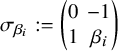
Proposition 2.3. For any
 $i=1,\ldots ,k$
we have the equality:
$i=1,\ldots ,k$
we have the equality:
 $$\begin{align*}\sigma^i \circ \psi_i= \psi_i\circ \begin{pmatrix}0 & -1\\1&\beta_i\end{pmatrix}. \end{align*}$$
Remark 2.4. Notice that a priori
 $\psi _i^*(\langle \sigma \rangle )$
yields
$\psi _i^*(\langle \sigma \rangle )$
yields
 $d-1$
automorphisms of
$d-1$
automorphisms of
 $JC_0\times JC_0$
. The crucial point is that only one among them is of type
$JC_0\times JC_0$
. The crucial point is that only one among them is of type
 $$ \begin{align*} \begin{pmatrix} 0 & *\\1 & * \end{pmatrix}. \end{align*} $$
3. Proof of the main theorem
Our aim is to prove the generic injectivity of the map
 $$\begin{align*}\mathcal P_d:\mathcal R^d \longrightarrow \mathcal A_{d-1}^{(1,\ldots,1,d)}, \end{align*}$$
with
 $d=2k+1$
, assuming k and d primes.
$d=2k+1$
, assuming k and d primes.
3.1. First step: uniqueness of
$\sigma $
.

We want to use the automorphism
 $\sigma $
in order to read from
$\sigma $
in order to read from
 $(P,\tau )$
relevant information to reconstruct
$(P,\tau )$
relevant information to reconstruct
 $(\widetilde C,C)$
. We shall show that the only automorphisms of P of order d preserving
$(\widetilde C,C)$
. We shall show that the only automorphisms of P of order d preserving
 $\tau $
and in fact, fixing point-wise
$\tau $
and in fact, fixing point-wise
 $K(\tau )$
(see Lemma 2.1) are the powers
$K(\tau )$
(see Lemma 2.1) are the powers
 $\sigma ^i $
.
$\sigma ^i $
.
Proposition 3.1. Let P be a general element in
 $Im(\mathcal {P}_d)$
. Then the group of automorphisms
$Im(\mathcal {P}_d)$
. Then the group of automorphisms
 $$ \begin{align*}\{ \epsilon \in Aut((P,\tau)) \ \mid \ \epsilon (x)=x, \ \forall x\in K(\tau) \}\end{align*} $$
is
 $\langle \sigma \rangle \simeq \mathbb Z/d\mathbb Z$
.
$\langle \sigma \rangle \simeq \mathbb Z/d\mathbb Z$
.
Proof. Let P and
 $\epsilon \neq \mathrm {Id}$
be as in the statement. We will see that
$\epsilon \neq \mathrm {Id}$
be as in the statement. We will see that
 $\epsilon =\sigma ^i$
for some
$\epsilon =\sigma ^i$
for some
 $i=1,\ldots ,d-1$
, where
$i=1,\ldots ,d-1$
, where
 $\sigma $
is as in Section 2. Due to Lemma 2.1, there is an automorphism
$\sigma $
is as in Section 2. Due to Lemma 2.1, there is an automorphism
 $\tilde \epsilon : J\widetilde C \rightarrow J\widetilde C$
such that the following diagram is commutative:
$\tilde \epsilon : J\widetilde C \rightarrow J\widetilde C$
such that the following diagram is commutative:

where
 $\mu :f^*JC \times P \rightarrow J\widetilde C$
stands for the addition map. According to the diagram,
$\mu :f^*JC \times P \rightarrow J\widetilde C$
stands for the addition map. According to the diagram,
 $\mu ^* \tilde \epsilon ^* \mathcal O_{J\widetilde C}(\widetilde \Theta )$
equals, as polarizations,
$\mu ^* \tilde \epsilon ^* \mathcal O_{J\widetilde C}(\widetilde \Theta )$
equals, as polarizations,
 $\mu ^*\mathcal O_{J\widetilde C}(\widetilde \Theta )$
. Since
$\mu ^*\mathcal O_{J\widetilde C}(\widetilde \Theta )$
. Since
 $\mu $
is an isogeny, the kernel of
$\mu $
is an isogeny, the kernel of
 $\mu ^*$
is finite and therefore
$\mu ^*$
is finite and therefore
 $$\begin{align*}\tilde \epsilon ^{\,*} \mathcal O_{J\widetilde C}(\widetilde \Theta)\otimes \mathcal O_{J\widetilde C}(-\widetilde \Theta ) \end{align*}$$
is a torsion sheaf, in particular belongs to
 $Pic^0(J\widetilde C)$
. Hence,
$Pic^0(J\widetilde C)$
. Hence,
 $\tilde \epsilon ^* \mathcal O_{J\widetilde C}(\widetilde \Theta )$
induces the canonical polarization on
$\tilde \epsilon ^* \mathcal O_{J\widetilde C}(\widetilde \Theta )$
induces the canonical polarization on
 $J\widetilde C$
, and thus, by the Torelli theorem, there is an automorphism
$J\widetilde C$
, and thus, by the Torelli theorem, there is an automorphism
 $\tilde \epsilon _0$
on
$\tilde \epsilon _0$
on
 $\widetilde C$
inducing
$\widetilde C$
inducing
 $\tilde \epsilon $
. Notice that, by construction,
$\tilde \epsilon $
. Notice that, by construction,
 $\tilde \epsilon $
is the identity on
$\tilde \epsilon $
is the identity on
 $f^*(JC)$
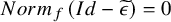
. We claim that
$f^*(JC)$
. We claim that
 $Norm_f (Id-\widetilde \epsilon )=0$
. Indeed, for all
$Norm_f (Id-\widetilde \epsilon )=0$
. Indeed, for all
 $x\in J\widetilde C$
we write
$x\in J\widetilde C$
we write
 $x=y+f^*(z)$
, where
$x=y+f^*(z)$
, where
 $y\in P$
and
$y\in P$
and
 $z\in JC$
. Then:
$z\in JC$
. Then:
 $$\begin{align*}(Id-\widetilde \epsilon )(x)=y+f^*(z)- (\widetilde \epsilon (y)+f^*(z))= y-\widetilde \epsilon (y). \end{align*}$$
Since
 $\widetilde \epsilon $
leaves invariant P, we obtain that
$\widetilde \epsilon $
leaves invariant P, we obtain that
 $Norm_f(Id-\widetilde \epsilon )=0$
. Let
$Norm_f(Id-\widetilde \epsilon )=0$
. Let
 $p_1,p_2\in \widetilde C$
be two points with
$p_1,p_2\in \widetilde C$
be two points with
 $f(p_1)=f(p_2)$
. Then the norm of
$f(p_1)=f(p_2)$
. Then the norm of
 $p_1-p_2-\widetilde \epsilon _0(p_1)+\widetilde \epsilon _0(p_2)$
is zero. This implies that
$p_1-p_2-\widetilde \epsilon _0(p_1)+\widetilde \epsilon _0(p_2)$
is zero. This implies that
 $f(\widetilde \epsilon _0(p_1))=f(\widetilde \epsilon _0(p_2))$
, hence
$f(\widetilde \epsilon _0(p_1))=f(\widetilde \epsilon _0(p_2))$
, hence
 $\tilde \epsilon _0$
descends to an automorphism of C. Since C is generic, this automorphism must be either the identity or the hyperelliptic involution. The latter it is not possible, since the hyperelliptic involution induces
$\tilde \epsilon _0$
descends to an automorphism of C. Since C is generic, this automorphism must be either the identity or the hyperelliptic involution. The latter it is not possible, since the hyperelliptic involution induces
 $-Id$
in
$-Id$
in
 $f^*(JC)$
.
$f^*(JC)$
.
So
 $\tilde \epsilon _0$
preserves the fibers of f and descends to the identity automorphism of C. Therefore,
$\tilde \epsilon _0$
preserves the fibers of f and descends to the identity automorphism of C. Therefore,
 $\tilde \epsilon _0$
belongs to the Galois group of
$\tilde \epsilon _0$
belongs to the Galois group of
 $\widetilde C$
over C which is the cyclic group generated by
$\widetilde C$
over C which is the cyclic group generated by
 $\sigma $
.
$\sigma $
.
3.2. Second step: determination of the automorphisms on
$C_0$

This subsection is devoted to the study of the possible automorphisms on
 $C_0$
that will appear in the third step. From now on, the covering
$C_0$
that will appear in the third step. From now on, the covering
 $\widetilde C\rightarrow C$
is generic in
$\widetilde C\rightarrow C$
is generic in
 $\mathcal R^d$
. Given an abelian variety A, we denote by
$\mathcal R^d$
. Given an abelian variety A, we denote by
 $End(A)$
its endomorphism ring and by
$End(A)$
its endomorphism ring and by
 $End^0(A)$
the endomorphism algebra
$End^0(A)$
the endomorphism algebra
 $End(A)\otimes _{\mathbb {Z}}\mathbb {Q}$
. Recall that a CM-field E is a number field with exactly one complex multiplication, equivalently E is a totally imaginary quadratic extension of a totally real number field. A CM-algebra is a finite product of CM-fields.
$End(A)\otimes _{\mathbb {Z}}\mathbb {Q}$
. Recall that a CM-field E is a number field with exactly one complex multiplication, equivalently E is a totally imaginary quadratic extension of a totally real number field. A CM-algebra is a finite product of CM-fields.
Definition 3.2. The abelian variety A is said to be of
 $GL_2$
-type if for some number field E such that
$GL_2$
-type if for some number field E such that
 $[E:\mathbb {Q}]=\dim A$
, there is an embedding of
$[E:\mathbb {Q}]=\dim A$
, there is an embedding of
 $\mathbb {Q}$
-algebras
$\mathbb {Q}$
-algebras
 $E\hookrightarrow End^0(A)$
.
$E\hookrightarrow End^0(A)$
.
Definition 3.3. The abelian variety A is said to be of CM-type if for some CM-field E such that
 $[E:\mathbb {Q}]=2\dim A$
, there is an embedding of
$[E:\mathbb {Q}]=2\dim A$
, there is an embedding of
 $\mathbb {Q}$
-algebras
$\mathbb {Q}$
-algebras
 $E\hookrightarrow End^0(A)$
.
$E\hookrightarrow End^0(A)$
.
Proposition 3.4. The Jacobian variety
 $JC_0$
is of
$JC_0$
is of
 $GL_2$
-type.
$GL_2$
-type.
Proof. This is a straightforward check of Definition 3.2 for the Jacobian variety
 $JC_0$
. The automorphism
$JC_0$
. The automorphism
 $\beta _1$
determines the subfield
$\beta _1$
determines the subfield
 $E:=\mathbb {Q}(\xi +\xi ^{-1})\subseteq End^0(JC_0)$
, where
$E:=\mathbb {Q}(\xi +\xi ^{-1})\subseteq End^0(JC_0)$
, where
 $\xi $
is a primitive d-root of the unity. Since
$\xi $
is a primitive d-root of the unity. Since
 $[E:{\mathbb Q}] =(d-1)/2=k=\dim JC_0$
the claim follows.
$[E:{\mathbb Q}] =(d-1)/2=k=\dim JC_0$
the claim follows.
Remark 3.5. Notice that the subfield E is totally real and that the Rosati involution acts here as the identity.
Hence, we can state the following:
Proposition 3.6. For a generic
 $(\widetilde C,C)\in \mathcal R^d$
, any nontrivial automorphism of
$(\widetilde C,C)\in \mathcal R^d$
, any nontrivial automorphism of
 $C_0$
has order 2.
$C_0$
has order 2.
Proof. Let
 $\phi $
be an automorphism of
$\phi $
be an automorphism of
 $C_0$
. Let us assume that it has order prime
$C_0$
. Let us assume that it has order prime
 $p \geq 3$
. This yields the inclusion
$p \geq 3$
. This yields the inclusion
 $\mathbb {Q}(\zeta _p)\hookrightarrow End^0(JC_0)$
, where
$\mathbb {Q}(\zeta _p)\hookrightarrow End^0(JC_0)$
, where
 $\zeta _p$
is a p-th primitive root of the unity. It is well known that for every
$\zeta _p$
is a p-th primitive root of the unity. It is well known that for every
 $m|(p-1)=|Gal(\mathbb {Q}(\zeta _p)/\mathbb {Q})|$
there exists a subfield
$m|(p-1)=|Gal(\mathbb {Q}(\zeta _p)/\mathbb {Q})|$
there exists a subfield
 $K_m\subseteq \mathbb {Q}(\zeta _p)$
with degree m over
$K_m\subseteq \mathbb {Q}(\zeta _p)$
with degree m over
 $\mathbb {Q}.$
Thus, in particular, there exists a subfield
$\mathbb {Q}.$
Thus, in particular, there exists a subfield
 $K_2:=\mathbb {Q}(\alpha )\subseteq \mathbb {Q}(\zeta _p)$
with degree
$K_2:=\mathbb {Q}(\alpha )\subseteq \mathbb {Q}(\zeta _p)$
with degree
 $2$
over
$2$
over
 $\mathbb {Q}.$
So we have the inclusion
$\mathbb {Q}.$
So we have the inclusion
 $\mathbb {Q}(\alpha , \xi +\xi ^{-1})\subseteq End^0(JC_0)$
with
$\mathbb {Q}(\alpha , \xi +\xi ^{-1})\subseteq End^0(JC_0)$
with
 $$\begin{align*}[\mathbb{Q}(\alpha, \xi+\xi^{-1}): \mathbb{Q}]= [\mathbb{Q}(\alpha, \xi+\xi^{-1}):\mathbb{Q}(\xi+\xi^{-1})][\mathbb{Q}(\xi+\xi^{-1}): \mathbb{Q}] = 2k.\end{align*}$$
Therefore,
 $JC_0$
is a CM-type abelian variety, but this is impossible since there are only countably many such abelian varieties and
$JC_0$
is a CM-type abelian variety, but this is impossible since there are only countably many such abelian varieties and
 $JC_0$
is a generic element in a positive dimensional family ([Reference Birkenhake and Lange3][Section 9.6, Example 6.6]).
$JC_0$
is a generic element in a positive dimensional family ([Reference Birkenhake and Lange3][Section 9.6, Example 6.6]).
By analogous reasons, we can exclude the case
 $\text {ord}(\phi )=2^t$
with
$\text {ord}(\phi )=2^t$
with
 $t>1$
. Indeed, the imaginary unit i would determine a totally imaginary extension of our totally real field E. Finally, if
$t>1$
. Indeed, the imaginary unit i would determine a totally imaginary extension of our totally real field E. Finally, if
 $\text {ord}(\phi )$
is not prime nor of the form
$\text {ord}(\phi )$
is not prime nor of the form
 $2^t$
with
$2^t$
with
 $t>1$
, we can factorize
$t>1$
, we can factorize
 $\phi $
through maps of smaller prime order and thus conclude the result. Therefore, it only remains the case
$\phi $
through maps of smaller prime order and thus conclude the result. Therefore, it only remains the case
 $p=2$
.
$p=2$
.
In [Reference Wu15] (see also [Reference Guitart5]), the author shows the following:
Proposition 3.7 ([Reference Wu15], Proposition 1.5).
Let A be an abelian variety of
 $GL_2$
-type.
$GL_2$
-type.
-
1 If A is not a CM abelian variety, then A is isogenous to
$A_1^r$
, where
$A_1$
is a simple abelian variety of
$GL_2$
-type and
$r\in {\mathbb {N}}$
. -
2 If A is a CM abelian variety, then A is isogenous either to
$A_1^r$
, where
$A_1$
is a simple CM abelian variety and
$r\in {\mathbb {N}}$
, or to
$A_1^{r_1}\times A_2^{r_2}$
, where
$A_i$
is a simple CM abelian variety and
$r_i\in {\mathbb {N}}$
for
$i = 1, 2$
and
$r_1 \dim A_1 = r_2 \dim A_2$
.


Applying this result to our situation, we have the following:
Proposition 3.8. Assume k be a prime number. Then, any automorphism
 $\phi $
of
$\phi $
of
 $C_0$
is either the identity or, potentially, the hyperelliptic involution. In particular, the induced automorphism on
$C_0$
is either the identity or, potentially, the hyperelliptic involution. In particular, the induced automorphism on
 $JC_0$
is
$JC_0$
is
 $\pm Id$
.
$\pm Id$
.
Proof. Due to Proposition 3.6, we can assume that the automorphism is an involution. Since there are only countably many CM abelian varieties, by Proposition 3.7, we have the following two possibilities: Either
 $JC_0$
is simple or it is isogenous to
$JC_0$
is simple or it is isogenous to
 $A_1^r$
. Suppose that
$A_1^r$
. Suppose that
 $JC_0$
is simple: Either
$JC_0$
is simple: Either
 $\phi =Id$
, or the quotient of the covering map
$\phi =Id$
, or the quotient of the covering map
 $C_0\rightarrow C_0/\langle \phi \rangle $
is
$C_0\rightarrow C_0/\langle \phi \rangle $
is
 $\mathbb {P}^1$
. In the latter case,
$\mathbb {P}^1$
. In the latter case,
 $C_0$
is hyperelliptic and thus, on
$C_0$
is hyperelliptic and thus, on
 $JC_0$
, the automorphism is
$JC_0$
, the automorphism is
 $-Id$
. Suppose now that
$-Id$
. Suppose now that
 $JC_0$
is not simple, namely
$JC_0$
is not simple, namely
 $JC_0\sim A_1^r$
. This yields
$JC_0\sim A_1^r$
. This yields
 $k=r\dim A_1$
. Since k is prime, the only possibility is
$k=r\dim A_1$
. Since k is prime, the only possibility is
 $r=k$
and
$r=k$
and
 $\dim A_1=1$
. This leads to a contradiction, since
$\dim A_1=1$
. This leads to a contradiction, since
 $C_0$
varies in a three-dimensional family (see Remark 3.9), whereas the moduli space of elliptic curves is one-dimensional.
$C_0$
varies in a three-dimensional family (see Remark 3.9), whereas the moduli space of elliptic curves is one-dimensional.
3.3. Third step: recovering
$(C_0,\beta _1,\ldots , \beta _k)$

The dihedral construction of diagram (2.1) gives a morphism
 $$ \begin{align*}\psi: \mathcal{R}^d \rightarrow \mathcal{M}_{k}\end{align*} $$
sending
 $[C,\eta ]$
to
$[C,\eta ]$
to
 $[C_0]$
. Notice that this map is well defined since all the curves
$[C_0]$
. Notice that this map is well defined since all the curves
 $C_0,\ldots ,C_{d-1}$
are isomorphic. According to Diagram (2.2), the curve
$C_0,\ldots ,C_{d-1}$
are isomorphic. According to Diagram (2.2), the curve
 $C_0$
together with the automorphisms
$C_0$
together with the automorphisms
 $\beta _i$
of
$\beta _i$
of
 $JC_0$
determine
$JC_0$
determine
 $(P, \tau )$
as a polarized abelian variety. Let us consider the moduli space
$(P, \tau )$
as a polarized abelian variety. Let us consider the moduli space
 $\widetilde {\mathcal D}_k$
, of the isomorphism classes of objects
$\widetilde {\mathcal D}_k$
, of the isomorphism classes of objects
 $(C_0,j,\beta _1,\ldots ,\beta _k)$
, where
$(C_0,j,\beta _1,\ldots ,\beta _k)$
, where
 $C_0$
is genus k curve with an embedding
$C_0$
is genus k curve with an embedding
 $j: JC_0 \hookrightarrow P$
and the
$j: JC_0 \hookrightarrow P$
and the
 $\beta _i's$
are automorphisms of P leaving
$\beta _i's$
are automorphisms of P leaving
 $JC_0$
invariant. Let
$JC_0$
invariant. Let
 $\widetilde {\mathcal D}_k\rightarrow \mathcal D_k$
be the forgetful map
$\widetilde {\mathcal D}_k\rightarrow \mathcal D_k$
be the forgetful map
 $(C_0,j,\beta _1,\ldots ,\beta _k)\mapsto C_0$
. Since the pair
$(C_0,j,\beta _1,\ldots ,\beta _k)\mapsto C_0$
. Since the pair
 $(P,\tau )$
can be constructed from these data (see diagram (2.2)), we have a factorization of the Prym map
$(P,\tau )$
can be constructed from these data (see diagram (2.2)), we have a factorization of the Prym map
 $\mathcal P_d$
as follows:
$\mathcal P_d$
as follows:

Remark 3.9. By means of this factorization, Albano and Pirola showed that the generic fibers of
 $\mathcal P_d$
have the same dimension as the dimension of the fibers of
$\mathcal P_d$
have the same dimension as the dimension of the fibers of
 $\psi $
. Using this, they prove that the fibers of
$\psi $
. Using this, they prove that the fibers of
 $\mathcal P_3$
and
$\mathcal P_3$
and
 $ \mathcal P_5$
are positive dimensional (see [Reference Albano and Pirola2, Remark 2.8]).
$ \mathcal P_5$
are positive dimensional (see [Reference Albano and Pirola2, Remark 2.8]).
The aim of this step is to prove that
 $\mathcal P_{d,2} $
is generically injective. In the fourth step, we will show that
$\mathcal P_{d,2} $
is generically injective. In the fourth step, we will show that
 $\mathcal P_{d,1}$
also has degree
$\mathcal P_{d,1}$
also has degree
 $1$
.
$1$
.
We consider isomorphisms
 $\varphi : JN\times JN\rightarrow P$
, where N is a smooth curve of genus k. We say that such an isomorphism
$\varphi : JN\times JN\rightarrow P$
, where N is a smooth curve of genus k. We say that such an isomorphism
 $\varphi $
satisfies the property (*) if and only if the pull-back of
$\varphi $
satisfies the property (*) if and only if the pull-back of
 $\tau $
is as in diagram (2.2), that is:
$\tau $
is as in diagram (2.2), that is:
 $$ \begin{align} \varphi ^{\vee }\circ \lambda_{\tau } \circ \varphi = \begin{pmatrix} 2 \lambda_N & \lambda_N \circ \gamma \\ \lambda_N \circ \gamma & 2 \lambda _N \end{pmatrix},\end{align} $$
for some
 $\gamma \in Aut(JN)$
. In the same way, property (**) holds if
$\gamma \in Aut(JN)$
. In the same way, property (**) holds if
 $\varphi $
behaves as in Proposition 2.3, that is, for some automorphism
$\varphi $
behaves as in Proposition 2.3, that is, for some automorphism
 $\gamma $
of
$\gamma $
of
 $JN$
and some exponent i we have:
$JN$
and some exponent i we have:
 $$ \begin{align} \sigma ^i \circ \varphi =\varphi \circ \begin{pmatrix} 0 & -1 \\ 1 & \gamma \end{pmatrix}. \end{align} $$
Then, we define the intrinsic set attached to
 $(P,\tau , \langle \sigma \rangle )$
:
$(P,\tau , \langle \sigma \rangle )$
:
 $$ \begin{align} \Lambda (P,\tau, \langle \sigma \rangle):= \{ (N,\varphi) \mid \varphi: JN\times JN \stackrel{\cong}{\longrightarrow } P \text{ satisfies } (*), (**) \text{ for the same } \gamma \in Aut(JN)\}. phi. \end{align} $$
Proposition 3.10. Let
 $(P,\tau , \langle \sigma \rangle )$
be generic in the image of
$(P,\tau , \langle \sigma \rangle )$
be generic in the image of
 $\mathcal {P}_d$
. Then for all
$\mathcal {P}_d$
. Then for all
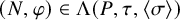 $(N, \varphi ) \in \Lambda (P,\tau , \langle \sigma \rangle )$
, we have that:
$(N, \varphi ) \in \Lambda (P,\tau , \langle \sigma \rangle )$
, we have that:
-
a)
$N\cong C_0$
; -
b)
$\gamma =\beta _i$
for an i in
$1,\cdots , k$
.


Proof. Let
 $(N, \varphi ) \in \Lambda (P,\tau , \langle \sigma \rangle )$
. We fix i, the exponent appearing in
$(N, \varphi ) \in \Lambda (P,\tau , \langle \sigma \rangle )$
. We fix i, the exponent appearing in
 $(**)$
. The composition:
$(**)$
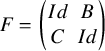
. The composition:
whose associated matrix is of type
 $F=\begin {pmatrix} A & B\\ C & D \end {pmatrix}$
, provides an isomorphism such that the polarization in
$F=\begin {pmatrix} A & B\\ C & D \end {pmatrix}$
, provides an isomorphism such that the polarization in
 $JC_0 \times JC_0$
with matrix:
$JC_0 \times JC_0$
with matrix:
 $$\begin{align*}\Lambda_0:=\begin{pmatrix} 2 \lambda_{C_0} & \lambda_{C_0} \circ \beta_i \\ \lambda_{C_0} \circ \beta_i & 2 \lambda_{C_0} \end{pmatrix}, \end{align*}$$
pulls-back to the polarization on
 $JN \times JN$
with matrix:
$JN \times JN$
with matrix:
 $$\begin{align*}\Lambda_N:=\begin{pmatrix} 2 \lambda_{N} & \lambda_{N} \circ \gamma\\ \lambda_{N} \circ \gamma & 2 \lambda_{N} \end{pmatrix}. \end{align*}$$
Considering the restriction to
 $JN\times \{0\}$
and projecting to the first factor
$JN\times \{0\}$
and projecting to the first factor
 $JC_0$
, we get a commutative diagram as follows:
$JC_0$
, we get a commutative diagram as follows:

Indeed, the dual of
 $\iota $
is
$\iota $
is
 $pr_1$
and the polarization induced by
$pr_1$
and the polarization induced by
 $\Lambda _N$
on
$\Lambda _N$
on
 $JN$
is exactly
$JN$
is exactly
 $\lambda _N$
. Therefore, the map
$\lambda _N$
. Therefore, the map
 $pr_1\circ F\circ \iota : JN\rightarrow JC_0$
satisfies that the pull-back of twice the canonical polarization on
$pr_1\circ F\circ \iota : JN\rightarrow JC_0$
satisfies that the pull-back of twice the canonical polarization on
 $JC_0$
is twice the canonical polarization on
$JC_0$
is twice the canonical polarization on
 $JN$
. Hence,
$JN$
. Hence,
 $(JN,\Theta _N)\cong (JC_0,\Theta _{C_0})$
. By the Torelli theorem,
$(JN,\Theta _N)\cong (JC_0,\Theta _{C_0})$
. By the Torelli theorem,
 $N\cong C_0$
. This proves a).
$N\cong C_0$
. This proves a).
In order to prove b), we fix an isomorphism
 $N\cong C_0$
and we look again at diagram (3.2) (by an abuse of notation we still use the letter F). The composition
$N\cong C_0$
and we look again at diagram (3.2) (by an abuse of notation we still use the letter F). The composition
 $pr_1\circ F\circ \iota : JC_0\rightarrow JC_0$
corresponds to the piece A in the matrix of F. Hence,
$pr_1\circ F\circ \iota : JC_0\rightarrow JC_0$
corresponds to the piece A in the matrix of F. Hence,
 $$\begin{align*}2\lambda_0= 2A^\vee\lambda_0 A, \end{align*}$$
that is, A preserves the polarization on
 $JC_0$
. Thus, A comes from an automorphism of
$JC_0$
. Thus, A comes from an automorphism of
 $C_0$
. By Proposition 3.8, we obtain
$C_0$
. By Proposition 3.8, we obtain
 $A=\pm Id$
. Replacing
$A=\pm Id$
. Replacing
 $\iota $
by
$\iota $
by
 $\iota _2$
(the restriction to the second factor of
$\iota _2$
(the restriction to the second factor of
 $JC_0\times JC_0$
) and, analogously,
$JC_0\times JC_0$
) and, analogously,
 $pr_1$
by
$pr_1$
by
 $pr_2$
in diagram (3.2), we obtain
$pr_2$
in diagram (3.2), we obtain
 $D=\pm Id$
. In order to study the terms B and C recall that, by assumptions (property (**)), for a certain unique i, we have
$D=\pm Id$
. In order to study the terms B and C recall that, by assumptions (property (**)), for a certain unique i, we have
 $$ \begin{align} \sigma^i\circ \varphi=\varphi\circ \begin{pmatrix} 0 & -1\\ 1 & \gamma \end{pmatrix}, \end{align} $$
and, thanks to Proposition 2.3, the same occurs for
 $\psi _i$
with
$\psi _i$
with
 $\sigma _{\beta _i}:=\begin {pmatrix} 0 & -1\\ 1 & \beta _i \end {pmatrix}$
. Therefore, we have the following diagram:
$\sigma _{\beta _i}:=\begin {pmatrix} 0 & -1\\ 1 & \beta _i \end {pmatrix}$
. Therefore, we have the following diagram:

where
 $\sigma _{\gamma }$
is the matrix in (3.3). Now, we analyze the possibilities for F.
$\sigma _{\gamma }$
is the matrix in (3.3). Now, we analyze the possibilities for F.
-
1. Let
$F=\begin {pmatrix} Id & B\\ C & Id \end {pmatrix}$
. The commutativity of the diagram above says that
$B=-C=0$
and
$\gamma =\beta _i$
. -
2. Let
$F=\begin {pmatrix} Id & B\\ C & -Id \end {pmatrix}$
in this case
$B=-C$
and
$\gamma =\beta _i$
.


And the same occurs for the other configurations. This ends the proof.
3.4. Fourth step: theta duality.
The first three steps show that the curve
 $C_0$
and the set of automorphisms
$C_0$
and the set of automorphisms
 $\{\beta _1, \ldots ,\beta _k\}$
of
$\{\beta _1, \ldots ,\beta _k\}$
of
 $JC_0$
can be recovered from the initial data
$JC_0$
can be recovered from the initial data
 $(P, \tau , \langle \sigma \rangle )$
. We shall prove that these automorphisms determine the map
$(P, \tau , \langle \sigma \rangle )$
. We shall prove that these automorphisms determine the map
 $h_0:C_0 \rightarrow \mathbb P^1$
appearing in Diagram (2.1).
$h_0:C_0 \rightarrow \mathbb P^1$
appearing in Diagram (2.1).
Let us recall the definition of the theta-dual of a subvariety X of a principally abelian variety
 $(A,\tau _A)$
, with
$(A,\tau _A)$
, with
 $\dim (X) \leq \dim A -2$
. Fix an effective theta divisor
$\dim (X) \leq \dim A -2$
. Fix an effective theta divisor
 $\Theta $
representing the polarization
$\Theta $
representing the polarization
 $\tau _{A}$
.
$\tau _{A}$
.
Definition 3.11. The theta-dual
 $T(X)$
of X is set-theoretically defined by
$T(X)$
of X is set-theoretically defined by
 $$\begin{align*}T(X)=\{a\in A \mid X\subset \Theta +a\}. \end{align*}$$
That is, we consider the set of translates of X contained in the theta divisor or, equivalently, the set of
 $a\in A$
such that X is contained in
$a\in A$
such that X is contained in
 $t_{-a}^*(\Theta )$
, where
$t_{-a}^*(\Theta )$
, where
 $t_{a}$
stands for the translation
$t_{a}$
stands for the translation
 $x\mapsto x+a$
. Notice that changing the effective divisor representing the principal polarization
$x\mapsto x+a$
. Notice that changing the effective divisor representing the principal polarization
 $T(X)$
is modified by a translation.
$T(X)$
is modified by a translation.
Pareschi and Popa gave a natural scheme structure to
 $T(X)$
for any closed reduced subscheme X (see [Reference Pareschi and Popa12, Def. 4.2]) by defining
$T(X)$
for any closed reduced subscheme X (see [Reference Pareschi and Popa12, Def. 4.2]) by defining
 $T(X)$
in terms of the Fourier–Mukai transform on A; more precisely,
$T(X)$
in terms of the Fourier–Mukai transform on A; more precisely,
 $T(X)$
becomes the support of an explicit sheaf on A. They also proved (see [Reference Pareschi and Popa12, Section 8]) that for a smooth curve N embedded in its Jacobian it holds, up to translation,
$T(X)$
becomes the support of an explicit sheaf on A. They also proved (see [Reference Pareschi and Popa12, Section 8]) that for a smooth curve N embedded in its Jacobian it holds, up to translation,
 $T(N)=-W_{g(N)-2}(N)$
, where
$T(N)=-W_{g(N)-2}(N)$
, where
 $W_{g(N)-2}(N)$
stands for the Brill–Noether locus of effective divisors of degree
$W_{g(N)-2}(N)$
stands for the Brill–Noether locus of effective divisors of degree
 $g(N)-2$
translated to
$g(N)-2$
translated to
 $JN$
by subtracting some
$JN$
by subtracting some
 $\alpha \in Pic^{g(N)-2}(N)$
. Similar results for Prym curves in their Prym varieties are obtained in [Reference Lahoz and Naranjo6].
$\alpha \in Pic^{g(N)-2}(N)$
. Similar results for Prym curves in their Prym varieties are obtained in [Reference Lahoz and Naranjo6].
The key idea in this part is to compute the theta-dual of the curve
 $\beta _i(C_0)$
embedded in
$\beta _i(C_0)$
embedded in
 $JC_0$
and use this to recover the whole map
$JC_0$
and use this to recover the whole map
 $h_0$
.
$h_0$
.
Observe that in the Jacobian
 $JC_0$
(of genus k), we can give a canonical definition of the set
$JC_0$
(of genus k), we can give a canonical definition of the set
 $T(X)$
by representing it in the torsor
$T(X)$
by representing it in the torsor
 $Pic^{k-1}(C_0)$
, where the theta divisor is canonically identified with
$Pic^{k-1}(C_0)$
, where the theta divisor is canonically identified with
 $W_{k-1}(C_0)$
. We change slightly the notation to avoid confusion, so for any subscheme
$W_{k-1}(C_0)$
. We change slightly the notation to avoid confusion, so for any subscheme
 $X\subset JC_0$
we define the following:
$X\subset JC_0$
we define the following:
Definition 3.12. The canonical theta-dual
 $T'(X)$
of
$T'(X)$
of
 $X\subset JC_0$
is set-theoretically defined by
$X\subset JC_0$
is set-theoretically defined by
 $$\begin{align*}T'(X)=\{\psi \in Pic^{k-1}(C_0) \mid X+\psi \subset \Theta^{can}= W_{k-1}(C_0)\}. \end{align*}$$
Let us fix from now on a point
 $x \in C_0$
, and consider the injection
$x \in C_0$
, and consider the injection
 $\iota _x: C_0\hookrightarrow JC_0, p\mapsto [p-x]$
. Our aim is to compute
$\iota _x: C_0\hookrightarrow JC_0, p\mapsto [p-x]$
. Our aim is to compute
 $T'(\beta _i(\iota _x(C_0)))\subset Pic^{k-1}(C_0)$
.
$T'(\beta _i(\iota _x(C_0)))\subset Pic^{k-1}(C_0)$
.
Observe that to use the definition of
 $\beta _i$
we need to see
$\beta _i$
we need to see
 $JC_0=\pi _0^*(JC_0)$
as a subvariety of P. Given a point p in
$JC_0=\pi _0^*(JC_0)$
as a subvariety of P. Given a point p in
 $C_{0}$
,
$C_{0}$
,
 $\iota _x(p)=[p-x]$
appears as
$\iota _x(p)=[p-x]$
appears as
 $[p'+j(p')-x'-j(x')]\in P$
, where
$[p'+j(p')-x'-j(x')]\in P$
, where
 $x',p'\in \widetilde C$
are preimages of
$x',p'\in \widetilde C$
are preimages of
 $x,p$
, respectively. We denote by
$x,p$
, respectively. We denote by
 $$\begin{align*}p', p^{\prime}1:=\sigma (p'),\ldots ,p^{\prime}{d-1}=p^{\prime}{2k}:=\sigma ^{d-1}(p') \end{align*}$$
the whole fiber
 $f^{-1}(f(p'))$
and analogously for
$f^{-1}(f(p'))$
and analogously for
 $x'$
. We denote by
$x'$
. We denote by
 $p_i$
(resp.
$p_i$
(resp.
 $x_i$
) the image of
$x_i$
) the image of
 $p^{\prime }i$
(resp.
$p^{\prime }i$
(resp.
 $x^{\prime }i$
) in
$x^{\prime }i$
) in
 $C_0$
. With these notations, we have:
$C_0$
. With these notations, we have:
Proposition 3.13. Assume that
 $k \ge 4$
, then the following equality holds in
$k \ge 4$
, then the following equality holds in
 $Pic^{k-1}(C_0)$
:
$Pic^{k-1}(C_0)$
:
 $$\begin{align*}T'(\beta_i(\iota_x(C_0)))=x_i+x_{d-i}+W_{k-3}(C_0). \end{align*}$$
Proof. Following the previous notation, the action of
 $\beta _i=\sigma ^i+\sigma ^{-i}$
on
$\beta _i=\sigma ^i+\sigma ^{-i}$
on
 $[p'+j(p')-x'-j(x')]$
is as follows:
$[p'+j(p')-x'-j(x')]$
is as follows:
 $$ \begin{align*} & [\sigma ^i(p')+\sigma^i(j(p'))+\sigma ^{-i}(p')+\sigma^{-i}(j(p')) -\sigma ^i(x')-\sigma^i(j(x'))-\sigma ^{-i}(x')-\sigma^{-i}(j(x'))]= \\ & [p^{\prime}i+j(p^{\prime}{d-i})+p^{\prime}{d-i}+ j(p^{\prime}{i}) - x^{\prime}i-j(x^{\prime}{d-i})-x^{\prime}{d-i}-j(x^{\prime}{i})]= \\ & (1+j)([p^{\prime}i+p^{\prime}{d-i}-x^{\prime}i-x^{\prime}{d-i}]). \end{align*} $$
Then, as element in
 $JC_0$
, we have obtained that:
$JC_0$
, we have obtained that:
 $$\begin{align*}\beta_i ( [p-x])=[p_i+p_{d-i}-x_i-x_{d-i}]. \end{align*}$$
Observe that these points describe the fiber
 $h_0^{-1}(h_0(x))$
, more precisely, as divisors:
$h_0^{-1}(h_0(x))$
, more precisely, as divisors:
 $$ \begin{align} h_0^{-1}(h_0(x))=x+x_1+\ldots +x_{d-1}. \end{align} $$
By definition,
 $\xi \in T'(\beta _i(\iota _x(C_0))) $
means that:
$\xi \in T'(\beta _i(\iota _x(C_0))) $
means that:
 $$\begin{align*}h^0(C_0,\xi + p_i+p_{d-i}-x_i-x_{d-i})>0,\qquad \text{for all } p\in C_0. \end{align*}$$
If
 $\xi $
is of the form
$\xi $
is of the form
 $x_i+x_{d-i}+E$
for some effective divisor E, the condition is satisfied trivially, hence
$x_i+x_{d-i}+E$
for some effective divisor E, the condition is satisfied trivially, hence
 $x_i+x_{d-i}+W_{k-3}(C_0)\subset T'(\beta _i(\iota _x(C_0))).$
To prove the opposite inclusion, we consider
$x_i+x_{d-i}+W_{k-3}(C_0)\subset T'(\beta _i(\iota _x(C_0))).$
To prove the opposite inclusion, we consider
 $\xi \in T'(\beta _i(\iota _x(C_0)))$
. If
$\xi \in T'(\beta _i(\iota _x(C_0)))$
. If
 $h^0(C_0, \xi -x_i-x_{d-i})>0$
, then we are done. So assume
$h^0(C_0, \xi -x_i-x_{d-i})>0$
, then we are done. So assume
 $h^0(C_0, \xi -x_i-x_{d-i})=0$
. Set
$h^0(C_0, \xi -x_i-x_{d-i})=0$
. Set
 $L:= K_{C_0}-(\xi -x_i-x_{i-d})$
. By Riemann–Roch theorem,
$L:= K_{C_0}-(\xi -x_i-x_{i-d})$
. By Riemann–Roch theorem,
 $$ \begin{align*}h^0(C_0, L)=2k-2-(k-3)-k+1=2.\end{align*} $$
Hence, L is a line bundle of degree
 $k+1$
with
$k+1$
with
 $h^0(C_0,L)=2$
and such that
$h^0(C_0,L)=2$
and such that
 $h^0(C_0, L-p_{i}-p_{d-i})>0$
for all
$h^0(C_0, L-p_{i}-p_{d-i})>0$
for all
 $p_i, p_{d-i}\in C_0$
, namely, L gives a
$p_i, p_{d-i}\in C_0$
, namely, L gives a
 $g^1_{k+1}$
whose associated map
$g^1_{k+1}$
whose associated map
 $\varphi _L$
satisfies
$\varphi _L$
satisfies
 $\varphi _L(p_i)=\varphi _L(p_{d-i})$
.
$\varphi _L(p_i)=\varphi _L(p_{d-i})$
.
Now, let us take
 $p\in C_0$
such that no points in the fiber
$p\in C_0$
such that no points in the fiber
 $h_0^{-1}(h_0(p))$
are in the base locus of L. Then this shows, as before, that
$h_0^{-1}(h_0(p))$
are in the base locus of L. Then this shows, as before, that
 $\varphi _L (p_i) = \varphi _L(p_{d-i})$
. Set now
$\varphi _L (p_i) = \varphi _L(p_{d-i})$
. Set now
 $q = p_{d-2i}$
. The same argument proves that
$q = p_{d-2i}$
. The same argument proves that
 $\varphi _L (p_{d-i}) = \varphi _L(q_i) = \varphi _L(q_{d-i}) = \varphi _L(p_{2d-3i})$
.
$\varphi _L (p_{d-i}) = \varphi _L(q_i) = \varphi _L(q_{d-i}) = \varphi _L(p_{2d-3i})$
.
Proceeding in this way, one can prove that
 $\varphi _L(p_i) = \varphi _L(p_{d-i}) =\ldots = \varphi _L(p_{i+h(d-2i)})$
for all h. Since d is an odd prime which does not divide i, we can write every element
$\varphi _L(p_i) = \varphi _L(p_{d-i}) =\ldots = \varphi _L(p_{i+h(d-2i)})$
for all h. Since d is an odd prime which does not divide i, we can write every element
 $p_j$
in the form
$p_j$
in the form
 $p_j= p_{i+h(d-2i)}$
for a certain h. This shows that the whole
$p_j= p_{i+h(d-2i)}$
for a certain h. This shows that the whole
 $h_0^{-1}(h_0(p))$
is contained in the fiber of
$h_0^{-1}(h_0(p))$
is contained in the fiber of
 $\varphi _L$
, which is impossible since
$\varphi _L$
, which is impossible since
 $h_0$
has degree
$h_0$
has degree
 $d=2k+1$
.
$d=2k+1$
.
Remark 3.14. The proposition allows recovering intrinsically the class of the divisors
 $x_i+x_{d-i}$
since there are no translations leaving invariant
$x_i+x_{d-i}$
since there are no translations leaving invariant
 $W_{k(g-1)-3}(C_0)$
. It may well happen that
$W_{k(g-1)-3}(C_0)$
. It may well happen that
 $x_i+x_{d-i}$
would belong to a
$x_i+x_{d-i}$
would belong to a
 $g^1_2$
linear series, since we have not excluded the possibility of
$g^1_2$
linear series, since we have not excluded the possibility of
 $C_0$
being hyperelliptic. Assume that this is so for a generic point in
$C_0$
being hyperelliptic. Assume that this is so for a generic point in
 $C_0$
, that is, for a generic p there is an index i such that
$C_0$
, that is, for a generic p there is an index i such that
 $h^0(C,\mathcal{O}(p_i+p_{d-i}))=2$
. We can assume that
$h^0(C,\mathcal{O}(p_i+p_{d-i}))=2$
. We can assume that
 $h^0(C,\mathcal{O}(x_1+x_{d-i}))=2$
for the fixed point x we used to embed the curve. Then
$h^0(C,\mathcal{O}(x_1+x_{d-i}))=2$
for the fixed point x we used to embed the curve. Then
 $\beta_1(p-x)=p_1+p_{d-1}-x_i-x_{d-1}$
. Replacing p for a convenient point
$\beta_1(p-x)=p_1+p_{d-1}-x_i-x_{d-1}$
. Replacing p for a convenient point
 $p'$
in the same fiber we obtain
$p'$
in the same fiber we obtain
 $\beta_1(p'-x)=p_i+p_{d-i}-x_i-x_{d-1}=0$
since both divisors represent the hyperelliptic linear series. This contradicts that
$\beta_1(p'-x)=p_i+p_{d-i}-x_i-x_{d-1}=0$
since both divisors represent the hyperelliptic linear series. This contradicts that
 $\beta_1$
is an automorphism.
$\beta_1$
is an automorphism.
Proof of Theorem 1.1.
In order to show that the Prym map
 $\mathcal {P}^d$
has generically degree one, we factorize it as
$\mathcal {P}^d$
has generically degree one, we factorize it as
 $\mathcal {P}^d_2\circ \mathcal {P}^d_1$
and we show that both maps
$\mathcal {P}^d_2\circ \mathcal {P}^d_1$
and we show that both maps
 $\mathcal {P}^d_i$
have generically degree one.
$\mathcal {P}^d_i$
have generically degree one.
Let
 $(P(\widetilde C, C), \tau )$
be a generic element in
$(P(\widetilde C, C), \tau )$
be a generic element in
 $Im(\mathcal {P}^d)$
. The first three steps of the proof are devoted to the generic injectivity of
$Im(\mathcal {P}^d)$
. The first three steps of the proof are devoted to the generic injectivity of
 $\mathcal {P}^d_2$
. First, we show that the triplet
$\mathcal {P}^d_2$
. First, we show that the triplet
 $(P(\widetilde C, C), \tau , \sigma )$
is uniquely determined by
$(P(\widetilde C, C), \tau , \sigma )$
is uniquely determined by
 $(P(\widetilde C, C), \tau )$
. In the second step, we show that the only possible automorphisms of
$(P(\widetilde C, C), \tau )$
. In the second step, we show that the only possible automorphisms of
 $JC_0$
are
$JC_0$
are
 $\pm Id$
. This allows us to prove in the third step, that the fiber of
$\pm Id$
. This allows us to prove in the third step, that the fiber of
 $\mathcal {P}^d_2$
above
$\mathcal {P}^d_2$
above
 $(P(\widetilde C, C), \tau )$
is given by the element
$(P(\widetilde C, C), \tau )$
is given by the element
 $(C_0, \beta _1, \dots , \beta _k)$
.
$(C_0, \beta _1, \dots , \beta _k)$
.
The last step is devoted to the generic injectivity of
 $\mathcal {P}^d_1$
. Let
$\mathcal {P}^d_1$
. Let
 $(C_0, \beta _1, \dots , \beta _k)$
be a generic element in
$(C_0, \beta _1, \dots , \beta _k)$
be a generic element in
 $Im(\mathcal {P}^d_1)$
. According to Proposition 3.13; for a fixed
$Im(\mathcal {P}^d_1)$
. According to Proposition 3.13; for a fixed
 $x\in C_0$
, we obtain intrinsically the subset
$x\in C_0$
, we obtain intrinsically the subset
 $x_i+x_{d-i}+W_{k-3}(C_0)$
. A classical result of Weil (cf. [Reference Weil14, Hilfssatz 3]) states that
$x_i+x_{d-i}+W_{k-3}(C_0)$
. A classical result of Weil (cf. [Reference Weil14, Hilfssatz 3]) states that
 $W_{k-3}(C_0)$
is not ‘translation invariant’, that is, if
$W_{k-3}(C_0)$
is not ‘translation invariant’, that is, if
 $\alpha \in JC_0$
satisfies that
$\alpha \in JC_0$
satisfies that
 $\alpha + W_{k-3}(C_0)=W_{k-3}(C_0)$
, then
$\alpha + W_{k-3}(C_0)=W_{k-3}(C_0)$
, then
 $\alpha =0$
. This says that
$\alpha =0$
. This says that
 $x_i+x_{d-i}$
is uniquely determined in
$x_i+x_{d-i}$
is uniquely determined in
 $C_0$
. Varying
$C_0$
. Varying
 $i=1,\ldots ,k$
and using (3.5), we get that for all
$i=1,\ldots ,k$
and using (3.5), we get that for all
 $x\in C_0$
the fiber of
$x\in C_0$
the fiber of
 $h_0$
containing x is recovered. Now, by construction the map
$h_0$
containing x is recovered. Now, by construction the map
 $h_0$
is ramified over six points in
$h_0$
is ramified over six points in
 ${\mathbb P}^1$
, which are also the images of the Weierstrass points of C by
${\mathbb P}^1$
, which are also the images of the Weierstrass points of C by
 $\varepsilon $
. Therefore,
$\varepsilon $
. Therefore,
 $\varepsilon : C\rightarrow \mathbb P^1$
is determined by
$\varepsilon : C\rightarrow \mathbb P^1$
is determined by
 $h_0$
. The fiber product of
$h_0$
. The fiber product of
 $\varepsilon : C\rightarrow \mathbb P^1$
and
$\varepsilon : C\rightarrow \mathbb P^1$
and
 $h_0:C_0 \rightarrow \mathbb P^1$
gives the map
$h_0:C_0 \rightarrow \mathbb P^1$
gives the map
 $\widetilde C \rightarrow C$
. This finishes the proof.
$\widetilde C \rightarrow C$
. This finishes the proof.
4. Case
$d=9$

This section is devoted to the analysis of the case
 $d=9$
, which is no longer a prime number. Due to the structure of the dihedral group
$d=9$
, which is no longer a prime number. Due to the structure of the dihedral group
 $D_9$
, the corresponding diagram is more complicated since new intermediate quotients of the curve
$D_9$
, the corresponding diagram is more complicated since new intermediate quotients of the curve
 $\widetilde C$
and of the curves
$\widetilde C$
and of the curves
 $C_i$
appear. Indeed, the situation can be summarized in the following diagram:
$C_i$
appear. Indeed, the situation can be summarized in the following diagram:

The curves
 $C_i$
correspond to the quotients
$C_i$
correspond to the quotients
 $\widetilde C/ \langle j \sigma ^i\rangle $
, the curve
$\widetilde C/ \langle j \sigma ^i\rangle $
, the curve
 $C':=\widetilde C/\langle \sigma ^3\rangle $
and, finally, the curves
$C':=\widetilde C/\langle \sigma ^3\rangle $
and, finally, the curves
 $E_i$
are obtained as
$E_i$
are obtained as
 $\widetilde C/\langle j\sigma ^i, \sigma ^3\rangle $
. Hence,
$\widetilde C/\langle j\sigma ^i, \sigma ^3\rangle $
. Hence,
 $E_i$
and
$E_i$
and
 $ E_j$
are exactly the same curve if
$ E_j$
are exactly the same curve if
 $i-j$
is a multiple of
$i-j$
is a multiple of
 $3$
. The map
$3$
. The map
 $f'$
is étale of degree 3, while the maps
$f'$
is étale of degree 3, while the maps
 $\widetilde C \rightarrow E_i$
(composing
$\widetilde C \rightarrow E_i$
(composing
 $\widetilde C \rightarrow C_i$
with
$\widetilde C \rightarrow C_i$
with
 $C_i\rightarrow E_i$
) are Galois of degree 6 with Galois group
$C_i\rightarrow E_i$
) are Galois of degree 6 with Galois group
 $\langle j\sigma ^i, \sigma ^3\rangle \cong D_3$
. We have that
$\langle j\sigma ^i, \sigma ^3\rangle \cong D_3$
. We have that
 $g(C')=4$
,
$g(C')=4$
,
 $g(C_i)=4$
and
$g(C_i)=4$
and
 $g(E_i)=1$
. By congruence modulo 3, it is sufficient to consider the first three quotient curves
$g(E_i)=1$
. By congruence modulo 3, it is sufficient to consider the first three quotient curves
 $C_0, C_1,C_2$
(respectively,
$C_0, C_1,C_2$
(respectively,
 $E_0, E_1, E_2$
). Moreover, since the three dihedral groups
$E_0, E_1, E_2$
). Moreover, since the three dihedral groups
 $\langle j, \sigma ^3\rangle , \langle j\sigma , \sigma ^3\rangle $
, and
$\langle j, \sigma ^3\rangle , \langle j\sigma , \sigma ^3\rangle $
, and
 $\langle j\sigma ^2, \sigma ^3\rangle $
are conjugated in
$\langle j\sigma ^2, \sigma ^3\rangle $
are conjugated in
 $D_9$
, all the curves
$D_9$
, all the curves
 $E_i$
are isomorphic. Finally, notice that the non-Galois degree 9 maps
$E_i$
are isomorphic. Finally, notice that the non-Galois degree 9 maps
 $h_i: C_i\rightarrow {\mathbb P}^1$
factor as noncyclic triple covers
$h_i: C_i\rightarrow {\mathbb P}^1$
factor as noncyclic triple covers
 $f_i:C_i\rightarrow E_i$
composed with some degree 3 maps
$f_i:C_i\rightarrow E_i$
composed with some degree 3 maps
 $E_i\rightarrow {\mathbb P}^1$
ramified exactly over the Weiestrass points of C. The map
$E_i\rightarrow {\mathbb P}^1$
ramified exactly over the Weiestrass points of C. The map
 $f_0: C_0\rightarrow E_0$
decomposes
$f_0: C_0\rightarrow E_0$
decomposes
 $JC_0$
up to isogeny as the product
$JC_0$
up to isogeny as the product
 $ E_0\times P(C_0,E_0)$
, where
$ E_0\times P(C_0,E_0)$
, where
 $P(C_0,E_0)$
is the three-dimensional abelian variety defined as the Prym variety associated with
$P(C_0,E_0)$
is the three-dimensional abelian variety defined as the Prym variety associated with
 $f_0$
.
$f_0$
.
A step-by-step analysis of Proposition 2.2 and Proposition 2.3 shows that they remain true in case
 $d=9$
too. Indeed, we have:
$d=9$
too. Indeed, we have:
Proposition 4.1. For
 $i=1,\dots , 4$
the following properties hold.
$i=1,\dots , 4$
the following properties hold.
-
1. The automorphisms
$\beta _i=\sigma ^i+\sigma ^{-i}$
restrict to automorphisms of
$JC_0$
. -
2. The maps
$\psi _i: JC_0\times JC_0\rightarrow P$
, sending
$(x,y)$
to
$x+\sigma ^i(y)$
are isomorphisms of polarized abelian varieties such that-
•
$\psi _i ^{\vee }\circ \lambda _{\tau } \circ \psi _i = \begin {pmatrix} 2 \lambda _{C_0} & \lambda _{C_0} \circ \beta _i \\ \lambda _{C_0} \circ \beta _i & 2 \lambda _{C_0} \end {pmatrix}$
; -
•
$\psi _i ^{-1}\circ \sigma ^i \circ \psi _i = \begin {pmatrix} 0 &-1\\ 1 &\beta _i \end {pmatrix}$
.
-


Since both
 $\pi _0$
and
$\pi _0$
and
 $f_0$
are ramified maps, we have the inclusions
$f_0$
are ramified maps, we have the inclusions
 $E_0\subset JC_0\subset J\widetilde C$
. More precisely, we have the following:
$E_0\subset JC_0\subset J\widetilde C$
. More precisely, we have the following:
Proposition 4.2. The map
 $f_0: C_0\rightarrow E_0$
is given by the composition
$f_0: C_0\rightarrow E_0$
is given by the composition
 $C_0\hookrightarrow JC_0\xrightarrow {(1+\beta _3)} E_0$
. In particular,
$C_0\hookrightarrow JC_0\xrightarrow {(1+\beta _3)} E_0$
. In particular,
 $E_0=Im(1+j)(1+\beta _3).$
Proof. Let us focus on the following part of diagram (4.1):

Let
 $$\begin{align*}x, \sigma(x), \dots, \sigma^8(x)\quad \text{resp.} \quad jx, \sigma(jx), \dots, \sigma^8(jx) \end{align*}$$
be the whole fibers
 $f^{-1}(f(x))$
, resp.
$f^{-1}(f(x))$
, resp.
 $f^{-1}(f(jx))$
. By construction, the map
$f^{-1}(f(jx))$
. By construction, the map
 $f'$
identifies
$f'$
identifies
 $[x]=[\sigma ^3(x)]= [\sigma ^6(x)]$
. By the commutativity of the diagram, we also have
$[x]=[\sigma ^3(x)]= [\sigma ^6(x)]$
. By the commutativity of the diagram, we also have
 $E_0= C'/\langle j\rangle $
. Thus, in
$E_0= C'/\langle j\rangle $
. Thus, in
 $E_0$
, we get the
$E_0$
, we get the
 $6:1$
identification
$6:1$
identification
 $$ \begin{align} [x]=[\sigma^3(x)]= [\sigma^6(x)]=[jx]=[j\sigma^3(x)]= [j\sigma^6(x)]. \end{align} $$
Obviously, the analogous holds true for the fiber of
 $\sigma (x) $
and of
$\sigma (x) $
and of
 $\sigma ^2(x)$
.
$\sigma ^2(x)$
.
By definition, in
 $C_0$
, we have
$C_0$
, we have
 $[x]=[jx]$
,
$[x]=[jx]$
,
 $[\sigma ^3(x)]=[j\sigma ^3(x)]=[\sigma ^6(jx)]$
, and
$[\sigma ^3(x)]=[j\sigma ^3(x)]=[\sigma ^6(jx)]$
, and
 $[\sigma ^6(x)]=[j\sigma ^6(x)]=[\sigma ^3(jx)]$
. The commutativity of Equation (4.2), together with Equation (4.3), gives us the 3:1 map
$[\sigma ^6(x)]=[j\sigma ^6(x)]=[\sigma ^3(jx)]$
. The commutativity of Equation (4.2), together with Equation (4.3), gives us the 3:1 map
 $f_0$
. As we already know,
$f_0$
. As we already know,
 $JC_0=Im(1+j)$
. Thus, we get
$JC_0=Im(1+j)$
. Thus, we get
 $JE_0\cong E_0=Im(1+j)(1+\sigma ^3+\sigma ^6)$
. Finally, it is easy to check that composing with the natural injection
$JE_0\cong E_0=Im(1+j)(1+\sigma ^3+\sigma ^6)$
. Finally, it is easy to check that composing with the natural injection
 $\iota _x: C_0\hookrightarrow JC_0, \, p\mapsto [p-x]$
, we obtain the map
$\iota _x: C_0\hookrightarrow JC_0, \, p\mapsto [p-x]$
, we obtain the map
 $f_0$
.
$f_0$
.
As a consequence, we get the following:
Proposition 4.3. The automorphisms
 $\beta _1,\beta _2,\beta _4$
restrict to
$\beta _1,\beta _2,\beta _4$
restrict to
 $-Id$
on
$-Id$
on
 $E_0$
, while
$E_0$
, while
 $\beta _3$
acts as multiplication by 2.
$\beta _3$
acts as multiplication by 2.
Proof. It is a straightforward computation using that
 $E_0=Im (1+j)(1+\sigma ^3+\sigma ^6)$
, the fact that
$E_0=Im (1+j)(1+\sigma ^3+\sigma ^6)$
, the fact that
 $\beta _i$
commutes with
$\beta _i$
commutes with
 $(1+j)$
and that
$(1+j)$
and that
 $1+\sigma +\dots +\sigma ^8=0$
on
$1+\sigma +\dots +\sigma ^8=0$
on
 $J\widetilde C$
.
$J\widetilde C$
.
Let
 $\xi $
be a ninth primitive root of unity. In what follows, we want to describe more explicitly the automorphisms
$\xi $
be a ninth primitive root of unity. In what follows, we want to describe more explicitly the automorphisms
 $\beta _i$
. First, we recall that the following equalities hold:
$\beta _i$
. First, we recall that the following equalities hold:
 $$ \begin{align} [\mathbb{Q}(\xi): \mathbb{Q}]= [\mathbb{Q}(\xi): \mathbb{Q}(\xi+\xi^{-1})][\mathbb{Q}(\xi+\xi^{-1}): \mathbb{Q}]=2\cdot 3=6. \end{align} $$
The action of
 $\sigma $
on
$\sigma $
on
 $H^0(\widetilde C, \omega _{\widetilde C})$
decomposes as follows ([Reference Lange and Ortega7, Section 3])
$H^0(\widetilde C, \omega _{\widetilde C})$
decomposes as follows ([Reference Lange and Ortega7, Section 3])
 $$ \begin{align} H^0(\widetilde C, \omega_{\widetilde C})= \bigoplus_{i=0}^8 H^0( C, \omega_{ C}\otimes \eta^i), \end{align} $$
where
 $H^0( C, \omega _{ C}\otimes \eta ^i)$
is the eigenspace corresponding to the eigenvalue
$H^0( C, \omega _{ C}\otimes \eta ^i)$
is the eigenspace corresponding to the eigenvalue
 $\xi ^i$
. This yields the following:
$\xi ^i$
. This yields the following:
Proposition 4.4. The automorphisms
 $\beta _i$
act on
$\beta _i$
act on
 $T_0JC_0$
as the diagonal matrices
$T_0JC_0$
as the diagonal matrices
 $$ \begin{align*}diag(\xi^i+\xi^{-i}, \xi^{2i}+\xi^{-2i}, \xi^{3i}+\xi^{-3i}, \xi^{4i}+\xi^{-4i}).\end{align*} $$
Therefore, up to permutation of the eigenspaces, the automorphisms
 $\beta _1,\beta _2,\beta _4$
correspond to the matrix
$\beta _1,\beta _2,\beta _4$
correspond to the matrix
 ${diag}(\xi +\xi ^{8}, \xi ^2+\xi ^{7}, \xi ^4+\xi ^5, -1)$
while
${diag}(\xi +\xi ^{8}, \xi ^2+\xi ^{7}, \xi ^4+\xi ^5, -1)$
while
 $\beta _3$
is given by
$\beta _3$
is given by
 $diag(-1,-1,-1,2)$
. As an immediate consequence, we get the following:
$diag(-1,-1,-1,2)$
. As an immediate consequence, we get the following:
Proposition 4.5. The Prym variety
 $P(C_0, E_0)$
is of
$P(C_0, E_0)$
is of
 $GL_2$
-type.
$GL_2$
-type.
Proof. Using the description of the automorphisms
 $\beta _i: JC_0\rightarrow JC_0$
as a diagonal matrix, together with Proposition 4.3, we obtain that they restrict to automorphisms of
$\beta _i: JC_0\rightarrow JC_0$
as a diagonal matrix, together with Proposition 4.3, we obtain that they restrict to automorphisms of
 $P(C_0, E_0)$
. Therefore,
$P(C_0, E_0)$
. Therefore,
 $F:=\mathbb {Q}(\xi +\xi ^{-1})$
is embedded in
$F:=\mathbb {Q}(\xi +\xi ^{-1})$
is embedded in
 $End_0(P(C_0, E_0))$
. Since, by Equation (4.4), F is a totally real cubic field, we conclude that
$End_0(P(C_0, E_0))$
. Since, by Equation (4.4), F is a totally real cubic field, we conclude that
 $P(C_0, E_0)$
is of
$P(C_0, E_0)$
is of
 $GL_2$
-type.
$GL_2$
-type.
Now, we have all the ingredients to prove the following:
Theorem 4.6. The Prym map
 $\mathcal {P}_9: \mathcal {R}^9\rightarrow \mathcal {A}_8^{(1,\dots ,1,9)}$
is generically injective.
$\mathcal {P}_9: \mathcal {R}^9\rightarrow \mathcal {A}_8^{(1,\dots ,1,9)}$
is generically injective.
Proof. The proof traces the one given in case of
 $d, k$
prime numbers. The main difference here is that instead of recovering
$d, k$
prime numbers. The main difference here is that instead of recovering
 $h_0: C_0\rightarrow {\mathbb P}^1$
, we recover the map
$h_0: C_0\rightarrow {\mathbb P}^1$
, we recover the map
 $f_0: C_0\rightarrow E_0$
.
$f_0: C_0\rightarrow E_0$
.
Let
 $(P,\tau )$
be a general element in
$(P,\tau )$
be a general element in
 $Im(\mathcal {P}_9)$
. By Proposition 3.1, we obtain the triplet
$Im(\mathcal {P}_9)$
. By Proposition 3.1, we obtain the triplet
 $(P, \tau , \langle \sigma \rangle )$
. Thus, as in Equation (3.1), we define the set
$(P, \tau , \langle \sigma \rangle )$
. Thus, as in Equation (3.1), we define the set
 $\Lambda (P,\tau , \langle \sigma \rangle )$
. Since, by Proposition 4.1 also in case of
$\Lambda (P,\tau , \langle \sigma \rangle )$
. Since, by Proposition 4.1 also in case of
 $d=9$
the maps
$d=9$
the maps
 $\psi _i$
are isomorphisms of polarized abelian varieties, we can use Proposition 3.10 to recover the curve
$\psi _i$
are isomorphisms of polarized abelian varieties, we can use Proposition 3.10 to recover the curve
 $C_0$
. Using the same proposition (the second part of its proof where property
$C_0$
. Using the same proposition (the second part of its proof where property
 $(\ast \ast $
) is exploited) one can show that
$(\ast \ast $
) is exploited) one can show that
 $\gamma $
is of the form
$\gamma $
is of the form
 $\phi ^{-1}\beta _i\phi $
for an
$\phi ^{-1}\beta _i\phi $
for an
 $i \in \{ 1,2,3,4 \}$
and for
$i \in \{ 1,2,3,4 \}$
and for
 $\phi $
an automorphism of
$\phi $
an automorphism of
 $JC_0$
(compatible with the principal polarization, but this will not be used).
$JC_0$
(compatible with the principal polarization, but this will not be used).
Now, using the obtained automorphisms
 $\gamma $
’s, we consider the one-dimensional images
$\gamma $
’s, we consider the one-dimensional images
 $Im(\gamma +Id)$
. By Proposition 4.3, these images are the curves
$Im(\gamma +Id)$
. By Proposition 4.3, these images are the curves
 $E_0$
or
$E_0$
or
 $\phi (E_0)$
. We do not take into account higher-dimensional images, that is, the ones coming from
$\phi (E_0)$
. We do not take into account higher-dimensional images, that is, the ones coming from
 $\beta _i$
or from
$\beta _i$
or from
 $\phi ^{-1}\beta _i\phi $
for
$\phi ^{-1}\beta _i\phi $
for
 $i=1,2,4$
. By Proposition 4.2, we get the map
$i=1,2,4$
. By Proposition 4.2, we get the map
 $f_0$
in case of
$f_0$
in case of
 $\gamma =\beta _3$
, resp. the map
$\gamma =\beta _3$
, resp. the map
 $C_0\rightarrow \phi (E_0)$
in case of
$C_0\rightarrow \phi (E_0)$
in case of
 $\gamma =\phi ^{-1}\beta _3\phi $
. In this way, we conclude the result. Indeed, by definition, the Galois closure of
$\gamma =\phi ^{-1}\beta _3\phi $
. In this way, we conclude the result. Indeed, by definition, the Galois closure of
 $\widetilde C\rightarrow E_0$
does not depend on the automorphism of the base. This yields the element
$\widetilde C\rightarrow E_0$
does not depend on the automorphism of the base. This yields the element
 $\widetilde C\rightarrow C \in \mathcal {R}^9$
we are looking for.
$\widetilde C\rightarrow C \in \mathcal {R}^9$
we are looking for.
5. Case
$d=13$

This section is devoted to the analysis of the case
 $d=13$
, where d is a prime number, whereas
$d=13$
, where d is a prime number, whereas
 $k=6$
no longer is. This prevents us to use the full Proposition 3.10, so one has to characterize the set
$k=6$
no longer is. This prevents us to use the full Proposition 3.10, so one has to characterize the set
 $\Lambda (P,\tau , \langle \sigma \rangle )$
defined as in Equation (3.1). The diagram to keep in mind is the following:
$\Lambda (P,\tau , \langle \sigma \rangle )$
defined as in Equation (3.1). The diagram to keep in mind is the following:

We recall that
 $g(C_0)=6$
and that
$g(C_0)=6$
and that
 $\beta _i=\sigma ^i+\sigma ^{-i}$
are automorphisms of
$\beta _i=\sigma ^i+\sigma ^{-i}$
are automorphisms of
 $JC_0$
not preserving the polarization. The second step of Section 3 yields the following:
$JC_0$
not preserving the polarization. The second step of Section 3 yields the following:
Proposition 5.1. The Jacobian variety
 $JC_0$
is of
$JC_0$
is of
 $GL_2$
-type which is either simple or is isogenous to
$GL_2$
-type which is either simple or is isogenous to
 $X^r$
, where X is a simple abelian variety of
$X^r$
, where X is a simple abelian variety of
 $GL_2$
-type and
$GL_2$
-type and
 $r\in \mathbb {N}$
. Moreover, any automorphism of the curve
$r\in \mathbb {N}$
. Moreover, any automorphism of the curve
 $C_0$
is an involution.
$C_0$
is an involution.
We have the following:
Corollary 5.2. For a general
 $\widetilde C\rightarrow C$
, the Jacobian variety
$\widetilde C\rightarrow C$
, the Jacobian variety
 $JC_0$
is either simple or isogenous to the square of a simple abelian threefold. In the first case, any involution induced on
$JC_0$
is either simple or isogenous to the square of a simple abelian threefold. In the first case, any involution induced on
 $JC_0$
from an automorphism of
$JC_0$
from an automorphism of
 $C_0$
is
$C_0$
is
 $\pm Id$
.
$\pm Id$
.
Proof. Indeed, we have to exclude that
 $JC_0$
is one of the following cases:
$JC_0$
is one of the following cases:
-
1.
$E^6$
, where E is an elliptic curve, -
2.
$S^3$
, where S is a
$GL_2$
-type abelian surface.


This follows from a dimensional argument. The first case is excluded because the moduli of elliptic curves is one-dimensional. In the second case the moduli of abelian surfaces is three-dimensional, but the endomorphism algebra of the generic element is
 $\mathbb {Z}$
, and this is not compatible with our assumptions on the endomorphism algebra of S, so it can be also ruled out.
$\mathbb {Z}$
, and this is not compatible with our assumptions on the endomorphism algebra of S, so it can be also ruled out.
Thus, in order to conclude the generic injectivity of
 $\mathcal P_{13}$
, it only remains to exclude the case
$\mathcal P_{13}$
, it only remains to exclude the case
 $JC_0\sim T^2$
(which prevents us to obtain a result as in Proposition 3.10). Such configuration is realized when an involution
$JC_0\sim T^2$
(which prevents us to obtain a result as in Proposition 3.10). Such configuration is realized when an involution
 $\phi $
acts on
$\phi $
acts on
 $C_0$
with quotient a genus 3 curve
$C_0$
with quotient a genus 3 curve
 $C^{\prime }0$
. That is, the 2:1 covering
$C^{\prime }0$
. That is, the 2:1 covering
 $C_0\rightarrow C^{\prime }0=C_0/\langle \phi \rangle $
is branched in two points and such that
$C_0\rightarrow C^{\prime }0=C_0/\langle \phi \rangle $
is branched in two points and such that
 $T\sim JC^{\prime }0\sim P(C_0,C^{\prime }0)$
is a
$T\sim JC^{\prime }0\sim P(C_0,C^{\prime }0)$
is a
 $GL_2$
-type threefold. One should then show that this does not occur for the general curve
$GL_2$
-type threefold. One should then show that this does not occur for the general curve
 $C_0$
of the three-dimensional family appearing as a quotient of
$C_0$
of the three-dimensional family appearing as a quotient of
 $\tilde C$
.
$\tilde C$
.
Acknowledgements
We thank X. Guitart for valuable information about abelian varieties of
 $GL_2$
-type and B. van Geemen, G. Farkas, G.P. Pirola and P. Borówka for stimulating discussions on the subject. Moreover, we thank the anonymous referee for a very careful reading of the paper and suggestions in the presentation.
$GL_2$
-type and B. van Geemen, G. Farkas, G.P. Pirola and P. Borówka for stimulating discussions on the subject. Moreover, we thank the anonymous referee for a very careful reading of the paper and suggestions in the presentation.
Competing interests
The authors have no competing interest to declare.
Financial support
This material is based upon work supported by the Swedish Research Council under grant no. 2021-06594 while the second author was in residence at Institut Mittag-Leffler in Djursholm, Sweden, during the semester September–December of 2021. The first and the third authors were partially supported by the Proyecto de Investigación PID2019-104047GB-100. The third author is a member of GNSAGA (INdAM) and was partially supported by INdAM-GNSAGA project CUP E55F22000270001.


 Open access