


1. Introduction
Material Extrusion (MEX) has become one of the most widely used polymer Additive Manufacturing (AM) processes due to its low cost, material versatility and accessibility (Reference Dua, Rashad, Spears, Dunn and MaxwellDua et al., 2021; Reference Enriconi, Rodriguez, Araújo, Rocha, García-Martín, Ribeiro, Pisonero and Rodríguez-MartínEnriconi et al., 2025; Reference Oleff, Küster, Stonis and OvermeyerOleff et al., 2021). Recent comprehensive reviews underline both the potential of MEX for functional applications and the importance of understanding its process–structure–property relationships (Reference Abdelhamid, Mohamed and KelouwaniAbdelhamid et al., 2024; Reference Dua, Rashad, Spears, Dunn and MaxwellDua et al., 2021; Reference Enriconi, Rodriguez, Araújo, Rocha, García-Martín, Ribeiro, Pisonero and Rodríguez-MartínEnriconi et al., 2025; Reference Oleff, Küster, Stonis and OvermeyerOleff et al., 2021; Reference ZanjanijamZanjanijam, 2020).
Material-extrusion polymers range from standard thermoplastics to high-performance materials such as polyetheretherketone (PEEK), polyetherimide (PEI) and polyamide (PA), which offer high strength and elevated service temperatures (Reference Dua, Rashad, Spears, Dunn and MaxwellDua et al., 2021; Reference SinghSingh, 2024; Reference Wang, Müller, Rumjahn, Schmidt and SchwitallaWang et al., 2021; Reference ZanjanijamZanjanijam, 2020). Their mechanical behaviour depends strongly on processing conditions and the thermal history experienced during printing (Reference Enriconi, Rodriguez, Araújo, Rocha, García-Martín, Ribeiro, Pisonero and Rodríguez-MartínEnriconi et al., 2025; Reference Keim, Young, Hanson, Collins and McClainKeim et al., 2025; Reference Lambiase, Pace, Andreucci and PaolettiLambiase et al., 2024; Reference Wang, Müller, Rumjahn, Schmidt and SchwitallaWang et al., 2021; Reference ZanjanijamZanjanijam, 2020). Fatigue studies show that printed polymers exhibit anisotropy, but fatigue life can be significantly improved through optimized parameters (Reference Rendas, Imperadeiro, Martins and SoaresRendas et al., 2024; Reference Safai, Cuellar, Smit and ZadpoorSafai et al., 2019; Reference Shanmugam, Das, Babu, Marimuthu, Veerasimman, Johnson, Neisiany, Hedenqvist, Ramakrishna and BertoShanmugam et al., 2021).
High-performance polymers, especially PEEK, demonstrate high fatigue strength and are suitable for functional end-use components (Reference Dua, Rashad, Spears, Dunn and MaxwellDua et al., 2021; Reference Nyman, Lehto, Kukko, Kestilä and KallioNyman et al., 2024; Reference Rendas, Imperadeiro, Martins and SoaresRendas et al., 2024; Reference Wang, Müller, Rumjahn, Schmidt and SchwitallaWang et al., 2021).
In high-temperature printing, interlayer adhesion is governed by thermal contact at deposition; insufficient reheating weakens the bond, whereas higher interface temperatures promote polymer diffusion and stronger welds (Reference Keim, Young, Hanson, Collins and McClainKeim et al., 2025; Reference Lambiase, Pace, Andreucci and PaolettiLambiase et al., 2024; Reference Morales, Fleck and RhoadsMorales et al., 2018; Reference OmerOmer, 2025; Reference VanaeiVanaei, 2021). Controlled cooling and adequate extrusion temperatures improve layer fusion, while excessive heat risks degradation (Reference Keim, Young, Hanson, Collins and McClainKeim et al., 2025; Reference Lambiase, Pace, Andreucci and PaolettiLambiase et al., 2024; Reference Morales, Fleck and RhoadsMorales et al., 2018;). Recent work further highlights strong thermal–mechanical coupling in high-temperature extrusion and the influence of local cooling and convection on final properties (Reference Keim, Young, Hanson, Collins and McClainKeim et al., 2025; Reference McBean, Yi, Chaplin and GhitaMcBean et al., 2025; Reference VanaeiVanaei, 2021).
Process monitoring—including optical, acoustic, thermal and force-based sensing—is increasingly adopted to improve repeatability and traceability in MEX (Reference Ferraris, Zhang and Van HoorewederFerraris et al., 2019; Reference Fu, Downey, Yuan, Pratt and BalogunFu et al., 2021; Reference Oleff, Küster, Stonis and OvermeyerOleff et al., 2021). Machine Learning (ML) enhances defect detection, parameter optimization, and process–structure–property prediction (Reference Abdelhamid, Mohamed and KelouwaniAbdelhamid et al., 2024; Reference Nikooharf, Shirinbayan, Arabkoohi, Bahlouli, Fitoussi and BenfrihaNikooharf et al., 2024). Recent reviews on polymer AM emphasise the role of data-driven and physics-informed models for linking thermal histories, process conditions and mechanical performance across extrusion-based processes (Reference Abdelhamid, Mohamed and KelouwaniAbdelhamid et al., 2024; Reference Enriconi, Rodriguez, Araújo, Rocha, García-Martín, Ribeiro, Pisonero and Rodríguez-MartínEnriconi et al., 2025; Reference Nikooharf, Shirinbayan, Arabkoohi, Bahlouli, Fitoussi and BenfrihaNikooharf et al., 2024). Recent research shows the temperature effect on Ultimate Tensile Strength (UTS), strain and Young’s Modulus when printing Polyamide 6-CF on a low-cost actively heated printer (Reference ØrnesØrnes et al., 2026). Investigating processing temperatures from 67 to 165°C, material properties differed within the ranges 7.55 to 36.04 MPa, 1650 to 3893 MPa and 0.00450 to 0.0095 for UTS, Young’s Modulus and strain respectively. Reference Seppala and MiglerSeppala and Migler (2016) identified that materials mechanical properties are contingent upon the layer bonding. Of the two layers in a bonding process the lower layer will always have the lowest temperature. Therefore, this study aims to measure the temperature of that layer right before deposition, denoted Pre Deposition layer Temperature (PDT) as it will be the decisive factor for layer bonding.
The impact of temperature in component manufacturing is therefore crucial, and implementation of temperature monitoring systems will aid, process control and certification (Reference Fu, Downey, Yuan, Pratt and BalogunFu et al., 2021; Reference McBean, Yi, Chaplin and GhitaMcBean et al., 2025; Reference VanaeiVanaei, 2021). Infrared thermography has proven effective for tracking cooling behaviour, interface temperature, and their influence on mechanical properties (Reference Conceição, Fonseca and ThiréConceição et al., 2025; Reference Ferraris, Zhang and Van HoorewederFerraris et al., 2019; Reference Seppala and MiglerSeppala & Migler, 2016), and is already used industrially for real-time temperature monitoring (Reference Fu, Downey, Yuan, Pratt and BalogunFu et al., 2021; Reference McBean, Yi, Chaplin and GhitaMcBean et al., 2025). High-temperature printers, however, often require adaptations such as external camera mounting or additional openings to protect sensors from overheating.
This paper presents a temperature monitoring system for MEX. The presented system was developed on a highly accessible low-cost printer to enable faster prototyping and data gathering. The system captures the PDT and documents it by exporting a CSV file containing the thermal manufacturing data.
These data can be used by engineers and designers to understand the load-bearing capabilities of their products, enabling them to optimize for weight, implement additional functions, and apply the product in load-bearing applications. To the best of the authors’ knowledge, this specific method of live nozzle tracking for PDT extraction using low-cost hardware has not been extensively documented.The documentation also allows for user testing with prototypes rapidly manufactured by MEX without undue risk of injury due to component critical failures (Reference Eikevåg, Auernhammer, Elverum, Dybvik and SteinertEikevåg et al., 2024).
2. Method
Our method aims to explore how to track PDT in MEX. Additionally, the aim is to explore the accuracy of the tracking, aiming for system implementation in high temperature printing.
2.1. Exploring tracking of the nozzle
To extract PDT values live during printing it is essential to track the location of the print head. To achieve this, two tracking methods were explored: 1) ML by Convolutional Neural Network (CNN) and 2) ML by OpenCV, which will be referred to as the Hottest point method.
2.1.1. Method 1: machine learning approach
We used a supervised learning approach based on a CNN. The model takes thermal images as input and predicts the corresponding
 $$\left( {x,y} \right)$$
coordinates. Since the target values are continuous, the problem is formulated as a regression task. The network is trained using the Mean Squared Error (MSE) loss function and the Adam optimizer.
$$\left( {x,y} \right)$$
coordinates. Since the target values are continuous, the problem is formulated as a regression task. The network is trained using the Mean Squared Error (MSE) loss function and the Adam optimizer.
To build the dataset, we captured approximately 1200 images per model during the printing process, under varying angles, lighting and temperature conditions. Each image was manually annotated with the nozzle’s position. Once the dataset was prepared, we trained a model to recognize the nozzle based on its shape and temperature profile. Figure 1 shows images used for the training (Figure 1(a) and (b)) and an example of model testing (Figure 1(c)), where the ML algorithm failed to capture the nozzle location. For this model, the predicted red point was often misplaced. The model was trained with an Inferno colour map and a temperature range of 80-150 °C. This temperature range made possible to suppress the background to improve feature extraction. For evaluation, the model was tested on static images from the data set, video sequences from the data set, and finally live camera input. While performance on static images was acceptable, results on video sequences were poor. The main limitation of this method was the camera itself: it only detects temperature values, rather than true colours or detailed shapes. As a result, any variation in temperature changed the apparent colour of the nozzle, leading to inconsistent detection.
ML model with Inferno colour map. (a) picture for training, with the fans on, (b) picture for training, with the fans off, (c) result of the model 1 (d) result of model 2

With the same setup and settings, the nozzle appears purple in Figure 1(a) and yellow in Figure 1(b); the only difference is whether the fans are active.
We experimented with an alternative colormap configuration by removing the temperature range while still using the Inferno colormap. The results were more accurate than the previous approach, but still below our performance requirements. The model worked well on static images and video sequences but performed poorly on live camera feed. Figure 1(d) shows the result of the test with the camera.
The red point is pointing at the nozzle, however in the video, the red point deviated from its intended position on the nozzle, due to shaking. The shaking was present even when the nozzle was not moving. The goal was to measure temperature only millimetres from the nozzle, which requires a very high level of precision. While we were able to train several models, their accuracy did not meet our requirements and was lower than the accuracy achieved with the next method discussed. For the second model (Figure 1(d)) even when the printer was fixed, the red point was shaking at approximately 10 pixels around the real position of the nozzle, providing unsatisfactory results.
2.1.2. Method 2: hottest point
In this approach, we assume that the nozzle is the hottest point on the printer. Using a simple script, we identified the pixel with the highest temperature in the camera’s thermal feed and generated a circle composed of multiple points around this location. By observing how this circle moves frame-by-frame, we can visualize and track the movement of the nozzle. One of the points of the circle is coloured green to indicate the direction of motion of the hottest point. We determine the direction of motion by computing the vector between the current camera frame and the previous one. To do it, we compare the coordinates of the hottest point between these two frames.
We used the OpenCV library to interface with the camera and process its data. This method offers one significant advantage over other method: it can be used on any printer, contrary to the machine learning by CNN method. While Method 1 requires retraining for each printer type, Method 2 works as long as the nozzle remains visible and is the hottest element in the scene.
2.2. Mechanical setup
To capture the thermal data without camera shake, a camera mount was designed (Figure 2). The camera mount was also needed to ensure the camera stayed in a fixed position for the duration of data collection. The camera mount was printed in Polylactic Acid (PLA) and consists of two separate parts. The first part rests on top of the printer, while the second part is mounted on top of the first one. A small bar is integrated to hold the camera in the desired position, and a hole is included to route the cable. The camera’s position was chosen to ensure full functionality throughout the entire printing process, including at the very beginning when the print bed is at its highest point. This requirement determined the height of the camera mount, which is approximately 150 mm. The code and initial setup were developed for a different configuration, in which the camera was positioned inside the printing volume. As a result, the current camera settings are not optimized for our situation. The camera has a field of view of 56° × 42.2° (horizontal × vertical). At 180 mm from the object, this corresponds to an image window of approximately 215 mm × 155 mm. It is a restrictive window in our case. It makes the system extremely sensitive to the camera–printer distance.
Mechanical set-up for the camera; (a) picture of the camera setup, (b) camera mount parts and (c) schematic of the temperature monitoring setup with distances of printing object and delta distance for experiment 2

Our goal is to obtain a configuration that works reliably for a wide range of distances. For this task TC001 camera (China, Guangdong, TOPDON) was selected. The TOPDON TC001 is a 256x192 pixel IR camera with 25 Hz refresh rate. The IR camera can measure temperatures in the range −20 °C to 550 °C with an accuracy of 2°C and 0.1°C resolution. The experiment used the default emissivity of 0.95. In our specific case, the camera was mounted close to the build plate, resulting in a requirement of placing the printed object toward the back edge of the printer to keep the nozzle within the frame.
2.3. Manufacturing process and materials
In this section, we describe the manufacturing process and materials used in our experimental setup. We first present the material-extrusion printer and process parameters employed to enable rapid and repeatable prototyping. We then introduce the thermal monitoring hardware and configuration used to capture the layer-wise temperature evolution during printing. All printed components were made using eSUN PLA+ (China, Shenzhen, Esun Industrial Co.). Beyond being inexpensive, PLA is well-suited for rapid prototyping, as it allows us to iterate quickly and reprint parts when adjustments were needed. In this study the Creality K2 plus printer (China, Shenzen, Creality) was used with a 0.4 mm nozzle. The printer was selected because it enables rapid manufacturing of prototypes and offers high accessibility through multiple openings which allow easy camera positioning. The easy to work with architecture enabled us to rapidly iterate on the thermal monitoring setup. All tests were conducted with a layer height of 0.2 mm, without an active heated chamber and volumetric flow of 18
 $${\rm{m}}{{\rm{m}}^3}/{\rm{s}}$$
. The bed and nozzle temperature were set to 50 and 220 °C, respectively.
$${\rm{m}}{{\rm{m}}^3}/{\rm{s}}$$
. The bed and nozzle temperature were set to 50 and 220 °C, respectively.
The camera we used was chosen for its compatibility with Python code instead of propriety software. To connect the camera to the computer, the standard windows driver was selected instead of the manufacturer’s driver. The data were recorded at 25 Hz.
To carry out our code and collect the data, we printed a simple geometry: a rectangular shape (Figure 3(a)).
(a) Rectangle printed, (b) Place where the data were recorded; each record correlates to a subplot of Figure 7. Record 1 – 7(a), Record 2 -7(b) and Record 3 7(c)

2.4. Data collection and data analysis
Our goal is to monitor PDT, immediately before a new layer is added. To do this, we introduce a directional point, the PDT shown in Figure 4.
(a) User interface of the thermal monitoring code, showing the hottest point, PDT and the control sliders; (b) schematic of the printing

Figure 4 Long description
Panel A: A screenshot of a thermal monitoring user interface displaying the hottest point, process-deposition time (PDT), and control sliders for BlueLim, Y, and Radius. The interface shows a thermal image with a hotspot indicated by coordinates and a timestamp. Panel B: A schematic diagram of the printing process, showing the direction of movement, nozzle, adjustable circle, PDT, freshly extruded filament, and the previous layer.
The PDT is determined by the angle at the circle center between the previous hottest point and the current one. We use it to identify, among the 42 points drawn on the circle, which specific point is relevant for our measurements. We developed a custom Python-based interface for thermal data acquisition with the following adjustable parameters:
-
• “R” cursor : Sets the radius of the circle.
-
• “Y” cursor : Vertically offsets the hottest point (Y direction). This helps select the exact point we want to log.
-
• “BlueLim” cursor : Defines the part of the circle to exclude from logging because it overlaps with the printer structure. Excluded samples appear as blue points. Increasing BlueLim increases the number of blue points; if the green point falls within this sector, the data is not saved.
We display the time, the position of the hottest point, and temperatures to simplify subsequent analysis.
The code can record a CSV file containing the timestamp, the temperature of the hottest point, its camera pixel coordinates, and the PDT. We can also capture a screenshot of the display (without the cursors) and record a video. Finally, we can calibrate the temperature readings.
2.4.1. Experiment 1 visual observation of tracking the temperature
We only used the visual observation to validate the tracking of the hottest point. The centre of the circle must be on the nozzle, and the green point, representing PDT, aligning with the nozzle direction.
2.4.2. Experiment 2 analysing the effect of distance to object
For this experiment, we want to know if there is a difference in temperature detection due to the distance from the point we want to save to the camera. For each radius, we printed the complete rectangular geometry. Data recording began as soon as the bottom layer was printed. This initially resulted in approximately 40,000 data points per radius. After preprocessing and filtering, we retained around 10,000 data points per radius. For our analysis, we focused specifically on the segments corresponding to the first and second wall layers. Data points were removed whenever the printer was not actively printing, when the hottest point could not be reliably tracked, and when the hottest point was located near a corner. Each printed rectangle was 50 mm of height, which correspond to 250 layers (Figure 3).
2.4.3. Experiment 3 identifying the accuracy of temperature tracking
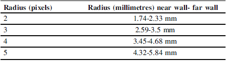
In this experiment our goal was to find the smallest possible radius that provides an accurate temperature measurement for PDT—small enough to be precise, but large enough to avoid interference from radiant heat emitted by the nozzle. To determine this, we start with the smallest radius and printed a test rectangle (Figure 3(a)), then incrementally increased the radius and repeated the process. We compared the results to identify the radius (Table 1) beyond which the nozzle’s radiation no longer influences the measurement. We saved the data for all the radius to different printing advances. Figure 3(b) shows the different height of the record.
Pixel radius correspondence in mm

In our code, the radius is defined in pixels around the hottest point. Table 1 shows the millimetre equivalents for the radii used. To establish this conversion, we measured the rectangle’s actual length and its length in pixels. The two values correspond to the radius equivalent for the nearest wall and the farthest wall, respectively. Due to perspective distortion, these walls do not have the same length in pixels.
3. Results
This section reports how the hottest-point tracking performs in practice and how measurement choices affect the recorded temperatures.
3.1. Visual observations of the hottest point method
Figure 5 shows the visual output of our system in multiple scenarios. All examples are obtained using the hottest point method described in Section 2.1.2. Figure 7(a) and (d) show scenarios where the temperature output is not saved as the point of measurement is blocked by the printhead. Visually, this correlates to when the green dot on the circle circumference is within the blue points. Figure 7(b) and (e) show scenarios where data is saved because the temperature output is correctly represented as the PDT. Figure 7(c) and (f) illustrate cases where the printer is moving without depositing material. In these situations, the hottest point is not the nozzle. Currently, these data points are manually removed from the dataset.
Result of the printing at different moments

3.2. Distance to object
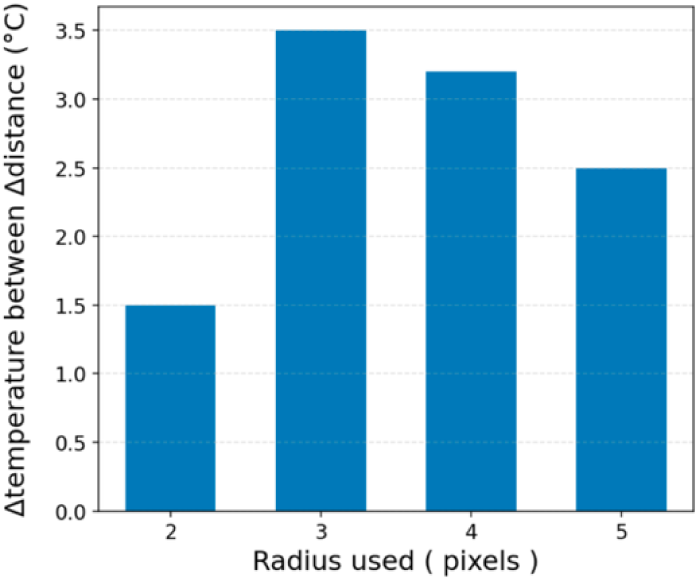
To evaluate potential limitations regarding camera-to-object distance we compared temperature readings from the nearest and farthest points during Experiment 1, with a distance difference (Δd) of 73 mm. As illustrated in Figure 6, the results show an average difference of 2 °C between the various radii, with 3 mm radius showing the largest difference of 3.5 °C. Radius 2 is the most consistent with a difference of only 1.5 °C. Although there is a measurable difference between the different radii and distances, the variation is only a few degrees. Therefore, we conclude that the distance between the measured point and the camera does not significantly affect the temperature measurements.
Influence of the distance on the results

The maximum deviation of observed for the 3-pixel radius can be attributed to the spatial resolution and perspective of the thermal camera. At 180 mm from the object, the physical area covered by a single pixel increases between the near wall and the far wall due to perspective distortion. However, as this variation remains close to the camera’s nominal accuracy of ± 2°C, it is concluded that the monitoring system can be reliably used across the entire print volume without the need for constant distance recalibration. This stability ensures that the PDT is captured consistently regardless of the nozzle’s position on the build plate.
3.3. Temperature monitoring of component
We conducted our experiment to identify the smallest possible radius used for thermal monitoring.
Figure 7 shows the plot for the different records.
PDT for different radii; samples from (a) the lower layer, (b) the middle layer and (c) the top layer

Across all three frame intervals, the temperature trends vary significantly depending on the selected radius. For radius 2, the temperature signal is highly unstable, exhibiting numerous sharp spikes. In Figure 7(a), the temperature fluctuates between approximately 50 °C and 90 °C; in Figure 7(b) it reaches values up to 105 °C; and in Figure 7(c) it ranges from 50 °C to about 75 °C. These large variations indicate that the radius 2 measurement is strongly influenced by the thermal radiation of the nozzle and does not provide reliable temperature information. For radius 3, the temperature generally remains within a narrower range of about 50–60 °C in Figures 7(a) and 7(b), suggesting a more consistent behaviour. However, in Figure 7(c), the temperature occasionally drops to values between 42 °C and 55 °C, showing that this radius is still susceptible to local fluctuations. For radius 4, the temperature curve is overall more stable, particularly in the first part of Figure 7(a), although isolated spikes still occur. A similar trend is observed in Figure 7(c), where the measurements remain smoother than for smaller radii but continue to exhibit occasional peaks. For radius 5, the measurements show more frequent and more pronounced spikes than radius 4, indicating that increasing the radius beyond 4 does not necessarily improve stability and may introduce additional noise into the measurement.
To evaluate the result, we also calculate the RMSE (Root Mean Squared Error of the values relative to 0, for each set of data. Table 2 shows the results.
Mean deviation for each radius

Table 2 summarises the RMSE values obtained for each radius. From R = 3 pixels onward, the RMSE does not change significantly. The relative differences between radii highlight this trend clearly: the RMSE decreases by 15.6 % when going from R2 to R3, but only by 3 % between R3 and R4, and a negligible 0.45 % between R4 and R5.
These results indicate a large improvement between R2 and R3, after which the measurements stabilize. Beyond R = 3 pixels, the variations become insignificant, suggesting that increasing the radius further does not provide meaningful benefits in terms of measurement accuracy.
4. Discussion
In this work, we developed a complete workflow for thermal monitoring during the 3D printing process. We designed and implemented a Python-based program capable of processing thermal camera data, filtering relevant information, and identifying the hottest point corresponding to the nozzle. The analysis allowed us to determine the smallest radius that provides temperature measurements close to the nozzle without being affected by its thermal radiation. Overall, this study demonstrates that combining thermal imaging with data processing and OpenCV provides a reliable tool for analysing and optimizing the thermal behaviour of the printing process.
We have identified that R3 provide the best accuracy as the difference between R3 and R4 is 1.52 °C, or 3%. When increasing the radius to R5 we risk losing details when monitoring, therefore the difference of only 1.5 °C to 0.23 °C when comparting R3 to R4 and R5 are negligible. The difference from R2 to R5 (best to worst) is 9.5 °C, or 20%. When comparing the radii we were able to identify the closest point to object as R3 (2.59-3.5 mm). When analyzing the radius effect on thermal monitoring, spikes in temperature were observed regularly for R2. In the layer closest to the bed, the temperature spikes upwards. We believe that this is caused by too few pixels as the number of pixels is constant between R2-R5, and when the printer is vibrating, the bed is captured instead of the PDT. In subsequent layers, the opposite effect was observed, strengthening our hypothesis, as vibrations here will either then cause recording of lower levels at lower temperatures, or the back of the printer also with a low temperature. A higher number of pixels will increase accuracy, but the aim of this paper is to get as close as possible to the nozzle, therefore this was not further investigated.
The machine-learning approach needs further work. We now know which colormap yields the most accurate results for the model. During development, we extracted frames from a video at 192x256 resolution (the same quality as manual snapshots taken with the code). At this resolution, the nozzle appears poorly defined in the images. A viable next step would be to annotate higher-quality images and use the appropriate colormap before training. We should also use more different angles on our dataset.
In the current implementation, the circle radius is set in pixels. A valuable change would be to express the radius in millimetres: calibrate the camera view once at the beginning, then apply the best radius directly in physical units. This would also allow non-integer equivalents (e.g., a pixel radius of 3.5) to be handled naturally when working in millimetres. Additionally, the number of sample points on the circle is fixed. For larger pixel radii, this can create gaps between sampled pixels; allowing a non-constant number of points a would maintain consistent spatial coverage. We can further improve the code by adding an additional condition to control whether the temperature data should be saved. Specifically, if the recorded temperature is located outside the printed part, its data should not be saved. In addition, we should exclude data collected when the printer is moving without printing. In such cases, the printer moves at a higher speed, which can easily be detected. Therefore, we can introduce a criterion based on the printer’s speed: if the speed exceeds a defined threshold, the temperature data should be neglected.
Finally, with the hottest-point method, we should mask parts of the printer body to reduce false detections. Applying low-emissivity tape (e.g., standard adhesive tape) or similar coverings can reduce spurious hotspots and improve localization. Thanks to the temperature data collected for each layer, we can now explore the relationship between the thermal history of the printed part and its resulting mechanical properties — for instance, how the temperature of the previous layer affects the local Young’s modulus or residual stresses. This approach provides a new parameter that can be integrated into process optimization and material modelling, allowing a better understanding of how printing conditions influence part performance.
Now that we have developed and validated the code, it can be implemented to monitor the temperature in high-temperature printing systems. However, the thermal camera used in this study operates only between 0 °C and 60 °C. To adapt it for use in such environments, certain modifications to the printer setup are necessary. Indeed, one of the next goals is to use the code with a high temperature material-extrusion 3D printer designed for high-performance polymers such as PEEK and PEI. For example, with the Orion printer (Germany, Berlin, Orion Additive Manufacturing GmbH), we considered removing a small section of the front glass panel to position the camera outside the heated chamber while maintaining a clear view of the print bed. Such an adaptation would extend the applicability of our monitoring system to a wider range of industrial 3D printers.
Integrating real-time thermal monitoring with mechanical analysis opens new opportunities for process control and design optimization. By correlating temperature distribution with mechanical performance, engineers can refine printing parameters, improve part reliability, and predict potential defects before they occur. This approach contributes to faster prototyping and more reliable production, ultimately accelerating the transition from experimental design to industrial-scale additive manufacturing.
5. Conclusion
This study presents a low-cost, in-situ temperature monitoring approach for capturing Pre Deposition layer Temperature in MEX AM. The method uses a Python-based workflow that combines thermal imaging with OpenCV to track the hottest point, corresponding to the printer nozzle. Experimental findings showed that using a 3-pixel radius (approximately 2.6–3.5 mm) for capturing the thermal data offered an optimal balance between minimizing variability from the nozzle radiation spikes and preserving spatial accuracy.
By enabling direct capture of thermal history during the fabrication process, this method provides critical process data that determines interlayer mechanical properties. Unlike machine-learning approaches that require extensive datasets and retraining for different setups, the hottest-point tracking method is robust and printer-independent, provided that the nozzle is the hottest point and remains visible during printing. Although validated on a desktop printer using PLA, the approach can be adapted to high-temperature systems and high-performance polymers, where thermal history is critical for part performance, predictive modelling, and ultimately certification.







 Open access

