2.1 ASKAP and the EMU survey

ASKAP is operated by the Commonwealth Scientific and Industrial Research Organisation (CSIRO) at the Inyarrimanha Ilgari Bundara, the CSIRO Murchison Radio-astronomy Observatory, in Western Australia. It consists of 36 $\times$ 12 m diameter radio antennas which are separated by baselines ranging from 37 m to 6 km resulting in angular scales of 10 $^{\prime\prime}$ – 3 $^\prime$ at frequencies from 700 to 1 800 MHz. All but six of the antennas are within a region of 2.3 km diameter, with the outer 6 extending the baselines up to 6 km. In the observations described here, as many of the 36 antennas were used as possible. However, in some cases a few antennas were omitted because of maintenance or hardware issues.

At the prime focus of each antenna is a Phased Array Feed (PAF), which subtends a solid angle of about 30 square degrees of the sky. The PAF consists of 192 single-polarisation dipole receivers. A weighted sum of the outputs of groups of these receivers is used to form 36 dual-polarisation ‘beams’, which together cover an area of about 30 square degrees. A full description of ASKAP may be found in Hotan et al. (Reference Hotan2021).

The two largest projects for which ASKAP was designed were EMU (Norris et al. Reference Norris2011; Hopkins et al. Reference Hopkins2025) and WALLABY (Koribalski et al. Reference Koribalski2020). Here we use data from the EMU-PS1 survey of EMU. The EMU-PS1 field was observed with ASKAP at a central frequency of 944 MHz, in the period 15 July to 24 November 2019. The observations and data processing are fully described by Norris et al. (Reference Norris2021a) so here we give only a brief overview. The data were taken in 10 tiles, covering 270 deg $^{2}$ , and taking a total of about 100 h of observing time. Here we use the ‘native’ resolution product, giving a synthesised beam of about $11 \times 13$ arcsec with an rms sensitivity of about 25 $\unicode{x03BC}$ Jy/beam.

2.2 Source extraction and characterisation

We have found (e.g. Boyce et al. Reference Boyce2023) that traditional automated source extractors such as Selavy (Whiting & Humphreys Reference Whiting and Humphreys2012) and PyBDSF (Mohan & Rafferty Reference Mohan and Rafferty2015) are relatively insensitive to extended structures, so no automated source extraction was used in this work. Instead, the sources were identified by visual inspection. We acknowledge that this may introduce its own bias and subjectivity. Our primary goal is to compile a catalogue of DRAGNs, so we ignore unresolved sources, and include other complex sources only if we think they may contain a DRAGN.

We first displayed the radio images on a large screen using CARTA (Comrie et al. Reference Comrie2018), using a linear transfer function, and setting the greyscale level so the 3- $\sigma$ noise peaks were just visible (see right-hand panel of Figure 1), and setting the spatial scale so an area of 10 $\times$ 20 arcmin was displayed on the screen. We then searched the image by eye, in three stages, for sources that appeared to be DRAGNs, as follows:

• • We first performed a careful visual raster scan through the entire radio image using CARTA, starting from the top left corner, moving across and down in a zig-zag pattern to the bottom right, identifying candidate sources, as shown in Figure 1.

• • For each source, we drew a rectangular ‘region’ around the source, whose position angle was matched, where possible, to the position angle of the jets. The major axis of the rectangle was adjusted visually to bound the lowest visible emission of the source, which corresponds roughly to the $5\,\sigma$ rms noise level of the image. Because the Gaussian image of a point source increases in size with source strength, this will result in a relatively larger box for strong sources, particularly FR2 sources in which the peak is close to the edge of the bounding box.

• • The third stage is to repeat the scan, focusing on finding any sources that might have been missed (i.e. are not marked by a rectangular region in the CARTA display) or whose total extent may have been under-estimated due to extended low-level emission. This last step was repeated several times by three different members of the author team (RPN, MY, and NG) until we were satisfied that no major sources had been missed. Our goal in doing so was to maximise the number of DRAGN-like sources larger than one arcmin, rather than prioritising any particular morphology.

• • For each source consisting of two lobes, we also measured the distance a between the maxima (identified visually) either side, using CARTA’s ‘Distance Measurement’ tool, for use in the FR1/FR2 classification, as described in Section 4.

• • For each source identified, we recorded the parameters of the region (centroid RA and Declination, major and minor axes b and c, and position angle). This RA and Declination is used to form the Identification (ID) of the source in Table 7. The parameter b is often called the “Largest Angular Size” in the literature.

• • For each source, we recorded an initial classification based on the morphology (e.g. FR1, bent-tail, X-shaped) and any further comments on the appearance (e.g. ‘overlaps with nearby source’).

These three stages resulted in the identification of a total of about 4000 candidate DRAGNs. During subsequent steps of this project (host identification, etc.), a few more sources were also found and added to the catalogue, while some sources were removed. We also identified and corrected any duplications, errors, and mis-classifications made in earlier stages. Our final list (hereafter referred to as ‘our catalogue’) of DRAGN candidates contains 3 557 sources.

2.3 Completeness

As the sources are identified by eye, this process is necessarily subjective and our catalogue of sources should not be considered a complete sample. Instead, the sources listed in this paper should be regarded as a representative, but substantially complete, sample of the sources in the image. We discuss the actual distribution of sizes and flux densities in Section 4.

While we clearly cannot detect sources that are below our sensitivity limit, we note that spatial filtering of the sources, as described by Rudnick (Reference Rudnick2002), can effectively increase the sensitivity of the data to low-surface brightness sources. A further exploration of this filtering, and the availability of python scripts to execute it, are found in Duchesne et al. (Reference Duchesne2024). Using this technique, we find several low-surface brightness sources in each of the 10 pointings that were not detected in our initial manual search. One of these is shown in Figure 2. Another radio galaxy (J204837.7-491145) with low-surface-brightness lobes is bright enough to appear in our catalogue, and is shown in Figure 23 of Norris et al. (Reference Norris2021a). That example is a remnant radio galaxy (e.g. Brienza et al. Reference Brienza2017), which is a galaxy in which the AGN has turned off, leaving two remnant radio lobes of aging electrons. Fainter examples may be identified using filtering, but are not sufficiently obvious in the full resolution images to be included in our catalogue. This is a conscious decision, implemented to maintain the consistency of our selection criteria.

Figure 2.

An example of a faint low-surface-brightness source that is not easily visible in the raw data but becomes obvious after spatial filtering, as described in Section 2.3. Left: raw unfiltered data. Right: filtered data. Although both lobes have some compact emission which is visible in the unfiltered EMU image, they appear as two disconnected compact sources and so were not included in our catalogue. Filtering reveals a radio galaxy with two connected low surface brightness lobes characteristic of aging electrons. Such sources that are visible only after spatial filtering are not included in our catalogue.

3.1 Identify the likely position of the host in the radio image

For DRAGNs that have a radio core we expect the host should coincide, or be very close to, the radio core (e.g. Gordon et al. Reference Gordon2023). In sources with a jet connected to the lobes, the host should lie on the line of the jet (e.g. Barkus et al. Reference Barkus2022). In double sources, the host often (but not always) lies roughly on the major axis of the source (or emission ridge), and is roughly equidistant from the two lobes. In sources with lobes of unequal brightness, the core tends to be closer to the brighter lobe (e.g. Mackay Reference Mackay1971; de la Rosa Valdés & Andernach Reference de la Rosa Valdés and Andernach2019).

3.2 Identify the host in the WISE images

We use the unWISE data release 6 images (Meisner, Lang, & Schlegel Reference Meisner, Lang and Schlegel2017; Meisner et al. Reference Meisner, Lang, Schlafly and Schlegel2019) which are derived from coadds of the WISE images over 5 yr, covering the entire sky at 3.4 and 4.6 $\unicode{x03BC}$ m, giving an angular resolution of $6.1^{\prime\prime}$ and $6.4^{\prime\prime}$ , respectively. They include the images from the NEOWISE phase of the WISE mission, resulting in five times the exposure time of the coadds from the initial WISE survey.

Having identified likely positions of the host in the radio image, we cross-matched the radio images with the unWISE images by visual inspection, by displaying two linked images in CARTA. In each case we then searched for an infrared (IR) source close to the expected host position. Our priority was reliability rather than completeness. In cases where no likely host was found in the IR image, we then re-examined the radio image to find likely positions of the host in the radio image that coincided with likely IR candidates.

If no plausible host was found, or our ability to find one was impacted by confusion or a nearby bright star, we do not associate the radio source with a host.

3.3 Identify the host in the CATWISE2020 catalogue

We matched the position of the IR source, measured from the unWISE (Schlafly, Meisner, & Green Reference Schlafly, Meisner and Green2019) image, with a source in the CATWISE2020 catalogue (Marocco et al. Reference Marocco2020) which is deeper and more reliable than the earlier unWISE catalogues. The cross-matching was done using the match function in TopCat (Taylor Reference Taylor, Shopbell, Britton and Ebert2005). To determine an appropriate search radius, we measured the number of cross-matches between the manually determined WISE IR hosts and the CATWISE2020 catalogue as a function of separation. We also estimated the false-ID rate by shifting the radio declination positions by 1 arcmin and then repeating the cross-match.

As a result, we adopted a maximum search radius of 2.0 arcsec, at which we get a 3.2% false-ID rate and a 90.0% total cross-match rate.

3.4 Summary of host identifications

The resulting numbers of sources are listed in Table 1, and the identifications themselves are listed in Table 7.

Table 1.

Numbers of sources remaining after each stage of the host identification of EMU-PS1 data.

Table 2.

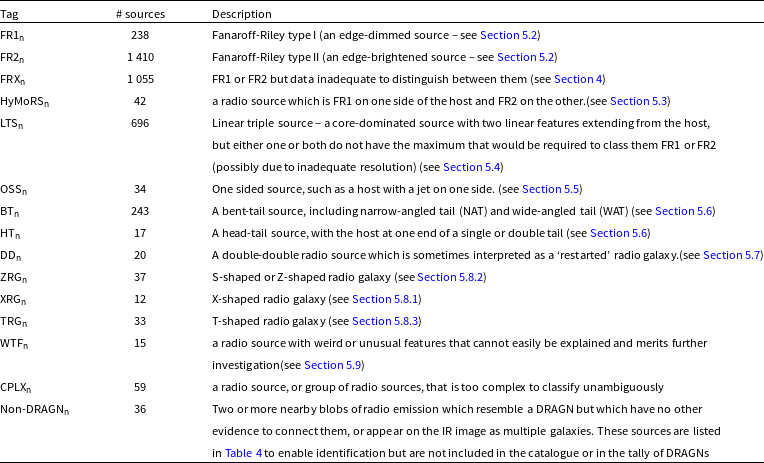
Tags used to classify sources. A source may have more than one tag, in which case it will appear in more than one row in this table. Tags are appended with the subscript $_{\rm n}$ as discussed in Section 1.3. The total number of DRAGNs includes all tagged sources except Non-DRAGNs.

3.5 Caveats

Because our source extraction and host identification processes are largely subjective, we stress that these results should be regarded as tentative, and subject to revision.

For example, to cross-match the initial manual identification of the IR host in the unWISE image to the CATWISE Survey has a quantifiable false-ID rate discussed above. However, we have no way of accurately estimating a false-ID rate of the initial match of the radio source to the IR sources visible in the unWISE image. Even when two different authors repeat the host identification, they are likely to be subject to the same biases and preconceptions. Our best guess, based on the number of sources which had an obvious host ID, compared to those where it was uncertain, suggest that our false-ID rate is likely to be about 10%.

It should also be emphasised that the above description may suggest that the source extraction, classification, and host identification processes occurred in a linear sequence. However, at each stage, earlier decisions were revisited, new sources were added to the catalogue, and some sources were dropped (e.g. when an apparent FR2 turned out during the host identification process to be two nearby interacting galaxies).

We plan to revisit the host identification in Paper IV of this series, where we will use all available multi-wavelength data to aid in the initial host identification, including higher-resolution radio data where available, and assign a reliability score to each host identification.

5.1 Classification process

Each source was inspected by eye and initially assigned one or more of the tags shown in Table 2, based primarily on radio morphology. This classification was subsequently revised (a) by using an algorithm, described below, to determine the FR1/FR2 classification, and (b) by taking into account the position of the host in the host identification step, such as a candidate FR2 source which turns out to be two (presumably interacting) galaxies with a connecting bridge of emission.

In the initial classification, there were four further tags that are not shown in Table 2:

• • Out of field: Part of the source lies beyond the outer boundary of the EMU-PS1 field

• • Artefact: The source appeared to be dominated by an imaging artefact

• • Single: The source appears to be a single component with no significant extension

• • Error: All other errors including human errors

Sources tagged with any of these four tags have not been included in the results shown in this paper. Every source in Table 7 has at least one of the tags shown in Table 2, and the mean number of tags/source is 1.15.

We note that these morphological tags are, of course, based on the two-dimensional projection of one or more three-dimensional objects, and it is possible that some unusual morphological shapes may be due to a projection of (e.g.) a bent-tail galaxy, or the superposition of two or more unrelated objects.

5.2 The Fanaroff-Riley classification

Fanaroff & Riley (Reference Fanaroff and Riley1974) showed that a selection of radio-loud AGNs could be classified into two morphological types: Fanaroff-Riley Class I (FR1) and Fanaroff-Riley Class II (FR2), according to the position of the brightness peaks of the radio emission, although the cause of the difference between the edge-brightened FR2 and the edge-dimmed FR1 is still unclear. FR2 jets seem to remain relativistic along their length until they abruptly end in a hotspot. FR1 jets, on the other hand, gradually decelerate along their length (e.g. Bicknell Reference Bicknell1995; Laing & Bridle Reference Laing and Bridle2002; Tchekhovskoy & Bromberg Reference Tchekhovskoy and Bromberg2016), as shown in Figure 4.

Figure 4.

Classifying a source as FR1 $_{\rm n}$ or FR2 $_{\rm n}$ relies on the measurement of a (the distance between the peaks) and b (the total extent of the source). FR1 $_{\rm n}$ have $a/b\lt0.5$ and FR2 $_{\rm n}$ have $a/b \gt 0.5$ . The top image satisfies the FR1 $_{\rm n}$ criterion ( $a/b \lt 0.5)$ , and the centre image satisfies the FR2 $_{\rm n}$ criterion ( $a/b \gt 0.5)$ . The bottom image satisfies the FR1 $_{\rm n}$ criterion ( $a/b \lt 0.5)$ but the small size combined with the measurement uncertainty makes the classification uncertain. We label such borderline cases as FRX $_{\rm n}$ , as described in Section 4. All distances are in arcsec.

Factors determining whether a source is FR1 or FR2 may include:

• • environmental effects, in which the jet loses energy through its interaction with the external medium, which will depend on external density(Bicknell Reference Bicknell1986; Bicknell Reference Bicknell1995; Kaiser & Best Reference Kaiser and Best2007). These effects include the entrainment or mass loading of a jet (Dekel & Birnboim Reference Dekel and Birnboim2006; Bicknell Reference Bicknell1995; Gopal-Krishna & Wiita 2001; Krause et al. Reference Krause, Alexander, Riley and Hopton2012; Perucho & Mart Reference Perucho and Mart2007; Perucho et al. Reference Perucho, Mart, Laing and Hardee2014).

• • the intrinsic properties of the accretion and jet formation processes near the parent Supermassive Black Hole (SMBH). Possible causes include the different content of the jet plasma (electron–positron pairs or normal electron–proton plasma), and the black hole spin (Reynolds et al. Reference Reynolds, Fabian, Celotti and Rees1996; Baum, Zirbel, & O’Dea Reference Baum, Zirbel and O’Dea1995; Meier Reference Meier1999).

Ledlow & Owen (Reference Ledlow and Owen1996) found that the FR1/II luminosity break depends on host-galaxy absolute magnitude, so that FR1s are found to have higher radio luminosities in more luminous host galaxies (where the density of the Interstellar Medium (ISM) is assumed to be higher). However, this result is based on highly flux-limited samples, with different redshift distributions and environments for the FR1s and FR2s. Therefore, the result does not necessarily apply to the broader population of radio galaxies (e.g. Best Reference Best2009; Wing & Blanton Reference Wing and Blanton2011; Shabala Reference Shabala2018). Furthermore, Krause et al. (Reference Krause, Alexander, Riley and Hopton2012) argued that FR1 sources must have previously passed through an FR2 phase, which precludes a fundamental difference based on the host galaxy.

In this paper, we adopt the original Fanaroff-Riley (FR) definition, as illustrated by Figure 4, which classifies sources based on the ratio $a/b$ of a (the distance between the brightest regions on opposite sides of the central host galaxy) to b (the total extent of the source). The measurement of a and b is described in Section 2.2. Sources with $a/b$ $\lt$ 0.5 are classified as the edge-darkened FR1 $_{\rm n}$ , while those with $a/b$ $\gt$ 0.5 are classified as the edge-brightened FR2 $_{\rm n}$ . In this project, a and b were measured as part of the Source Extraction and Characterisation process, as described in Section 2.2.

When measuring this ratio, Fanaroff & Riley say ‘The sources are classified using the ratio of the distance between the regions of highest brightness on opposite sides of the central galaxy or quasar; any compact component situated on the central galaxy was not taken into account’. This definition is open to some interpretation, as it does not, for example, specify how compact a central source must be to be excluded. We adopt an interpretation that excludes any central maximum (i.e. coincident with the host galaxy) from this classification, and base the classification only on the distance between the strongest maxima either side of the host galaxy. If there are no maxima either side of the core (or a maximum on only one side), then we do not classify it as an FR source, but as a linear triple source (LTS $_{\rm n}$ ).

Other authors may adopt different interpretations. For example, Figure 2(a) of Mingo et al. (Reference Mingo2019) is classified by them as a ‘lobed FR1’, because of the strong central source, whereas we would classify it as a core-dominated FR2, because the only maxima other than the central compact core are in the outer lobes, which thus satisfy the Fanaroff & Riley (Reference Fanaroff and Riley1974) definition of an FR2.

Such differences in classification criteria make it difficult to compare results from different surveys. In this paper we try to mitigate this problem by (a) explicitly defining our classification criteria, and (b) using tags, as discussed in Section 1.3, so that a definition can be traced back to the originating publication. We discuss this further in Section 6.4.

In some cases, a source is clearly double, and yet its small extent, compared to the resolution and measurement accuracy of the data, makes it difficult to determine whether it is FR1 $_{\rm n}$ or FR2 $_{\rm n}$ . We label such sources FRX $_{\rm n}$ . We introduce two parameters, $b_{\min}$ and $\epsilon$ , to quantify this uncertainty. We define $b_{\min}$ as the minimum value of b at which a measurement is meaningful, and $\epsilon$ as the uncertainty in the measurement of b.

We conducted experiments, using both real and simulated sources, to find the optimum value of these parameters. As a result, we adopt the values of $b_{\min}$ = 50 $^{\prime\prime}$ and $\epsilon$ = 10 $^{\prime\prime}$ .

The FR definition then becomes:

FR1 $_{\rm n}$ : $a/(b - \epsilon$ ) < 0.5 AND $b \gt b_{\min}$

FR2 $_{\rm n}$ : $a/(b + \epsilon$ ) > 0.5 AND $b \gt b_{\min}$

FRX $_{\rm n}$ : $a/(b + \epsilon) \lt 0.5 \lt a/(b - \epsilon$ ) OR $b \lt b_{\min}$

Throughout this paper, we use the term ‘FR sources’ to mean a source which is one of FR1 $_{\rm n}$ , FR2 $_{\rm n}$ , or FRX $_{\rm n}$ .

Given that FR1 sources tend to be less luminous than FR2 sources, it might be expected that the high sensitivity of EMU would find a larger number of FR1 sources than the earlier less sensitive surveys, but that is not the case. In our sample, we find many more FR2 $_{\rm n}$ than FR1 $_{\rm n}$ sources. We discuss this later in Section 6.

Figure 3 also shows that FR II $_{\rm n}$ dominate the larger sources, with their size distribution peaking at $\sim 100^{\prime\prime}$ compared to $\sim 50^{\prime\prime}$ for other morphologies. However, the flux density distribution of the FR1 $_{\rm n}$ differs from other morphologies, peaking at $\sim 50\,$ mJy, in comparison to $\lesssim 10\,$ mJy for the rest of the DRAGNs. A discussion of the implications of this for the physics of FR1 and FR2 must await Paper IV where we derive source luminosities.

5.3 HyMoRS $_{\rm n}$

Hybrid morphology sources (HyMoRS) are a rare type of radio source that satisfy the FR1 criteria on one side of their host galaxy, and the FR2 criteria on the other side. Here they are tagged as #HyMoRS $_{\rm n}$ and not #FR1 $_{\rm n}$ or #FR2 $_{\rm n}$ .

They were first identified as a class by Gopal-Krishna & Wiita (2000). Kapińska et al. (2017) found 25 new candidate HYbrid MOrphology Radio Sources (HyMoRS) using Radio Galaxy Zoo (Wong et al. Reference Wong2025). Since then several other authors have listed larger samples of HyMoRS (e.g. Kumari & Pal Reference Kumari and Pal2022). We find that 42 of our 3 557 radio sources are HyMoRS $_{\rm n}$ candidates, or slightly more than 1% of DRAGNs. Alternatively, HyMoRS $_{\rm n}$ represent about 2.6% of all FR sources (FR1 $_{\rm n}$ +FR2 $_{\rm n}$ +HyMoRS $_{\rm n}$ ), where we exclude FRX $_{\rm n}$ because we would not be able to detect HyMoRS $_{\rm n}$ morphology in that group. This may be compared with the results of Gawroński et al. (2006) who estimated that $\lesssim$ 1% of a sample of strong extended radio sources are HyMoRS. This suggests that HyMoRS may be more common in fainter samples of radio sources.

HyMoRS provide potentially important clues to understanding the FR1/FR2 dichotomy. For example, intrinsic effects like the black hole spin must be common to both sides, so the very existence of HyMoRS favours an environmental cause for the FR1/FR2 dichotomy (Gopal-Krishna & Wiita 2000; Gopal-Krishna & Wiita 2002). This support for environmental causes has been reinforced by high-resolution observations (Harwood, Vernstrom, & Stroe Reference Harwood, Vernstrom and Stroe2020) and modelling (Stroe et al. Reference Stroe, Catlett, Harwood, Vernstrom and Mingo2022).

Figure 5 shows a few examples of the HyMoRS sources in our sample, as follows.

Figure 5.

Examples of HyMoRS $_{\rm n}$ sources, which appear to be FR1 on one side and FR2 on the other. In these and all subsequent multi-panel Figures, the white box is the rectangular region bounding box described in Section 2.2 and the red cross is the tentative position of the host. If no cross is shown, then we were unable to identify a host.

J201556.3-583648 resembles a double-double source (see Section 5.7, with each side having an inner and outer lobe, but in the northern arm the inner lobe is brighter than the outer, while in the south the outer is brighter than the inner.

J202051.7-552745 is a classic example of a HyMoRS $_{\rm n}$ , with the southern jet being very clearly edge-brightened, while the northern jet gradually fades over its length.

In J202714.3-531401 the southern lobes is a classic edge-brightened FR2 lobe, while the northern lobe peaks a short distance from the core, and then gradually fades.

J213717.4-540544 has a bright hot-spot in the east, while the western jet is a thin bending arc which fades over its length.

J213917.3-541936 resembles a classic FR2, except for the hotspot half-way down its southern jet which is brighter than the hotspot, thus converting it from an FR2 $_{\rm n}$ to a HyMoRS $_{\rm n}$ .

J215826.9-583502 has a classic FR2 hot spot terminating its northern jet, while the southern jet reaches a peak a short distance from the core and then fades over its length, although both jets have a similar shape.

While these few examples on their own cannot add significantly to the FR1/FR2 debate, EMU-PS1 contains 42 HyMoRS $_{\rm n}$ candidates, so that the whole EMU survey will contain thousands of such objects, which are likely to have a significant influence on our understanding of the FR dichotomy.

5.4 Linear triple sources (LTS $_{\rm n}$ )

LTS $_{\rm n}$ sources are core-dominated sources that have two linear features extending from the host, but either one or both features do not have the maximum that would enable them to be classified as FR1 $_{\rm n}$ or FR2 $_{\rm n}$ .

We find 696 of these sources, a sample of which are shown in Figure 6. It is possible that in higher resolution observations, some might show a maximum near the core that would qualify them as FR1 $_{\rm n}$ . Alternatively, they could be high-redshift FR2 sources where the lobes have been diminished by inverse Compton losses (Turner & Shabala Reference Turner and Shabala2020). In either case, they still represent a distinct morphological class. To the best of our knowledge, this class has not previously been identified in the literature, although they are probably similar to the ‘naked jets’ identified by Parma et al. (Reference Parma, Fanti, Fanti, Morganti and de Ruiter1987) and de Ruiter et al. (Reference de Ruiter, Parma, Fanti and Fanti1990). The large number found in this survey, and their relative absence in earlier surveys, suggests they they are largely confined to the low-luminosity end of the distribution of AGN.

Figure 6.

Examples of LTS $_{\rm n}$ (Linear triple) sources which have two jets but lack the maxima on both sides that would enable them to be classified as a FR source. The source J203135.0-592022, is very asymmetrical and has a curious 90 $^{\circ}$ bend in one jet.

Several of the sources in Figure 6 show slight bending of the jets. In the most extreme case, J203135.0-592022, the north-west jet executes an abrupt 90 $^{\circ}$ bend shortly after leaving the core.

5.5 One-sided sources (OSS $_{\rm n}$ )

OSS $_{\rm n}$ are sources that, in the EMU images, have a jet on one side of the host but no detectable jet can be seen on the other.

The vast majority of DRAGNs are two-sided, but a significant minority, including the very first radio-loud quasar to be identified, 3C273, have one-sided jets. The jet in 3C273 is observed at radio, optical, and X-ray wavelengths and no counter-jet has ever been detected (Courvoisier Reference Courvoisier1998). One-sided jets are relatively common in radio-loud quasars, and are presumably due to relativistic boosting of the nearside jet (Kellermann & Owen Reference Kellermann, Owen, Kellermann and Verschuur1988).

Also relatively common are double-lobed sources in which the jet is one-sided at small scales, but then becomes two-sided at kpc scales, presumably as the jet loses energy and becomes sub-relativistic, so that relativistic beaming is seen only near the core (Kellermann & Owen Reference Kellermann, Owen, Kellermann and Verschuur1988). Such one-sided jets at Very Long Baseline Array (VLBI) scales are often called core-jet sources (e.g. Yang et al. Reference Yang2021).

Much rarer are sources, corresponding to our OSS $_{\rm n}$ class, in which the emission at kpc scales is one-sided. Nevertheless, a significant number has been catalogued over the years (Kapahi Reference Kapahi1981; Saikia et al. Reference Saikia, Shastri, Cornwell, Salter, Swarup and Kapahi1986; Saikia et al. Reference Saikia, Junor, Muxlow and Tzioumis1989; Saikia et al. Reference Saikia, Junor, Cornwell, Muxlow and Shastri1990; Saikia et al. Reference Saikia, Thomasson, Jackson, Salter and Junor1996).

At this scale, in most cases the jet is unlikely to be relativistic, and so the one-sidedness may be attributed to an intrinsically one-sided source, possibly because the source ‘flip-flops’ between the two sides (van Groningen, Miley, & Norman Reference van Groningen, Miley and Norman1980; Laing et al. Reference Laing, Parma, de Ruiter and Fanti1999; Rudnick & Edgar Reference Rudnick and Edgar1984; Kellermann & Owen Reference Kellermann, Owen, Kellermann and Verschuur1988).

In our sample, we found 34 candidate one-sided sources. Some have a suggestion of a counter-jet that is much shorter than the main jet, suggesting that these are very asymmetric sources rather than true one-sided sources. Furthermore, to establish that a source is a genuine one-sided source, the position of the host needs to be determined. We show a sample of those that have a host galaxy coincident with the putative core in Figure 7. In two sources, J204111.4-613953 and J215424.7-545208, the jet bends sharply after leaving the core, presumably due to the effect of intergalactic gas. At least two sources (J211335.7-571639 and J204111.4-613953) have a suggestion of a counter-jet.

Figure 7.

Examples of candidate OSS $_{\rm n}$ (one-sided) sources. Many show a bent tail, notably J204111.4-613953 and J215424.7-545208 which have a 90 $^{\circ}$ bend in the jet close to the host, possibly due to a superposition of sources.

Figure 8.

Examples of BT $_{\rm n}$ (bent-tail) sources.

5.6 Bent-tail and head-tail sources (BT $_{\rm n}$ , HT $_{\rm n}$ )

In the majority of DRAGNs, the two jets/lobes and the host galaxy are roughly in a straight line. In a significant minority, the two jets are bent, presumably by their interaction with the intergalactic medium.

In this paper we tag any DRAGN where the jet is bent by more than 10 $^{\circ}$ (i.e. so the angle between the jets must be less than 170 $^{\circ}$ ) as a ‘Bent-tail’ (BT $_{\rm n}$ ) source.

BT $_{\rm n}$ sources are often divided into three subsets:

• • Wide-Angle Tail sources (WATs): Sources in which the angle between the two jets is greater than 90 $^{\circ}$ . We note that some authors do not include this bending angle in their criterion for a WAT (e.g. Missaglia et al. Reference Missaglia2019).

• • Narrow-Angle Tail sources (NATs): Sources in which the angle between the two jets is less than 90 $^{\circ}$

• • Head-tail (HT) sources. Sources in which the tails are bent around so far they they end up parallel, and frequently combine so that only one tail is seen at the largest scales or in low resolution observations.

In this paper we do not attempt to tag sources with NAT or WAT (since the classification often changes with distance from the host), but we do identify the HT $_{\rm n}$ class.

These definitions are not universally adopted, which leads to much confusion in the literature. For example, the HT source was first recognised by Ryle & Windram (Reference Ryle and Windram1968), although they did not actually use the term. The term ‘head-tail’ was first used by Miley et al. (Reference Miley, Perola, van der Kruit and van der Laan1972), and a clear definition was first given by Mao et al. (Reference Mao, Johnston-Hollitt, Stevens and Wotherspoon2009) as follows: Head–tail (HT) sources are a subclass of radio galaxy whose radio jets are distorted such that they appear to bend in a common direction. This gives rise to the so-called ‘HT’ morphology where the radio jets are bent back to resemble a tail with the luminous galaxy as the ‘head’. Here we adopt this definition.

Most authors (including those cited above) effectively define the HT label in the same way (e.g. Rudnick & Owen Reference Rudnick and Owen1976), but we note that some authors (e.g. Sasmal et al. Reference Sasmal, Bera, Pal and Mondal2022b; Pal & Kumari Reference Pal and Kumari2023) adopt a definition of HT to include all bent-tail sources, even WATs. For example, none of the sources in the catalogue of 55 HT sources listed by Pal & Kumari (Reference Pal and Kumari2023) would be recognised as an HT by the Miley or Mao definitions. To some extent this problem can be circumvented by the use of subscripted tags (see Section 1.3) but we would still urge authors to avoid confusion by using widely adopted definitions where possible.

We show a sample of BT $_{\rm n}$ sources in Figure 8. They show a variety of morphologies. In most cases (e.g. J201055.5-530851, J202921.5-494441, J220947.2-553451) it is easy to understand the source in terms of the conventional explanation that the source is moving with respect to the intergalactic medium, and that the jet leaves the source with enough energy to withstand the ram pressure, but as it loses energy the jet is blown back by the intergalactic medium. However, two cases (J201852.9-525523 and J214827.1-571149) have such tangled morphologies that a more complex mechanism must be invoked. For example, perhaps the source is immersed in an intergalactic medium with a complex turbulent motion such that the direction of flow varies rapidly along the length of the jet, or perhaps the host galaxy is orbiting a companion (e.g. Blandford & Icke Reference Blandford and Icke1978).

Bent-tail sources were first found when studying the radio emission from clusters (Ryle & Windram Reference Ryle and Windram1968; Miley et al. Reference Miley, Perola, van der Kruit and van der Laan1972), and they have since traditionally been viewed as tracers of clusters (e.g. Owen & Rudnick Reference Owen and Rudnick1976; Rudnick & Owen Reference Rudnick and Owen1976; Giacintucci & Venturi Reference Giacintucci and Venturi2009; Lao et al. Reference Lao2025). Their relationship to clusters will be explored in Paper III of this series.

5.6.1 HT $_{\rm n}$ candidates

HT sources are DRAGNs in which the two jets have been bent round to form a single tail. We show a sample of candidate HT $_{\rm n}$ sources in Figure 9. We call them ‘candidate’ HT $_{\rm n}$ sources to acknowledge that the identification of these sources is rarely unambiguous, and some may be alternatively identified as one-sided sources (OSS $_{\rm n}$ ).

Figure 9.

Examples of HT $_{\rm n}$ (head-tail) candidate sources, in which the two jets from the SMBH appear to have curved round to form a single tail.

To confirm that they really are HT $_{\rm n}$ sources would require high-resolution observations to test whether, close to the head, there really are two jets which are then curved around.

5.6.2 Bending as a function of FR1 $_{\rm n}$ and FR2 $_{\rm n}$ class

If FR1 sources have lower jet powers than FR2 sources, then it might be expected that FR1 sources are more easily bent by the ram pressure of intergalactic gas, and so we might expect BT sources to be more prevalent amongst FR1 sources than FR2 sources. This is largely borne out by observations. For example, Barnes (Reference Barnes2025) find that in a sample of 72 sources drawn from the 3CRR survey (Laing, Riley, & Longair Reference Laing, Riley and Longair1983), 23.6% of 3CRR FR2 sources and 70.6% of 3CRR FR1 sources are bent by more than 30 $^{\circ}$ , so that, in that admittedly small sample, an FR1 source is almost four times more likely to be bent than an FR2.

In Table 3 we show that, in our sample, while a greater fraction of FR1 $_{\rm n}$ sources are bent than FR2 $_{\rm n}$ , the fraction of bent FR1 $_{\rm n}$ sources is less than twice that of FR2 $_{\rm n}$ sources. Furthermore, the fraction of either that are bent is lower than in brighter samples. This will be explored further in Paper III of this series.

Table 3.

Frequency of BT $_{\rm n}$ sources as a function of FR1 $_{\rm n}$ /FR2 $_{\rm n}$ classification.

5.7 Double-double radio sources (DD $_{\rm n}$ )

A ‘double-double’ (or DD) radio source is defined by Schoenmakers et al. (Reference Schoenmakers, de Bruyn, Röttgering, van der Laan and Kaiser2000) as ‘a pair of double radio sources with a common centre’. Implicit in their definition is that the two sources must also have a common axis. They qualify this definition by adding ‘Furthermore, the two lobes of the inner radio source must have a clearly extended, edge-brightened radio morphology’ which confines DD sources to FR2 sources. Here we relax this latter criterion to admit the possibility that DD sources may include FR1 sources. However, we must also be careful to distinguish a true DD source from a double source that simply has strong symmetrical knots in its jets, and so add the clause that each of the double radio sources must have the morphology of a normal FR radio source.

We have also found examples, shown in Figure 10, in which there are three or more double radio sources. These were first identified by Brocksopp et al. (Reference Brocksopp, Kaiser, Schoenmakers and de Bruyn2007) and more have since been found (e.g. Dabhade et al. Reference Dabhade, Chavan, Saikia, Oei and Rottgering2024). Rather than creating more subclasses, we include these in the category of DD $_{\rm n}$ sources. We therefore end up with a revised definition of a double-double source, as ‘two or more double radio sources with a common centre and a common axis, each of which has the morphology of a normal FR radio source.’

Figure 10.

Examples of double-double (DD $_{\rm n}$ ) sources, sometimes called ‘restarted sources’, in which there appears to be a pair of older diffuse lobes surrounding a younger inner double radio source. Sometimes there are more than two ‘generations’ of radio lobes.

It is now widely accepted that DD sources are caused by an AGN first generating the outer lobes, then switching off and switching on again to generate the inner lobes. They are thus also often called ‘restarted’ radio sources (Schoenmakers et al. Reference Schoenmakers, de Bruyn, Röttgering, van der Laan and Kaiser2000; Mahatma et al. Reference Mahatma2019; Saikia, Konar, & Kulkarni Reference Saikia, Konar and Kulkarni2006). In this case we can, in principle, learn much about AGN duty cycles by studying DD sources. An alternative model is that the lobes result from jet-cloud interactions (Young et al. Reference Young, Turner, Shabala, Stewart and Yates-Jones2024).

In or catalogue we find 20 DD $_{\rm n}$ sources, a sample of which are shown in Figure 10. Of these 20 DD $_{\rm n}$ sources, 14 have two lobes on each side, one (J210542.7-571912) has three lobes on each side, two (J201404.8-522628, J202817.8-492419) have an unequal number of lobes on each side, and one (J214401.1-563712; see Figure 14) has a ‘trident’ morphology which we discuss further in Section 5.9.

5.8 Winged radio sources (XRG $_{\rm n}$ , ZRG $_{\rm n}$ , TRG $_{\rm n}$ )

Winged radio sources are sources which have one or more linear structures extending from the side of the major axis of the main radio source. Here we identify three types of winged sources:

• • X-shaped radio galaxies, or XRG $_{\rm n}$ , which have two linear structures emanating from the source to give the radio source the appearance of the letter ‘X’, as shown in Figure 11.

  Figure 11.

  Examples of XRG $_{\rm n}$ (X-shaped radio galaxies).

  

• • S/Z-shaped radio galaxies, or ZRG $_{\rm n}$ , which have two linear structures emanating from opposite sides of the lobes, giving the radio source the appearance of the letter ‘S’ or ‘Z’, as shown in Figure 12

  Figure 12.

  Examples of ZRG $_{\rm n}$ (S- and Z- shaped radio galaxies).

  

• • T-shaped radio galaxies, or TRG $_{\rm n}$ , which have one or more linear structures emanating from the side of the source, giving the radio source the appearance of the letter ‘T’,‘L’, or ‘M’as shown in Figure 13

  Figure 13.

  Examples of TRG $_{\rm n}$ (T-shaped radio galaxies) with linear extensions emanating from the side of the source. J210704.7-501143 differs from the others in that the protrusions are diffuse, suggesting a different mechanism operating in this case.

  

5.8.4 Mechanisms driving winged radio sources

We recognise that all these three different morphologies are similar except for the location of the linear protrusion(s).

We also acknowledge that, with all such peculiar radio morphologies, in some cases the protrusion might be caused by the superposition of two unrelated sources, or be a projection effect, but this is unlikely to be the cause in most cases.

Although we have identified these three different types of morphology, we are not asserting that they are produced by different mechanisms, and it is possible that just one mechanism (e.g. backflow, as suggested by Cotton et al. (Reference Cotton2020) for XRG), is responsible for all these morphologies. That backflow may then burst out of the radio galaxy at different points, depending on the local conditions. Further studies will be required to establish whether this is the cause.

Figure 14.

Examples of WTF $_{\rm n}$ sources, discussed in Section 5.9.

Figure 15.

Two examples of CPLX $_{\rm n}$ sources that are too complex to classify as a DRAGN.

We also note the similarities between the winged morphologies and the ‘Trident’ morphologies discussed below in Section 5.9.

5.9 Unusual sources (WTF $_{\rm n}$ )

With the advent of large radio surveys with with millions of sources, probing parts of parameter space that have never before been observed, it was recognised several years ago that new types of radio source were almost certain to be found (Norris Reference Norris2017a), including ones with surprising morphologies that do not easily fit into the known classes of radio source. Norris (Reference Norris2017a) coined the name WTF (for ‘Widefield ouTlier Finder’) to describe these objects, which we now adopt as a tag to describe such objects.

The first WTF sources to be found in the EMU survey were the Odd Radio Circles (ORCs) (Norris et al. Reference Norris2021b). Although it lies in the EMU-PS1 field covered by our catalogue, ORC 1 does not appear in our catalogue because it does not resemble a DRAGN. However, ORCs 2 and 3 do appear in our catalogue as they do indeed contain a DRAGN, which is now thought to be the causes of ORC2 and 3 (Macgregor et al. Reference Macgregor2025), unlike the other ORCs which are thought to be caused by a shock from the elliptical galaxy at their centre (Norris et al. Reference Norris2021b; Koribalski & et al. Reference Koribalski2025).

We find 15 such WTF $_{\rm n}$ objects in our catalogue that defy description in conventional terms, and we show a sample of them in Figure 14. It should be remembered in all cases that the two-dimensional appearance may be misleading. For example, apparently abrupt changes in jet direction may result from modest changes in a foreshortened jet seen end-on.

J214331.8-510534, which we call “The Trident”, appears to have emission along the edge of a cavity, possibly tracing a backflow. The extension of the core to the west is due to an unresolved background source. We note that Knowles et al. (Reference Knowles2022) found a very similar source in the cluster MCXC J2104.9-8243.

J214401.1-563712 shows traces of a similar morphology with a flattened triple structure at each end, but without the backflows seen in the first source. The extensions to the side of the source are perhaps related to the winged sources described in Section 5.8.

J205850.2-573648 is the source ORC2/3, first found by Norris et al. (Reference Norris2021b) and discussed in detail by Macgregor et al. (Reference Macgregor2025).

J220026.4-561051 was identified as an ORC candidate by Gupta et al. (Reference Gupta2022) but may be a BT source.

J203243.2-515249 is a very asymmetric source with a long jet on one side and a diffuse blob on the other. It could perhaps be described as a HyMoRS $_{\rm n}$ (see 5.3) but that does not do justice to its extreme asymmetry.

J201923.4-565139 is also an asymmetrical source, which could be classified as a ‘double-double’ or a WAT, but the interesting feature is that one lobe has a distinct circular appearance, perhaps explained by the ORC model of Shabala et al. (Reference Shabala2024).

J220713.7-580611 has two rings instead of lobes, also strongly suggesting the Shabala et al. (Reference Shabala2024) ORC mechanism.

We dub J212953.0-585824 the Mickey Mouse source. It may be two overlapping sources, or perhaps an extreme example of a T-shaped source. This source deserves further observations at higher resolution.

Similar collections of unusual objects have also been found in LOFAR data (Sasmal, Bera, & Mondal Reference Sasmal, Bera and Mondal2022a; Gopal-Krishna, Patra, & Joshi Reference Gopal-Krishna2025)

5.10 Complex sources

In some cases, we have been unable to classify a source because of its complex structure. Two examples are shown in Figure 15. One is the well-known ‘Dancing Ghosts’ source J213414.0-533637 (Norris et al. Reference Norris2021a) which has been discussed in detail by Velović et al. (2023). The other, J213518.9-620415, may be a combination of cluster emission together with the strong emission from a Brightest Cluster Galaxy (BCG). Both of these sources show filaments which are still poorly understood.

5.11 Non-DRAGN sources

36 sources consist of two or more nearby blobs of radio emission which resemble a DRAGN but which have no other evidence to connect them, or appear on the IR image as multiple galaxies. We list these in Table 4 for future reference. These sources are not included in the main catalogue or in the total number of DRAGNs. Two examples are shown in Figure 16.

Table 4.

Table of non-DRAGN sources that resemble DRAGNs.

6.1 3CRR

The 3CRR sample (Laing et al. Reference Laing, Riley and Longair1983) is a reliable catalogue of strong radio sources revised from the earlier 3CR survey (Bennett Reference Bennett1962). Table 1 shows that only 76% of the sources in our DRAGN catalogue are FR sources (i.e. FR1 $_{\rm n}$ , FR2 $_{\rm n}$ , or FRX $_{\rm n}$ ). The remaining sources have morphologies such as LTS $_{\rm n}$ , OSS $_{\rm n}$ , and HT $_{\rm n}$ which cannot be classified as FR sources. By comparison, at least 89% of the 181 3CRR strong radio sources listed in table 3 of Laing et al. (Reference Laing, Riley and Longair1983) are FR sources (the actual breakdown is 132 are FR2, 29 are FR1 and 20 are core-dominated sources). In this and other early catalogues focusing on strong sources, the other morphologies discussed in this paper (e.g. LTS, OSS) are virtually absent.

This illustrates a major difference between the early catalogues of strong sources and the current generation of large catalogues of much fainter sources: fainter sources show a much wider range of morphologies, and much more morphological disturbance, than the strong sources.

6.2 NVSS and FIRST

Gendre et al. (Reference Gendre, Best and Wall2010) compiled and classified a subset of sources from NVSS, which they call the CONFIG sample, and which should constitute a valuable comparison with our catalogue. Unfortunately, the value to us is reduced because their classification process is rather different from ours. For example, Gendre et al. included core-jet sources in the FR2 class, and HyMoRS sources were included in either FR1 or FR2 categories, depending on their most prominent features. CONFIG consists of four sub-samples with different areas and sensitivities, none of which are comparable with the survey here. Nevertheless, we summarise the morphological classifications of the total sample in Table 5.

The MiraBest sample (Porter & Scaife Reference Porter and Scaife2023; Miraghaei & Best Reference Miraghaei and Best2017) is a labelled sample of 1 256 low-redshift $(0.03 \lt z \lt 0.1)$ radio-loud AGN from NVSS and FIRST. which are limited to FR1, FR2, and Hybrid (corresponding to our HyMoRS $_{\rm n}$ ) morphologies. Here we reject those that are classified as ‘uncertain’, leaving 852 sources that they label as ‘confident’. We rearrange Table 2 of Porter & Scaife (Reference Porter and Scaife2023) and compare their results with ours in Table 5.

The sensitivities, resolutions, and areas covered by the surveys are too different to draw any physical significance from Table 5. For example, Figure 17 shows the Miraghaei & Best (Reference Miraghaei and Best2017) catalogue only covers the upper tip of the EMU-PS1 flux range because of the deeper EMU-PS1 data, but finds smaller DRAGNs because of the higher resolution of FIRST. However, two things are notable. First, the FR1/FR2 ratio of our catalogue and CONFIG are similar, but both are much higher than the MiraBest catalogue. It is unclear why this should be, given that CONFIG and MiraBest are drawn from the same data, but is a useful illustration of the hazards of comparing catalogues made with different selection criteria. Second, the fractions of BT, HT, DD, and HyMoRS in our catalogue and MiraBest are comparable (i.e. within a factor of about two).

6.3 VLASS

The Karl G. Jansky Very Large Array (VLA) Sky Survey (VLASS; Lacy et al. Reference Lacy2020) is a multi-epoch survey of the entire sky north of -40 $^{\circ}$ at $\sim$ 3 GHz at high resolution. The first epoch of VLASS was completed in 2019 (Gordon et al. Reference Gordon2021), and Quick Look images covering $\sim$ 34 000 deg $^2$ are publicly available.

Figure 16.

Two examples of non-DRAGN sources that were initially classified as a DRAGN from their radio appearance, but the IR images show that each radio component is probably a separate galaxy.

Figure 17.

A comparison of the size-flux space occupied by DRAGNs identified by EMU in this work (solid grey), by NVSS and FIRST (Miraghaei & Best Reference Miraghaei and Best2017, blue), LoTSS DR1 (Mingo et al. Reference Mingo2019, red), and VLASS (Gordon et al. Reference Gordon2023, yellow). The contour levels contain $95\,$ %, $67\,$ %, $33\,$ %, and $5\,$ % of the distributions. The flux densities from other surveys are extrapolated to the EMU frequency of $944\,$ MHz assuming a spectral index of $\alpha=-0.7$ . Each of the surveys is at a different frequency, so comparing them tells us about the frequency dependence of the DRAGN population.

Gordon et al. (Reference Gordon2023) searched the VLASS Quick-look images for DRAGNs using an algorithm they called DRAGNhunter, and identified 17 724 DRAGNs. A detailed comparison of their data with ours is complex because the two surveys differ so greatly in observing frequency, resolution, and sensitivity. At a higher frequency than EMU, VLASS at $3\,$ GHz may be more biased towards identifying DRAGNs with bright hotspots or younger radio lobes. VLASS was observed using the VLA in BnA configuration, a setup that lacks the short baselines needed to detect radio structures larger than a few tens of arcseconds across. A consequence of this, for example, is that while two hotspots of a large FR II may be identifiable in VLASS, large and diffuse FR Is are likely missing from the Gordon et al. (Reference Gordon2023) catalogue. The point source sensitivity of VLASS is substantially lower than that of EMU, with a typical rms noise in VLASS of $130\,\unicode{x03BC}\text{Jy}\,\text{beam}^{-1}$ . For objects with a typical spectral index of $\alpha=-0.7$ , the faintest point sources in VLASS ( $S_{3\,\text{GHz}}\sim 0.65\,$ mJy) would appear to be $\sim 1.5\,$ mJy in EMU, approximately 15 times brighter than the faintest objects in EMU. This results in a much lower source density for VLASS (0.51 deg $^{-2}$ ) than for our survey (13.11 deg $^{-2}$ ). The effects of these differences are seen clearly in Figure 17, where the DRAGNs identified in this work (grey shading) occupy an almost totally different region of the angular size/flux density plane to the DRAGNs identified by Gordon et al. (Reference Gordon2023), yellow contours.

6.4 LoTSS

The LoTSS survey (Shimwell et al. Reference Shimwell2017, Reference Shimwell2019) at 144 MHz has a median sensitivity of 71 $\unicode{x03BC}$ Jy/beam and a resolution of 6 $^{\prime\prime}$ . Assuming a spectral index $\alpha = -0.7$ , this is equivalent to a sensitivity of 19 $\unicode{x03BC}$ Jy/beam at 944 MHz, which is comparable to that of EMU-PS1. A catalogue of double sources, based on LoTSS, similar to that presented here, has been published by Mingo et al. (Reference Mingo2019), with the primary goal of studying the FR dichotomy. Of all the catalogues discussed here, this is the most similar to ours, and so comparisons might in principle yield information about the differences between sources selected at 944 MHz and those selected at 144 MHz.

Table 5.

Comparison of our tags with the MiraBest and CONFIG samples. In each case, a source may be assigned more than one tag.

Table 6.

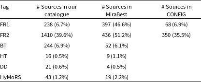
Comparison of FR1/FR2 sources from our paper and Mingo et al. (Reference Mingo2019), limited to FR/LTS sources with size $\gt 60^{\prime\prime}$ (i.e. S2 class in Mingo et al. Reference Mingo2019) and $S_{150}\gt50\,$ mJy, $S_{944}\gt13.4\,$ mJy (i.e. F3 class in Mingo et al. Reference Mingo2019).

Figure 17 shows that the DRAGNs in LoTSS occupy a similar location in size/flux space but differs in two respects: (1) LoTSS finds a population of smaller DRAGNs that our survey misses, because of their higher resolution, (2) our survey finds larger DRAGNs at low-flux densities than LoTSS, possibly because of better sensitivity to low surface brightness emission by EMU-PS1, or differences in methodology. We note that the newer LOTSS DR2 (Shimwell et al. Reference Shimwell2022) has greater low surface brightness sensitivity than the LOTSS DR1 survey used by Mingo et al. (Reference Mingo2019).

Mingo et al. (Reference Mingo2019) used the sample of 23 344 radio-loud sources with optical/IR identifications and redshifts listed by Hardcastle et al. (Reference Hardcastle2019). They further restricted the sample to those with a size > 12 $^{\prime\prime}$ and S $_{150}$ >2 mJy, and further reliability filtering, to obtain a catalogue of 5 805 radio sources. Their sample is therefore a factor of 5 805/3 557 = 1.6 larger than ours.

They then applied a combination of automated classification and visual checking, to obtain samples of FR1, FR2, and other classifications. Here we refer to their classifications using the tags FR1 $_{\rm m}$ and FR2 $_{\rm m}$ .

Comparing the results from Mingo et al. (Reference Mingo2019) with those in this paper suffers from a number of challenges, which are illustrated by Table 6, in which we show a comparison of the numbers of FR1/FR2 sources found by morphological type. Here we have used the numbers from Table 3 of Mingo et al. and restricted it to their class S2 (size $\gt 60^{\prime\prime}$ ) and F3 (total flux $\gt 50\,$ mJy). We apply the same criteria to our data, scaling the total flux limit to S $_{944\,{\rm MHz}}$ >13.4 mJy, assuming a spectral index of $\alpha = -0.7$ . The two samples should thus be similar, other than the observing frequency.

It is clear there is a major difference, with Mingo et al seeing far more FR1 $_{\rm m}$ than FR2 $_{\rm m}$ , while we see far more FR2 $_{\rm n}$ than FR1 $_{\rm n}$ . In addition to any astrophysical reason for this, we can identify six main effects that would lead to this difference.

First, we note that, as discussed in Section 5.2, Mingo et al. adopted a definition of an FR1 $_{\rm m}$ which includes the radio emission associated with the host galaxy, whereas our definition of an FR1 $_{\rm n}$ depends only on the maxima of the extended radio jets/lobes, and ignores any central radio emission associated with the host galaxy. For example, we would classify as an FR2 $_{\rm n}$ the example of an FR1 $_{\rm m}$ source given in Figure 2(a) of their paper.

Second, we recognise a class of sources (FRX $_{\rm n}$ ) for which we would say the classification is uncertain, whereas all sources in Mingo et al. are classified as FR1 $_{\rm m}$ or FR2 $_{\rm m}$ . Their confidence in their classification was helped by the higher resolution of the LoTSS data compared to EMU data, but some marginal classifications are presumably included in their counts of FR1 $_{\rm m}$ and FR2 $_{\rm m}$ .

Third, we recognise a category of source (LTS $_{\rm n}$ , or Linear triple source, discussed further in Section 5.4) in which two jets are seen, but either one or both do not have maxima that would enable them to be classified as FR sources. These would also be classified by Mingo et al. as FR1 $_{\rm m}$ .

Fourth, hotspots tend to be flatter spectrum than the diffuse jet or lobe emission of an FR2 (e.g. Treichel et al. Reference Treichel, Rudnick, Hardcastle and Leahy2001; Mahatma et al. Reference Mahatma2020), so they are less prominent at low frequencies. Thus, even with the same number of beams across the source, at low frequencies, the separation of the emission peaks will be closer together than at high frequencies. This becomes even more important when coupled with the increase in beam size at low frequency; it can cause a source that is clearly FR2 at higher frequencies to appear as an FR1 at low frequencies, as shown in Figure 18.

Figure 18.

A cartoon simulation of an FR2 source consisting of two rectangular “jets” or “lobes”, $10''\times 50''$ , separated by 50”, with spectral index $\alpha = -1.5$ . At the outer end of each jet/lobe is a hotspot consisting of a 5” circular Gaussian with spectral index $\alpha = -0.7$ . The model at each observing frequency (150 and 1 500 MHz) is shown at the bottom, with the flatter spectrum hot spots indicated by magenta lines. Their contrast against the steep spectrum jets/lobes is much lower at 150 MHz. At the top, the observations at a resolution of $30^{\prime\prime}$ , (5 beams across the source), are shown. The double-sided arrows indicate the observed separation between peaks, as used in the FR1/II definition. In this example, the peaks are $150^{\prime\prime}$ apart in the model, but observed to be $143^{\prime\prime}$ , and $108^{\prime\prime}$ apart in the 1 500 and 150 MHz observations, respectively.

Fifth, Mingo et al. used an automated approach that is likely to produce a higher error rate for individual objects and may misclassify the most unusual objects, although it does have the advantage of being immediately scalable to larger survey areas. However, we note that for large strong sources used here (categories S2 and F3), their reliability appears to be high (84% for FR1 $_{\rm m}$ and 94% for FR2 $_{\rm m}$ ) and so this should not be a major factor.

Sixth, the Mingo et al. catalogue is restricted to sources with an optical/IR identification, which will tend to bias it to lower redshift and lower excitation sources compared to ours. However, since Mingo et al. include sources even if they only have a WISE identification, and since 90% of our sources do have a WISE identification (see Table 1), this will probably only have a small effect on the comparison.

These differences may help explain why Mingo et al. see many more FR1’s than we do, and why we find many more FR2’s than they do. These differences will be explored further in Paper IV.