

1. Introduction
How do environmental regulations affect where firms choose to invest across borders? This question lies at the intersection of two major policy debates: the environmental consequences of globalization and the effectiveness of regulatory frameworks in shaping firm behavior. While a large body of work has examined the environmental implications of trade liberalization and globalization (Copeland and Taylor, Reference Copeland and Taylor2004; Cherniwchan et al. Reference Cherniwchan, Copeland and Taylor2017; Cherniwchan and Taylor, Reference Cherniwchan and Taylor2022), significant uncertainty remains regarding the role of environmental policy stringency in influencing foreign direct investment (FDI).
Two competing hypotheses dominate this debate. The “Porter Hypothesis” (PH) (Porter, Reference Porter1991; Porter and Linde, Reference Porter and v. d. Linde1995) argues that stringent environmental regulations foster innovation, leading to productivity gains and long-term competitiveness. In contrast, the “Pollution Haven Hypothesis” (PHH) (Copeland and Taylor, Reference Copeland and Taylor2000) posits that firms shift investment toward countries with laxer environmental standards to minimize compliance costs. This dynamic may be exacerbated by globalization, which, through declining transport and communication costs, has lowered relocation barriers even for less footloose industries (Kellenberg, Reference Kellenberg2009). As Cherniwchan et al. (Reference Cherniwchan, Copeland and Taylor2017) emphasize, such relocation may contribute to the lack of global convergence in environmental outcomes and the breakdown of the Environmental Kuznets Curve (EKC) (Grossman and Krueger, Reference Grossman and Krueger1991).
This paper contributes new evidence to this debate by constructing a novel, cross-country measure of environmental policy stringency and assessing its impact on bilateral FDI stocks. We develop the Environmental Stringency Index (ESI), an original indicator that captures both policy implementation and regulatory commitment, and can be applied consistently across 111 countries. Unlike existing proxies, such as abatement costs or emissions intensities, the ESI avoids problems of endogeneity and limited comparability. It enables us to empirically examine the extent to which firms reallocate capital in response to differences in environmental policy across countries.
To do so, we combine the ESI with bilateral FDI data from Broner et al. (Reference Broner, Didier, Schmukler and von Peter2023) and estimate an augmented structural gravity model of FDI using the Poisson Pseudo-Maximum Likelihood (PPML) estimator. Our dataset spans 111 source and 121 host economies over the period 2001-2018. The analysis focuses on the effects of environmental stringency in host countries, as well as the absolute difference in stringency between source and host countries, capturing potential regulatory arbitrage.
Our findings provide robust support for the PHH. Stricter environmental regulations in host countries are associated with significantly lower levels of inward FDI. This effect is particularly pronounced for emerging economies, while it is weaker and less robust for high-income countries. Moreover, we show that FDI responds not only to the stringency level in the host country but also to the regulatory gap between source and host economies. Specifically, the negative effect of stringent regulation is amplified when the difference in regulatory intensity across countries is larger, suggesting that firms are actively responding to cross-border differences in environmental costs.
This paper makes several key contributions. First, we introduce a novel, cross-country index of environmental policy stringency that addresses the limitations of widely used proxies. While abatement costs suffer from poor international comparability, and emissions-based measures are potentially endogenous to firm location decisions, our index captures both de jure and de facto aspects of environmental regulation and enables consistent cross-country analysis. Importantly, the ESI is designed to disentangle two core dimensions of environmental policy: implementation, which reflects the formal commitment and ambition of a country’s regulatory framework, and enforcement, which we operationalize as the degree to which actual emissions deviate from predicted levels, conditional on structural factors. This distinction allows us to go beyond existing indices, which often do not distinguish between the formal intent of environmental regulation and its actual effectiveness in practice. Our empirical findings indicate that investors are more responsive to the implementation component of regulation, interpreted as a credible signal of future regulatory costs, than to enforcement outcomes, which may be perceived as less predictable or less observable ex ante. Second, we provide new empirical evidence of the PHH using a rich panel of bilateral FDI stocks, estimated within a structural gravity framework that accounts for multilateral resistance and extensive fixed effects. Third, we document that the regulatory gap, i.e., the absolute difference in environmental stringency between source and host countries, plays a significant role in shaping investment stocks, suggesting that firms actively engage in regulatory arbitrage. Finally, we present heterogeneity analyses by host country income level and host country specialization in natural resources, showing that the PHH effect is particularly strong in emerging markets and not confined to traditionally resource-intensive industries.
The remainder of this paper is organized as follows. Section 2 reviews the relevant empirical literature. Section 3 introduces our novel regulatory indicator. In Section 4, we present the data used and outline the empirical model employed in this study. The main findings are discussed in Section 5. Robustness tests are conducted in Section 6. Finally, Section 7 offers conclusions and explores potential extensions to broaden the scope of our analysis.
2. Literature review
2.1. Cross-country evidence on the PHH
The empirical validity of the PHH remains widely debated. Early cross-country studies found limited support for the idea that environmental regulation significantly influences FDI flows, leading some to characterize the PHH as a “popular myth” (Javorcik and Wei, Reference Javorcik and Wei2003). These studies argued that environmental compliance costs are often marginal relative to total relocation costs, and that capital-intensive, polluting industries, typically a comparative advantage of developed economies, are less likely to relocate.
Seminal reviews by Jaffe et al. (Reference Jaffe, Peterson, Portney and Stavins1995) and empirical studies such as Eskeland and Harrison (Reference Eskeland and Harrison2003) reported weak or no evidence in favor of the PHH. Copeland et al. (Reference Copeland, Shapiro, Taylor, Copeland, Shapiro and Taylor2022) identify two core reasons for this: (i) endogeneity of environmental policy, where openness to trade can influence regulatory design (Ederington and Minier, Reference Ederington and Minier2003), and (ii) the absence of reliable, internationally comparable measures of policy stringency.
More recent work has produced mixed findings. While several studies find significant effects of environmental regulation on trade flows, the evidence on FDI remains inconclusive or context-specific (Copeland et al. Reference Copeland, Shapiro, Taylor, Copeland, Shapiro and Taylor2022). A growing number of papers exploit bilateral FDI data to uncover cross-country patterns. For instance, Naughton (Reference Naughton2014) finds that environmental regulation (proxied by emissions) deters inward FDI across OECD countries. However, emissions are endogenous to economic activity, complicating causal inference.
Many studies rely on country-specific or sub-national variation. Keller and Levinson (Reference Keller and Levinson2002) find a small deterrent effect of U.S. state-level abatement costs on inbound FDI. In China, Cai et al. (Reference Cai, Lu, Wu and Yu2016) exploit the Two Control Zones (TCZ) policy, showing that stricter air pollution rules reduced FDI inflows, especially from countries with weaker environmental standards. Yet such evidence is difficult to generalize, and cross-country conclusions remain limited by data comparability and identification challenges.
2.2. Firm- and industry-level evidence
At the micro level, firm- and industry-level studies provide richer behavioral insights, though findings remain heterogeneous. Industry-level research tends to support the PHH, particularly in pollution-intensive sectors. For example, Wagner and Timmins (Reference Wagner and Timmins2009) in Germany, Poelhekke and van der Ploeg (Reference Poelhekke and van der Ploeg2015) in the Netherlands, and Chung (Reference Chung2014) in South Korea all document relocation effects in response to stricter environmental policies.
Firm-level evidence, by contrast, is more mixed. Hanna (Reference Hanna2010) shows that the 1990 U.S. Clean Air Act Amendments led to increased foreign investment by U.S. multinationals. Similarly, Kheder and Zugravu (Reference Kheder and Zugravu2012) find strong PHH effects for French firms, with FDI directed away from countries with stricter policies, except in the Commonwealth of Independent States. Candau and Dienesch (Reference Candau and Dienesch2017) corroborate these findings for European firms. However, other studies, such as Raspiller and Riedinger (Reference Raspiller and Riedinger2008) (on French firms) and Manderson and Kneller (Reference Manderson and Kneller2012) (on U.K. firms), report no significant evidence of relocation due to environmental regulation.
Interestingly, a complementary strand of the literature has identified the opposite pattern: FDI attraction to jurisdictions with stricter environmental standards, explained by mechanisms such as the “Green Haven Effect,” “Race to the Top,” or “Pollution Halo” hypothesis (Kheder and Zugravu, Reference Kheder and Zugravu2012; Rivera and Oh, Reference Rivera and Oh2013; Poelhekke and van der Ploeg, Reference Poelhekke and van der Ploeg2015; Bialek and Weichenrieder, Reference Bialek and Weichenrieder2021). These frameworks argue that stronger environmental rules may signal institutional quality, attract cleaner technologies, or encourage innovation, aligning with the “Porter Hypothesis.”
Overall, the literature suggests substantial variation in FDI responses to environmental regulation, depending on country characteristics, sectoral composition, and measurement strategies. A key limitation of existing cross-country studies lies in their reliance on imperfect proxies for policy stringency, such as emissions levels or abatement costs, and the difficulty of separating policy intent from policy enforcement.
This paper contributes to this literature by introducing a novel index that distinguishes between implementation (policy commitment) and enforcement (actual compliance, measured as the gap between predicted and actual emissions). This enriches the analysis of Naughton (Reference Naughton2014) that only focuses on 22 countries and measure regulation using emission intensities. Indeed, this approach enables more credible identification of the PHH across a broad panel of countries. In doing so, we offer a comprehensive test of regulatory arbitrage in FDI decisions using a global bilateral dataset, while accounting for both absolute stringency and regulatory asymmetries between source and host countries.
3. A Novel indicator of stringency
In this section we introduce our new ESI and explain its unique features that differentiate it in the field of environmental assessment.
3.1. Limitations of previous environmental indicators
If the existing literature fails to draw uniform conclusions on the effect of environmental regulations on economic outcomes, it is mainly due to the use of different proxies to gauge environmental policies. Three primary methods have been employed in the literature (Cole et al. Reference Cole, Elliott and Zhang2017; Galeotti et al. Reference Galeotti, Salini and Verdolini2020). The predominant approach entails using abatement costs, such as data sourced from the Pollution Abatement Costs and Expenditure Survey in the U.S. (see Eskeland and Harrison, Reference Eskeland and Harrison2003; Keller and Levinson, Reference Keller and Levinson2002), to ascertain the regulatory pressures encountered by firms or industries. However, these measures are constrained by limited country and time coverage. Moreover, standardizing data on pollution abatement costs presents challenges, impeding their application to a panel of countries. Alternatively, some studies (see Xing and Kolstad, Reference Xing and Kolstad2002) rely on emissions or emissions intensities, though this introduces a simultaneity bias, as emissions can be both as a cause and a consequence of FDIs. Lastly, certain papers use the extent of environmental legislation, such as the U.S. Clean Air Act Amendments (see List et al. Reference List, McHone and Millimet2004; Hanna, Reference Hanna2010). Nonetheless, this approach is also constrained, as its coverage can be exceedingly limited and unsuitable for international comparisons. Given our objective of establishing an international measure of environmental policy stringency encompassing a diverse array of countries over time, we advocate for the adoption of an environmental regulation index. Although composite indicators have been used in prior literature (Dasgupta et al. Reference Dasgupta, Mody, Roy and Wheeler2001; Kruse et al. Reference Kruse, Dechezleprêtre, Saffar and Robert2022), they also encounter limitations, arising from limited temporal and country coverage.
In constructing the ESI, we aim to create an improved measure of environmental stringency that addresses all the issues highlighted by Galeotti et al. (Reference Galeotti, Salini and Verdolini2020). First of all, we tackle the multidimensionality issue considering a composite index that incorporates both the commitment and the enforcement of environmental regulations. Indeed, Brunel and Levinson (Reference Brunel and Levinson2013) assess that regulations are effective only if they are enforced, highlighting the need for both commitment and enforcement measures. To our knowledge, the only instrument that considers both aspects is the annual Executive Opinion Survey (Manderson and Kneller, Reference Manderson and Kneller2012; Mulatu, Reference Mulatu2017). However, it is essential to acknowledge that this survey-derived database inherently incorporates subjectivity, which could potentially impact the reliability of the measured levels of stringency and enforcement. In addition, we need to match the regulation to the policy issue being addressed. Since our focus is on reducing greenhouse gas emissions to mitigate global warming, we prioritize activities that contribute to emissions reduction and carbon removal.
Secondly, we tackle the simultaneity issue by adopting the methodology proposed by Brunel and Levinson (Reference Brunel and Levinson2013). They introduce a novel indicator that estimates the expected emissions for each jurisdiction by considering its industrial composition and the average emissions intensity of its industries. By employing this approach, we not only address the simultaneity issue but also overcome limitations associated with industrial composition. In countries where pollution-intensive industries are prevalent, there may be higher expenditures on pollution abatement measures. Relying solely on emissions intensity as a measure of environmental stringency can introduce bias, as it may incorrectly suggest that countries with higher emissions intensity are implementing more stringent environmental regulations. Lastly, we underscore the issue of data availability by creating an indicator that covers a broad range of countries, approximately 164, and considers both developed, developing, and emerging economies. Previous composite indexes, such as the Environmental Policy Stringency index ( $EPS$
) have notably neglected low-income economies, while they are known as the primary pollution havens.
$EPS$
) have notably neglected low-income economies, while they are known as the primary pollution havens.
3.2. Construction of the environmental stringency index
A dual dimension
In constructing the ESI, we focus on evaluating two crucial dimensions of environmental regulations. Firstly, we aim to quantify nations’ commitment to implementing environmental policies and fostering international cooperation. Secondly, we assess the effectiveness of enforcement mechanisms and the level of dedication toward achieving established objectives, especially those related to climate change mitigation. This focus directly stems from the status of climate change as one of the major challenges of the 21st century. The Paris Agreement (2015), which constitutes the primary action taken to address this challenge, urges countries to develop long-term strategies of low greenhouse gas emissions. Thus, by centering our indicator on climate change mitigation, we align with the goals of the Paris Agreement, making it a crucial tool for assessing countries’ progress in implementing environmental policies.
To collect the data, we rely on the University of Gothenburg’s Quality of Government Environmental Indicators Dataset (Povitkina et al. Reference Povitkina, Pachon and Dalli2021). This open resource includes various environmental indicators, such as policy presence, ecological footprint, level of emissions, and public sentiment.
Implementation
Our approach to policy implementation focuses on two key aspects, encompassing both national and international commitments to combat climate change. At the national level, we quantify the number of climate-related policies currently in place, drawing on the Climate change mitigation law or policy in place ( $CCL$
) variable (GRICCE and SCCCL, 2021). The legislative and policy landscape target the reduction of greenhouse gas emissions, employing various strategies such as emission limits, permit trading systems, and investment in cleaner technologies. Additionally, we consider legislation related to forests and land use if they specifically contribute to emission reduction and carbon capture efforts. On the international front, our analysis centers on International Environmental Agreements (
$CCL$
) variable (GRICCE and SCCCL, 2021). The legislative and policy landscape target the reduction of greenhouse gas emissions, employing various strategies such as emission limits, permit trading systems, and investment in cleaner technologies. Additionally, we consider legislation related to forests and land use if they specifically contribute to emission reduction and carbon capture efforts. On the international front, our analysis centers on International Environmental Agreements ( $IEA$
) specifically linked to climate change. Using data from the International Environmental Agreements Database Project, we construct a variable, ranging from 0 to 6, that captures whether a country has signed or ratified a selected set of six key agreements. Three of these agreements were initially used by Javorcik and Wei (Reference Javorcik and Wei2003), the Convention on Environmental Impact Assessment in a Transboundary Context, the Convention on Long-range Transboundary Air Pollution, and the Convention on the Transboundary Effects of Industrial Accidents. To reflect more recent developments, we also include the Paris Agreement, the Montreal Protocol on Substances that Deplete the Ozone Layer, and the United Nations Framework Convention on Climate Change (UNFCCC). All of these agreements collectively aim to mitigate climate change through diverse approaches. The Paris Agreement and the Montreal Protocol directly target greenhouse gas emissions and ozone-depleting substances, respectively, aligning with broader climate change mitigation goals. Similarly, the UNFCCC seeks to stabilize greenhouse gas concentrations in the atmosphere. Additionally, agreements addressing environmental impacts and industrial accidents indirectly support climate change mitigation by promoting sustainable development practices and reducing pollutants that contribute to global warming.
$IEA$
) specifically linked to climate change. Using data from the International Environmental Agreements Database Project, we construct a variable, ranging from 0 to 6, that captures whether a country has signed or ratified a selected set of six key agreements. Three of these agreements were initially used by Javorcik and Wei (Reference Javorcik and Wei2003), the Convention on Environmental Impact Assessment in a Transboundary Context, the Convention on Long-range Transboundary Air Pollution, and the Convention on the Transboundary Effects of Industrial Accidents. To reflect more recent developments, we also include the Paris Agreement, the Montreal Protocol on Substances that Deplete the Ozone Layer, and the United Nations Framework Convention on Climate Change (UNFCCC). All of these agreements collectively aim to mitigate climate change through diverse approaches. The Paris Agreement and the Montreal Protocol directly target greenhouse gas emissions and ozone-depleting substances, respectively, aligning with broader climate change mitigation goals. Similarly, the UNFCCC seeks to stabilize greenhouse gas concentrations in the atmosphere. Additionally, agreements addressing environmental impacts and industrial accidents indirectly support climate change mitigation by promoting sustainable development practices and reducing pollutants that contribute to global warming.
Enforcement
Regarding countries’ enforcement, we base our approach on the study by Brunel and Levinson (Reference Brunel and Levinson2013) and develop a country emissions-based indicator. We argue that the most effective way to measure a country’s abatement efforts is by examining their actions to reduce greenhouse gas emissions, as outlined in the Paris Agreement (2015). To that extent, we compute the enforcement aspect $Enf_{yt}$
as the ratio of predicted emissions intensity of country y (
$Enf_{yt}$
as the ratio of predicted emissions intensity of country y ( $\hat e_{yt}$
) to actual emissions intensity of country y at time t (
$\hat e_{yt}$
) to actual emissions intensity of country y at time t ( $e_{yt}$
) considering
$e_{yt}$
) considering $z$
sectors:
$z$
sectors:
 \begin{equation} Enf_{yt}=\frac {\hat e_{yt}}{e_{yt}} \quad {\rm with}\quad \hat e_{yt} = \sum _{z=1}^4 \frac {V_{yzt}}{V_{yt}} \frac {E_{zt}}{V_{zt}} \quad {\rm and}\quad e_{yt}=\frac {E_{yt}}{V_{yt}} \end{equation}
The actual emission intensity $e_{yt}$
reflects the total emissions
$e_{yt}$
reflects the total emissions $E_{yt}$
of country
$E_{yt}$
of country $y$
relative to its total value added
$y$
relative to its total value added $V_{yt}$
, serving as a measure of the emissions generated per unit of output. Conversely, the predicted emission intensity
$V_{yt}$
, serving as a measure of the emissions generated per unit of output. Conversely, the predicted emission intensity $\hat {e}_{yt}$
is computed as a weighted average of sector-specific emission intensities (
$\hat {e}_{yt}$
is computed as a weighted average of sector-specific emission intensities ( $\frac {E{zt}}{V_{zt}}$
), where the weights correspond to the sectoral composition of country
$\frac {E{zt}}{V_{zt}}$
), where the weights correspond to the sectoral composition of country $y$
, that is, the share of each sector
$y$
, that is, the share of each sector $z$
in the country’s total value added (
$z$
in the country’s total value added ( $\frac {V_{yzt}}{V_{yt}}$
). Countries exhibiting higher
$\frac {V_{yzt}}{V_{yt}}$
). Countries exhibiting higher $Enf_{yt}$
levels are regarded as stringent nations as
$Enf_{yt}$
levels are regarded as stringent nations as $\hat {e}_{yt} \gt e_{yt}$
suggests that the predicted emissions intensity within their industries exceeds their current emission intensity. It is a signal of pollution reduction efforts undertaken under stricter regulations. We source sectoral emissions data (
$\hat {e}_{yt} \gt e_{yt}$
suggests that the predicted emissions intensity within their industries exceeds their current emission intensity. It is a signal of pollution reduction efforts undertaken under stricter regulations. We source sectoral emissions data ( $E_{yzt}$
) from Climate Watch (Reference Watch2022), and sectoral value added (
$E_{yzt}$
) from Climate Watch (Reference Watch2022), and sectoral value added ( $V_{yzt}$
) from the United Nations database. To obtain country-level aggregates (
$V_{yzt}$
) from the United Nations database. To obtain country-level aggregates ( $E_{yt}$
,
$E_{yt}$
, $V_{yt}$
), we sum all sector values within each country while sector-level aggregates (
$V_{yt}$
), we sum all sector values within each country while sector-level aggregates ( $E_{zt}$
,
$E_{zt}$
, $V_{zt}$
) are derived by summing values across all countries for each sector. Sectors are grouped into four broad categoriesFootnote
1
to ensure consistency with emissions data. All monetary values are converted into U.S. dollars to allow cross-country comparability. Descriptive statistics for both the implementation and enforcement indices are presented in Table A1.
$V_{zt}$
) are derived by summing values across all countries for each sector. Sectors are grouped into four broad categoriesFootnote
1
to ensure consistency with emissions data. All monetary values are converted into U.S. dollars to allow cross-country comparability. Descriptive statistics for both the implementation and enforcement indices are presented in Table A1.
Z-score approach
Inspired by Kheder and Zugravu (Reference Kheder and Zugravu2012), who applied the Z-Score strategy to variables such as multilateral environmental agreements, international non-governmental organization and emission efficiency, we adopt a similar approach and standardize the data by calculating individual Z-scores for each of the three variables $s$
. This process involves subtracting the mean
$s$
. This process involves subtracting the mean $\mu _{st}$
from each data point (
$\mu _{st}$
from each data point ( $X_{jst}$
) and then dividing by the standard deviation
$X_{jst}$
) and then dividing by the standard deviation $\sigma _{st}$
, ensuring that the variables are on a comparable scale.
$\sigma _{st}$
, ensuring that the variables are on a comparable scale.
 \begin{equation} Z_{jst}=\frac {X_{jst} - \mu _{st}}{\sigma _{st}} \end{equation}
The Z-scores for the number of climate-related policies, international environmental agreements, and the enforcement component are then summed with equal weights to create a comprehensive Z-score index ranging from 0 to 100, with 100 representing the highest level of stringency.
Descriptive statistics
With a panel of more than 160 countries, our analysis reveals notable heterogeneity in environmental policy stringency across the globe, as shown on the world map in Figure 1. Darker shades signify more stringent environmental policies, particularly evident in regions such as Europe. North America similarly demonstrates a dedication to robust regulatory frameworks. In contrast, lighter shades predominate in numerous African nations, suggesting lower levels of stringency. Similar results regarding heterogeneity were observed in the first year under analysis, 2001, as documented in Figure A1.
Regarding the evolution over the past twenty years and considering the developmental stage of each country, Figure A2 indicates a global trend towards more stringent environmental regulations. Developed economies consistently demonstrate the highest levels of environmental stringency, beginning at around 30 in 2000 and steadily increasing to approximately 55 by 2020. In contrast, emerging and developing economies show a gradual rise in their mean ESI, but the gap between them and developed economies has widened over the study period.
Lastly, it is crucial to assess whether increases and disparities in environmental stringency are driven by implementation or enforcement. Figure A3 compares these aspects across countries for the year 2018. Developed nations, especially in Europe and America, exhibit higher adoption rates and enforcement of environmental measures. In contrast, developing countries encounter challenges in both implementing and adopting stricter environmental policies. These observations underscore a critical point: by examining both implementation and enforcement, we gain a more comprehensive understanding of environmental rigor and its implications.

Figure 1. ESI by country for 2018.
3.3 Environmental stringency index and previous indicators
To comprehensively evaluate the effectiveness of the $ESI$
in capturing the dynamics of environmental policies, we conducted an analysis to determine its correlation with previously employed indicators, survey-based metrics, and taxation measures. For composite indexes, we rely on the Environmental Performance Index (
$ESI$
in capturing the dynamics of environmental policies, we conducted an analysis to determine its correlation with previously employed indicators, survey-based metrics, and taxation measures. For composite indexes, we rely on the Environmental Performance Index ( $EPI$
) from the Yale Center (Block et al. Reference Block, Emerson, Esty, de Sherbinin and Wendling2024) and the Environmental Policy Stringency index (
$EPI$
) from the Yale Center (Block et al. Reference Block, Emerson, Esty, de Sherbinin and Wendling2024) and the Environmental Policy Stringency index ( $EPS$
) from the OECD (Kruse et al. Reference Kruse, Dechezleprêtre, Saffar and Robert2022). Regarding survey-based measurements and taxation variables, we respectively rely on a survey question, “To what extent are environmental concerns effectively taken into account?” (
$EPS$
) from the OECD (Kruse et al. Reference Kruse, Dechezleprêtre, Saffar and Robert2022). Regarding survey-based measurements and taxation variables, we respectively rely on a survey question, “To what extent are environmental concerns effectively taken into account?” ( $BTI$
) and policies pertaining to environmentally related tax revenue per capita (
$BTI$
) and policies pertaining to environmentally related tax revenue per capita ( $ERTR$
).
$ERTR$
).
Table 1 shows notable correlations between our $ESI$
and both the aggregate indicator
$ESI$
and both the aggregate indicator $EPS$
and the fiscal policy measure
$EPS$
and the fiscal policy measure $ERTR$
. However, the correlations with
$ERTR$
. However, the correlations with $EPI$
and
$EPI$
and $BTI$
are moderate, which can be explained by their specific focuses. On one hand, the
$BTI$
are moderate, which can be explained by their specific focuses. On one hand, the $EPI$
primarily assesses a country’s performance in addressing climate change, aligning more with enforcement efforts than implementation. This distinction will be explored further in our robustness tests to examine enforcement’s impact on FDI.Footnote
2
On the other hand, the moderate correlation with
$EPI$
primarily assesses a country’s performance in addressing climate change, aligning more with enforcement efforts than implementation. This distinction will be explored further in our robustness tests to examine enforcement’s impact on FDI.Footnote
2
On the other hand, the moderate correlation with $BTI$
is likely due to the subjective nature of its survey-based data. Importantly, the high correlation with
$BTI$
is likely due to the subjective nature of its survey-based data. Importantly, the high correlation with $EPS$
underscores the
$EPS$
underscores the $ESI$
’s robustness in comprehensively measuring environmental policy stringency. By creating the
$ESI$
’s robustness in comprehensively measuring environmental policy stringency. By creating the $ESI$
, we aimed to enhance the original
$ESI$
, we aimed to enhance the original $EPS$
by incorporating additional information that reflects a broader spectrum of environmental governance practices. Figure A4 highlights the inclusion of additional countriesFootnote
3
in the
$EPS$
by incorporating additional information that reflects a broader spectrum of environmental governance practices. Figure A4 highlights the inclusion of additional countriesFootnote
3
in the $ESI$
that were not covered by the
$ESI$
that were not covered by the $EPS$
. Referencing Figure 1, we observe that the
$EPS$
. Referencing Figure 1, we observe that the $EPS$
tended to overlook countries with less stringent environmental regulations. By including these countries in our analysis, we improve our ability to assess the relationship between FDI and environmental stringency.
$EPS$
tended to overlook countries with less stringent environmental regulations. By including these countries in our analysis, we improve our ability to assess the relationship between FDI and environmental stringency.
Table 1. Correlation table

4. Empirical model and data
4.1 A gravity model for FDI
Identification strategy
The gravity model, originally introduced by Tinbergen (Reference Tinbergen1962), has become a foundational tool for analyzing bilateral trade and, subsequently, FDI flows (Eaton and Tamura, Reference Eaton and Tamura1994; Wei, Reference Wei2000). It now represents the dominant empirical framework for studying FDI (Blonigen et al. Reference Blonigen, Davies, Waddell and Naughton2007, p. 1309). Our analysis builds on a theoretical adaptation of the gravity model developed by Anderson et al. (Reference Anderson, Larch and Yotov2019), tailored to bilateral FDI and incorporating FDI-specific multilateral resistance terms. Specifically, we adopt the framework of Kox and Rojas-Romagosa (Reference Kox and Rojas-Romagosa2020), who extend the model in partial equilibrium using a knowledge-capital view of FDI, where firms “lease” their proprietary knowledge across borders. Their model allows for FDI frictions that are distinct from trade frictions and relies on CES preferences to derive the structural gravity equation. The system of equations is:
 \begin{align}&\quad FDI_{ij}^{stock} = \omega _{ij} \frac {\alpha Y_i}{P_i} \frac {\beta Y_j}{\Pi _j} \end{align}
 \begin{align}& P_i = \left [ \sum _{j=1}^{N} \left (\frac {z_{ij}}{\Pi _j}\right )^{1-\sigma } \frac {Y_j}{Y}\right ]^{\frac {1}{1-\sigma }} \end{align}
 \begin{align}& \Pi _j = \left [ \sum _{i=1}^{N} \left (\frac {z_{ji}}{P_i}\right )^{1-\sigma } \frac {Y_i}{Y}\right ]^{\frac {1}{1-\sigma }} \end{align}
With, $Y_i$
, and
$Y_i$
, and $Y_j$
, economic masses of country
$Y_j$
, economic masses of country $i$
and
$i$
and $j$
,
$j$
, $\sigma$
, the elasticity of substitution, and
$\sigma$
, the elasticity of substitution, and $P_i$
and
$P_i$
and $\Pi _j$
, multilateral resistance terms of country
$\Pi _j$
, multilateral resistance terms of country $i$
and country
$i$
and country $j$
. Thus, bilateral FDI stocks depends positively of economic mass of origin and host countries, which can be proxied by their GDP levels and negatively by relative FDI friction costs (transportation and communication costs, costs related to different legal regimes or costs related to policy-made barriers).
$j$
. Thus, bilateral FDI stocks depends positively of economic mass of origin and host countries, which can be proxied by their GDP levels and negatively by relative FDI friction costs (transportation and communication costs, costs related to different legal regimes or costs related to policy-made barriers).
Based on Eqs. (3)–(5), we proceed to estimate an augmented structural gravity model for inward FDI stocks utilizing panel data, expressed as follows:
 \begin{equation} FDI_{ijt}^{stock} = exp\left [\gamma _1 + \gamma _2 ln \left (GDP_{jt}\right ) + \gamma _3 ESI_{jt} + \beta _k\sum _{k=8}^K X_{jt} + \eta _{it} + \eta _{ij} \right ] + \epsilon _{ijt} \end{equation}
where $FDI_{ijt}$
, is related to total FDI stock of country
$FDI_{ijt}$
, is related to total FDI stock of country $i$
in country
$i$
in country $j$
at time
$j$
at time $t$
,
$t$
, $ESI_{jt}$
represents the level of environmental stringency imposed by country
$ESI_{jt}$
represents the level of environmental stringency imposed by country $j$
at time
$j$
at time $t$
,
$t$
, $GDP_{jt}$
is the GDP of country
$GDP_{jt}$
is the GDP of country $j$
respectively, in time
$j$
respectively, in time $t$
. The vector
$t$
. The vector $X_{jt}$
includes additional controls that are identified as determinants of inward FDI.Footnote
4
$X_{jt}$
includes additional controls that are identified as determinants of inward FDI.Footnote
4 $\eta _{it}$
represents origin-time fixed effects that control for multilateral resistance term of country
$\eta _{it}$
represents origin-time fixed effects that control for multilateral resistance term of country $i$
, and thus, absorb origin size variable (
$i$
, and thus, absorb origin size variable ( $GDP_{it}$
).
$GDP_{it}$
). $\eta _{ij}$
are origin-host country fixed effects controlling for unobserved heterogeneity specific to each pair of countries.
$\eta _{ij}$
are origin-host country fixed effects controlling for unobserved heterogeneity specific to each pair of countries.
Endogeneity concerns
The estimation of Eq. (6) could be subject to two primary limitations. The first limitation pertains to the “Omitted Variable Bias” (OVB), which has the potential to induce inconsistency in the estimated coefficient associated with the ESI. While the inclusion of origin-year and host country fixed effects helps mitigate this issue, time-varying host country variables may still influence inward FDI. The second limitation concerns reverse causality bias, wherein governments may adjust their environmental regulations to attract foreign investments. This creates a simultaneity bias that do not allow for a causal interpretation. To address these challenges and test for the presence of endogeneity in our setting, we rely on an instrumental variable (IV) strategy.
Our identification strategy is based on the assumption of a strategic interaction between environmental regulations among countries. Indeed, Fredriksson and Millimet (Reference Fredriksson and Millimet2002) reveals that the stringency of environmental policies of U.S. states is influenced by those of both contiguous and regional neighbors. Other studies have demonstrated a “race to the bottom” strategic interaction in environmental regulations among provinces in China (Zhang et al. Reference Zhang, Zhang and Liang2017; Song et al. Reference Song, Zhang and Zhang2021). Thus, our identification assumption is that environmental regulation tends to diffuse regionally with a delay, due to institutional convergence, political emulation, or shared regulatory frameworks, and that lagged regional policy does not affect current inward FDI flows except through its influence on domestic policy. Thus, our IV strategy is based on the average ESI in a particular region, which leaves out the country, $j$
, under scrutiny. This variable is defined as follows:
$j$
, under scrutiny. This variable is defined as follows:
 \begin{equation} I_{jt}=\frac {1}{N_r - 1} \sum _{k \in r, k \neq i} ESI_{kt} \end{equation}
where $r$
represents one of the eight regions retained,Footnote
5
and
$r$
represents one of the eight regions retained,Footnote
5
and $N_r$
denotes the number of countries in that region. Such measure has been introduced by Acemoglu et al. (Reference Acemoglu, Naidu, Restrepo and Robinson2019) to instrument regional waves of democracy and used by Chiappini and Gaglio (Reference Chiappini and Gaglio2024) for waves of digitalization. We employ the second lag of the variable
$N_r$
denotes the number of countries in that region. Such measure has been introduced by Acemoglu et al. (Reference Acemoglu, Naidu, Restrepo and Robinson2019) to instrument regional waves of democracy and used by Chiappini and Gaglio (Reference Chiappini and Gaglio2024) for waves of digitalization. We employ the second lag of the variable $I_{jt}$
to instrument the ESI in Eq. (6) following the findings of Fredriksson and Millimet (Reference Fredriksson and Millimet2002), which suggest that the impact of neighboring environmental policies operates within a five-year timeframe.Footnote
6
$I_{jt}$
to instrument the ESI in Eq. (6) following the findings of Fredriksson and Millimet (Reference Fredriksson and Millimet2002), which suggest that the impact of neighboring environmental policies operates within a five-year timeframe.Footnote
6
The IV strategy requires that the instrument relevance assumption is fulfilled, meaning that the instrument must be correlated with the endogenous variable. This assumption can be tested using an F-statistic test. Furthermore, the IV strategy imposes the exclusion restriction assumption, which stipulates that the ESI of country $j$
’s neighboring countries affects country
$j$
’s neighboring countries affects country $j$
’s level of inward FDI exclusively through its effect on country
$j$
’s level of inward FDI exclusively through its effect on country $j$
’s level of ESI. While this assumption is not directly testable, the strategic interaction between environmental regulations implies that a change in the stringency of environmental policies in economies in the same region directly influences country
$j$
’s level of ESI. While this assumption is not directly testable, the strategic interaction between environmental regulations implies that a change in the stringency of environmental policies in economies in the same region directly influences country $j$
’s environmental regulation. However, it is plausible that an external shock in country
$j$
’s environmental regulation. However, it is plausible that an external shock in country $j$
’s neighboring countries within the same region impacts both inward FDI and ESI in country
$j$
’s neighboring countries within the same region impacts both inward FDI and ESI in country $j$
. To mitigate concerns that regional macroeconomic conditions might confound the instrument’s validity, we include region fixed effects and control for time-varying regional GDP. This specification absorbs both time-invariant regional characteristics and contemporaneous regional shocks, while year fixed effects capture global regulatory and investment trends. A possible limitation of this strategy is that multinational firms may respond directly to the broader regional regulatory environment, anticipating future harmonization or reacting to perceived policy spillovers. If such responses occur independently of domestic regulation, the exclusion restriction may be imperfectly satisfied, and thus results cannot be interpreted as causal but rather as correlation. However, to the extent that our fixed effects and controls account for common regional and global shocks, we argue that the remaining variation in the instrument is plausibly exogenous.
$j$
. To mitigate concerns that regional macroeconomic conditions might confound the instrument’s validity, we include region fixed effects and control for time-varying regional GDP. This specification absorbs both time-invariant regional characteristics and contemporaneous regional shocks, while year fixed effects capture global regulatory and investment trends. A possible limitation of this strategy is that multinational firms may respond directly to the broader regional regulatory environment, anticipating future harmonization or reacting to perceived policy spillovers. If such responses occur independently of domestic regulation, the exclusion restriction may be imperfectly satisfied, and thus results cannot be interpreted as causal but rather as correlation. However, to the extent that our fixed effects and controls account for common regional and global shocks, we argue that the remaining variation in the instrument is plausibly exogenous.
Note that even if the two previous assumptions are verified, the IV strategy only identify a local average treatment effect (ATE)(Imbens and Angrist, Reference Imbens and Angrist1994) rather than an ATE. Indeed, IV regressions only identify an ATE for complying countries, i.e., countries that are affected by the instrument. Although it is highly unlikely that the effect in complying countries is different from the average effect, we cannot test this.
Estimation method
Equation (6) is derived from an adaptation of the theoretical model of Anderson et al. (Reference Anderson, Larch and Yotov2019). This theoretical model holds both for intensive and extensive margins. Thus, zero FDI stocks are accounted for. Consequently, following standard practice in the trade literature, we rely on the PPML estimator developed by Santos Silva and Tenreyro (Reference Santos Silva and Tenreyro2006) to estimate Eq. (6). This estimator has the advantage of handling zero-value observations without the need for data transformation, thereby avoiding potential biases that may arise from omitting or transforming them. Given that our database contains more than 100,000 zero FDI values, this methodology is the most suitable.
Note that the IV strategy involves relying on a two-stage least squares (2SLS) estimation. In the first stage, the variable $ESI_{jt}$
is regressed on the excluded instrument
$ESI_{jt}$
is regressed on the excluded instrument $I_{jt-1}$
, the other covariates
$I_{jt-1}$
, the other covariates $X_{jt}$
, and the fixed effects using the OLS estimator. Then, in the second-stage regression, the fitted values of
$X_{jt}$
, and the fixed effects using the OLS estimator. Then, in the second-stage regression, the fitted values of $ESI_{jt}$
obtained in the first stage are used to estimate Eq. (6). However, this method cannot be used with the PPML estimator as it is subject to the incidental parameter problem in this case (Anderson and Yotov, Reference Anderson and Yotov2020). To address this issue, Lin and Wooldridge (Reference Lin, Wooldridge, Lin and Wooldridge2019) proposed the use of a control function. This procedure involves obtaining the residuals from the first-stage estimation and introducing them into the second-stage regression, i.e., the gravity model described in Eq. (6), and estimating it using the PPML estimator with bootstrapped standard errors. Subsequently, Lin and Wooldridge (Reference Lin, Wooldridge, Lin and Wooldridge2019) argue that a robust Wald test of the null hypothesis that the coefficient on the first-stage residuals is equal to zero can be conducted to evaluate the absence of idiosyncratic endogeneity.
$ESI_{jt}$
obtained in the first stage are used to estimate Eq. (6). However, this method cannot be used with the PPML estimator as it is subject to the incidental parameter problem in this case (Anderson and Yotov, Reference Anderson and Yotov2020). To address this issue, Lin and Wooldridge (Reference Lin, Wooldridge, Lin and Wooldridge2019) proposed the use of a control function. This procedure involves obtaining the residuals from the first-stage estimation and introducing them into the second-stage regression, i.e., the gravity model described in Eq. (6), and estimating it using the PPML estimator with bootstrapped standard errors. Subsequently, Lin and Wooldridge (Reference Lin, Wooldridge, Lin and Wooldridge2019) argue that a robust Wald test of the null hypothesis that the coefficient on the first-stage residuals is equal to zero can be conducted to evaluate the absence of idiosyncratic endogeneity.
4.2 Data
Foreign direct investment data
Navigating the intricate dynamics of global economic interactions presents significant hurdles when striving for accurate FDIs measurements, particularly when analyzing bilateral data. The FDI dataset used in this study originates from the meticulous efforts of Broner et al. (Reference Broner, Didier, Schmukler and von Peter2023), who curated data from the Bilateral FDI Statistics provided by the United Nations Conference on Trade and Development (UNCTAD). In their work, Broner et al. (Reference Broner, Didier, Schmukler and von Peter2023) employed a methodological approach aimed at enhancing the dataset’s comprehensiveness. This approach involved leveraging assets reported by the source country and liabilities reported by the destination country. By adopting such a strategy, maximum coverage was ensured, even in cases where source countries did not report their asset holdings. Moreover, in situations where both source and destination countries reported data, Broner et al. (Reference Broner, Didier, Schmukler and von Peter2023) implemented a meticulous reconciliation process, elaborated upon in the Appendix A of their study. In our specific analysis, we focus on bilateral FDI stocks, expressed in 2011 million U.S. dollars, to capture the magnitude of foreign investments in a comprehensive manner. The period from 2001 to 2018 corresponds to the timeframe for which bilateral FDI data are available in Broner et al. (Reference Broner, Didier, Schmukler and von Peter2023) dataset. This period is also relevant to our research question, as it coincides with a phase of accelerated growth in global FDI flows (see Figure B1) and the reinforcement of environmental regulation (see Figure A2), marked by major international agreements such as the Kyoto Protocol (2005), the Copenhagen Accord (2009), and the Paris Agreement (2015). Ending the analysis in 2018 also avoids the structural break introduced by the COVID-19 pandemic, which could have generated confounding effects unrelated to environmental policy.
Descriptive statistics on inward FDI are presented in Appendix B, including information on the sectoral composition of FDI and average emissions by sector. These data are intended to address potential concerns that the observed pollution haven effect in aggregate FDI may be disproportionately driven by a small number of highly polluting industries. Although our primary analysis relies on aggregate bilateral FDI flows, we supplement it with sector-level data from a separate World Bank dataset covering the period 2008–2019 (Steenbergen et al. Reference Steenbergen, Liu, Latorre and Zhu2022), which is based on comparable sources. This dataset reveals that inward FDI is distributed across both low- and high-emission sectors (see Figures B3 and B4). For instance, financial and insurance activities account for a substantial share of total FDI, while more pollution-intensive manufacturing sectors—such as chemicals, rubber, and plastics—also receive a notable portion. At the same time, relatively cleaner industries, including food processing and electronics, likewise attract significant investment.
Agreements
We rely on the Electronic Database of Investment Treaties to account for both bilateral and multilateral investment treaties (BITs) that have come into force during the study period. Investment treaties are critical in the context of FDI determinants as they provide a stable and predictable legal framework for investors, reducing the risks associated with investing in foreign markets. These agreements often include provisions for the protection of investments, dispute resolution mechanisms, and guarantees of fair treatment, which can enhance investor confidence and encourage cross-border investment flows.
Relative endowments
To measure relative endowments, we employ the capital-to-labor ratio (in logarithm). This metric is computed using data sourced from the World Bank’s World Development Indicators, specifically drawing upon gross capital formation expressed in dollars and the total labor force. The findings align with theoretical expectations, as evidenced by developed countries displaying higher ratios, indicative of their comparatively greater abundance of capital.
Natural resources rents
We use total natural resources rents, as well as specific measures for oil and mineral rents, all expressed as percentages of GDP and sourced from the World Bank database. By incorporating these variables, we aim to analyze how the dependence on natural resources affects affects FDI patterns, through the resource-seeking motive.
Quality of institutions
The quality of institutions is assessed using the Control of Corruption index from the Worldwide Governance Indicators database. This index evaluates how much public power is misused for personal benefit, including small-scale corruption, large-scale corruption, and the manipulation of state policies by powerful individuals and groups. Scores range from -2.5, indicating high levels of corruption, to 2.5, indicating very clean governance.
Wages
Within our analysis, we use the “Labor Regulations and Minimum Wage” variable sourced from the Fraser Institute’s Economic Freedom Index. This variable is assessed on a scale of 1 to 10, where higher scores indicate fewer regulatory barriers related to hiring procedures and minimum wage legislation, reflecting greater labor market flexibility. This tends to reduce labor costs and enhance a country’s attractiveness for investment.
Tariffs
To measure the trade openness of each country, we rely on the Tariffs section of the Fraser Institute’s Economic Freedom Index, which combines trade tax revenue, mean tariff rate, and the standard deviation of tariff rates. This section provides a comprehensive assessment ranging from 0 (indicating high protectionism) to 10 (indicating high openness).
Market access
To assess the freedom to enter markets and compete within each country, we rely on the corresponding component from the Fraser Institute’s Economic Freedom Index. This component evaluates variables such as market openness, ease of obtaining business permits, and the level of distortions in the business environment. Scores on this index range from 0 (indicating a closed market with high entry barriers) to 10 (indicating an open market with minimal barriers).
The detailed description of all variables used in this analysis can be found in Table C2, while summary statistics are provided in Table C3.
5. Results
5.1 Baseline results
Table 2 reports estimation results using the PPML estimator with standardized coefficients for ease of interpretation. Column (1) includes only the ESI indicator, while columns (2) through (8) sequentially add control variables. For reference, Appendix Table D1 presents the corresponding results using non-standardized coefficients.
Table 2. Baseline results with standardized coefficients

Robust standard errors clustered at the country-pair level in parentheses in columns (1)–(8). Bootstrapped standard errors (1000 replications) in parentheses for column (9).
***
p $\lt$
0.01, **
p
$\lt$
0.01, **
p $\lt$
0.05, *
p
$\lt$
0.05, *
p $\lt$
0.1.
$\lt$
0.1.
The estimation results unveil a noteworthy negative association between the stringency of environmental policies within the host country and FDIs to this particular country. A one standard deviation increase in the index corresponds to a statistically significant 22.3% reduction in inward FDI.Footnote 7 This result aligns with theoretical expectations, suggesting that heightened environmental regulations in the host country correspond to a reduction in the value of FDIs directed towards that particular nation. These findings echo earlier research, such as that conducted by Kheder and Zugravu (Reference Kheder and Zugravu2012) concerning France and Wagner and Timmins (Reference Wagner and Timmins2009) focusing on the German chemical industry. This implies that firms may perceive environmental regulations as an additional cost, thus displaying a preference for investment destinations with less stringent policies.
Additionally, the coefficient associated with the GDP of the host country exhibits a statistically significant and positive coefficient. This outcome is consistent with the theoretical model of Anderson et al. (Reference Anderson, Larch and Yotov2019), suggesting that larger economies tend to attract more FDIs. Adding control variables do not seem to decrease the impact of the ESI on bilateral FDIs. However, six variables emerge as statistically significant.
First, in column (3), the relative endowments, as measured by the capital-to-labor ratio, demonstrate a significant positive impact on FDI. This suggests that FDI is drawn to capital-abundant countries, likely due to their greater capacity for productive investments. Furthermore, since capital-intensive sectors are often associated with higher pollution intensity, capital-abundant countries may also attract more FDI in pollution-intensive industries. By including this variable, we address a potential OVB, as highlighted by previous researchers (Zhang and Markusen, Reference Zhang and Markusen1999; Cheng and Kwan, Reference Cheng and Kwan2000; Wagner and Timmins, Reference Wagner and Timmins2009).
Second, in column (5), the quality of institutions is found to significantly influence FDI, confirming previous analyses (Bénassy-Quéré et al., Reference Bénassy-Quéré, Coupet and Mayer2007; Aleksynska and Havrylchyk, Reference Aleksynska and Havrylchyk2013; Chiappini and Viaud, Reference Chiappini and Viaud2021). In columns (7) and (8), both the tariffs and market access indices are found to have a positive and statistically significant impact on FDI at the 5% level. These findings suggest that more open and liberalized markets tend to attract FDI. Specifically, lower tariffs and improved market access create favorable conditions for foreign companies, fostering a stable environment for investors (Chakrabarti, Reference Chakrabarti2001). However, it seems that BITs are not significant in explaining bilateral FDI stocks, likely because their effects are absorbed by the inclusion of country-pair fixed effects.
In column (9), we report the second-stage estimation results of the IV procedure described in Section 4, using the Poisson pseudo-maximum likelihood control function (PPML-CF) estimator. The first-stage F-statistic for the excluded instrument substantially exceeds the conventional threshold of 10, indicating strong relevance and a high degree of correlation with the endogenous regressor.Footnote 8 This alleviates concerns about weak instruments. As discussed in Section 4, the exclusion restriction cannot be directly tested. However, to provide supporting evidence, Table D3 presents estimation results from a gravity-type specification where inward FDI is regressed on the instrument, i.e., the second lag of the regional average of the ESI, excluding the country under scrutiny. Across both columns, the coefficient on the instrument is consistently statistically insignificant, reinforcing the plausibility of the exclusion restriction. These findings suggest that, conditional on controls and fixed effects, the instrument does not exert a direct effect on FDI. The Wald test on the first-stage residuals suggests that endogeneity is unlikely to bias our results, as we cannot reject the null hypothesis that the residuals have no effect in the second-stage equation. Moreover, the coefficient on the endogenous regressor, when instrumented, remains close in magnitude to the baseline estimate. Together, these findings indicate that endogeneity does not appear to be a major source of bias in the baseline specification. Therefore, in what follows, we proceed with the baseline specification as our benchmark, without relying on the IV approach, given the absence of evidence that endogeneity materially biases the results.
Decomposition of the ESI
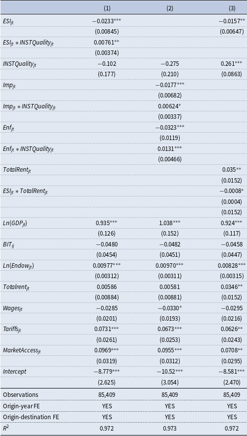
In column (1) of Table 3, we decompose the ESI into its two components: implementation and enforcement. The resultsFootnote 9 show that only the implementation component is statistically significant and negatively associated with FDI, suggesting that foreign investors respond primarily to formal policy commitments, such as the adoption of climate legislation and international agreements. These measures send clear and credible signals of future regulatory tightening, which investors may perceive as increasing long-term compliance costs. In contrast, the enforcement component, measured by the ratio of predicted to actual emissions intensity following Brunel and Levinson (Reference Brunel and Levinson2013), is not statistically significant. Although the average enforcement score exceeds one (1.08), this measure reflects aggregate outcomes rather than observable enforcement mechanisms like inspections or penalties. As such, enforcement may be less transparent or consistent, especially in countries with weaker institutional frameworks. This makes it more difficult for foreign investors to assess its reliability or impact when making location decisions. By contrast, the formal adoption of environmental laws and international agreements provides a clearer signal of future regulatory burdens. These results align with a forward-looking interpretation of the PHH, whereby firms adjust their investment strategies based on anticipated compliance costs associated with policy implementation, rather than the current effectiveness of enforcement.
Table 3. Decomposition of the ESI and non-linearity

Robust standard errors clustered at the country-pair level in parentheses.
***
p $\lt$
0.01, **
p
$\lt$
0.01, **
p $\lt$
0.05, *
p
$\lt$
0.05, *
p $\lt$
0.1.
$\lt$
0.1.
In column (2), where we further break down the implementation component into national and international policies, we find that it is specifically domestic environmental regulations, rather than international agreements, that foreign investors perceive as restrictive. This aligns with the distinction between bottom-up and top-down policies (Green et al. Reference Green, Sterner and Wagner2014). Bottom-up policies, often implemented at the national or sub-national level, are better tailored to local conditions and allow for decentralized experimentation. In contrast, top-down international agreements face challenges such as differing levels of ambition, regulatory incompatibilities, and weak enforcement, which limit their credibility. Thus, foreign investors respond more strongly to national regulations that concretely affect their operations. While not directly influential, international frameworks can play a supportive role by enhancing their credibility and encouraging more ambitious national action.
Non linearity
To explore the relationship between environmental regulation and FDI in more detail, we create a dummy variable for each quintile of the distribution of host countries’ ESI. We then interact these dummy variables with the ESI of the host country. This method allows us to explore potential non-linearities in the relationship between environmental regulation and FDI. Column (3) of table 3 summarizes our results. We find that the relationship between environmental regulation and FDI appears to be non-linear. Indeed, the coefficients associated with the first and second quintiles of the distribution of host countries’ ESI are not statistically significant at the 5% level, while the coefficients for the upper quintiles are significant and negative. Moreover, the coefficient associated with the third quintile is statistically higher than that of the last quintile of the distribution.Footnote 10 This non-linear relationship suggests that it is only after a certain threshold of environmental regulation has been reached that overly stringent regulations may impose additional costs or operational constraints that discourage foreign investors.
5.2 Heterogeneity among countries
Host country heterogeneity
In this Section we examine the heterogeneity of the results with respect to the level of development of the host country. To do this, we introduce interaction terms between the ESI and dummies capturing the level of development of the host country, namely high-income $HI$
(GNI per capita above
$HI$
(GNI per capita above $\$13,846$
), upper-middle income
$\$13,846$
), upper-middle income $UMI$
(GNI per capita between
$UMI$
(GNI per capita between $\$4,466$
and
$\$4,466$
and $\$13,845$
), lower-middle income
$\$13,845$
), lower-middle income $LMI$
(GNI per capita between
$LMI$
(GNI per capita between $\$1,136$
and
$\$1,136$
and $\$4,465$
) and low-income
$\$4,465$
) and low-income $LI$
(GNI per capita below
$LI$
(GNI per capita below $\$1,135$
).Footnote
11
Table 4 shows the results for all types of countries of origin.Footnote
12
$\$1,135$
).Footnote
11
Table 4 shows the results for all types of countries of origin.Footnote
12
Table 4. Host country heterogeneity in income

Robust standard errors clustered at the country-pair level in parentheses.
***
p $\lt$
0.01, **
p
$\lt$
0.01, **
p $\lt$
0.05, *
p
$\lt$
0.05, *
p $\lt$
0.1.
$\lt$
0.1.
The results are qualitatively similar to those in Table D1, indicating that stricter environmental regulations are associated with a decrease in inward FDI, regardless of a country’s level of development. However, different patterns emerge when looking at groups of countries. For FDI located in high-income countries, the overall negative effect of ESI is slightly milder ( $-0.0155$
) compared to the average. This may be related to their advanced regulatory frameworks and robust institutions, which may mitigate the negative impact of strict environmental regulations on FDI. Conversely, for emerging and developing countries, the negative impact is significantly higher than for developed countries. As these countries are often known as pollution havens, the increasing regulatory framework plays a stronger role in the location of FDI. This may also be because these countries often lack the infrastructure and institutional capacity to effectively implement and enforce environmental regulations, making them more burdensome for foreign investors.
$-0.0155$
) compared to the average. This may be related to their advanced regulatory frameworks and robust institutions, which may mitigate the negative impact of strict environmental regulations on FDI. Conversely, for emerging and developing countries, the negative impact is significantly higher than for developed countries. As these countries are often known as pollution havens, the increasing regulatory framework plays a stronger role in the location of FDI. This may also be because these countries often lack the infrastructure and institutional capacity to effectively implement and enforce environmental regulations, making them more burdensome for foreign investors.
These results confirm the heterogeneous nature of the “pollution haven hypothesis.” In particular, they suggest that environmental regulations have a more pronounced impact on FDI to less developed and emerging economies. This observation supports the notion that firms from developed countries have increasingly outsourced production to emerging economies such as China to take advantage of lower production costs and less stringent environmental regulations. However, we observe from columns (4) that the PHH does not hold for bilateral FDI sourced from from low-middle and low-income economies. This phenomenon may be due to the nuanced interplay of factors influencing investment decisions across income groups. Factors beyond environmental regulations, such as market access, institutional quality and labor costs, may play a crucial role in shaping FDI flows.
Institutional quality
The presence of corruption in a country may affect the relationship between environmental stringency and FDI. To investigate this, we introduce interaction terms between the ESI and the control of corruption indicator and report the results in Table 5.Footnote 13
Table 5. Institution quality, resource rent and environmental regulation
Robust standard errors clustered at the country-pair level in parentheses.
***
p $\lt$
0.01, **
p
$\lt$
0.01, **
p $\lt$
0.05, *
p
$\lt$
0.05, *
p $\lt$
0.1.
$\lt$
0.1.
In column (1), our results indicate that better governance mitigates the negative impact of strict environmental policies on FDI inflows. Specifically, a one-unit increase in the institutional quality index tends to reduce the negative effect of ESI on FDI by about 0.7%. This suggests that in countries with low corruption, stringent environmental policies are perceived as less burdensome for investment strategies. While the overall effect of stringent environmental policies remains negative, the mitigation provided by higher institutional quality means that investors view these policies as more predictable and less likely to be undermined by inconsistent enforcement. In corrupt environments, even if strong environmental policies are in place, their enforcement may be inconsistent. This brings us to the decomposition of our indicator to see whether corruption primarily affects the implementation (policy announcements) or the enforcement (actual abatement efforts) of environmental regulations. As expected, in column (2) we find that corruption mainly affects the enforcement aspect of the indicator. Bribes and corrupt practices may allow companies to circumvent regulations, leading to environmental degradation and reduced investor confidence.
Natural resource seekers
Another aspect we want to consider is if host countries dependent on natural resource rents experience unique dynamics in the relationship between environmental regulation and inward FDI. Countries with abundant natural resources, especially those involved in extractive industries, often face significant environmental challenges due to their economic activities.
In column (3) of Table 5, we introduce interaction terms between the ESI and total natural resource rents. Our results indicate that the more a country relies on natural resource rents, the more pronounced the deterrent effect of environmental stringency on inward FDI. This suggests that in economies where polluting activities, such as extractive industries, predominate, stringent environmental regulations act as a stronger deterrent to foreign investment.
Table 6. Impact of ESI distance

Robust standard errors clustered at the country-pair level in parentheses.
***
p $\lt$
0.01, **
p
$\lt$
0.01, **
p $\lt$
0.05, *
p
$\lt$
0.05, *
p $\lt$
0.1.
$\lt$
0.1.
Source country and ESI distance
Building on previous research on institutional distance (Aleksynska and Havrylchyk, Reference Aleksynska and Havrylchyk2013), we propose the concept of “environmental stringency distance,” constructed as the absolute difference between the ESI of home and host countries. Our aim is to investigate whether investor reactions extend beyond the environmental policy stringency of the host country to include differences in the level of environmental policy stringency. We then estimate the gravity equation described in Eq. (6), including year of origin, origin-destination, destination and year fixed effects. Table 6 shows interesting results.Footnote 14 Column (1) and (3) shows that the absolute difference has no effect on FDI, suggesting that countries with highly heterogeneous environmental policies are not necessarily attracted. However, to gain a deeper insight into this issue, in columns (2) and (4) of Table 6 we decompose the absolute distance in environmental policy stringency into positive and negative ESI distances. A positive ESI distance denotes a scenario where the ESI of the source country exceeds that of the host country, indicating a preference among investors for lower levels of environmental policy. Conversely, a negative ESI distance arises when the ESI of the source country is lower than that of the host country, implying a preference for a higher level of environmental policy. This disaggregation is driven by the hypothesis that the effects of positive and negative ESI distances are not symmetric; investing in countries with much stricter environmental policies may be particularly attractive. The regression results show the importance of this disaggregation for investors. Specifically, we observe that investors are attracted to countries with less stringent environmental policies when investing in jurisdictions with lower levels of stringency. Moreover, when investors direct their investments to countries with stricter environmental policies than their home country, they still show a preference for countries with less stringent environmental regulations. Consistently, the effect size is slightly larger when investors allocate capital to countries with stricter environmental policies.
Looking at the other components of the model, five appear to be statistically significant. The sum of GDP and differences in GDP together suggest that while a larger combined economic size is attractive due to its market potential, significant differences in economic development levels (as indicated by GDP per capita) may be a deterrent, especially regarding horizontal FDI (Brainard, Reference Brainard1997). For differences in the capital-labor ratio, the positive significance suggests that investors are motivated to exploit different endowments to optimize production costs and efficiency. This is in line with economic theory on vertical FDI (Helpman, Reference Helpman1984), where countries with different capital-labor compositions may offer comparative advantages. Finally, the wage differential is particularly noteworthy. The positive significance indicates that larger differences in wage regulations and minimum wages attract FDI. This reflects the strategic importance of labor market conditions in investment decisions, where firms seek to minimize operating costs in order to maximize returns.
6. Robustness tests
To further strengthen the robustness of our results, we conduct a series of alternative tests using different methodologies.
ESI and EPS
In columns (1) and (2) of Table D4, we compare the estimation results using the EPS as an alternative to the ESI to measure environmental stringency. This index, described in Section 3.3, is widely used in the empirical literature. As with Table D1, we report standardized coefficients in Appendix Table D5 to ensure comparability across specifications. We therefore estimate the augmented structural gravity model using both indicators on the same sample of countries. Column (1) presents the results for the ESI, while column (2) presents the results for the EPS. The results are quantitatively and qualitatively similar in both regressions, confirming the reliability of our new indicator as a measure of environmental stringency.
Alternative measures of enforcement
In column (3), we address the enforcement aspect of environmental policies using a different measurement approach. Specifically, we apply the EPI scoring methodology to recalculate the climate change mitigation category using the weights assigned in the 2022 Technical Annex. Key variables in this analysis include the growth rate of $CO_2$
, projected GHG emissions in 2050, and the growth rate of F-gases. As with the previous indicators, we standardize this enforcement index to ensure comparability (see Appendix Table D5). The results of this alternative method, reported in column (3), are consistent with our previous findings (see column (1) of Table 3), further confirming the insignificance of government enforcement efforts. In column (4), we refine our enforcement index by calculating average emissions per sector for different groups of countries, taking into account regional differences in emission intensity. This adjustment confirms the robustness of our results, as no significant changes in the results are observed.
$CO_2$
, projected GHG emissions in 2050, and the growth rate of F-gases. As with the previous indicators, we standardize this enforcement index to ensure comparability (see Appendix Table D5). The results of this alternative method, reported in column (3), are consistent with our previous findings (see column (1) of Table 3), further confirming the insignificance of government enforcement efforts. In column (4), we refine our enforcement index by calculating average emissions per sector for different groups of countries, taking into account regional differences in emission intensity. This adjustment confirms the robustness of our results, as no significant changes in the results are observed.
Leads and lags
We also test the robustness of our results to the inclusion of leads and lags on the ESI variable in the structural gravity equations. We add two leads and two lags and estimate the structural gravity model as an event study design. Figure D1 shows the estimation results. We find no significant impact of the two leads of the ESI variable on FDI, suggesting no anticipatory effects of environmental policies for FDI. Furthermore, the two lags are significant and negative, confirming our previous results and revealing a persistent effect of environmental policies on FDI.
7. Conclusion
This paper examines the relationship between environmental regulation and FDI using a comprehensive bilateral dataset covering 111 source and 121 host countries from 2001 to 2018. A key contribution is the development of a novel ESI that distinguishes between two dimensions of environmental policy: implementation—capturing formal regulatory commitment—and enforcement—measured as deviations between predicted and actual emissions.
Our empirical findings, based on structural gravity models estimated using the PPML estimator, provide robust evidence of a Pollution Haven Effect. Stricter environmental regulations in host countries are associated with lower inward FDI, particularly from developed source countries.
We also document heterogeneity across country pairs. The negative impact of environmental regulation is stronger for FDI flowing into emerging economies and in contexts with higher corruption. In contrast, there is limited evidence of regulatory arbitrage in FDI flows from emerging to developed economies, reflecting differences in institutional capacity and regulatory expectations.
These results highlight the importance of regulatory design in shaping global investment patterns. While other factors—such as labor costs, governance, and resource endowments—also influence location decisions, our findings underscore the significant and differentiated role played by environmental regulation. From a policy perspective, it suggests that well-defined and credible national environmental regulations are crucial in influencing firms’ location decisions and preventing environmentally harmful relocations. Such policies generally have a more significant impact on foreign investors compared to those that are ambiguously enforced. Additionally, aligning national regulations with international environmental frameworks can enhance coordination, help to minimize regulatory arbitrage and strengthen long-term climate commitments. Furthermore, the non-linear effects observed in the data highlight the need for precise policy calibration: only countries with sufficiently stringent environmental standards experience a notable deterrent effect on FDI.
Future research could extend this work by incorporating firm-level data to account for heterogeneity in pollution intensity and compliance behavior across firms. This would allow for a more detailed examination of how environmental regulation influences investment decisions, depending on firms’ environmental characteristics and sectoral exposure.
Appendix
Appendix A: Descriptive statistics on the ESI
Table A1. Summary statistics


Figure A1. ESI by country for 2001.

Figure A2. Evolution of ESI by country group between 2000 and 2020.

Figure A3. Decomposition of the ESI for 2018.

Figure A4. ESI versus EPS coverage for 2018.
Appendix B: Descriptive statistics on bilateral FDI
Figure B1 depicts bilateral FDI stocks by country group. The left graph illustrates bilateral FDI stocks between high-income countries and the rest of the world. The right graph focuses on FDI stocks from high-income countries to lower-income groups, decomposed into upper-middle-income ( $Hi-UMi$
), lower-middle-income (
$Hi-UMi$
), lower-middle-income ( $Hi-LMi$
), and low-income (
$Hi-LMi$
), and low-income ( $Hi-Li$
) countries. The data highlight the growing concentration of FDI among high-income countries and increasing investment flows from high-income to upper-middle-income countries, underscoring the evolving patterns of global economic integration and investment strategies, respectively.
$Hi-Li$
) countries. The data highlight the growing concentration of FDI among high-income countries and increasing investment flows from high-income to upper-middle-income countries, underscoring the evolving patterns of global economic integration and investment strategies, respectively.

Figure B1. Bilateral FDI stocks over time.
Figure B2 provides a focused look at the top 10 exporters and receivers of bilateral FDI stocks for 2018. The United States stands out prominently as both the largest exporter and receiver of FDI, with bilateral FDI stocks exceeding 5,000 billion U.S. dollars in both directions. This highlights the central role of the U.S. in global investment flows, reflecting its economic size and the attractiveness of its market. Other significant exporters include the Netherlands, the United Kingdom, and Luxembourg. On the receiving end, besides the U.S., the Netherlands and Luxembourg also feature prominently, indicating their attractiveness as investment destinations. Germany, the United Kingdom, Switzerland, and other countries such as Ireland, France, Japan, and Spain are also key receivers, showcasing their strong economic foundations and stability which attract foreign investments.
Figure B3 presents the distribution of global inward FDI by sector in 2018, while Figure B4 shows the corresponding sectoral emission intensities.Footnote 15 These figures rely on detailed sectoral FDI data from the World Bank for the final year of our study period (Steenbergen et al. Reference Steenbergen, Liu, Latorre and Zhu2022). However, since this sectoral database is only available from 2008 onward, thereby excluding the pre-Kyoto Protocol period, we chose not to rely on it for the main analysis. Nonetheless, the sectoral database remains valuable to show the distribution of FDI across industries and the share of polluting sectors, ensuring that our results are not driven by an excessive concentration of FDI in these specific sectors. A high correlation (85.75%) between the sectorally aggregated data and our primary aggregate dataset supports their comparability. This alignment stems from the fact that both datasets are built upon the same underlying source, namely UNCTAD, the IMF CDIS dataset, and the OECD bilateral FDI statistics.
Moving to the data, we find that inward FDI is mainly concentrated in a non-pollution-intensive sector, namely Financial and insurance activities (44.2%). Traditionally dirty sectors like Mining and quarrying and Electricity and gas account for a relatively small share of total FDI (4.0 and 1.3%, respectively). Meanwhile, the Manufacturing sector represents approximately 22% of total inward FDI and encompasses a mix of low and high-emission industries.Footnote
16
Among these, the petroleum, chemical, pharmaceutical, rubber and plastic industry stands out as both highly polluting and significantly represented in the FDI stock ( $6.97\%$
). This suggests that foreign investments are not exclusively driven by pollution-intensive sectors, and that the sectoral composition of FDI reflects a balanced mix. As such, the use of aggregate FDI measures neither overstate nor understate the pollution haven effect, capturing its environmental impact without being dominated by the cleanest or dirtiest sectors.
$6.97\%$
). This suggests that foreign investments are not exclusively driven by pollution-intensive sectors, and that the sectoral composition of FDI reflects a balanced mix. As such, the use of aggregate FDI measures neither overstate nor understate the pollution haven effect, capturing its environmental impact without being dominated by the cleanest or dirtiest sectors.

Figure B2. Main source and host of FDI in 2018.

Figure B3. Sectoral composition of FDI.

Figure B4. Emission intensities by sector.
Appendix C: Countries and variables in the empirical analysis
Table C1. List of countries

Table C2. Variable definitions and sources

Table C3. Descriptive statistics

Appendix D: Non-standardized coefficients and robustness checks
Table D1. Baseline results

Robust standard errors clustered at the country-pair level in parentheses in columns (1) to (8). Bootstrapped standard errors (1000 replications) in parentheses for column (9).
***
p $\lt$
0.01, **
p
$\lt$
0.01, **
p $\lt$
0.05, *
p
$\lt$
0.05, *
p $\lt$
0.1.
$\lt$
0.1.
Table D2. Results of the first-stage regression

Robust standard errors clustered at the country-pair level in parentheses.
***
p $\lt$
0.01, **
p
$\lt$
0.01, **
p $\lt$
0.05, *
p
$\lt$
0.05, *
p $\lt$
0.1.
$\lt$
0.1.
Table D3. Results of the regression on the instrument

Robust standard errors clustered at the country-pair level in parentheses.
***
p $\lt$
0.01, **
p
$\lt$
0.01, **
p $\lt$
0.05, *
p
$\lt$
0.05, *
p $\lt$
0.1.
$\lt$
0.1.
Table D4. Robustness checks with non-standardized coefficients

Robust standard errors clustered at the country-pair level in parentheses.
***
p $\lt$
0.01, **
p
$\lt$
0.01, **
p $\lt$
0.05, *
p
$\lt$
0.05, *
p $\lt$
0.1.
$\lt$
0.1.
Table D5. Robustness checks with standardized coefficients

Robust standard errors clustered at the country-pair level in parentheses.
***
p $\lt$
0.01, **
p
$\lt$
0.01, **
p $\lt$
0.05, *
p
$\lt$
0.05, *
p $\lt$
0.1.
$\lt$
0.1.

Figure D1. Leads and lags of ESI.
The figure depicts estimated coefficient from the estimation of the structural gravity including two leads and two lags of the variable ESI. Regressions include all control variables and well as country-pair and origin country-year fixed effects.


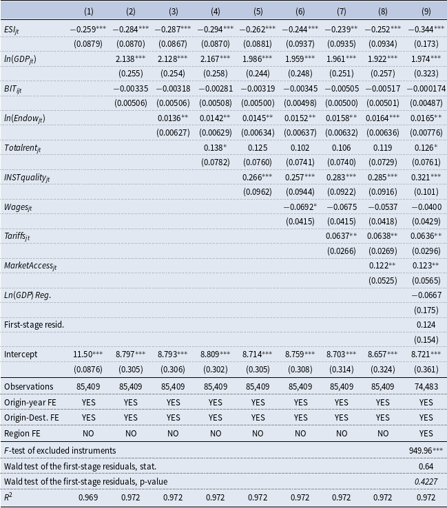
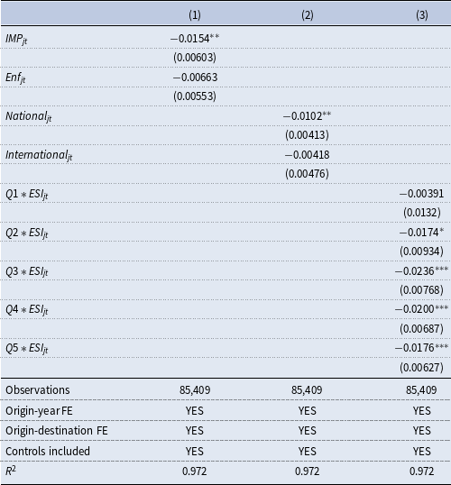


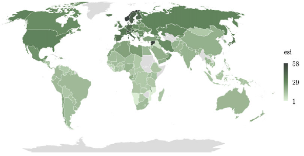


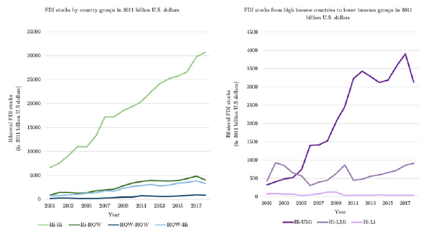


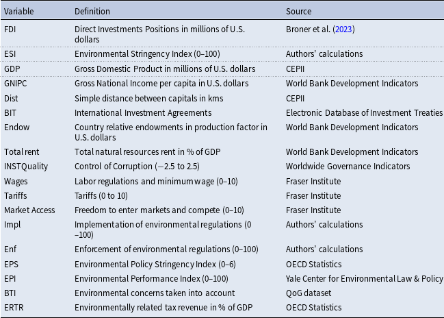


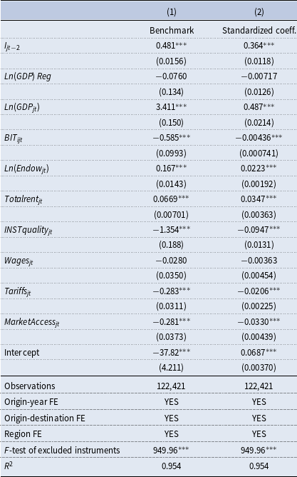


 Open access