2.2.1 Abundance changes due to FDU

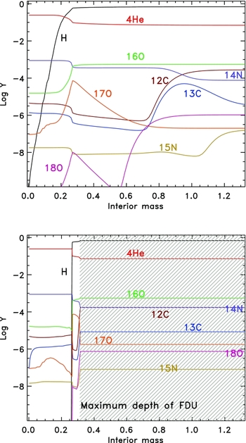
The material mixed to the envelope by the FDU has been subjected to partial H burning, which means it is still mostly H but with some added ⁴He and the products of CN cycling. Figure 5 shows the situation for a 2 M_⊙ model. The upper panel shows the abundance profile after the star has departed the main sequence and prior to the FDU. We have plotted the major species and some selected species involved in the CNO cycles. The lower panel is taken at the time of the maximum depth of the convective envelope. The timescale for convective mixing is much shorter than the evolution timescale so mixing essentially homogenises the region instantly, as far as we are concerned.

Figure 5.

Composition profiles from the 2 M_⊙, Z = 0.02 model. The top panel illustrates the interior composition after the main sequence and before the FDU takes place, showing mostly CNO isotopes. The lower panel shows the composition at the deepest extent of the FDU (0.31 M_⊙), where the shaded region is the convective envelope. Surface abundance changes after the FDU include: a reduction in the C/O ratio from 0.50 to 0.33, in the ¹²C/¹³C ratio from 86.5 to 20.5, an increase in the isotopic ratio of ¹⁴N/¹⁵N from 472 to 2 188, a decrease in ¹⁶O/¹⁷O from 2 765 to 266, and an increase in ¹⁶O/¹⁸O from 524 to 740. Elemental abundances also change: [C/Fe] decreases by about 0.20, [N/Fe] increases by about 0.4, and [Na/Fe] increases by about 0.1. The helium abundance increases by ΔY ≈ 0.012.

Typical surface abundance changes from FDU are an increase in the ⁴He abundance by ΔY ≈ 0.03 (in mass fraction), a decrease in the ¹²C abundance by about 30%, and an increase in the ¹⁴N and ¹³C abundances. In Table 1 we provide the predicted post-FDU and SDU values for model stars with masses between 1 and 8 M_⊙ at Z = 0.02. We include the He mass fraction, Y, the isotopic ratios of C, N, and O, and the mass fraction of Na.

Table 1.

Predicted post-FDU and SDU values for model stars with masses between 1 and 8 M_⊙ at Z = 0.02. We include the helium mass fraction, Y, the isotopic ratios of carbon, nitrogen, and oxygen, and the mass fraction of sodium. Initial values are given in the first row.

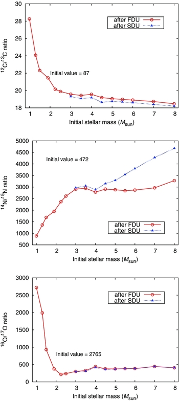
The C isotopic ratio is a very useful tracer of stellar evolution and nucleosynthesis in low- and intermediate-mass stars. First, this is because the ¹²C/¹³C ratio is one of the few isotopic ratios that can be readily derived from stellar spectra which means that there are large samples of stars for comparison to theoretical calculations (e.g., Gilroy & Brown Reference Gilroy and Brown1991; Gratton et al. Reference Gratton, Sneden, Carretta and Bragaglia2000; Smiljanic et al. Reference Smiljanic, Gauderon, North, Barbuy, Charbonnel and Mowlavi2009; Mikolaitis et al. Reference Mikolaitis, Tautvaišienė, Gratton, Bragaglia and Carretta2010; Tautvaišienė et al. Reference Tautvaišienė, Barisevičius, Chorniy, Ilyin and Puzeras2013). Second, the C isotope ratio is predicted to vary significantly at the surface as a result of the FDU (and SDU) as shown in Figure 6 and in Table 1. This figure shows that the number ratio of ¹²C/¹³C drops from its initial value (typically about 89 for the Sun) to lie between 18 and 26 (see also Charbonnel Reference Charbonnel1994; Boothroyd & Sackmann Reference Boothroyd and Sackmann1999). Comparisons for intermediate-mass stars are in relatively good agreement with the observations, to within ~ 25% (El Eid Reference El Eid1994; Charbonnel Reference Charbonnel1994; Boothroyd & Sackmann Reference Boothroyd and Sackmann1999; Santrich, Pereira, & Drake Reference Santrich, Pereira and Drake2013). But the agreement found at low luminosities is not seen further up the RGB (e.g., Charbonnel Reference Charbonnel1995), as discussed in Section 2.2.4.

Figure 6.

Surface abundance predictions from Z = 0.02 models showing the ratio (by number) of ¹²C/¹³C, ¹⁴N/¹⁵N, and ¹⁶O/¹⁷O after the first dredge-up (red solid line) and second dredge-up (blue dotted line).

In Figure 7 we show the innermost mass layer reached by the convective envelope during FDU (solid lines) and SDU (dashed lines) as a function of the initial stellar mass and metallicity. The deepest FDU occurs in the Z = 0.02 models at approximately 2.5 M_⊙ with a strong metallicity dependence for models with masses over about 3 M_⊙ (Boothroyd & Sackmann Reference Boothroyd and Sackmann1999). In contrast there is little difference in the depth of the second dredge-up for models with ≳ 3.5 M_⊙ regardless of metallicity. In even lower metallicity intermediate-mass stars, the RGB phase is skipped altogether because core He burning is ignited before the model star reaches the RGB so that the first change to the surface composition is actually due to the second dredge-up.

Figure 7.

Innermost mass layer reached by the convective envelope during the first dredge-up (solid lines) and second dredge-up (dashed lines) as a function of the initial stellar mass and metallicity. The mass co-ordinate on the y-axis is given as a fraction of the total stellar mass (M _du/M ₀)—from Karakas (Reference Karakas2003).

One check on the models concerns the predictions for O isotopes. Broadly, the CNO cycles produce ¹⁷O but significantly destroy ¹⁸O, with the result that the FDU should increase the observed ratio of ¹⁷O/¹⁶O and decrease the observed ratio of ¹⁸O/¹⁶O (e.g., Table 1 and Dearborn Reference Dearborn1992). Spectroscopic data, where available, seem to agree reasonably well with the FDU predictions (Dearborn Reference Dearborn1992; Boothroyd, Sackmann, & Wasserburg Reference Boothroyd, Sackmann and Wasserburg1994), but see also Section 2.2.4.

The effect of the first dredge-up on other elements (besides lithium, which we discuss in Section 2.4 below) is relatively minor. It is worth noting that there is some dispute about the status of sodium. Figure 8 shows that sodium is not predicted to be significantly enhanced in low-mass stars by the FDU or by extra-mixing processes (Charbonnel & Lagarde Reference Charbonnel and Lagarde2010) at disk metallicities. This agrees with El Eid & Champagne (Reference El Eid and Champagne1995) who find modest enhancements in low mass (0.1 dex) and intermediate mass (0.2 – 0.3 dex) stars. Observations are in general agreement with models with masses ≳ 2 M_⊙, where enhancements of up to [Na/Fe] ≲ 0.3 are found in stars up to 8 M_⊙ at Z = 0.02 (Figure 8). This result is confirmed by observations that show only mild enhancements of [Na/Fe] ≲ +0.2 (Hamdani et al. Reference Hamdani, North, Mowlavi, Raboud and Mermilliod2000; Smiljanic et al. Reference Smiljanic, Gauderon, North, Barbuy, Charbonnel and Mowlavi2009). But this is in contradiction with other studies showing typical overabundances of + 0.5 (Bragaglia et al. Reference Bragaglia2001; Jacobson, Friel, & Pilachowski Reference Jacobson, Friel and Pilachowski2007; Schuler, King, & The Reference Schuler, King and The2009). The reasons for the conflicting results are not well understood; we refer to Smiljanic (Reference Smiljanic2012) for a detailed discussion of observational uncertainties.

Figure 8.

Predicted [Na/Fe] after the FDU and SDU for the Z = 0.02 models.

2.2.2 The onset of FDU

Theoretical models must confront observations for us to verify that they are reliable or identify where they need improvements. In the current context there are two related comparisons to be made: the expected nucleosynthesis, which we addressed above, and the structural aspects. In this section we look at the predictions for the location of the start of FDU and in the next section we compare the observed location of the bump in the luminosity function to theoretical models.

During the evolution up the giant branch there are three significant points, as illustrated in Figure 3:

• • the luminosity at which the surface abundances start to change;

• • the maximum depth of the FDU;

• • the luminosity of the bump.

Note that these are not independent—the maximum depth of the FDU determines where the abundance discontinuity occurs, and that determines the position of the bump. Similarly, the resulting compositions are dependent on the depth of the FDU and we are not free to adjust that without consequences for both the observed abundances and the location of the bump.

The obvious question is how closely do these points match the observations? Perhaps the best place to look is in star clusters, as usual. Gilroy & Brown (Reference Gilroy and Brown1991) found that the ratios of C/N and ¹²C/¹³C at the onset of the FDU matched the models quite well, as reported in Charbonnel (Reference Charbonnel1994). Mishenina et al. (Reference Mishenina, Bienaymé, Gorbaneva, Charbonnel, Soubiran, Korotin and Kovtyukh2006) also looked at C/N and various other species, and the data again seem to match models for the onset of the FDU. Of course the onset is very rapid and the data are sparse. This is also seen in the study by Chanamé, Pinsonneault, & Terndrup (Reference Chanamé, Pinsonneault and Terndrup2005) who found that the C isotopic ratio in M67 fitted the models rather well (see their Figures 13 and 14). For field giants (with − 2 < [Fe/H] < −1) the data are not so good, with mostly lower limits for ¹²C/¹³C making it hard to identify the exact onset of the FDU (see Chanamé et al. Reference Chanamé, Pinsonneault and Terndrup2005, Figure 16). Better data over a larger range in luminosity in many clusters are needed to check that the models are not diverging from reality at this early stage in the evolution.

2.2.3 The bump in the luminosity function

We now move to an analysis of the luminosity function (LF) bump. There is much more literature here, dating back to Sweigart (Reference Sweigart, Philip and Hayes1978) where it was shown that the bump reduced in size and appeared at higher luminosities as either the He content increased or the metallicity decreased. Indeed, at low metallicity (say [Fe/H] ≲ −1.6) it can be hard to identify the LF bump, and Fusi Pecci et al. (Reference Pecci, Ferraro, Crocker, Rood and Buonanno1990) combined data for the GCs M92, M15, and NGC 5466 so that they could reliably identify the bump in these clusters (all of similar metallicity). Their conclusion, based on a study of 11 clusters, was that the theoretical position of the bump was 0.4 mag too bright.

The next part of the long history of this topic was the study by Cassisi & Salaris (Reference Cassisi and Salaris1997) with newer models who concluded that there was no discrepancy within the theoretical uncertainty. Idealised models show a discontinuity in composition at the mass where the convective envelope reached its maximum inward extent. But in reality this discontinuity is likely to be a steep profile, with a gradient determined by many things, such as the details of mixing at the bottom of the convective envelope. It is likely that gravity waves and the possibility of partial overshoot would smooth this profile through entrainment, and Cassisi, Salaris, & Bono (Reference Cassisi, Salaris and Bono2002) showed that such uncertainties do cause a small shift in the position of the bump but they are unlikely to be significant.

Riello et al. (Reference Riello2003) looked at 54 Galactic GCs and found good agreement between theory and observation, both for the position of the bump itself as well as the number of stars (i.e., evolutionary timescales) in the bump region. The only caveat was that for low metallicities there seemed to be a discrepancy but it was hard to quantify due to the low number of stars available. A Monte Carlo study by Bjork & Chaboyer (Reference Bjork and Chaboyer2006) concluded that the difference between theory and observation was no larger than the uncertainties in both of those quantities. In what seems to be emerging as a consensus, Di Cecco et al. (Reference Di Cecco2010) found that the metal-poor clusters showed a discrepancy of about 0.4 mag, and that variations in CNO and α-elements (e.g., O, Mg, Si, Ti) did not improve the situation. These authors did point out that the position of the bump is sensitive to the He content and since we now believe that there are multiple populations in most GCs, this is going to cause a spread in the position of the LF bump.

It would appear that a reasonable conclusion is that the theoretical models are in good agreement, while perhaps being about 0.2 mag too bright (Cassisi et al. Reference Cassisi, Marín-Franch, Salaris, Aparicio, Monelli and Pietrinferni2011), except for the metal-poor regime where the discrepancy may be doubled to 0.4 mag, although this is plagued by the bump being small and harder to observe. Nataf et al. (Reference Nataf, Gould, Pinsonneault and Udalski2013) find evidence for a second parameter, other than metallicity, being involved. In their study of 72 globular clusters there were some that did not fit the models well, and this was almost certainly due to the presence of multiple populations. This reminds us again that quantitative studies must include these different populations and that this could be the source of some of the discrepancies found in the literature.

The obvious way to decrease the luminosity of the bump is to include some overshooting inward from the bottom of the convective envelope. This will push the envelope deeper and will shift the LF bump to lower luminosities. Of course this deeper mixing alters the predictions of the FDU; however it appears that there is a saturation of composition changes such that the small increase needed in the depth of the FDU does not produce an observable difference in the envelope abundances (Kamath et al. Reference Kamath, Karakas and Wood2012; Angelou 2013, private communication).

2.2.4 The need for extra-mixing

We have seen that the predictions for FDU are largely in agreement with the observations. However when we look at higher luminosities we find that something has changed the abundances beyond the values predicted from FDU. Standard models do not predict any further changes on the RGB once FDU is complete. Something must be occurring in real stars that is not predicted by the models.

For low-mass stars the predicted trend of the post-FDU ¹²C/¹³C ratio is a rapid decrease with increasing initial mass as illustrated in Figure 6. Yet this does not agree with the observed trend. For example, observations of the ¹²C/¹³C ratio in open metal-rich clusters reveal values of ≲ 20, sometimes ≲ 10 (e.g., Gilroy Reference Gilroy1989; Smiljanic et al. Reference Smiljanic, Gauderon, North, Barbuy, Charbonnel and Mowlavi2009; Mikolaitis et al. Reference Mikolaitis, Tautvaišienė, Gratton, Bragaglia and Carretta2010) well below the predicted values of ≈ 25 − 30. The deviation between theory and observation is even more striking in metal-poor field stars and in giants in GCs (e.g., Pilachowski et al. Reference Pilachowski, Sneden, Kraft and Langer1996; Gratton et al. Reference Gratton, Sneden, Carretta and Bragaglia2000, Reference Gratton, Sneden and Carretta2004; Cohen, Briley, & Stetson Reference Cohen, Briley and Stetson2005; Origlia, Valenti, & Rich Reference Origlia, Valenti and Rich2008; Valenti, Origlia, & Rich Reference Valenti, Origlia and Rich2011).

The observed trend is in the same direction as the FDU: i.e., as if we are mixing in more material that has been processed by CN cycling, so that ¹²C decreases just as ¹³C and ¹⁴N increase. Indeed, in some GCs we see a clear decrease in [C/Fe] with increasing luminosity on the RGB (see Angelou et al. Reference Angelou, Church, Stancliffe, Lattanzio and Smith2011, Reference Angelou, Stancliffe, Church, Lattanzio and Smith2012, and references therein). If some form of mixing can connect the hot region at the top of the H-burning shell with the convective envelope then the results of the burning can be seen at the surface. These observations have been interpreted as evidence for extra mixing taking place between the base of the convective envelope and the H shell.

Further evidence comes from observations of the fragile element Li (Pilachowski, Sneden, & Booth Reference Pilachowski, Sneden and Booth1993; Lind et al. Reference Lind, Primas, Charbonnel, Grundahl and Asplund2009) which essentially drops at the FDU to the predicted value of A(Li) ≈ 1Footnote ³ , but for higher luminosities decreases to much lower abundances of A(Li) ≈ 0 to − 1. Again, this can be explained by exposing the envelope material to higher temperatures, where Li is destroyed. So just as for the C isotopes the observations argue for some form of extra mixing to join the envelope to the region of the H-burning shell (see also Section 2.4).

We discussed O isotopes earlier as a diagnostic of the FDU. Although these ratios may not be so easy to determine spectroscopically, the science of meteorite grain analysis (for reviews see Zinner Reference Zinner1998; Lodders & Amari Reference Lodders and Amari2005) offers beautiful data on O isotopic ratios from Al₂O₃ grains. We expect that these grains would be expelled from the star during periods of mass loss and would primarily sample the tip of the RGB or the AGB. Some of these data show good agreement with predictions for the FDU, while a second group clearly require further ¹⁸O destruction. This can be provided by the deep-mixing models of Wasserburg, Boothroyd, & Sackmann (Reference Boothroyd, Sackmann and Wasserburg1995) and Nollett, Busso, & Wasserburg (Reference Nollett, Busso and Wasserburg2003). Hence pre-solar grains contain further evidence for the existence of some kind of extra mixing on the RGB.

We note here that a case has been made for some similar form of mixing in AGB envelopes as we discuss later in Section 4.3.

2.2.5 The ³He problem

Another piece of evidence for deep-mixing concerns the stellar yield of ³He, as discussed recently by Lagarde et al. (Reference Lagarde, Charbonnel, Decressin and Hagelberg2011, Reference Lagarde, Romano, Charbonnel, Tosi, Chiappini and Matteucci2012). We now have good constraints on the primordial abundance of ³He, from updated Big Bang Nucleosynthesis calculations together with WMAP data. The currently accepted value is ³He/H = 1.00 ± 0.07 × 10^{− 5} according to Cyburt, Fields, & Olive (Reference Cyburt, Fields and Olive2008) and ³He/H = 1.04 ± 0.04 × 10^{− 5} according to Coc et al. (Reference Coc, Vangioni-Flam, Descouvemont, Adahchour and Angulo2004). This is within a factor of two or three of the best estimates of the local value in the present interstellar medium of ³He/H = 2.4 ± 0.7 × 10^{− 5} according to Gloeckler & Geiss (Reference Gloeckler and Geiss1996), a value also in agreement with the measurements in Galactic HII regions by Bania, Rood, & Balser (Reference Bania, Rood and Balser2002). This indicates a very slow growth of the ³He content over the Galaxy’s lifetime.

However, the evolution of low-mass stars predicts that they produce copious amounts of ³He. This isotope is produced by the pp chains and when the stars reach the giant branches their stellar winds carry the ³He into the interstellar medium. Current models for the chemical evolution of the Galaxy, using standard yields for ³He, predict that the local interstellar medium should show ³He/H ≈ 5 × 10^{− 5} (Lagarde et al. Reference Lagarde, Romano, Charbonnel, Tosi, Chiappini and Matteucci2012) which is about twice the observed value.

It has long been recognised that one way to solve this problem is to change the yield of ³He in low-mass stars to almost zero (Charbonnel Reference Charbonnel1995). In this case the build up of ³He over the lifetime of the Galaxy will be much slower. One way to decrease the yield of ³He is to destroy it in the star on the RGB while the extra mixing is taking place. We discuss this further in Section 2.3.

2.3.1 The onset of extra mixing

So where does the extra-mixing begin and what can it be? Observations generally indicate that the conflict between theory and observation does not arise until the star has reached the luminosity of the bump in the LF. This is beautifully demonstrated in the Li data from Lind et al. (Reference Lind, Primas, Charbonnel, Grundahl and Asplund2009) which we reproduce in Figure 9 together with a theoretical calculation for a model of the appropriate mass and composition for NGC 6397 (Angelou 2013, private communication). The left panel shows the measured A(Li) values for the stars as a function of magnitude. The near constant values until M_V ≈ 3.3 are perfectly consistent with the models. It is at this luminosity that the convective envelope starts to penetrate into regions that have burnt ⁷Li, diluting the surface ⁷Li content. This stops when the envelope reaches its maximum extent, near M_V ≈ 1.5. Then there is a sharp decrease in the Li abundance once the luminosity reaches M_V ≈ 0, which roughly corresponds to the point where the H shell has reached the discontinuity left behind by FDU (see right panel). This is the same position as the bump in the LF. Note that there is a small discrepancy between the models and the data, as shown in the figure and as discussed in Section 2.2.3.

Figure 9.

Observed behaviour of Li in stars in NGC 6397, from Lind et al. (Reference Lind, Primas, Charbonnel, Grundahl and Asplund2009), and as modelled by Angelou et al. (in preparation). The leftmost panel shows A(Li) = log ₁₀(Li/H) + 12 plotted against luminosity for NGC 6397. Moving to the right the next panel shows the HR diagram for the same stars. The next panel to the right shows the inner edge of the convective envelope in a model of a typical red-giant star in NGC 6397. The rightmost panel shows the resulting predictions for A(Li) using thermohaline mixing and C = 120 (see Section 2.3.4). Grey lines identify the positions on the RGB where the major mixing events take place. Dotted red lines identify these with the theoretical predictions in the rightmost panels.

This is the common understanding—that the deep mixing begins once the advancing H shell removes the abundance discontinuity left behind by the FDU. The reason for this is that one expects that gradients in the composition can inhibit mixing (Kippenhahn & Weigert Reference Kippenhahn and Weigert1990) and once they are removed by burning then the mixing is free to develop. It was Mestel (Reference Mestel1953) who first proposed that for a large enough molecular weight gradient one could effectively have a barrier to mixing (see also Chanamé et al. Reference Chanamé, Pinsonneault and Terndrup2005). This simple theory, combined with the very close alignment of the beginning of the extra mixing and the LF bump, has led to the two being thought synonymous. However we do note that there are discrepancies with this idea. For example it has been pointed out by many authors that there is a serious problem with the metal-poor GC M92 (Chanamé et al. Reference Chanamé, Pinsonneault and Terndrup2005; Angelou et al. Reference Angelou, Stancliffe, Church, Lattanzio and Smith2012). Here the data show a clear decrease in [C/Fe] with increasing luminosity on the RGB (Bellman et al. Reference Bellman, Briley, Smith and Claver2001; Smith & Martell Reference Smith and Martell2003), starting at M_V ≈ 1–2. The problem is that the decrease begins well before the bump in the LF, which Martell, Smith, & Briley (Reference Martell, Smith and Briley2008) place at M_V ≈ −0.5. This is a substantial disagreement. A similar disagreement was noted by Angelou et al. (Reference Angelou, Stancliffe, Church, Lattanzio and Smith2012) for M15 although possibly not for NGC 5466, despite all three clusters having a very similar [Fe/H] of ≈ − 2.

To be sure that we cannot dismiss this disagreement lightly, there is also the work by Drake et al. (Reference Drake, Ball, Eldridge, Ness and Stancliffe2011) on λ Andromeda, a mildly metal-poor ([Fe/H] ≈ −0.5) first ascent giant star that is believed to have recently completed its FDU. It is not yet bright enough for the H shell to have reached the abundance discontinuity left by the FDU, but it shows ¹²C/¹³C ≲ 20, which is below the prediction for the FDU and more in line with the value expected after extra mixing has been operating for some time. We know λ Andromeda is a binary so we cannot rule out contamination from a companion. But finding a companion that can produce the required envelope composition is not trivial. Drake et al. (Reference Drake, Ball, Eldridge, Ness and Stancliffe2011) also give the case of a similar star, 29 Draconis, thus arguing further that these exceptions are not necessarily the result of some unusual evolution. The problem demands further study because the discrepancy concerns fundamental stellar physics.

2.3.2 Rotation

It is well known that rotating stars cannot simultaneously maintain hydrostatic and thermal equilibrium, because surfaces of constant pressure (oblate spheroids) are no longer surfaces of constant temperature. Dynamical motions develop that are known as ‘meridional circulation’ and which cause mixing of chemical species. It is not our intention to provide a review of rotation in a stellar context. There are many far more qualified for such a task and we refer the reader to Heger, Langer, & Woosley (Reference Heger, Langer and Woosley2000), Tassoul (Reference Tassoul2007), Maeder & Meynet (Reference Maeder and Meynet2010), and the series of 11 papers by Tassoul and Tassoul, ending with Tassoul & Tassoul (Reference Tassoul and Tassoul1995). Note that most studies that discuss the impact of rotation on stellar evolution often ignore magnetic fields. Magnetic fields likely play an important role in the removal of angular momentum from stars as they evolve (e.g., through stellar winds; Gallet & Bouvier Reference Gallet and Bouvier2013; Mathis Reference Mathis, Goupil, Belkacem, Neiner, Lignières and Green2013; Cohen & Drake Reference Cohen and Drake2014).

Most of the literature on rotating stars concerns massive stars because they rotate faster than low- and intermediate-mass stars. Nevertheless, there is a substantial history of calculations relevant to our subject. Sweigart & Mengel (Reference Sweigart and Mengel1979) were the first to attempt to explain the observed extra mixing with meridional circulation. Later advances in the theory of rotation and chemical transport (Kawaler Reference Kawaler1988; Zahn Reference Zahn1992; Maeder & Zahn Reference Maeder and Zahn1998) led to more sophisticated models for the evolution of rotating low- and intermediate-mass stars (Palacios et al. Reference Palacios, Talon, Charbonnel and Forestini2003, Reference Palacios, Charbonnel, Talon and Siess2006).

With specific regard to the extra mixing problem on the RGB, Palacios et al. (Reference Palacios, Charbonnel, Talon and Siess2006) found that the best rotating models did not produce enough mixing to explain the decrease seen in the ¹²C/¹³C ratio on the upper RGB, above the bump in the LF. This is essentially the same result as found by Chanamé et al. (Reference Chanamé, Pinsonneault and Terndrup2005) and Charbonnel & Lagarde (Reference Charbonnel and Lagarde2010). Although one can never dismiss the possibility that a better understanding of rotation and related instabilities may solve the problem, the current belief is that rotating models do not reproduce the observations of RGB stars.

2.3.3 Parameterised models

With the failure of rotation to provide a solution to extra mixing on the RGB, the investigation naturally fell to phenomenological models of the mixing. One main method used is to set up a conveyor belt of material that mixes to a specified depth and at a specified rate. An alternative is to solve the diffusion equation for a specified diffusion co-efficient D, which may be specified by a particular formula or a specified value.

It is common in these models to specify the depth of mixing in terms of the difference in temperature between the bottom of the mixed region and some reference temperature in the H shell. The rates of mixing are sometimes given as mass fluxes and sometimes as a speed. These are usually assumed constant on the RGB, although some models include prescriptions for variation. In any event, there is no reason to believe that the depth or mixing rate is really constant. (Note also that a constant mass flux requires a varying mixing speed during evolution along the RGB, and vice versa!).

Smith & Tout (Reference Smith and Tout1992) showed that such simplified models could reproduce the decrease of [C/Fe] seen along the RGB of GCs, provided an appropriate choice was made for the depth and rate of mixing. More sophisticated calculations within a similar paradigm are provided by Boothroyd et al. (Reference Boothroyd, Sackmann and Wasserburg1994, Reference Boothroyd, Sackmann and Wasserburg1995), Wasserburg et al. (Reference Wasserburg, Boothroyd and Sackmann1995), Langer & Hoffman (Reference Langer and Hoffman1995), Sackmann & Boothroyd (Reference Sackmann and Boothroyd1999), Nollett et al. (Reference Nollett, Busso and Wasserburg2003), Denissenkov & Tout (Reference Denissenkov and Tout2000), Denissenkov, Chaboyer, & Li (Reference Denissenkov, Chaboyer and Li2006), and Palmerini et al. (Reference Palmerini, Busso, Maiorca and Guandalini2009).

In summary, these models showed that for ‘reasonable’ values of the free parameters one could indeed reproduce the observations for the C and O isotopic ratios, the decrease in A(Li), the variation of [C/Fe] with luminosity, and also destroy most of the ³He traditionally produced by low-mass stars.

2.3.4 Thermohaline mixing

The phenomenon of thermohaline mixing is not new, having appeared in the astrophysics literature many decades ago (e.g., Ulrich Reference Ulrich1972). What is new is the discovery by Eggleton, Dearborn, & Lattanzio (Reference Dearborn, Lattanzio and Eggleton2006) that it may be the cause of the extra mixing that is required on the RGB. We outline here the pros and cons of the mechanism.

The name ‘thermohaline mixing’ comes from its widespread occurrence in salt water. Cool water sinks while warm water rises. However warm water can hold more salt, making it denser. This means it is possible to find regions where warm, salty, denser water sits atop cool, fresh, less dense water. The subsequent development of these layers depends on the relative timescales for the two diffusion processes acting in the upper layer—the diffusion of heat and the diffusion of salt. For this reason the situation is often called ‘doubly diffusive mixing’. In this case the heat diffuses more quickly than the salt so the denser material starts to form long ‘salt fingers’ that penetrate downwards into the cool, fresh water. Figure 10 shows a simple example of this form of instability.

Figure 10.

A simple experiment in thermohaline mixing that can be performed in the kitchen. Here some blue dye has been added to the warm, salty water to make the resulting salt fingers stand out more clearly. This experiment was performed by E. Glebbeek and R. Izzard, whom we thank for the picture.

We sometimes have an analogous situation in stars. Consider the core He flash. The nuclear burning begins at the position of the maximum temperature, which is off-centre due to neutrino losses. This fusion produces ¹²C which has a higher molecular weight μ than the almost pure ⁴He interior to the ignition point. We have warm, high μ material sitting atop cool, lower μ material. We expect some mixing based on the relative timescales for the heat diffusion and the chemical mixing. Indeed, this region is Rayleigh–Taylor unstable but stable according to the Schwarzschild or Ledoux criteria (Grossman, Narayan, & Arnett Reference Grossman, Narayan and Arnett1993). This was in fact one of the first cases considered in the stellar context (Ulrich Reference Ulrich1972) although it seems likely that hydrodynamical effects will wipe out this μ inversion before the thermohaline mixing can act (Dearborn et al. Reference Dearborn, Lattanzio and Eggleton2006; Mocák et al. Reference Mocák, Müller, Weiss and Kifonidis2009, Reference Mocák, Campbell, Müller and Kifonidis2010). Another common application is mass transfer in a binary system, where nuclearly processed material (of high μ) is dumped on the envelope of an unevolved companion, which is mostly H (Stancliffe & Glebbeek Reference Stancliffe and Glebbeek2008).

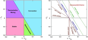
One rather nice way of viewing the various mixing mechanisms in stars is given in Figure 11, based on Figure 2 of Grossman & Taam (Reference Grossman and Taam1996). In the left panel we give the various stability criteria and the types of mixing that result, while the right panel also shows typical mixing speeds. In both panels the Schwarzschild stability criterion is given by the red line, and it predicts convection to the right of this red line. The blue line is the Ledoux criterion, with convection expected above the blue line. The green lines show expected velocities in the convective regions, while the brown lines show the dramatically reduced velocities expected for thermohaline or semi-convective mixing. For a general hydrodynamic formulation that includes both thermohaline mixing and semi-convection we refer the reader to Spiegel (Reference Spiegel1972) and Grossman et al. (Reference Grossman, Narayan and Arnett1993), and the series of papers by Canuto (Canuto Reference Canuto2011a, Reference Canuto2011b, Reference Canuto2011c, Reference Canuto2011d, Reference Canuto2011e).

Figure 11.

These diagrams show the main stability criteria for stellar models, the expected kind of mixing, and typical velocities. The left panel shows the Schwarzschild criterion as a red line, with convection expected to the right of the red line. The Ledoux criterion is the blue line, with convection expected above this line. The green region shows where the material is stable according to the Ledoux criterion but unstable according to the Schwarzschild criterion: this is semiconvection. The magenta region shows that although formally stable, mixing can occur if the gradient of the molecular weight is negative. The bottom left region is stable with no mixing. The right panel repeats the two stability criteria and also gives typical velocities in the convective regime (green lines) as well as the thermohaline and semi-convective regions (the brown lines). This figure is based on Figure 2 in Grossman & Taam (Reference Grossman and Taam1996).

Ulrich (Reference Ulrich1972) developed a one-dimensional theory for thermohaline mixing that was cast in the form of a diffusion co-efficient for use in stellar evolution calculations. This assumed a perfect gas equation of state but was later generalised by Kippenhahn, Ruschenplatt, & Thomas (Reference Kippenhahn, Ruschenplatt and Thomas1980). These two formulations are identical and rely on a single parameter C which is related to the assumed aspect ratio α of the resulting fingers via C = 8/3π²α² (Charbonnel & Zahn Reference Charbonnel and Zahn2007b).

The relevance of thermohaline mixing for our purposes follows from the work of Eggleton et al. (Reference Eggleton, Dearborn and Lattanzio2006). They found that a μ inversion developed naturally during the evolution along the RGB. During main sequence evolution a low-mass star produces ³He at relatively low temperatures as a result of the pp chains. At higher temperatures, closer to the centre, the ³He is destroyed efficiently by other reactions in the pp chains. This situation is shown in the left panel of Figure 12, which shows the profile of ³He when the star leaves the main sequence. The abundance of ³He begins very low in the centre, rises to a maximum about mid-way out (in mass) and then drops back to the initial abundance at the surface. When the FDU begins it homogenises the composition profile, as we have seen earlier and as shown in the right panel of Figure 12, and this mixes a significant amount of ³He in the stellar envelope. When the H shell approaches the abundance discontinuity left by the FDU the first reaction to occur at a significant rate is the destruction of ³He, which is at an abundance that is orders of magnitude higher than the equilibrium value for a region involved in H burning. The specific reaction is

Figure 12.

Abundance profiles in a 0.8 M_⊙ model with Z = 0.00015 (see also Figure 9). The left panel shows a time just after core hydrogen exhaustion and the right panel shows the situation soon after the maximum inward penetration of the convective envelope. At this time the hydrogen burning shell is at m(r) ≈ 0.31 M_⊙ and the convective envelope has homogenised all abundances beyond m(r) ≈ 0.36 M_⊙. The initial ³He profile has been homogenised throughout the mixed region, resulting in an increase in the surface value, which is then returned to the interstellar medium through winds, unless some extra-mixing process can destroy it first.

which completes the fusion of He. This reaction is unusual in that it actually increases the number of particles per volume, starting with two particles and producing three. The mass is the same and the reaction reduces μ locally. This is a very small effect, and it is usually swamped by the other fusion reactions that occur in a H-burning region. But here, this is the fastest reaction and it rapidly produces a μ inversion. This should initiate mixing. Further, it occurs just as the H shell approaches the discontinuity in the composition left behind by the FDU, i.e., it occurs just at the position of the LF bump, in accord with (most) observations. This mechanism has many attractive features because it is based on well-known physics, occurs in all low-mass stars, and occurs at the required position on the RGB (Charbonnel & Zahn Reference Charbonnel and Zahn2007b; Eggleton, Dearborn, & Lattanzio Reference Eggleton, Dearborn and Lattanzio2008).

Having identified a mechanism it remains to determine how to model it. Eggleton et al. (Reference Eggleton, Dearborn and Lattanzio2006, Reference Eggleton, Dearborn and Lattanzio2008) preferred to try to determine a mixing speed from first principles, and try to apply that in a phenomenological way. Charbonnel & Zahn (Reference Charbonnel and Zahn2007b) preferred to use the existing theory of Ulrich (Reference Ulrich1972) and Kippenhahn et al. (Reference Kippenhahn, Ruschenplatt and Thomas1980). Both groups found that the mechanism had the desired features, in that it began to alter the surface abundances at the required observed magnitude, it reduced the C isotope ratio to the lower values observed, and it destroyed almost all of the ³He produced in the star, thus reconciling the predicted yields of ³He with observations (Eggleton et al. Reference Eggleton, Dearborn and Lattanzio2006; Lagarde et al. Reference Lagarde, Charbonnel, Decressin and Hagelberg2011, Reference Lagarde, Romano, Charbonnel, Tosi, Chiappini and Matteucci2012), provided the free parameter C was taken to be C ≈ 1 000. Further, mixing reduced the A(Li) values as required by observation and it also showed the correct variation in behaviour with metallicity, i.e., the final ¹²C/¹³C ratios were lower for lower metallicity (Eggleton et al. Reference Eggleton, Dearborn and Lattanzio2008; Charbonnel & Lagarde Reference Charbonnel and Lagarde2010).

An extensive study of thermohaline mixing within rotating stars was performed by Charbonnel & Lagarde (Reference Charbonnel and Lagarde2010). They found that thermohaline mixing was far more efficient at mixing than meridional circulation, a result also found by Cantiello & Langer (Reference Cantiello and Langer2010). Note that the latter authors did not find that thermohaline mixing was able to reproduce the observed abundance changes on the RGB, but this is entirely due to their choice of a substantially lower value of the free parameter C (see also Wachlin, Miller Bertolami, & Althaus Reference Wachlin, Miller Bertolami and Althaus2011). Cantiello & Langer (Reference Cantiello and Langer2010) also showed that thermohaline mixing can continue during core He burning as well as on the AGB, and Stancliffe et al. (Reference Stancliffe, Church, Angelou and Lattanzio2009) found that it was able to reproduce most of the observed properties of both C-normal and C-rich stars, for the ‘canonical’ value of C ≈ 1 000.

The interaction between rotation and thermohaline mixing is a subtle thing, yet both Charbonnel & Lagarde (Reference Charbonnel and Lagarde2010) and Cantiello & Langer (Reference Cantiello and Langer2010) treated this crudely, by simply adding the separate diffusion coefficients. This is unlikely to be correct and one can easily imagine a situation where rotation, or any horizontal turbulence, could decrease the efficiency or even remove the thermohaline mixing altogether. Indeed a later study by Maeder et al. (Reference Maeder, Meynet, Lagarde and Charbonnel2013) showed that simple addition of the coefficients was not correct and these authors provide a formalism for simultaneously including multiple processes. Calculations using this scheme have not yet appeared in the literature.

For a more detailed comparison of predictions with data, Angelou et al. (Reference Angelou, Church, Stancliffe, Lattanzio and Smith2011, Reference Angelou, Stancliffe, Church, Lattanzio and Smith2012) decided to investigate the variation of [C/Fe] with absolute magnitude in GCs. The C isotopic ratio saturates quickly on the RGB, whereas [C/Fe] and [N/Fe] continue to vary along the RGB, providing information on the mixing over a wide range of luminosity. They found good agreement with the thermohaline mixing mechanism, again provided C ≈ 1 000, although they also noted that standard models failed to match the FDU found in the more metal-poor GCs, such as M92. This is not a failure of the thermohaline mixing paradigm but of the standard theory itself (as discussed earlier in Section 2.3.1).

Clearly the value of the free parameter C is crucial. On the one hand, it is gratifying that so many observational constraints are matched by a value of C ≈ 1 000. However, the value is not favoured a priori by some authors. We have seen that within the formalism of the idealised one-dimensional theory of Ulrich (Reference Ulrich1972) and Kippenhahn et al. (Reference Kippenhahn, Ruschenplatt and Thomas1980), the value of C is related to the aspect ratio α of the assumed ‘fingers’ doing the mixing, with C = 8/3π²α². If the mixing is more ‘blob-like’ than ‘finger-like’ then α ≈ 1 and C ≈ 20 rather than 1 000. This was the case preferred by Kippenhahn et al. (Reference Kippenhahn, Ruschenplatt and Thomas1980), in fact, whereas Ulrich (Reference Ulrich1972) preferred fingers with α ≈ 5 leading to C ≈ 700, much closer to the value of 1 000 that seems to fit so many constraints. We would caution against a literal interpretation of the aspect ratio and finger-like nature of the mixing. The one-dimensional theory is very idealised and we feel it is perhaps wise to remember that the diffusion equation is a convenient, rather than accurate, description of the mixing.

Even if we assume that the mechanism identified by Eggleton et al. (Reference Eggleton, Dearborn and Lattanzio2006) is the one driving extra mixing, it is unsatisfactory having an idealised, yet approximate, theory that still contains a free parameter. We need a detailed hydrodynamical understanding of the process. Studies along these lines have begun but a discussion of that would take us far afield from our main aim in this paper. We refer the reader to the following papers for details: Denissenkov, Pinsonneault, & MacGregor (Reference Denissenkov, Pinsonneault and MacGregor2009), Denissenkov (Reference Denissenkov2010), Denissenkov & Merryfield (Reference Denissenkov and Merryfield2011), Traxler, Garaud, & Stellmach (Reference Traxler, Garaud and Stellmach2011), Rosenblum et al. (Reference Rosenblum, Garaud, Traxler and Stellmach2011), Mirouh et al. (Reference Mirouh, Garaud, Stellmach, Traxler and Wood2012), and Brown, Garaud, & Stellmach (Reference Brown, Garaud and Stellmach2013). Let us summarise by saying that the models predict more blob-like structures, with low values of α and C values too small to match the observations. The stellar regime is difficult for simulations to model accurately and the final word is not yet written on the subject.

To summarise, thermohaline mixing occurs naturally at the appropriate magnitude on the RGB and it provides the right sort of mixing to solve many of the abundance problems seen on the RGB, as well as the ³He problem. One area where the thermohaline mechanism is open to criticism is its prediction that low-mass stars should almost completely destroy ³He and yet there are known planetary nebulae (PNe) with large amounts (i.e., consistent with the standard models) of ³He present, as pointed out by Balser, Rood, & Bania (Reference Balser, Rood and Bania2007, see also Guzman-Ramirez et al. Reference Guzman-Ramirez, Pineda, Zijlstra, Stancliffe and Karakas2013) immediately after the paper by Eggleton et al. (Reference Eggleton, Dearborn and Lattanzio2006). Charbonnel & Zahn (Reference Charbonnel and Zahn2007a) suggested that perhaps an explanation could be related to magnetic fields and identified the few percent of stars that do not show decreased C isotopic ratios with the descendants of Ap stars. They showed that remnant fields of order 10⁴ – 10⁵ Gauss, as expected from Ap stars when they become giants, are enough to inhibit thermohaline mixing.

2.3.5 Magnetic fields and other mechanisms

Despite its many appealing features, thermohaline mixing still suffers from at least one major problem: hydrodynamical models do not support the value of C required to match the observations. This leads to the search for other mechanisms.

One obvious contender is magnetic fields (Busso et al. Reference Busso, Wasserburg, Nollett and Calandra2007) produced by differential rotation just below the convective envelope. This can produce a toroidal field and mixing by magnetic buoyancy has been investigated by various authors (e.g., Nordhaus et al. Reference Nordhaus, Busso, Wasserburg, Blackman and Palmerini2008; Denissenkov et al. Reference Denissenkov, Pinsonneault and MacGregor2009).

In contrast, Denissenkov & Tout (Reference Denissenkov and Tout2000) suggested that a combination of meridional circulation and turbulent diffusion could produce the required mixing. These authors found that the rotation rates required were reasonable but we note that the best models of rotating stars at present do not produce enough mixing.

2.6.1 Curtailing first dredge-up

At metallicities of [Fe/H] ≲ −1, the evolution of post main sequence stars begins to significantly differ to that found in disk or near-solar metallicity stars. For intermediate-mass stars the necessary central temperatures for core He burning are reached while the star crosses the Hertzsprung gap. This means that the star will ignite He before evolving up the RGB and as a consequence will not experience the FDU (e.g., Boothroyd & Sackmann Reference Boothroyd and Sackmann1999; Marigo et al. Reference Marigo, Girardi, Chiosi and Wood2001). In Figure 13 we show evolutionary tracks for models of 3 M_⊙ at a metallicity of Z = 0.02 and Z = 0.0001, respectively. The lower metallicity model skips the RGB altogether. At a metallicity of Z = 0.001 or [Fe/H] ≈ −1.2 the upper mass limit that experiences the FDU is 3 M_⊙, by a metallicity of Z = 0.0001 or [Fe/H] ≈ −2.3, this mass has been reduced to 2.25 M_⊙, and even at that mass the maximum extent of the convective envelope only reaches a depth of ≈ 1 M_⊙ from the centre (compared to a Z = 0.02 model of 2.25 M_⊙ where the FDU reaches a depth of ≈ 0.35 M_⊙ from the stellar centre). Because the lower metallicity model is hotter and has a larger core during the main sequence the FDU still causes a 30% drop in the surface C abundance (compared to a drop of 36% for the Z = 0.02 model). For intermediate-mass stars that do not experience a FDU, the second dredge-up event, which takes place during the early ascent of the AGB, is the first mixing episode that changes the surface composition (Boothroyd & Sackmann Reference Boothroyd and Sackmann1999; Chieffi et al. Reference Chieffi, Domínguez, Limongi and Straniero2001; Marigo et al. Reference Marigo, Girardi, Chiosi and Wood2001; Karakas & Lattanzio Reference Karakas and Lattanzio2007; Campbell & Lattanzio Reference Campbell and Lattanzio2008).

Figure 13.

Hertzsprung–Russell (HR) diagram showing the evolutionary tracks for 3 M_⊙ models of Z = 0.02 (black solid line) and Z = 0.0001 (red dashed line). The low-metallicity model is hotter and brighter at all evolutionary stages and does not experience a RGB phase or the first dredge-up.

2.6.2 The core helium flash

Metallicity has an important consequence for stars that experience the core He flash. Evolution at lower metallicities is hotter, owing to a lower opacity. This means that the stars experience a shorter time on the RGB before reaching temperatures for core He ignition and therefore do not become as electron degenerate. This means that the maximum mass for the core He flash decreases with decreasing Z (Marigo et al. Reference Marigo, Girardi, Chiosi and Wood2001). We mentioned previously that at solar metallicity the maximum mass for the core He flash is 2.1 M_⊙, whereas at [Fe/H] = − 2.3 the maximum mass is 1.75 M_⊙, with the 2 M_⊙ model experiencing a fairly quiescent He ignition with only a moderate peak in the He luminosity (Karakas & Lattanzio Reference Karakas and Lattanzio2007; Karakas Reference Karakas2010).

There is now a fairly extensive literature on multi-dimensional studies of the core He flash (Deupree Reference Deupree1984, Reference Deupree1986; Deupree & Wallace Reference Deupree and Wallace1987; Deupree Reference Deupree1996; Dearborn et al. Reference Dearborn, Lattanzio and Eggleton2006; Mocák et al. Reference Mocák, Müller, Weiss and Kifonidis2009). Early results from two-dimensional hydrodynamic simulations (Deupree & Wallace Reference Deupree and Wallace1987) suggest that the flash could be a relatively quiescent or violent hydrodynamic event, depending on the degeneracy of the stellar model. Deupree (Reference Deupree1996) finds for low-mass solar composition models, using improved but still uncertain input physics, that the core flash is not a violent hydrodynamic event and that there is no mixing between the flash-driven H-exhausted core and the envelope at this metallicity. More recent multi-dimensional hydrodynamic simulations of the core He flash in metal-free stars find that the He-burning convection zone moves across the entropy barrier and reaches the H-rich layers (Mocák et al. Reference Mocák, Campbell, Müller and Kifonidis2010; Mocák, Siess, & Müller Reference Mocák, Siess and Müller2011).

For the present we assume that stars experiencing the core He flash do not mix any products into their envelope. This is in accord with standard models and the observations do not disagree. We do note that this is not necessarily true at lower metallicity, as we discuss in the next section.

2.6.3 Proton ingestion episodes

The low entropy barrier between the He- and H-rich layer can lead to the He flash-driven convective region penetrating the inner edge of the (now extinguished) H-burning shell. If this happens, protons will be ingested into the hot core during the core He flash. If enough protons are ingested, a concurrent secondary flash may occur that is powered by H burning and gives rise to further nucleosynthesis in the core. The subsequent dredge-up of matter enriches the stellar surface with large amounts of He, C, N, and even possibly heavy elements synthesised by the s process. There has been an extensive number of studies of the core He flash and resulting nucleosynthesis in low-mass, very metal-poor stars (e.g., D’Antona & Mazzitelli Reference D’Antona and Mazzitelli1982; Fujimoto, Iben, & Hollowell Reference Fujimoto, Iben and Hollowell1990; Hollowell, Iben, & Fujimoto Reference Hollowell, Iben and Fujimoto1990; Schlattl et al. Reference Schlattl, Cassisi, Salaris and Weiss2001; Picardi et al. Reference Picardi, Chieffi, Limongi, Pisanti, Miele, Mangano and Imbriani2004; Weiss et al. Reference Weiss, Schlattl, Salaris and Cassisi2004; Suda, Fujimoto, & Itoh Reference Suda, Fujimoto and Itoh2007; Campbell & Lattanzio Reference Campbell and Lattanzio2008; Suda & Fujimoto Reference Suda and Fujimoto2010; Campbell, Lugaro, & Karakas Reference Campbell, Lugaro and Karakas2010). The details of the input physics used in the calculations clearly matter, where the low-mass Z = 0 models of Siess, Livio, & Lattanzio (Reference Siess, Livio and Lattanzio2002) find no mixing between the flash-driven convective region and the overlying H-rich layers. It has been known for some time that the treatment of the core He flash in one-dimensional stellar evolutionary codes is approximate at best, owing to the fact that the core He flash is a multi-dimensional phenomenon (Deupree Reference Deupree1996; Mocák et al. Reference Mocák, Siess and Müller2011). We deal more extensively with this in Section 3.8.

3.2.1 Dredge-up, HBB and the brightest C stars

Third dredge-up can continue after the cessation of HBB, which allows the C abundance to increase instead of being burnt to N. The envelope mass is relatively small at this stage (≲ 1 M_⊙), which means that dilution is also lower. It is possible the star will become C-rich at the very tip of the AGB where C/O ⩾ 1 (Frost et al. Reference Frost, Cannon, Lattanzio, Wood and Forestini1998a), depending on the number of TDU episodes after the end of HBB and the O abundance in the envelope (noting that some O can also be destroyed by HBB). van Loon, Zijlstra, & Groenewegen (Reference van Loon, Zijlstra and Groenewegen1999b) presented observational evidence that supports this scenario, finding a sample of very luminous, dust-obscured AGB stars in the Magellanic Clouds. The existence of very bright, C-rich AGB stars is also evidence that stars in this mass range experience TDU, at least down to the metallicities of the Magellanic Clouds.

3.2.2 The core-mass vs. luminosity relation

The surface luminosity will reach a maximum value during the interpulse and this is reached just before the onset of the next thermal pulse. Paczyński (Reference Paczyński1970) was the first to derive a linear relationship between the maximum surface luminosity during the quiescent interpulse phase and the H-exhausted core mass:

Paczyński’s calculations infer that there is a maximum luminosity an AGB model can have of 52 021 L_⊙, determined by the maximum possible core mass of ≈ 1.4 M_⊙. Subsequent calculations of intermediate-mass AGB stars revealed that hot bottom burning can violate the conditions of the core-mass luminosity relationship (Blöcker & Schoenberner Reference Blöcker and Schoenberner1991; Lattanzio Reference Lattanzio1992; Boothroyd & Sackmann Reference Boothroyd and Sackmann1992) and that an AGB model can have luminosities larger than predicted by Paczyński. The core-mass luminosity relationship on the AGB is also a key ingredient in a synthetic AGB model because it determines many fundamental features of AGB evolution including the growth of the H-exhausted core with time. The most accurate fits to the core-mass luminosity relationship are those that include a correction for the extra luminosity provided by HBB (Wagenhuber & Groenewegen Reference Wagenhuber and Groenewegen1998; Izzard et al. Reference Izzard, Tout, Karakas and Pols2004, Reference Izzard, Dray, Karakas, Lugaro and Tout2006). In Figure 18 we show the core-mass luminosity relationship for a selection of models at Z = 0.02. HBB occurs in models with M ⩾ 4.5 M_⊙ at Z = 0.02 and we can see for these models that the luminosity strongly increases with core mass before peaking and then declining. The decline is caused by mass loss, which reduces the temperature at the base of the convective envelope and in turn the luminosity from the CN cycle. In comparison, the lower mass AGB models do not experience HBB and show a reasonably linear core-mass luminosity relationship.

Figure 18.

The core-mass versus luminosity relationship for a selection of Z = 0.02 models between 2 M_⊙ and 7 M_⊙. The models with M ⩾ 4.5 M_⊙ have hot bottom burning and deviate from the Paczyński relation, shown by the solid black line.

3.3.1 The dredge-up parameter

If there is dredge-up, then a fraction of the outer-most part of the H-exhausted core will be mixed into the envelope according to

where λ is the third dredge-up efficiency parameter, ΔM _dredge is the mass mixed into the envelope, and ΔM _core is the amount by which the H-exhausted core increases over the previous interpulse phase; see Figure 19. From the above definition, when λ = 1, the core mass does not grow from pulse to pulse but remains constant. The value of λ depends on physical parameters such as the core mass and metallicity of the star. Exactly how λ depends on these quantities is unknown and reflects our lack of understanding about how convection operates in stellar interiors. Different stellar codes predict different behaviour, a point we will come back to in Section 4.1. Note that there is no a priori reason why λ cannot exceed unity.

Figure 19.

The definition of λ, shown schematically, where the x–axis represents time and the y–axis represents the mass of the H-exhausted core.

So in summary, AGB nucleosynthesis depends on

1. 1. λ, the efficiency of third dredge-up;

2. 2. M ^min _c, the minimum core mass at which the TDU begins; this determines how many TDU episodes will occur before mass loss removes the envelope;

3. 3. the size of the convective envelope, which sets the level of dilution of each TDU episode;

4. 4. the mass of the He intershell.

Karakas et al. (Reference Karakas, Lattanzio and Pols2002) provided the first parameterisation of λ and M ^min _c as functions of the total mass, envelope mass, and metallicity (see also Straniero et al. Reference Straniero, Domínguez, Cristallo and Gallino2003a). The general trend is that λ increases with increasing stellar mass, at a given Z. The parameter λ also increases with decreasing metallicity, at a given mass (e.g., Boothroyd & Sackmann Reference Boothroyd and Sackmann1988). Naively, this means that it should be easier to make C stars in lower metallicity or higher mass models. But there is also a second reason why C stars are more easily made at lower metallicity. Carbon production is a primary product of the triple-α process, and hence the C intershell abundance does not depend on the global metallicity, Z. In a low-metallicity star the amount of C added per pulse is roughly independent of metallicity, whereas the amount of O that must be overcome to produce C > O is lower. So fewer pulses are required to make a C star. This is true even for α-enhanced compositions where [O/Fe] ≈ +0.4. As we note, stars of lower metallicity are predicted to have deeper dredge-up which accelerates the effect further. Both mechanisms act to make C-stars easier to form at lower metallicities.

For intermediate-mass stars the situation is more complex. Even though the calculations of Karakas et al. (Reference Karakas, Lattanzio and Pols2002) predict larger values of λ, the effect of TDU is mitigated by the mass of the He intershell which is approximately a factor of 10 smaller in intermediate-mass AGB stars compared to AGB stars of lower mass. This means that even if λ ≈ 0.9, the amount of material added to the envelope per TDU event (λ × ΔM _core) is smaller by about an order of magnitude. Second, the mass of the convective envelope is large in intermediate-mass stars, which means that the material will be more diluted. Finally, HBB will act to prevent the formation of C-rich luminous AGB stars at the highest metallicities (e.g., Karakas et al. Reference Karakas, García-Hernández and Lugaro2012), which is in agreement with observations of O-rich luminous AGB stars in our Galaxy (García-Hernández et al. Reference García-Hernández, García-Lario, Plez, D’Antona, Manchado and Trigo-Rodríguez2006, Reference García-Hernández, Zamora, Yagüe, Uttenthaler, Karakas, Lugaro, Ventura and Lambert2013). So even though the conventional wisdom is that C-star production does not happen at intermediate-mass for the above reason, calculations of low-metallicity (Z ⩽ 0.001) intermediate-mass stars suggest that C-star formation will occur before HBB ceases (Herwig Reference Herwig2004a, Reference Herwig2004b; Karakas Reference Karakas2010; Lugaro et al. Reference Lugaro, Karakas, Stancliffe and Rijs2012; Fishlock, Karakas, & Stancliffe Reference Fishlock, Karakas and Stancliffe2014; Straniero, Cristallo, & Piersanti Reference Straniero, Cristallo and Piersanti2014). This is driven by the combination of primary C production plus the effect of HBB destroying some O.

It is important to know if the stellar models are providing an accurate description of the efficiency of mixing in AGB stars. For example, the models of Karakas et al. (Reference Karakas, Lattanzio and Pols2002) do not predict any TDU for models less than 2 M_⊙ at Z = 0.02 and quite efficient TDU for models of intermediate mass. While it is notoriously difficult to determine the masses of stars in our Galaxy, observations suggest that the minimum initial stellar mass for C-star formation is ≈ 1.5 M_⊙ (Wallerstein & Knapp Reference Wallerstein and Knapp1998). The Large and Small Magellanic Clouds (LMC, SMC, respectively) are the closest satellite galaxies of our Milky Way and they both have thousands of known C stars (Frogel, Mould, & Blanco Reference Frogel, Mould and Blanco1990; Groenewegen Reference Groenewegen2004). We know the distances to these two galaxies reasonably well, enabling us to construct C-star luminosity functions (CSLFs).

3.3.2 The carbon star luminosity function and other observational constraints

Is it possible to constrain the efficiency of third dredge-up by using the CSLF of the LMC and the SMC? That the stellar luminosity on the AGB is a nearly linear function of the H-exhausted core mass (e.g., Equation (1) and Figure 18) has stimulated the development of synthetic AGB evolution models, as a quick way of simulating populations of AGB stars. The main observational constraint which models must face is the CSLF for the Magellanic Clouds.

Synthetic AGB evolution calculations performed by Groenewegen & de Jong (Reference Groenewegen and de Jong1993) and Marigo, Bressan, & Chiosi (Reference Marigo, Bressan and Chiosi1996) treat λ as a constant free parameter, calibrated by comparison with the CSLF. Synthetic AGB calculations designed to reproduce the CSLF in the LMC and SMC require an average λ = 0.5 and λ = 0.65 respectively, and M ^min _c ≈ 0.58 M_⊙ (Groenewegen & de Jong Reference Groenewegen and de Jong1993; Marigo, Girardi, & Bressan Reference Marigo, Girardi and Bressan1999; Izzard et al. Reference Izzard, Tout, Karakas and Pols2004; Marigo & Girardi Reference Marigo and Girardi2007). The values for M ^min _c are lower than found in detailed models by e.g., Karakas et al. (Reference Karakas, Lattanzio and Pols2002) and shown in Figure 20 and the synthetic best fit values for λ are higher than those found for the low-mass AGB models that become C-rich (e.g., λ ≲ 0.4 in Figure 20) unless considerable overshoot is applied (e.g., Herwig Reference Herwig2000; Cristallo et al. Reference Cristallo, Straniero, Gallino, Piersanti, Domínguez and Lederer2009; Weiss & Ferguson Reference Weiss and Ferguson2009).

Figure 20.

The minimum core mass for TDU (upper panel) and the maximum value of λ plotted against initial mass for the Z = 0.008 models from Karakas et al. (Reference Karakas, Lattanzio and Pols2002). Only models with M ⩾ 1.9 M_⊙ become C-rich. Figure taken from Karakas et al. (Reference Karakas, Lattanzio and Pols2002).

Stancliffe, Izzard, & Tout (Reference Stancliffe, Izzard and Tout2005) were able to reproduce the CSLF of the LMC by computing AGB models without convective overshoot using the Cambridge STARS code, which predicts deeper TDU at smaller core masses than Straniero et al. (Reference Straniero, Chieffi, Limongi, Busso, Gallino and Arlandini1997) or Karakas et al. (Reference Karakas, Lattanzio and Pols2002). However, the CSLF in the SMC cannot be reproduced from detailed STARS models, indicating that the problem is not yet fully solved.

Star clusters are ideal sites to constrain the TDU in AGB stars as they contain stars of similar age and metallicity. Open clusters of solar metallicity in the Milky Way Galaxy can be used to study the TDU and the growth of the core using observations of white dwarf masses in comparison to theoretical models (Kalirai, Marigo, & Tremblay Reference Kalirai, Marigo and Tremblay2014). Star clusters in the Magellanic Clouds in particular prove very valuable as they span a wide range of age, which enables us to study the evolution of stars with masses around 1.5 to 5 M_⊙ (e.g., Girardi et al. Reference Girardi, Chiosi, Bertelli and Bressan1995; Girardi, Rubele, & Kerber Reference Girardi, Rubele and Kerber2009; Maceroni et al. Reference Maceroni, Testa, Plez, García Lario and D’Antona2002; Mucciarelli et al. Reference Mucciarelli, Origlia, Ferraro, Maraston and Testa2006; Mackey et al. Reference Mackey, Broby Nielsen, Ferguson and Richardson2008; Milone et al. Reference Milone, Bedin, Piotto and Anderson2009).

The clusters NGC 1978 and NGC 1846 in the LMC have been the subject of much study owing to the availability of accurate estimates of AGB structural parameters such as pulsation masses, effective temperatures, and luminosity. Kamath et al. (Reference Kamath, Wood, Soszyński and Lebzelter2010) obtained (current day) pulsation masses for NGC 1978 (and the SMC cluster NGC 419), while Lebzelter & Wood (Reference Lebzelter and Wood2007) obtained masses for the LMC cluster NGC 1846. Abundance studies have also been done (Ferraro et al. Reference Ferraro, Mucciarelli, Carretta and Origlia2006; Mucciarelli et al. Reference Mucciarelli, Carretta, Origlia and Ferraro2008; Lebzelter et al. Reference Lebzelter, Lederer, Cristallo, Hinkle, Straniero and Aringer2008; Lederer et al. Reference Lederer, Lebzelter, Cristallo, Straniero, Hinkle and Aringer2009), along with attempts to explain the observed C and O abundances for NGC 1978 and NGC 1846 using stellar evolution models (Lebzelter et al. Reference Lebzelter, Lederer, Cristallo, Hinkle, Straniero and Aringer2008; Lederer et al. Reference Lederer, Lebzelter, Cristallo, Straniero, Hinkle and Aringer2009).

Kamath et al. (Reference Kamath, Karakas and Wood2012) presented stellar models for AGB stars in NGC 1978, NGC 1846, and NGC 419 with the aim of constraining the TDU and mass loss on the AGB. The stellar evolution models were constrained to reflect the observed AGB pulsation mass, cluster metallicity, giant branch effective temperature, M-type to C-type transition luminosity, and the AGB-tip luminosity. A major finding from the study by Kamath et al. (Reference Kamath, Karakas and Wood2012) is that a large amount of convective overshoot (up to 3 pressure scale heights) is required at the base of the convective envelope during third dredge-up in order to get the correct O-rich to C-rich transition luminosity. Such large overshoot leads to λ values in the range 0.66 to 0.82 for the best fitting models. The first shell flashes with dredge-up occur for core masses of M ^min _c ≈ 0.56 − 0.58 M_⊙. These values are much closer to the those values above suggested by synthetic AGB models to fit CSLFs and suggest that considerable convective overshoot occurs in low-mass AGB stars (see also studies by Herwig et al. Reference Herwig, Bloecker, Schoenberner and El Eid1997; Herwig Reference Herwig2000; Cristallo et al. Reference Cristallo, Straniero, Gallino, Piersanti, Domínguez and Lederer2009; Weiss & Ferguson Reference Weiss and Ferguson2009; Karakas et al. Reference Karakas, Campbell and Stancliffe2010).

It is important to note that this overshoot is measured from the formal Schwarzschild boundary. We know that this point is unstable to growth, but it does form a convenient position from which to measure the required amount of overshoot. Knowing the Schwarzschild boundary to be unstable has motivated some authors to implement an algorithm to try to search for a neutrally stable point (e.g., Lattanzio Reference Lattanzio1986). We note that this was not able to reproduce the observations in Kamath et al. (Reference Kamath, Karakas and Wood2012), and further mixing was required (although the required depth was not compared to the position of the neutral point).

The large spread in the amount of overshoot required to match the observations could be telling us that is not the best way to quantify the required deeper mixing. It may indicate a mass dependence, with lower masses requiring deeper mixing. It is good to remember that although we call this ‘overshoot’ because it is mixing beyond the Schwarzschild boundary, we are not identifying the cause of the deeper mixing as ‘convective overshoot’ in the usual sense, that is to say, the mixing caused by conservation of momentum in the moving gas, which causes it to cross the point of zero acceleration (the Schwarzschild boundary). Rather, we mean any process that mixes beyond the Schwarzschild border.

3.5.1 The carbon isotopic ratio: ¹²C/¹³C

The C isotope ratio ¹²C/¹³C is a useful probe of AGB nucleosynthesis. Dredge-up increases the amount of ¹²C, so the ratio will increase from ¹²C/¹³C ≈ 10 − 20 at the tip of the RGB to between 30 and > 100, depending on the number of TDU episodes and the initial mass. For the 3 M_⊙ model star the predicted ¹²C/¹³C ratio goes from ≈ 20 before the AGB to 119 at the tip of the AGB.

The ¹²C/¹³C ratio has been observed in samples of C-rich AGB stars (Lambert et al. Reference Lambert, Gustafsson, Eriksson and Hinkle1986; Abia & Isern Reference Abia and Isern1997) as well as PNe (Palla et al. Reference Palla, Bachiller, Stanghellini, Tosi and Galli2000; Rubin et al. Reference Rubin, Ferland, Chollet and Horstmeyer2004). The C isotopic composition of pre-solar mainstream silicon carbide (SiC) grains, which are assumed to form in the extended envelopes of C-rich AGB stars, show a well-defined distribution where 40 ≲ ¹²C/¹³C ≲ 100, which matches the ratios observed in C(N) stars (e.g., Zinner Reference Zinner1998).

The ¹²C/¹³C ratios are difficult to measure in PNe, with values spanning the range from ~ 4, the equilibrium value of the CN cycle, to upper limits of ≈ 38 (Palla et al. Reference Palla, Bachiller, Stanghellini, Tosi and Galli2000, Reference Palla, Galli, Marconi, Stanghellini and Tosi2002; Rubin et al. Reference Rubin, Ferland, Chollet and Horstmeyer2004). These ratios are, in general, lower than measured in C-rich AGB stars and lower than found in pre-solar SiC grains and suggest efficient mixing of H-burning material with the observed nebula. Atacama large millimeter/sub-millimeter array (ALMA) observations of R Sculptoris however show the surprising result that the ¹²C/¹³C ratio at the stellar photosphere is much lower, at 19, compared to the ratio obtained in the present-day mass loss (≳ 60; Vlemmings et al. Reference Vlemmings2013). These authors speculate that the lower C isotopic ratio is due to an embedded source of UV-radiation that is primarily photo-dissociating the ¹³CO molecule. This suggests that we need to be wary of the ratios obtained from PNe, where the star is a strong UV source illuminating the nebula.

The C and N abundances predicted by models do not match those observed in AGB stars (e.g., Lambert et al. Reference Lambert, Gustafsson, Eriksson and Hinkle1986; Abia & Isern Reference Abia and Isern1997; Milam, Woolf, & Ziurys Reference Milam, Woolf and Ziurys2009). In particular the observed ¹²C/¹³C ratios are lower than predicted by standard AGB models (e.g., Forestini & Charbonnel Reference Forestini and Charbonnel1997; Cristallo et al. Reference Cristallo, Straniero, Gallino, Piersanti, Domínguez and Lederer2009; Karakas Reference Karakas2010). For example, standard AGB models predict that by the time C/O ⩾ 1 then ¹²C/¹³C ⩾ 80, which is already close to the upper limit observed in AGB stars or measured in SiC grains.

It is possible to match the observed N and C isotopic ratios by artificially lowering the ¹²C/¹³C ratio at the tip of the RGB to values observed in RGB stars (Kahane et al. Reference Kahane, Dufour, Busso, Gallino, Lugaro, Forestini and Straniero2000; Lebzelter et al. Reference Lebzelter, Lederer, Cristallo, Hinkle, Straniero and Aringer2008; Karakas et al. Reference Karakas, Campbell and Stancliffe2010; Kamath et al. Reference Kamath, Karakas and Wood2012). By adopting a ¹²C/¹³C ratio of 12 at the tip of the RGB, Kahane et al. (Reference Kahane, Dufour, Busso, Gallino, Lugaro, Forestini and Straniero2000) found that they could match the observed ¹²C/¹³C ratio of 45 for CW Leo. Similarly Karakas et al. (Reference Karakas, Campbell and Stancliffe2010) were able to reproduce the observed ¹²C/¹³C ratios for most of the Galactic C-rich stars. Whereas most C-rich AGB stars have ¹²C/¹³C ratios between about 30 and 80, there is a small number with ¹²C/¹³C ratios below 30 (e.g., Lambert et al. Reference Lambert, Gustafsson, Eriksson and Hinkle1986; Abia & Isern Reference Abia and Isern1997) that cannot be explained using the method above. That is, for a minimum ¹²C/¹³C ratio of 10 at the tip of the RGB the minimum predicted value at the tip of the AGB is about 30 (depending on mass and composition). A value lower than this will require some form of extra mixing on the AGB.

3.5.2 Nitrogen isotopic ratios

Nitrogen isotopic measurements have been made for a small number of evolved stars. Measurements were made for the cool C star IRC + 10216, where the ¹⁴N/¹⁵N ratio was estimated at > 4 400 (Guelin et al. Reference Guelin, Forestini, Valiron, Ziurys, Anderson, Cernicharo and Kahane1995; Kahane et al. Reference Kahane, Dufour, Busso, Gallino, Lugaro, Forestini and Straniero2000). A tentative value of ≈ 150 was made for the J-type star Y CVn (Olson & Richter Reference Olson and Richter1979), and lower limits (along with two detections) were obtained in eight C stars and two proto-PNe (Wannier et al. Reference Wannier, Andersson, Olofsson, Ukita and Young1991). In this last study six of the lower limits (> 500) were significantly larger than the ratio found in giant molecular clouds (330). Note that the Wannier et al. (Reference Wannier, Andersson, Olofsson, Ukita and Young1991) ¹⁴N/¹⁵N abundance ratio for Y CVn is 70, and for IRC + 10216 it is 5 300.

The most recent measurements by Hedrosa et al. (Reference Hedrosa, Abia, Busso, Cristallo, Domínguez, Palmerini, Plez and Straniero2013) were made for a selection of AGB stars of type C, SC, and J, where J-type C stars are defined mainly by their low ¹²C/¹³C ratio and by the absence of s-process elements (Wallerstein & Knapp Reference Wallerstein and Knapp1998). While almost all the data for C-type AGB stars show ¹⁴N/¹⁵N ≳ 1 000, a few C-type AGB stars have N isotopic values close to solar. These are difficult to reconcile with current models because known mixing events either increase the ¹⁴N/¹⁵N ratio by mixing with regions that have experienced H burning (e.g., FDU, SDU with typical values shown in Table 1 and extra mixing) or leave it largely unchanged because the material mixed to the surface is not primarily from H-burning regions (e.g., TDU). Furthermore, some of the SC type AGB stars, which are defined by having C/O ≈ 1, and presumably on an evolutionary path that takes them from M-type (O-rich) to C-type (C-rich) should have N isotopic ratios similar to C-type AGB stars. Instead, Hedrosa et al. (Reference Hedrosa, Abia, Busso, Cristallo, Domínguez, Palmerini, Plez and Straniero2013) find the SC-type AGB stars to be ¹⁵N-rich (with ¹⁴N/¹⁵N ≲ 1 000), regardless of their C isotopic ratios. The reason for this deviation between SC and C-type AGB stars is unclear and difficult to understand from a theoretical viewpoint. Furthermore, the J-type stars, whose origin is already a mystery, show ¹⁴N/¹⁵N ratios ≲ 1 000. The origin of the ¹⁵N enrichments is not clear but the only way that this isotope can be produced in low-mass AGB stars is via the CNO cycle reaction ¹⁸O(p,α)¹⁵N, which can take place in the He-burning shell provided there is a supply of protons (as discussed below in the context of F production).

3.5.3 The intershell oxygen abundance

The short duration of thermal pulses and the low C content of the region means that the ¹²C(α, γ)¹⁶O reaction produces negligible energy and does not produce much ¹⁶O. Canonical stellar evolution calculations of AGB stars find ¹⁶O intershell compositions of ≲ 2% (by mass, e.g., Boothroyd & Sackmann Reference Boothroyd and Sackmann1988; Karakas et al. Reference Karakas, Campbell and Stancliffe2010). Here by ‘canonical’ we are referring to model calculations with no convective overshoot of the flash-driven convective pocket into the C–O core. Herwig (Reference Herwig2000) does include convective overshoot at the inner border of the flash driven convective zone and finds that some C and O from the C–O core is mixed into the intershell. This has the effect of increasing the C and O intershell abundances to up to ≈ 40% and 20%, respectively. The inclusion of such overshoot means that the oxygen stellar yields from low-mass AGB stars may become significant (Pignatari et al. Reference Pignatari2013). We discuss this further in Section 3.5.7.

3.5.4 Fluorine

Fluorine is produced through a complex series of reactions as outlined in detail by Forestini et al. (Reference Forestini, Goriely, Jorissen and Arnould1992), Mowlavi, Jorissen, & Arnould (Reference Mowlavi, Jorissen and Arnould1996), Mowlavi, Jorissen, & Arnould (Reference Mowlavi, Jorissen and Arnould1998) and more recently by Lugaro et al. (Reference Lugaro, Ugalde, Karakas, Görres, Wiescher, Lattanzio and Cannon2004). The main reaction pathway involves the production of ¹⁵N which is burnt to ¹⁹F via ¹⁵N(α,γ)¹⁹F. The difficulty here is in making ¹⁵N which is destroyed by proton captures in the CNO cycles, which means that the composition of the He shell before a thermal pulse will be almost devoid of this isotope. If protons can be produced by secondary reactions (e.g., ¹⁴N(n,p)¹²C which itself requires free neutrons) then the CNO chain reaction ¹⁸O(p,α)¹⁵N can make ¹⁵N. Because F is produced in the He intershell the composition in the envelope correlates with the abundance of C and s-process elements, as shown in Figure 22 (for C).

Figure 22.

The C/O ratio versus the [F/Fe] abundance at the surface of a 3 M_⊙, Z = 0.02 AGB model. Other products of helium nucleosynthesis include ²²Ne, and the final ²²Ne/Ne ratio in this model increases to ≈ 0.4 from 0.068 initially. The total Ne abundance increases from log ε(Ne) = log ₁₀(Ne/H) + 12 = 8.11 at the main sequence to 8.33 at the tip of the AGB where He/H = 0.119, C/O = 1.74 (shown in Figure 21), ¹²C/¹³C = 119, ¹⁴N/¹⁵N ≈ 2 500, and N/O = 0.40.

Fluorine has been observed in AGB stars in our Galaxy and in Local Group Galaxies (Jorissen, Smith, & Lambert Reference Jorissen, Smith and Lambert1992; Lebzelter et al. Reference Lebzelter, Lederer, Cristallo, Hinkle, Straniero and Aringer2008; Abia et al. Reference Abia, Recio-Blanco, de Laverny, Cristallo, Domínguez and Straniero2009, Reference Abia2010), PG 1159 post-AGB stars and PNe (Werner, Rauch, & Kruk Reference Werner, Rauch and Kruk2005; Otsuka et al. Reference Otsuka, Izumiura, Tajitsu and Hyung2008), and in barium stars (Alves-Brito et al. Reference Alves-Brito, Karakas, Yong, Meléndez and Vásquez2011), which are hypothesised to have received their C and Ba through mass transfer from a previous AGB companion.

The observations of Jorissen et al. (Reference Jorissen, Smith and Lambert1992) revealed F abundances that were much higher than model predictions (Forestini et al. Reference Forestini, Goriely, Jorissen and Arnould1992; Lugaro et al. Reference Lugaro, Ugalde, Karakas, Görres, Wiescher, Lattanzio and Cannon2004; Karakas et al. Reference Karakas, Lee, Lugaro, Görres and Wiescher2008), especially for the SC-type AGB stars with C/O ≈ 1. A re-analysis of the F abundance in three Galactic AGB stars (TX Psc, AQ Sgr, and R Scl) by Abia et al. (Reference Abia2010) revealed the cause of the discrepancy to be the model atmospheres used in the original analysis, which did not properly take into account blending with C-bearing molecules. The new abundances are up to 0.8 dex lower, bringing the models into agreement with the observations. Observations of F in the C-rich AGB stars in the LMC cluster NGC 1846 however show a discrepancy with models (Lebzelter et al. Reference Lebzelter, Lederer, Cristallo, Hinkle, Straniero and Aringer2008; Kamath et al. Reference Kamath, Karakas and Wood2012), with the observed F abundance increasing more strongly with the C/O ratio than in the theoretical model. While observations of F in extra-galactic C stars show most of the stars to be F rich, the models over predict the amount of C relative to the observations; see Abia et al. (Reference Abia, Cunha, Cristallo, de Laverny, Domínguez, Recio-Blanco, Smith and Straniero2011), who also suggested possible solutions including the hypothesis that most of the C might be trapped in dust grains.

3.5.5 Other species in the intershell

There is a wealth of other He-burning products produced as a consequence of thermal pulses including ¹⁹F, ²²Ne, ²³Na, ²⁵Mg, ²⁶Mg, and ²⁷Al (Forestini & Charbonnel Reference Forestini and Charbonnel1997; Mowlavi Reference Mowlavi1999b; Herwig Reference Herwig2000; Karakas & Lattanzio Reference Karakas and Lattanzio2003a, Reference Karakas and Lattanzio2003b; Lugaro et al. Reference Lugaro, Ugalde, Karakas, Görres, Wiescher, Lattanzio and Cannon2004; Cristallo et al. Reference Cristallo, Straniero, Gallino, Piersanti, Domínguez and Lederer2009; Karakas Reference Karakas2010; Cristallo et al. Reference Cristallo2011). The isotope ²²Ne is produced by the reaction ¹⁴N(α, γ)¹⁸F, where ¹⁸F β-decays to ¹⁸O allowing for the reaction ¹⁸O(α, γ)²²Ne. The composition of ²²Ne in the intershell is fairly high, at ≈ 2%. This is because the abundant ¹⁴N is completely converted into ²²Ne during a thermal pulse. The ²²Ne abundance is predicted to increase by almost an order of magnitude (~ 1 dex) in some AGB models (Karakas & Lattanzio Reference Karakas and Lattanzio2003a). If the ²²Ne abundance exceeds or is equal to the ²⁰Ne abundance we should expect an observable enhancement in the elemental Ne composition. The intershell is also enriched in ²³Na and ²⁷Al. Na and ²⁷Al are not He-burning products but are synthesised in the H shell during the previous interpulse. Unlike other H-burning products (e.g., ¹⁴N) these are left unburnt by the subsequent TP and mixed into the envelope by the next TDU episode.

3.5.6 Heavy magnesium isotopes

If the peak temperature of the thermal pulse exceeds 300 × 10⁶ K, the neutron-rich Mg isotopes, ²⁵Mg and ²⁶Mg, can be synthesised by the ²²Ne(α, n)²⁵Mg and ²²Ne(α, γ)²⁶Mg reactions. These two ²²Ne + α reactions have similar although uncertain rates at He-shell burning temperatures (Angulo et al. Reference Angulo1999; Karakas et al. Reference Karakas, Lugaro, Wiescher, Goerres and Ugalde2006b; Longland, Iliadis, & Karakas Reference Longland, Iliadis and Karakas2012; Wiescher, Käppeler, & Langanke Reference Wiescher, Käppeler and Langanke2012). Owing to the relatively high temperatures required for these two reactions, they are predicted to occur efficiently in intermediate-mass AGB stars with masses greater than about 4 M_⊙ depending on metallicity (Karakas & Lattanzio Reference Karakas and Lattanzio2003b; Karakas et al. Reference Karakas, Lugaro, Wiescher, Goerres and Ugalde2006b). The He intershell of lower mass AGB stars will only reach 300 MK during the last few thermal pulses (if at all). This means that the ²²Ne(α, n)²⁵Mg reaction is only marginally activated near the end of the AGB. The ²²Ne(α, n)²⁵Mg is particularly important because it produces free neutrons that can be captured by iron-peak elements enabling the s-process (Iben Reference Iben1975; Wiescher et al. Reference Wiescher, Käppeler and Langanke2012). It is the dominant neutron-producing reaction in the He and C-burning regions of massive stars (The, El Eid, & Meyer Reference The, El Eid and Meyer2007; Heil et al. Reference Heil, Käppeler, Uberseder, Gallino and Pignatari2008; Pignatari et al. Reference Pignatari, Gallino, Heil, Wiescher, Käppeler, Herwig and Bisterzo2010) and the dominant neutron source in intermediate-mass AGB stars (García-Hernández et al. Reference García-Hernández, García-Lario, Plez, D’Antona, Manchado and Trigo-Rodríguez2006; Karakas et al. Reference Karakas, García-Hernández and Lugaro2012). We will come back to this reaction when we discuss s-process nucleosynthesis in Section 3.7.

3.5.7 Planetary nebulae and post-AGB stars

Comparisons to observations of AGB stars and their progeny can be made for many of the species considered so far. Comparisons with Ne measured in PG 1159 stars reveal good agreement with ²²Ne intershell abundances found in standard models (Werner & Wolff Reference Werner and Wolff1999). Neon abundances can be reliably measured in PNe so observations of these objects can be used as a probe of AGB nucleosynthesis. A correlation is observed to exist between the Ne/H and O/H abundance in PNe in the Galaxy, LMC, SMC and M31, within a small but probably real spread (Kaler Reference Kaler1978; Aller & Czyzak Reference Aller and Czyzak1983; Henry Reference Henry1989; Dopita et al. Reference Dopita1997; Stasińska, Richer, & McCall Reference Stasińska, Richer and McCall1998; Leisy & Dennefeld Reference Leisy and Dennefeld2006; Stanghellini et al. Reference Stanghellini, Shaw, Balick and Blades2000, Reference Stanghellini, Guerrero, Cunha, Manchado and Villaver2006; Bernard-Salas et al. Reference Bernard-Salas, Pottasch, Gutenkunst, Morris and Houck2008). While AGB models can produce considerable ²²Ne which results in an overall increase in the elemental Ne abundance, this is predicted to occur in only a narrow mass range and the overall agreement with the observations is good (Marigo Reference Marigo2001; Karakas & Lattanzio Reference Karakas and Lattanzio2003a; Henry et al. Reference Henry, Speck, Karakas, Ferland and Maguire2012; Shingles & Karakas Reference Shingles and Karakas2013).

We can compare AGB predictions to the surface abundance observations of PG 1159-type post-AGB stars, which are thought to be in transition from central stars of PNe to white dwarfs (Werner et al. Reference Werner, Rauch, Reiff and Kruk2009). These H-deficient objects are quite rare, with only about two dozen known, and their atmospheres are mostly composed of He, C, and O (Werner & Rauch Reference Werner and Rauch1994; Werner & Herwig Reference Werner and Herwig2006; Jahn et al. Reference Jahn, Rauch, Reiff, Werner, Kruk and Herwig2007; Werner et al. Reference Werner, Rauch, Reiff and Kruk2009). Spectroscopic observations of the PG 1159 central stars reveal O mass fractions as high as 20% (e.g., Werner & Herwig Reference Werner and Herwig2006) clearly at odds with standard stellar models. Spectroscopic observations of Ne and F reveal abundances consistent with the models (Werner & Wolff Reference Werner and Wolff1999; Werner et al. Reference Werner, Rauch and Kruk2005). The diffusive convective overshooting models of Herwig (Reference Herwig2000) have intershell abundances that are consistent with the abundance patterns observed in PG 1159 central stars (see also, e.g., Miller Bertolami & Althaus Reference Bertolami and Althaus2006; Althaus et al. Reference Althaus, Panei, Miller Bertolami, García-Berro, Córsico, Romero, Kepler and Rohrmann2009), as discussed in Section 3.5.3. The degenerate thermal pulses found by Frost, Lattanzio, & Wood (Reference Frost, Lattanzio and Wood1998b) may have a similar effect. In this case, deep third dredge-up following the degenerate pulse can mix material from the C–O core into the envelope, enhancing the envelope in ¹⁶O.

There is other observational evidence for increased O intershell content. The high [O/Fe] abundances measured in post-AGB stars in the Galaxy and Magellanic Clouds are difficult to reconcile with standard O intershell abundances of 2% or less (Van Winckel & Reyniers Reference Van Winckel and Reyniers2000; De Smedt et al. Reference De Smedt, Van Winckel, Karakas, Siess, Goriely and Wood2012). In particular the low-metallicity SMC post-AGB star J004441.04-732136.4 has a [Fe/H] ≈ −1.3, a low C/O ratio of 1.9, combined with a high [O/Fe] ≈ 1.10. These numbers cannot be explained by canonical stellar evolution models as discussed in De Smedt et al. (Reference De Smedt, Van Winckel, Karakas, Siess, Goriely and Wood2012), which produce very high C/O ratios ≈ 20 at this low metallicity. One way to reconcile the models and observations would be through changing the O intershell abundances. Further evidence for non-standard intershell compositions comes from the O isotope ratios measured in evolved red giant stars (see discussion in Karakas et al. Reference Karakas, Campbell and Stancliffe2010), which show an increase in the ¹⁶O/¹⁷O and ¹⁶O/¹⁸O ratios with evolution along the AGB. The C/O and ¹²C/¹³C ratios measured in the C-rich AGB stars in NGC 1978 are also difficult to reconcile with standard models and require higher O intershell compositions of 15% (Kamath et al. Reference Kamath, Karakas and Wood2012). One source of uncertainty in these conclusions is the large error bars present in the O isotopic data measured by Harris, Lambert, and collaborators (Harris et al. Reference Harris, Fowler, Caughlan and Zimmerman1983; Harris & Lambert Reference Harris and Lambert1984; Harris, Lambert, & Smith Reference Harris, Lambert and Smith1985a, Reference Harris, Lambert and Smith1985b; Harris et al. Reference Harris, Lambert, Hinkle, Gustafsson and Eriksson1987; Smith & Lambert Reference Smith and Lambert1990b).

3.6.1 C, N, and O

In Section 2.2.1 we discussed the CNO cycle in the context of FDU abundance changes. During HBB the temperatures at the base of the convective envelope are higher than in the H shell during the first ascent of the giant branch, reaching T _bce ≳ 100 MK in the lowest metallicity, massive AGB stars (with C–O and O–Ne cores, e.g., Karakas & Lattanzio Reference Karakas and Lattanzio2007; Ventura & D’Antona Reference Ventura and D’Antona2009; Siess Reference Siess2010; Doherty et al. Reference Doherty, Gil-Pons, Lau, Lattanzio and Siess2014a). While these high temperatures are normally associated with He burning, the density at the base of the envelope is only a few grams cm^{− 3}, much lower than in the H shell and other H-burning regions (e.g., the central density in the Sun is ρ_⊙ ≈ 160 gram cm^{− 3}; at the base of the H shell the typical densities during the interpulse are ≈ 30 − 40 gram cm^{− 3} in an intermediate-mass AGB star). This means that higher temperatures are required for nucleosynthesis and energy production than in a typical H-burning environment and also partly explains why HBB is more efficient at lower metallicities where the stars are more compact.

During HBB the CN cycle, which results in an increase in the abundance of ¹³C and ¹⁴N from the destruction of other CNO species, comes into equilibrium quickly. The isotopes ¹²C and ¹⁵N are first destroyed by the CN cycle and later the oxygen isotopes ¹⁶O and ¹⁸O are also destroyed to produce ¹⁴N. The abundance of ¹⁷O can be enhanced by the CNO bi-cycle, depending on the uncertain rates of the ¹⁷O + p branching reactions whereas ¹⁹F is destroyed (e.g., Angulo et al. Reference Angulo1999; Arnould et al. Reference Arnould, Goriely and Jorissen1999; Iliadis et al. Reference Iliadis, Longland, Champagne, Coc and Fitzgerald2010).

In Figure 21(b) we show the evolution of the C/O ratio at the surface of a 6 M_⊙, Z = 0.02 model with HBB. The C/O ratio stays below unity for the entire TP-AGB phase and only starts to increase from C/O ≲ 0.1 during the final eight thermal pulses, which is when HBB starts to shut down owing to the erosion of the envelope by mass loss. By the final calculated thermal pulse the C/O ratio is just above the starting (solar) value of 0.5. The evolution of the ¹²C/¹³C ratio and elemental N abundance in Figure 23 also demonstrates efficient activation of the CNO cycles. The ¹²C/¹³C ratio behaves similarly to the C/O ratio and stays close to the equilibrium value of ≈ 3 for much of the TP-AGB. The N abundance is seen to increase by almost an order of magnitude, more than would be allowed if the initial C + N + O was consumed to produce ¹⁴N. This is because primary ¹²C is mixed from the intershell by the TDU into the envelope, where it is converted into N. Note also that the ¹⁴N/¹⁵N ratio during the TP-AGB is ≳ 10 000, reaching essentially the CN cycle equilibrium value. The O isotopic ratios also evolve, where the ¹⁶O/¹⁷O ratio increases with evolution to a final value of ≈ 465 whereas the ¹⁶O/¹⁸O ratio increases to above 10⁶ as almost all of the available ¹⁸O is destroyed. The elemental O abundance in the 6 M_⊙ model only decreases however by ≈ 0.06 dex.

Figure 23.

The evolution of the ¹²C/¹³C ratio and the nitrogen elemental abundance at the surface of the 6 M_⊙, Z = 0.02 model during the TP-AGB. The ratio is given by number and the abundance of nitrogen is in units of log ₁₀(Y), where Y = X/A and X is mass fraction and A is atomic mass.

3.6.2 Ne, Na, Mg, and Al

In the left part of Figure 24 we show the reactions of the Ne–Na chain (Rolfs & Rodney Reference Rolfs and Rodney1988; Arnould et al. Reference Arnould, Goriely and Jorissen1999), where unstable isotopes are denoted by dashed circles. The main result of the Ne–Na chain is the production of ²³Na at the expense of the Ne isotopes, primarily ²²Ne but also ²¹Ne, which is the rarest neon isotope. The production of Na by the Ne–Na chain was examined in detail by Mowlavi (Reference Mowlavi1999b), who predicted that AGB stars could play an integral role in the chemical evolution of Na in the Galaxy.

Figure 24.

Reactions of the Ne–Na and Mg–Al chains. Unstable isotopes are denoted by dashed circles. From Karakas & Lattanzio (Reference Karakas and Lattanzio2003a) and based on a similar figure in Arnould et al. (Reference Arnould, Goriely and Jorissen1999).

The dominant ²⁰Ne is not significantly altered by H-shell burning, but the destruction of ²³Na at temperatures over 90 MK can lead to a slight enhancement in the ²⁰Ne abundance. The rate of ²³Na destruction is important for determining Na yields (e.g., Iliadis et al. Reference Iliadis, D’Auria, Starrfield, Thompson and Wiescher2001; Izzard et al. Reference Izzard, Lugaro, Karakas, Iliadis and van Raai2007). Whether there is leakage out of the Ne-Na chain into the Mg-Al chain depends on the relative rates of the uncertain ²³Na(p,α)²⁰Ne and ²³Na(p,γ)²⁴Mg reactions. Hale et al. (Reference Hale, Champagne, Iliadis, Hansper, Powell and Blackmon2004) presented revised rates of both of these reactions and found them to be faster than previous estimates (e.g., Angulo et al. Reference Angulo1999; Iliadis et al. Reference Iliadis, D’Auria, Starrfield, Thompson and Wiescher2001) which had a significant impact on Na yields from AGB stars as we discuss in Section 5.

Magnesium and aluminium are altered in the H-burning shell via the activation of the Mg–Al chain, whose reactions are shown on the right-hand side of Figure 24. This series of reactions involves the radioactive nuclide ²⁶Al which has a ground state ²⁶Al _g with a half-life of τ_1/2 = 700 000 years along with a short-lived (τ_1/2 = 6.35 s) isomeric state ²⁶Al _m . These have to be considered as separate species since they are out of thermal equilibrium at the relevant temperatures (Arnould et al. Reference Arnould, Goriely and Jorissen1999). Hereafter, when we refer to ²⁶Al we are referring to the ground-state, ²⁶Al _g .

The first isotope in the Mg–Al chain to be affected is ²⁵Mg, which is burnt to ²⁶Al. The β-decay lifetime of ²⁶Al relative to proton capture generally favours proton capture within the H-burning shell. This produces the unstable ²⁷Si which quickly β-decays (with a lifetime on the order of a few seconds) to ²⁷Al. The abundance of ²⁶Mg is enhanced by the β-decay of ²⁶Al in the H-shell ashes. Proton capture on ²⁴Mg requires higher temperatures than those required for the other reactions in the Mg–Al chain but model predictions (e.g., Figure 25) suggest that this dominant isotope can be efficiently destroyed by HBB.

Figure 25.

The evolution of various species involved in the Ne–Na and Mg–Al chains at the surface of the 6 M_⊙, Z = 0.02 model (upper panel) and 6 M_⊙, Z = 0.004 model (lower panel) during the TP-AGB. Time on the x-axis is scaled such that t = 0 is the time at the first thermal pulse. Abundances on the y-axis are in units of log ₁₀ Y, where Y = X/A, where X is mass fraction and A is atomic mass. Both calculations used the same set of of reaction rates and scaled solar abundances. The 6 M_⊙, Z = 0.004 model has been described previously in Karakas (Reference Karakas2010).

In Figure 25 we show the evolution of various isotopes involved in the Ne–Na and Mg–Al chains at the surface of two models of 6 M_⊙. The upper panel shows the predicted nucleosynthesis for the 6 M_⊙, Z = 0.02 model we have been describing so far, which has a peak T _bce of 82 MK. The lower panel shows results from a 6 M_⊙, Z = 0.004 model which has a peak T _bce of 95 MK. While the CNO isotopes for the 6 M_⊙, Z = 0.02 model (Figure 23) clearly show the effects of HBB on the predicted surface abundances, the abundances of heavier isotopes show only marginal activation of the Ne–Na and Mg–Al chains. Most of the increase in ²²Ne, ²⁵Mg, and ²⁶Mg is from the TDU bringing He-shell burning products to the surface. The slight increase in ²⁷Al ([Al/Fe] ≈ 0.1 at the tip of the AGB) is mostly from Al produced in the H shell and mixed to the surface by the TDU and not from HBB. Sodium barely increases from the post-SDU value. In contrast, the lower metallicity 6 M_⊙ model, which is not only hotter but more compact, shows considerable destruction of ²⁴Mg, an increase in ²⁶Al which can only come from H burning and the Mg–Al chains, and variations in ²⁵Mg and ²⁶Mg consistent with HBB. Sodium initially increases before being destroyed again by proton-capture reactions.

There is a paucity of observational evidence for constraining stellar models of intermediate-mass stars during their TP-AGB phase. This is partly because there are few stars found at the AGB-luminosity limit near M _bol ≈ −7 but also because of the complexity of the model atmospheres required for the interpretation of the spectra. Evolved intermediate-mass AGB stars are long-period pulsators with low effective temperatures, which means that the dynamics of the atmosphere must be taken into consideration (McSaveney et al. Reference McSaveney, Wood, Scholz, Lattanzio and Hinkle2007). The few observations of stars in our Galaxy suggest that most of them, even the optically obscured stars, are O-rich and s-process-rich which points to both efficient HBB and TDU (Wood et al. Reference Wood, Bessell and Fox1983; García-Hernández et al. Reference García-Hernández, García-Lario, Plez, D’Antona, Manchado and Trigo-Rodríguez2006, Reference García-Hernández, Zamora, Yagüe, Uttenthaler, Karakas, Lugaro, Ventura and Lambert2013). In the Magellanic Clouds, most of the bright AGB stars are also O-rich but some dust-obscured objects are also C-rich as we have already noted.

The study by McSaveney et al. (Reference McSaveney, Wood, Scholz, Lattanzio and Hinkle2007) obtained abundances for a small sample of bright AGB stars for comparison to theoretical models. The observations of C, N, and O were a relatively good match to stellar evolution models but no observed enrichments were found for Na and Al. We note that the latest nuclear reaction rates suggest much lower Na production than previously calculated (Karakas Reference Karakas2010) so perhaps this is not surprising. Al production is also predicted to be highly metallicity dependent with little production in AGB stars with [Fe/H] ≳ −0.7 (Ventura et al. Reference Ventura, Di Criscienzo, Carini and D’Antona2013).

Predictions such as those presented here (or by others, e.g., Ventura et al. Reference Ventura, Di Criscienzo, Carini and D’Antona2013) that intermediate-mass AGB stars result in nucleosynthesis variations in the Ne, Na, Mg, and Al isotopes are particularly useful for comparison to GC abundance anomalies. All well-studied GCs show star-to-star abundance variations in C, N, O, F, and Na, and some show variations in Mg, Al, and Si (e.g., Gratton et al. Reference Gratton, Sneden and Carretta2004, Reference Gratton, Carretta and Bragaglia2012; Carretta et al. Reference Carretta, Bragaglia, Gratton and Lucatello2009; Yong et al. Reference Yong2013, and references therein) and only a few GCs show variations in iron-peak and heavy elements (e.g., ω Cen and M22 Norris & Da Costa Reference Norris and Da Costa1995; Johnson et al. Reference Johnson, Pilachowski, Simmerer and Schwenk2008; Da Costa & Marino Reference Da Costa and Marino2011). The lack of star-to-star variations in Fe and Eu have led to the conclusion that core-collapse supernovae did not play a role in the self enrichment of these systems and have suggested an important contribution from intermediate-mass AGB stars. Globular cluster star abundances show C and N are anti-correlated with each other, as are O and Na, and (sometimes) Mg and Al. That is the pattern expected if H burning at relatively high temperatures has caused the observed abundance patterns (Prantzos et al. Reference Prantzos, Charbonnel and Iliadis2007).

At the highest HBB temperatures, breakout of the Mg–Al cycle can occur via the ²⁷Al(p,γ)²⁸Si reaction. If this occurs then we would expect to see correlations between enhanced Al and Si (Ventura, Carini, & D’Antona Reference Ventura, Carini and D’Antona2011). Yong et al. (Reference Yong, Grundahl, Johnson and Asplund2008) find that N abundances in the giant stars of the GC NGC 6752 are positively correlated with Si, Al, and Na, indicating breakout of the Mg–Al chain. Carretta et al. (Reference Carretta, Bragaglia, Gratton and Lucatello2009) also find a spread in the Si abundances of the GCs NGC 6752 (see also Yong et al. Reference Yong2013) and NGC 2808, and a positive correlation between Al and Si. Models by Ventura et al. (Reference Ventura, Carini and D’Antona2011) show that the most Al-enriched models are also enriched in Si so it seems that hot H burning can produce such a trend, even if the site of the proton-capture nucleosynthesis in GCs is still unknown.

It is possible to obtain isotopic ratios for Mg by using the MgH line (Guelin et al. Reference Guelin, Forestini, Valiron, Ziurys, Anderson, Cernicharo and Kahane1995; Shetrone Reference Shetrone1996a, Reference Shetrone1996b; Gay & Lambert Reference Gay and Lambert2000; Kahane et al. Reference Kahane, Dufour, Busso, Gallino, Lugaro, Forestini and Straniero2000; Yong et al. Reference Yong, Grundahl, Lambert, Nissen and Shetrone2003a; Yong, Lambert, & Ivans Reference Yong, Lambert and Ivans2003b; Yong, Aoki, & Lambert Reference Yong, Aoki and Lambert2006; Da Costa, Norris, & Yong Reference Da Costa, Norris and Yong2013). The Mg isotopic ratios therefore become an important probe of the site of the nucleosynthesis that has added to the chemical enrichment of GC systems. The GCs show an intriguing trend: the stars that are considered normal or ‘not polluted’ are (relatively) O-rich and Na-poor, and sometimes Mg-rich and Al-poor. These stars show a near solar Mg isotopic ratio. The stars that are considered ‘polluted’ show O-depletions and sometimes Mg-depletions, are rich in Na and sometimes Al. For those globular clusters that do show stars with variations in Mg and Al we find that ²⁴Mg is depleted at the expense of ²⁶Mg with essentially no star-to-star variations in ²⁵Mg (e.g., Da Costa et al. Reference Da Costa, Norris and Yong2013).

In Figure 26 we show the evolution of the Mg isotopes at the surface of a 6 M_⊙, Z = 0.004 ([Fe/H] ≈ −0.7) AGB model. The metallicity of this model matches some of the stars in ω Cen studied by Da Costa et al. (Reference Da Costa, Norris and Yong2013) and the sole M 71 star analysed by Yong et al. (Reference Yong, Aoki and Lambert2006), and may help reveal a trend with metallicity. If we focus just on ω Cen, then at all metallicities the stars show approximately solar ratios for ²⁵Mg/Mg ≈ 0.1 (e.g., Figure 9 in Da Costa et al. Reference Da Costa, Norris and Yong2013). In contrast, ²⁴Mg/Mg shows a decrease with [Fe/H], while ²⁶Mg/Mg shows an increase, with the most extreme cases showing ²⁴Mg/Mg ≈ 0.5 and ²⁶Mg/Mg ≈ 0.4 at [Fe/H] ≈ −1.5. At the metallicity of the 6 M_⊙ AGB model shown in Figure 26, all observed ratios are again approximately solar, in disagreement with model predictions.

Figure 26.

The evolution of stable Mg isotopes at the surface of the 6 M_⊙, Z = 0.004 model during the TP-AGB. Time on the x-axis is scaled such that t = 0 is the time at the first thermal pulse. Abundances on the y-axis are scaled to the total Mg composition, Y( ⁱ Mg)/{Y(²⁴Mg) + Y(²⁵Mg) + Y(²⁶Mg)}, where Y = X/A, where X is mass fraction and A is atomic mass. The initial Mg isotopic ratios on the main sequence are solar: ²⁴Mg/²⁵Mg = 7.89 and ²⁴Mg/²⁶Mg = 7.17 (e.g. Asplund et al. Reference Asplund, Grevesse, Sauval and Scott2009). By the tip of the TP-AGB, the model ratios are ²⁴Mg/²⁵Mg = 0.11 and ²⁴Mg/²⁶Mg = 0.14 indicating that most of the ²⁴Mg has been destroyed by proton captures.

What is particularly unusual about these observed abundance ratios is: (1) at the low metallicities of the GC stars examined to date, chemical evolution models suggest a dominant contribution from core-collapse supernovae that produce mostly ²⁴Mg and there should be almost no ²⁵Mg or ²⁶Mg (e.g., Kobayashi et al. Reference Kobayashi, Karakas and Umeda2011b). That is, the normal stars should be completely dominated by ²⁴Mg (about 97% of the total Mg) and not show a solar Mg isotopic ratio. (2) H burning in AGB stars or massive stars, regardless of the stellar evolution code used, struggles to explain these isotopic ratios and unchanging ²⁵Mg abundances without resorting to variations in reaction rates (Fenner et al. Reference Fenner, Campbell, Karakas, Lattanzio and Gibson2004; Herwig Reference Herwig2004b; Decressin, Charbonnel, & Meynet Reference Decressin, Charbonnel and Meynet2007; de Mink et al. Reference de Mink, Pols, Langer and Izzard2009; Ventura & D’Antona Reference Ventura and D’Antona2009). Parametric models can explain the observed abundances but provide few clues as to the physical site responsible (Prantzos et al. Reference Prantzos, Charbonnel and Iliadis2007). We note that reaction rates involving the Mg and Al species are quite uncertain and the new reaction rates presented by Straniero et al. (Reference Straniero2013) may help resolve the issue.

3.6.3 Lithium

The discovery that the brightest AGB stars are rich in Li (Smith & Lambert Reference Smith and Lambert1989, Reference Smith and Lambert1990a; Plez et al. Reference Plez, Smith and Lambert1993; García-Hernández et al. Reference García-Hernández, Zamora, Yagüe, Uttenthaler, Karakas, Lugaro, Ventura and Lambert2013) gave further credibility to the idea that HBB was actually occurring in intermediate-mass AGB stars. The production of ⁷Li is thought to occur via the Cameron–Fowler mechanism (Cameron & Fowler Reference Cameron and Fowler1971): Some ³He, created earlier in the evolution (during central H-burning), captures an α-particle to create ⁷Be. The ⁷Be can either (1) capture a proton to complete the ppIII chain, or (2) capture an electron to produce ⁷Li. Whether the ⁷Be follows path (1) or path (2) depends critically on the temperature of the region. Owing to efficient mixing in the convective envelope, some of the ⁷Be is mixed into a cooler region which prevents proton capture. The ⁷Be will undergo electron capture instead, producing ⁷Li. The ⁷Li is also subject to proton capture and is eventually mixed into the hot temperature region and subsequently destroyed. Once the envelope is depleted in ³He, ⁷Li production stops. In Figure 27 we illustrate the evolution of ⁷Li at the surface of a 6 M_⊙, Z = 0.02 model during the TP-AGB. The Li-rich phase occurs when the abundance of Li exceeds log ε(Li) ≳ 2 and lasts for ~ 200 000 years for the 6 M_⊙, Z = 0.02 model shown in Figure 27.

Figure 27.

The surface abundance of ⁷Li during the TP-AGB phase for a 6 M_⊙, Z = 0.02 model. The units on the y-axis are log ₁₀(n(Li)/n(H) + 12) and time on the x-axis is scaled such that t = 0 is the beginning of the TP-AGB. The lithium-rich phase lasts for about 200 000 years.

Some approximation to time-dependent mixing is required to produce ⁷Li in a HBB calculation because the nuclear timescale for the reactions involved in the Cameron–Fowler mechanism is similar to the convective turnover timescale (see Figure 2 in Boothroyd & Sackmann Reference Boothroyd and Sackmann1992). Stellar evolution calculations usually use the diffusion equation to approximate mixing in stellar interiors, although we warn that this is only an approximation and that mixing is advective rather than diffusive.

Stellar evolution models are able to account for the magnitude of the Li-enrichment observed in intermediate-mass AGB stars, even though there are considerable modelling uncertainties (van Raai et al. Reference van Raai, Lugaro, Karakas, Garcia-Hernandez and Yong2012; García-Hernández et al. Reference García-Hernández, Zamora, Yagüe, Uttenthaler, Karakas, Lugaro, Ventura and Lambert2013). Ventura, D’Antona, & Mazzitelli (Reference Ventura, D’Antona and Mazzitelli2000) were able to use the Li-rich phase of bright intermediate-mass AGB stars in the Magellanic Clouds as a constraint of mass-loss rates, which are a highly uncertain but important ingredient in stellar evolution modelling. Ventura et al. (Reference Ventura, D’Antona and Mazzitelli2000) concluded that large mass-loss rates of 10^{− 4} M_⊙/year are required to fit the observations of Li-rich AGB stars in the Magellanic Clouds. Using the Blöcker mass-loss rate (Blöcker Reference Blöcker1995), they were able to constrain the η _r parameter to ≈ 0.01, where higher values of ⩾ 0.05 lead to too high mass-loss rates when compared to the population of optically visible luminous, Li-rich AGB stars in the Magellanic Clouds.

3.6.4 Type I planetary nebulae

Type I PNe are defined as a separate class based on both abundances and morphology. Peimbert & Torres-Peimbert (Reference Peimbert and Torres-Peimbert1987) originally defined Type I PNe to have He/H > 0.125, N/O > 0.5 and to show, in general, bipolar morphologies (Peimbert Reference Peimbert and Terzian1978; Peimbert & Torres-Peimbert Reference Peimbert and Torres-Peimbert1987; Peimbert Reference Peimbert1990). Kingsburgh & Barlow (Reference Kingsburgh and Barlow1994) propose a modified N threshold (N/O > 0.8) based on nuclear processing constraints and find that Type I PNe constitute about 16% of their sample. This fraction is close to the fraction of bipolar PNe found by Manchado (Reference Manchado, Kwok, Dopita and Sutherland2003), at 17%. The bipolars are more or less the same as the Type Is, with an average N/O = 1.3. Note that selection effects are uncertain and can be substantial (e.g., not accounting for selection effects, roughly 23% of the PNe are Type I in the sample of Sterling & Dinerstein Reference Sterling and Dinerstein2008).

Type I PNe are associated with a younger, metal-rich population that evolved from initial stellar masses of 2 – 8 M_⊙ (Peimbert Reference Peimbert1990; Corradi & Schwarz Reference Corradi and Schwarz1995; Peña, Rechy-García, & García-Rojas Reference Peña, Rechy-García and García-Rojas2013). The origin of Type I PNe has been associated with intermediate-mass stars experien-cing HBB (Vassiliadis et al. Reference Vassiliadis1996) but the large number of Type I objects (roughly 17%), combined with the very short post-AGB crossing time for M ⩾ 4 M_⊙ stars (e.g., Bloecker Reference Bloecker1995) suggest that the initial progenitor masses are closer to 3 M_⊙.

Standard AGB models of ≈ 3 M_⊙ do not produce the high He/H and N/O ratios that are typical of Type I PNe (e.g., Figure 22). While some Type I PNe may be associated with binary evolution owing to the high frequency of Type I objects associated with non-spherical/elliptical morphologies (e.g., Shaw et al. Reference Shaw, Stanghellini, Villaver and Mutchler2006; Stanghellini & Haywood Reference Stanghellini and Haywood2010) some fraction of the Type I PNe will have evolved as essentially single stars. Rotation rates peak in main sequence stars of ≳ 3 M_⊙ and it has been suggested that rotationally induced mixing on the main sequence could be one mechanism to increase the post-FDU He and N abundance (Karakas et al. Reference Karakas, van Raai, Lugaro, Sterling and Dinerstein2009; Lagarde et al. Reference Lagarde, Romano, Charbonnel, Tosi, Chiappini and Matteucci2012; Miszalski et al. Reference Miszalski, Boffin, Frew, Acker, Köppen, Moffat and Parker2012; Stasińska et al. Reference Stasińska, Peña, Bresolin and Tsamis2013).

3.7.1 Neutron sources in AGB stars

Neutron capture processes require a source of free neutrons, given that neutrons are unstable and decay in about 15 minutes. There are two important neutron sources available during He-shell burning in AGB stars:

1. 1. ¹⁴N(α, γ)¹⁸F(β⁺ ν)¹⁸O(α, γ)²²Ne(α, n)²⁵Mg.

2. 2. ¹²C(p, γ)¹³N(β⁺ ν)¹³C(α, n)¹⁶O.

The ²²Ne(α, n)²⁵Mg reaction was first identified as a neutron source for AGB stars by Cameron (Reference Cameron1960). The intershell region is rich in ¹⁴N from CNO cycling and during a thermal pulse ¹⁴N can suffer successive α captures to produce ²²Ne. If the temperature exceeds 300 × 10⁶ K, ²²Ne starts to capture α particles to produce ²⁵Mg and ²⁶Mg in almost equal proportions. Neutrons are released by the ²²Ne(α, n)²⁵Mg reaction during convective thermal pulses. Given the high temperatures required for the ²²Ne(α, n)²⁵Mg to operate efficiently, it is theoretically predicted to be effective in AGB stars with initial masses ≳ 4 M_⊙.

The observational data for the s-process mainly comes from ‘intrinsic’ low-mass AGB stars and their progeny, with initial progenitor masses ≲ 4 M_⊙. The ²²Ne(α, n)²⁵Mg is not efficient in these stars and requires operation of the ¹³C(α, n)¹⁶O neutron source instead. Observations come from stars with spectral types M, S, SC, C(N), post-AGB stars, and planetary nebulae (Smith & Lambert Reference Smith and Lambert1986; Vanture et al. Reference Vanture, Wallerstein, Brown and Bazan1991; Abia et al. Reference Abia, Busso, Gallino, Domínguez, Straniero and Isern2001, Reference Abia2002; Abia, de Laverny, & Wahlin Reference Abia, de Laverny and Wahlin2008; Van Winckel & Reyniers Reference Van Winckel and Reyniers2000; Reyniers et al. Reference Reyniers, Abia, van Winckel, Lloyd Evans, Decin, Eriksson and Pollard2007; Sterling & Dinerstein Reference Sterling and Dinerstein2008; van Aarle et al. Reference van Aarle, Van Winckel, De Smedt, Kamath and Wood2013). Extrinsic s-process rich objects also provide a wealth of observational data and include barium and CH-type stars, carbon-enhanced metal-poor (CEMP) stars, dwarf C stars, and some planetary nebulae (Luck & Bond Reference Luck and Bond1991; Allen & Barbuy Reference Allen and Barbuy2006a, Reference Allen and Barbuy2006b; Allen & Porto de Mello Reference Allen and Porto de Mello2007; Suda et al. Reference Suda2008, Reference Suda, Yamada, Katsuta, Komiya, Ishizuka, Aoki and Fujimoto2011; Masseron et al. Reference Masseron, Johnson, Plez, van Eck, Primas, Goriely and Jorissen2010; Pereira, Gallino, & Bisterzo Reference Pereira, Gallino and Bisterzo2012; Miszalski et al. Reference Miszalski2013). These observations are consistent with theoretical models covering a broad range in metallicity and mass (e.g., Hollowell & Iben Reference Hollowell and Iben1988; Gallino et al. Reference Gallino, Arlandini, Busso, Lugaro, Travaglio, Straniero, Chieffi and Limongi1998; Goriely & Mowlavi Reference Goriely and Mowlavi2000; Busso et al. Reference Busso, Gallino, Lambert, Travaglio and Smith2001; Lugaro et al. Reference Lugaro, Davis, Gallino, Pellin, Straniero and Käppeler2003; Karakas, Lugaro, & Gallino Reference Karakas, Lugaro and Gallino2007; Karakas et al. Reference Karakas, van Raai, Lugaro, Sterling and Dinerstein2009; Cristallo et al. Reference Cristallo, Straniero, Gallino, Piersanti, Domínguez and Lederer2009, Reference Cristallo2011; Karakas & Lugaro Reference Karakas and Lugaro2010; Bisterzo et al. Reference Bisterzo, Gallino, Straniero, Cristallo and Käppeler2010, Reference Bisterzo, Gallino, Straniero, Cristallo and Käppeler2011, Reference Bisterzo, Gallino, Straniero, Cristallo and Käppeler2012; Lugaro et al. Reference Lugaro, Karakas, Stancliffe and Rijs2012; Pignatari et al. Reference Pignatari2013).

Efficient activation of the ¹³C(α, n)¹⁶O reaction requires some ¹³C to be present in the intershell. CNO cycling during the previous interpulse phase leaves a small amount of ¹³C but not enough to account for the s-process enrichments of AGB stars (e.g., Gallino et al. Reference Gallino, Arlandini, Busso, Lugaro, Travaglio, Straniero, Chieffi and Limongi1998; Karakas et al. Reference Karakas, Lugaro and Gallino2007). For the ¹³C neutron source to produce enough neutrons to feed the s-process there has to be an additional source of ¹³C. This requires the operation of both proton and α-capture reactions in the He intershell, a region normally devoid of protons.

If some protons are mixed from the convective envelope into the top layers of the He intershell then these protons will react with the abundant ¹²C to produce ¹³C via the CN cycle reactions: ¹²C(p,γ)¹³N(β⁺ ν)¹³C (Iben & Renzini Reference Iben and Renzini1982b). This results in a thin layer rich in ¹³C and ¹⁴N known as the ‘¹³C pocket’ (Iben & Renzini Reference Iben and Renzini1982a). Straniero et al. (Reference Straniero, Gallino, Busso, Chiefei, Raiteri, Limongi and Salaris1995) discovered that the ¹³C nuclei then burn via (α,n) reactions in radiative conditions before the onset of the next thermal pulse. The neutrons are released in the ¹³C pocket, and the s-process occurs between thermal pulses in the same layers where the ¹³C was produced. When the next convective thermal pulse occurs, it ingests this s-element rich layer, mixing it over the intershell.

It does appear that there is a dichotomy in models of the s-process in AGB stars. This arises because low-mass models do not reach temperatures high enough to activate the ²²Ne source and as a consequence the ¹³C neutron source is dominant. At a metallicity of Z = 0.02 the mass at which the importance of the two neutron sources switch is ≃ 4 M_⊙ (Goriely & Siess Reference Goriely and Siess2004). This dichotomy has important implications for the yields of s-process elements produced by AGB stars of different mass ranges.

The ¹³C and the ²²Ne neutron sources produce s-process abundance distributions that are very different from each other. There are two main reasons for this. The first is that the ¹³C source operates over long timescales (≈ 10³ years), which means that the time integrated neutron fluxes are high even if the peak neutron densities are lower (≲ 10⁷ neutrons cm^{− 3}) than for the ²²Ne source (Busso et al. Reference Busso, Gallino, Lambert, Travaglio and Smith2001). This means the s-process can reach isotopes beyond the first s-peak at Sr–Y–Zr to Ba and Pb (Gallino et al. Reference Gallino, Arlandini, Busso, Lugaro, Travaglio, Straniero, Chieffi and Limongi1998). It is for this reason that the ¹³C source is responsible for the production of the bulk of the s-process elements in low-mass AGB stars reaching, as mentioned above, up to Pb at low metallicities (Gallino et al. Reference Gallino, Arlandini, Busso, Lugaro, Travaglio, Straniero, Chieffi and Limongi1998). In contrast, the ²²Ne source operates on timescales of ≈ 10 years and even though the peak neutron densities are high (up to 10¹⁵ neutrons cm^{− 3}) the time integrated neutron fluxes are low and the s-process will not, in general, reach beyond the first s-process peak.

The second reason for the difference in the predicted distribution is that branching points on the s-process path are activated by the ²²Ne source (Abia et al. Reference Abia, Busso, Gallino, Domínguez, Straniero and Isern2001; van Raai et al. Reference van Raai, Lugaro, Karakas, Garcia-Hernandez and Yong2012; Karakas et al. Reference Karakas, García-Hernández and Lugaro2012). For example, the amount of Rb produced during the s-process depends on the probability of the two unstable nuclei ⁸⁵Kr and ⁸⁶Rb capturing a neutron before decaying. These two isotopes therefore act as ‘branching points’ and the probability of this occurring depends on the local neutron density (Beer & Macklin Reference Beer and Macklin1989). When the ²²Ne source is active, branching points at ⁸⁵Kr and ⁸⁶Rb are open and ⁸⁷Rb is produced. In particular, more Rb is produced relative to Sr (or Y or Zr). In constrast, during the operation of the ¹³C neutron source these branching points are not efficiently activated and the ratio of Rb to Sr (or Y or Zr) remains less than unity.

3.7.2 The formation of ¹³C pockets

For the ¹³C(α, n)¹⁶O reaction to occur efficiently, some partial mixing is required at the border between the H-rich envelope and the C-rich intershell. This mixing pushes protons into a C-rich region suitable for the production of ¹³C. It is important that there are not too many protons mixed into this region because then the CN cycle goes to completion, producing ¹⁴N rather than ¹³C. Now ¹⁴N is a neutron poison, which means that it is an efficient neutron absorber and will change the resulting abundance distribution. In the region of the pocket where ¹⁴N is more abundant than ¹³C, no s-process nucleosynthesis occurs because of the dominance of the ¹⁴N(n,p)¹⁴C reaction over neutron captures by Fe-seed nuclei and their progeny.

In the intermediate-mass AGB stars that experience HBB, the formation of a ¹³C pocket may be inhibited by proton captures occurring at the hot base of the convective envelope during the TDU, which produces ¹⁴N and not ¹³C (Goriely & Siess Reference Goriely and Siess2004). Extremely deep TDU may also inhibit the activation of the ¹³C(α,n)¹⁶O reaction by penetrating into regions of the stellar core with a low abundance of He (Herwig Reference Herwig2004a). Furthermore, a lack of Tc in the spectra of intermediate-mass AGB stars that are rich in Rb is observational evidence that ¹³C pocket formation is inhibited (García-Hernández et al. Reference García-Hernández, Zamora, Yagüe, Uttenthaler, Karakas, Lugaro, Ventura and Lambert2013).

The details of how the ¹³C pocket forms and its shape and extent in mass in the He intershell are still unknown. These are serious uncertainties and mostly arise from our inability to accurately model convection in stars (Busso et al. Reference Busso, Gallino and Wasserburg1999). Various mechanisms have been proposed including partial mixing from convective overshoot (Herwig Reference Herwig2000; Cristallo et al. Reference Cristallo, Straniero, Gallino, Piersanti, Domínguez and Lederer2009, Reference Cristallo2011), rotation (Herwig, Langer, & Lugaro Reference Herwig, Langer and Lugaro2003; Piersanti, Cristallo, & Straniero Reference Piersanti, Cristallo and Straniero2013), and gravity waves (Denissenkov & Tout Reference Denissenkov and Tout2003).

Progress will come from continued three-dimensional hydrodynamical simulations of the interface between the envelope and the intershell of AGB stars. The first simulations by Herwig et al. (Reference Herwig, Freytag, Hueckstaedt and Timmes2006) have provided some insight into the nature of convection during thermal pulses but are still too crude in spatial resolution, and cover such a small amount of star time that we are still very limited in any insights into the nature of ¹³C pocket formation in low-mass AGB stars.

Models that include artificial ¹³C pockets produce s-process abundance distributions that fit the observational data reasonably well. Free parameters allow us to adjust the features of the mixing zone (e.g., the shape of the ¹³C profile and its extent in mass) in order to match the observations (Goriely & Mowlavi Reference Goriely and Mowlavi2000; Cristallo et al. Reference Cristallo, Straniero, Gallino, Piersanti, Domínguez and Lederer2009; Bisterzo et al. Reference Bisterzo, Gallino, Straniero, Cristallo and Käppeler2010; Kamath et al. Reference Kamath, Karakas and Wood2012; Lugaro et al. Reference Lugaro, Karakas, Stancliffe and Rijs2012). Some of the best observational constraints come from post-AGB stars, where the higher photospheric temperatures allow for more accurate abundance determinations. Observations suggest that stochastic variations in the size of the ¹³C pocket in AGB stars are present. Bonačić Marinović et al. (Reference Bonačić Marinović, Izzard, Lugaro and Pols2007a) find that Galactic disk objects are reproduced by a spread of a factor of two or three in the effectiveness of the ¹³C pocket, lower than that found by Busso et al. (Reference Busso, Gallino, Lambert, Travaglio and Smith2001), who needed a spread of a factor of about 20. Comparisons to lower metallicity post-AGB stars infer spreads of a factor of 3 – 6 (Bonačić Marinović et al. Reference Bonačić Marinović, Lugaro, Reyniers and van Winckel2007b; De Smedt et al. Reference De Smedt, Van Winckel, Karakas, Siess, Goriely and Wood2012), while comparison to even lower metallicity CEMP stars require spreads of up to a factor of 10 or more (Bisterzo et al. Reference Bisterzo, Gallino, Straniero, Cristallo and Käppeler2012; Lugaro et al. Reference Lugaro, Karakas, Stancliffe and Rijs2012).

In summary, there is observational evidence that a spread in effectiveness of the ¹³C pocket is needed in theoretical models, but there is no consensus on how large that spread actually is. This problem indicates a significant lack of understanding of the mechanism(s) responsible for the formation of ¹³C pockets in AGB stars. In Section 4.5 we discuss other uncertainties related to the modelling of the s-process in AGB stars such as stellar rotation.

3.7.3 The s-process in low-mass AGB stars

We first define the s-process indices light ‘ls’ and heavy ‘hs’. We choose the three main elements belonging to the first s-process peak Sr, Y, and Zr to define [ls/Fe]=([Sr/Fe]+[Y/Fe]+[Zr/Fe])/3, and three main elements belonging to the second s-process peak Ba, La, and Ce to define [hs/Fe]=([Ba/Fe]+[La/Fe]+[Ce/Fe])/3. These are chosen because data for these elements are often available in observational compilations, e.g., CEMP stars (see the SAGA database and other compilations; Suda et al. Reference Suda2008, Reference Suda, Yamada, Katsuta, Komiya, Ishizuka, Aoki and Fujimoto2011; Frebel Reference Frebel2010; Masseron et al. Reference Masseron, Johnson, Plez, van Eck, Primas, Goriely and Jorissen2010).

The ‘intrinsic’ ratios [hs/ls] and [Pb/hs] reflect ratios of elements only produced by AGB stars, differing from, e.g., [C/Fe] and [Ba/Fe], because Fe is not produced during AGB nucleosynthesis. These intrinsic ratios move away from their initial solar values towards their s-process values after a small number of thermal pulses in low-mass AGB models (in intermediate-mass models this is not necessarily the case owing to the large dilution of the envelope). The intrinsic ratios are, in a first approximation, independent of stellar modelling uncertainties that affect comparison to the observations including TDU, mass loss, stellar lifetime, and accretion and mixing processes on a binary companion. Instead, they mostly constrain the nucleosynthesis occurring in the deep layers of the star.

We have seen that some partial mixing is assumed to produce a ¹³C pocket that provides the neutrons for low-mass stars. Some authors add a partially mixed region by parameterising an overshoot zone where the mixing velocity falls to zero (Herwig Reference Herwig2000; Cristallo et al. Reference Cristallo, Straniero, Gallino, Piersanti, Domínguez and Lederer2009, Reference Cristallo2011). The models by Bisterzo et al. (Reference Bisterzo, Gallino, Straniero, Cristallo and Käppeler2010) instead artificially introduce a ¹³C pocket into a post-processing code. The details of the pocket are free parameters and kept constant from pulse by pulse. Starting from a ‘standard case’ first adopted by Gallino et al. (Reference Gallino, Arlandini, Busso, Lugaro, Travaglio, Straniero, Chieffi and Limongi1998) in order to match the s-process main component, Bisterzo et al. (Reference Bisterzo, Gallino, Straniero, Cristallo and Käppeler2010) multiply or divide the ¹³C and ¹⁴N abundances in the pocket by different factors.

In our calculations the inclusion of the ¹³C pocket was made artificially during the post-processing by forcing the code to mix a small amount of protons from the envelope into the intershell (e.g., Karakas et al. Reference Karakas, Lugaro and Gallino2007; Lugaro et al. Reference Karakas, García-Hernández and Lugaro2012). We assume that the proton abundance in the intershell decreases monotonically from the envelope value of ≃ 0.7 to a minimum value of 10^{− 4} at a given point in mass located at M _mix below the base of the envelope. This method is described in detail in Lugaro et al. (Reference Lugaro, Karakas, Stancliffe and Rijs2012) and is very similar to that used by Goriely & Mowlavi (Reference Goriely and Mowlavi2000). The protons are subsequently captured by ¹²C to form a ¹³C-rich layer during the next interpulse, where the ¹³C pocket is much less than M _mix and is typically about 1/10th the mass of the intershell region. In the calculations shown in Figures 30 and 31 we set M _mix = 2 × 10^{− 3} M_⊙ and this value is held constant for each TDU episode. For further details on our method for introducing ¹³C pockets we refer to Lugaro et al. (Reference Lugaro, Ugalde, Karakas, Görres, Wiescher, Lattanzio and Cannon2004), Karakas (Reference Karakas2010), Karakas et al. (Reference Karakas, Lugaro and Gallino2007), and Kamath et al. (Reference Kamath, Karakas and Wood2012).

Figure 30.

Average abundance in the stellar wind (in [X/Fe]) for elements heavier than iron for AGB models of 2.5 M_⊙ at two different metallicities: Z = 0.0001 using data published in Lugaro et al. (Reference Lugaro, Karakas, Stancliffe and Rijs2012), and new predictions for the Z = 0.02 model. In both models the same size partially mixed zone is inserted into the post-processing nucleosynthesis calculations to produce a ¹³C pocket (see text for details). The average abundance is calculated from the integrated yield of mass expelled into the interstellar medium over the model star’s lifetime.

Figure 31.

Average abundance predicted in the ejected wind (in [X/Fe]) for elements heavier than iron for AGB models of 2 M_⊙ and 6 M_⊙ at a metallicity of Z = 0.0001 ([Fe/H] = − 2.3) using data published in Lugaro et al. (Reference Lugaro, Karakas, Stancliffe and Rijs2012). No ¹³C pocket is included in the 6 M_⊙ model, while we set M _mix = 2 × 10^{− 3} M_⊙ in the 2 M_⊙ case (see Section 3.7.3 for details).

In Figure 30 we show s-process predictions from models of 2.5 M_⊙ at two different metallicities: [Fe/H] = − 2.3 and [Fe/H] = 0.0. In both models we manually add a ¹³C pocket into the top layers of the He intershell at the deepest extent of each TDU episode, as discussed above. The operation of the ¹³C(α,n)¹⁶O reaction produces [hs/ls] ⩾ 0 for low-mass AGB models, regardless of metallicity and the size of the ¹³C pocket. For example, for the 2.5 M_⊙ models shown in Figure 30 the average [hs/ls] in the ejected wind is 0.20 and 0.58, for the Z = 0.02 and Z = 0.0001 models, respectively. Figure 30 illustrates that the initial metallicity has a strong impact on s-process abundance predictions, with significantly more Pb produced at lower metallicity.

The metallicity dependence arises because (most of) the ¹³C nuclei needed for the ¹³C(α,n)¹⁶O are produced from the H and He initially present in the model star, which is fused into ¹²C and then to ¹³C. That is to say that it is a primary neutron source, and is essentially independent of the metallicity of the star, or in other words, largely independent of [Fe/H]. These neutrons are captured on the heavy-element seeds, whose number is roughly proportional to [Fe/H], which is again roughly proportional to the metallicity Z.

This means that the number of time-integrated neutron captures from the ¹³C source is proportional to ¹³C/Z (Clayton Reference Clayton1988). Thus there are more neutron captures, producing heavier elements, for stars of lower [Fe/H] (Busso et al. Reference Busso, Gallino, Lambert, Travaglio and Smith2001). This property allowed Gallino et al. (Reference Gallino, Arlandini, Busso, Lugaro, Travaglio, Straniero, Chieffi and Limongi1998) to predict the existence of low-metallicity Pb-rich stars, which was confirmed by observations of Pb-rich CEMP stars (Van Eck et al. Reference Van Eck, Goriely, Jorissen and Plez2001, Reference Van Eck, Goriely, Jorissen and Plez2003). Note that for our 2.5 M_⊙ examples, the [Pb/hs] ratio in the ejected stellar wind is − 0.36 for the Z = 0.02 model and increases to 0.76 for the Z = 0.0001 model. Here we have focused on predictions for AGB models with [Fe/H] ≳ −2.5; lower metallicity AGB models will be discussed in Section 3.8.

3.7.4 The s-process in intermediate-mass AGB stars

Wood et al. (Reference Wood, Bessell and Fox1983) noted that the brightest, O-rich AGB stars in the Magellanic Clouds exhibit strong molecular bands of ZrO, indicating that the atmospheres of these stars are enriched in the s-process element Zr. García-Hernández et al. (Reference García-Hernández, García-Lario, Plez, D’Antona, Manchado and Trigo-Rodríguez2006) and García-Hernández et al. (Reference García-Hernández2009) identified several bright, O-rich Galactic and Magellanic Cloud AGB stars with significant enrichments of the neutron-capture element Rb. These observations support the prediction that efficient TDU and HBB has occurred in these stars (García-Hernández et al. Reference García-Hernández, García-Lario, Plez, Manchado, D’Antona, Lub and Habing2007).

An enrichment in the element Rb over the elements Sr, Y, and Zr is an important clue that points toward the efficient operation of the ²²Ne(α,n)²⁵Mg neutron source in intermediate-mass AGB stars (Truran & Iben Reference Truran and Iben1977; Cosner, Iben, & Truran Reference Cosner, Iben and Truran1980; Lambert et al. Reference Lambert, Smith, Busso, Gallino and Straniero1995; Abia et al. Reference Abia, Busso, Gallino, Domínguez, Straniero and Isern2001; van Raai et al. Reference van Raai, Lugaro, Karakas, Garcia-Hernandez and Yong2012). Under conditions of high neutron densities two branching points open that allow Rb to be synthesised (van Raai et al. Reference van Raai, Lugaro, Karakas, Garcia-Hernandez and Yong2012). At N _n = 5 × 10⁸ n/cm³, ≈ 86% of the neutron flux goes through ⁸⁵Kr allowing for ⁸⁵Kr(n, γ)⁸⁶Kr(n, γ)⁸⁷Kr that decays to ⁸⁷Rb. Note that ⁸⁷Rb has a magic number of neutrons and the probability to capture neutrons is extremely low. Also, high neutron densities allow neutrons to bypass the branching point at ⁸⁵Kr and ⁸⁶Rb, allowing for the chain ⁸⁶Rb(n, γ)⁸⁷Rb. For this reason, the elemental ratios of Rb/Sr and Rb/Zr are indicators of the neutron densities, and have been used as evidence that the ¹³C(α, n)¹⁶O reaction is the major neutron source in low-mass AGB stars (Lambert et al. Reference Lambert, Smith, Busso, Gallino and Straniero1995; Abia et al. Reference Abia, Busso, Gallino, Domínguez, Straniero and Isern2001).

In Figure 31 we show the predicted s-process abundance pattern from a 6 M_⊙, Z = 0.0001 AGB model alongside predictions from a low-mass 2 M_⊙, Z = 0.0001 AGB model. The predictions for the 6 M_⊙ model are typical of intermediate-mass AGB stars and the operation of the ²²Ne neutron source in that elements at the first peak around Rb dominate over elements at the second peak, around Ba. This is in contrast to the s-process abundance pattern from the 2 M_⊙ model, which is typical of the ¹³C neutron source operating in a low-mass, low-metallicity AGB model in that it produces significant amounts of Sr, Ba, and Pb, where the average ejected [Pb/Fe] ≈ 3.2 (see also Figure 30).

The 6 M_⊙ model produces considerable Rb, where the average [Rb/Fe] = 1.60 in the ejected wind, higher than the neighbouring [Sr/Fe] = 1.4, which gives [Sr/Rb] < 0. The s-process indicators, [hs/ls] and [Pb/hs] are negative (− 0.38 and − 0.50, respectively for the 6 M_⊙, Z = 0.0001 model), indicating that elements at the first s-process peak around Rb-Sr-Y-Zr are predominantly produced. Figure 31 highlights why it is important to have s-process yields covering a large range in mass, not just metallicity as shown in Figure 30.

There are few model predictions of s-process nucleosynthesis from intermediate-mass AGB stars, in contrast to the situation for lower mass AGB stars. This is partly because the models experience many thermal pulses and computations involving hundreds of isotopes are particularly time-consuming. It is also because there are few observational constraints that there is much debate as to the occurrence (or not) of the TDU in intermediate-mass AGB stars.

The s-process predictions published for intermediate-mass stars include the following works: Goriely & Siess (Reference Goriely and Siess2004), who studied the interplay between hot TDU episodes and the s-process as a function of mass; Karakas et al. (Reference Karakas, van Raai, Lugaro, Sterling and Dinerstein2009), who provided predictions up to the first s-process peak for comparison to Type I PNe; Lugaro et al. (Reference Lugaro, Karakas, Stancliffe and Rijs2012) who provided predictions for a mass grid (M = 1 to 6 M_⊙) at Z = 0.0001 (or [Fe/H] ≈ −2.3); Karakas et al. (Reference Karakas, García-Hernández and Lugaro2012) who extended the study to Z = 0.02 for comparison to the Galactic OH/IR sample; D’Orazi et al. (Reference D’Orazi, Campbell, Lugaro, Lattanzio, Pignatari and Carretta2013) who presented new predictions for comparison to globular cluster stars; Pignatari et al. (Reference Pignatari2013) who provided NuGrid s-process predictions from a 5 M_⊙ model at two metallicities (Z = 0.02, 0.01); and Straniero et al. (Reference Straniero, Cristallo and Piersanti2014) who provide predictions for 4, 5, and 6 M_⊙ models at one metallicity (Z = 0.0003 and [α/Fe] = + 0.5). The models by Pignatari et al. (Reference Pignatari2013) are calculated with the MESA stellar evolution codeFootnote ⁴ and include convective overshoot into the C–O core and consequently have higher peak temperatures than canonical models without such overshoot.

3.8.1 Overview of one-dimensional PIEs

Most calculations of PIEs have been done within the paradigm of one-dimensional models using the diffusion approximation for mixing (for some recent calculations see Campbell & Lattanzio Reference Campbell and Lattanzio2008; Cristallo et al. Reference Cristallo, Straniero, Gallino, Piersanti, Domínguez and Lederer2009; Lau et al. Reference Lau, Stancliffe and Tout2009; Campbell et al. Reference Campbell, Lugaro and Karakas2010; Suda & Fujimoto Reference Suda and Fujimoto2010). Following the PIE, dredge-up mixes the products of H and He burning to the stellar surface, and the surface layers of the models are dramatically enriched in ¹²C and ¹⁴N. One of the motivations for the study of such events initially was that they share some of the characteristics of CEMP stars (see references given above). Although there has been a reasonable number of calculations of such events, most authors have stopped their calculations after the PIE rather than go to the end of the star’s evolution. It is only if that is done that we can determine the yields for such stars (see Section 3.8.3). Until we have reliable calculations of PIEs, it will be hard to provide improved yields for stars undergoing PIEs.

Campbell & Lattanzio (Reference Campbell and Lattanzio2008) calculated the complete evolution for low and zero metallicity stars of low mass, through to the end of the AGB phase, so that they included the PIEs, third dredge-up, and HBB. They were able to delimit regions in mass and metallicity space where specific nucleosynthesis events dominates. For example, the DCF dominate the nucleosynthesis for M ≲ 1.5 M_⊙ and [Fe/H] ≲ −5. For higher metallicities, in the same mass range, the DSF dominates. Increasing the mass allows for the TDU and HBB to become active, and dominate the production of elements. For [Fe/H] ≳ −4 (with a slight mass dependence) the DSF does not occur and normal AGB evolution results. The various regions are shown in Figure 32 taken from Campbell & Lattanzio (Reference Campbell and Lattanzio2008). Note that uncertainties in the location of convective borders, in particular, have a substantial effect on the borders of the various regimes shown in the figure. Nevertheless, the agreement with a similar plot in Fujimoto et al. (Reference Fujimoto, Ikeda and Iben2000) is very good.

Figure 32.

Models calculated by Campbell & Lattanzio (Reference Campbell and Lattanzio2008) in the [Fe/H]-mass plane. Red crosses represent models where the DCF dominates the nucleosynthesis. Filled blue triangles show where DSFs dominate. Open blue circles indicate models that experience DSFs, although they are not the dominant event for those models. Green filled circles are used where TDU and HBB on the AGB dominate the nucleosynthesis occurring. The models for Z = 0 are plotted at the position of [Fe/H] = −8.

3.8.2 One-dimensional PIEs and the i-process

With protons and ¹²C in abundance one may expect neutrons to be present, provided by the ¹³C neutron source. This indeed is the case, with calculations showing a ‘neutron super-burst’ when convection engulfs the long H tail left behind by the H shell (Fujimoto et al. Reference Fujimoto, Ikeda and Iben2000; Iwamoto et al. Reference Iwamoto, Kajino, Mathews, Fujimoto and Aoki2004; Campbell et al. Reference Campbell, Lugaro and Karakas2010). This tail is longer than normal because of the very low metallicity in these stars, which means that the pp chains (showing a relatively low temperature dependence) play a significant role in the H burning, and the shell is more extended than is the case when there are enough catalysts for efficient CNO cycling (which has a much higher temperature dependence). During the peak of the burst we find neutron densities as high as 10¹⁵ neutrons cm^{− 3} (Cristallo et al. Reference Cristallo, Straniero, Gallino, Piersanti, Domínguez and Lederer2009; Campbell et al. Reference Campbell, Lugaro and Karakas2010; Herwig et al. Reference Herwig, Pignatari, Woodward, Porter, Rockefeller, Fryer, Bennett and Hirschi2011).

Similar, but not identical, results were found by Cruz, Serenelli, & Weiss (Reference Cruz, Serenelli and Weiss2013) and Bertolli et al. (Reference Bertolli, Herwig, Pignatari and Lawano2013). The neutron densities are higher than expected for the s-process, but well short of what is needed for the r-process. These neutron exposure events have been called the i-process, for ‘intermediate’ neutron capture. These stars are of great interest to those trying to understand the CEMP-r/s stars, which show evidence of neutron capture nucleosynthesis that lies between the s- and r-process extremes (Lugaro, Campbell, & de Mink Reference Lugaro, Campbell and de Mink2009; Lugaro et al. Reference Lugaro, Karakas, Stancliffe and Rijs2012; Bisterzo et al. Reference Bisterzo, Gallino, Straniero, Cristallo and Käppeler2012; Bertolli et al. Reference Bertolli, Herwig, Pignatari and Lawano2013). The patterns predicted by the models do a reasonably good job of matching the observations, assuming that the observed CEMP-r/s stars result from mass transfer in a binary (with appropriate dilution). The fit is not perfect, however, with too much Ba (Campbell et al. Reference Campbell, Lugaro and Karakas2010) and N (Cruz et al. Reference Cruz, Serenelli and Weiss2013) produced to match HE1327-2326. Clearly the field is ripe for further study, but see caveats concerning one-dimensional models below. For a study of the (not insignificant) impact of nuclear uncertainties, see Bertolli et al. (Reference Bertolli, Herwig, Pignatari and Lawano2013).

3.8.3 Yields from one-dimensional PIEs

To the best of our knowledge, the only yields available at present for the complete evolution of low-mass stars, including PIEs and later AGB phases, are those given by Campbell & Lattanzio (Reference Campbell and Lattanzio2008) and Iwamoto (Reference Iwamoto2009). One reason for the dearth of such calculations is the legitimate question over the validity of the one-dimensional and MLT approximations used in most calculations. Further there is the question of mass-loss rates for low metallicity stars, although this is mitigated somewhat by the fact that dredge-up events produce substantial contamination of the envelope during the star’s evolution. We are only now beginning to develop hydrodynamical models that may be used for guidance in such cases.

3.8.4 Multi-dimensional PIE calculations

Since PIEs clearly challenge the assumptions used in most one-dimensional stellar models, they have been the subject of various multi-dimensional hydrodynamical calculations. Extra motivation for this is the work of Herwig (Reference Herwig2001) who showed that he could match the observed evolutionary timescale of Sakurai’s Object if the convective timescale during the PIE was about 30 to 100 times slower than predicted from the MLT.

The simulations performed with the Djehuty code by Stancliffe et al. (Reference Stancliffe, Dearborn, Lattanzio, Heap and Campbell2011) found significant inhomogeneities in the mixing process (see also Herwig et al. Reference Herwig, Pignatari, Woodward, Porter, Rockefeller, Fryer, Bennett and Hirschi2011), with plumes of H mixed all the way down to the CO core where they burned rapidly. These calculations showed no sign of the split into two convective zones that is a universal feature of one-dimensional MLT calculations. Similarly, Mocák et al. (Reference Mocák, Campbell, Müller and Kifonidis2010) found that a calculation that started with a split convective zone soon showed merging into one zone. The final word is yet to be spoken, but a significant step forward was made by Herwig et al. (Reference Herwig, Woodward, Lin, Knox and Fryer2013). They found an initial period showing one deep convective region, but that this soon developed an entropy step that seems to divide two mixing zones within a single convective zone. The mixing between the zones seems to be inefficient but not negligible. Indeed, they may later separate, but we cannot be sure because the three-dimensional simulations covered only a relatively short simulation time of ~ 10 hours. It is noteworthy that Herwig et al. (Reference Herwig, Pignatari, Woodward, Porter, Rockefeller, Fryer, Bennett and Hirschi2011) found that such a history of mixed regions was able to match the nucleosynthesis of Sakurai’s Object and that these new results are also in agreement with the convection constraints imposed by the evolutionary timescale of Sakurai’s Object.

It is a common result from these hydrodynamical models that the radial velocities of the material are significantly higher than found in the MLT, by factors of 20 – 30. Whereas MLT predicts velocities of a few km s^{− 1} the simulations show spherically averaged values of 10 – 20 km s^{− 1} with individual plumes reaching even higher velocities at times (Stancliffe et al. Reference Stancliffe, Dearborn, Lattanzio, Heap and Campbell2011; Herwig et al. Reference Herwig, Pignatari, Woodward, Porter, Rockefeller, Fryer, Bennett and Hirschi2011). This seems to contradict the one-dimensional models of Herwig (Reference Herwig2001) who could only match the observed evolutionary timescale of Sakurai’s object by decreasing the MLT mixing efficiency by factors of 30 – 100. But this need not be the case. Reducing the convective efficiency places the H-burning closer to the surface, where the response time to thermal perturbations is shorter. This was found to occur in the simulations of Herwig et al. (Reference Herwig, Woodward, Lin, Knox and Fryer2013), who found the position of the split in the convective zone matched the location found by the one-dimensional code using the reduced convective efficiency. Further, Herwig et al. (Reference Herwig, Pignatari, Woodward, Porter, Rockefeller, Fryer, Bennett and Hirschi2011) showed that if there was a single mixed zone for the first ~ 900 minutes of the simulation, before the split into two zones occurs, then the simulation was able to match the observed abundances also.

In summary, it appears the PIEs are crucial events in the nucleosynthesis of low mass, low metallicity stars. They may be involved in explaining some of the observations of CEMP stars. However, we should have some serious concerns about the reliability of the one-dimensional models during this phase. Although the deviations in temperature from spherical symmetry are small (Stancliffe et al. Reference Stancliffe, Dearborn, Lattanzio, Heap and Campbell2011) there are substantial inhomogeneities in the composition in the mixed regions. The details of the PIE and how (and if) the resulting convective zone splits into two require much further work. Significant work has been done but we are only at the beginning, and are still restricted by numerical resolution. Indeed, to the best of our knowledge there is only one calculation that has shown convergence of results with increasing resolution (Woodward, Herwig, & Lin Reference Woodward, Herwig and Lin2013), which is crucial for these studies. Most calculations are almost certainly limited by resolution in a way that has not been quantified. The fact that these numerical simulations can only cover a few hours of star time is another concern: we need to be confident that the behaviour seen is representative of the behaviour of the star over longer timescales. Much work remains to be done, but at least it has started.

3.9.1 Super-AGB evolution

These calculations all agree qualitatively on the evolution of super-AGB stars, although there are substantial and important quantitative differences. The stars ignite C off-centre when the temperature reaches 600 – 650 MK, and develop a convective shell reaching outward from the ignition point. After this C burning dies down and contraction resumes, secondary convective zones develop and the C burning eventually reaches the centre where it ceases before consuming all of the C, leaving a mass fraction of C of around 1%. Carbon burning continues just outside the inner core generating more convective flashes when regions of high C content are traversed. At the completion of C burning we are left with an O–Ne core surrounded by an inactive C–O shell, as well as He- and H-burning shells and the large convective envelope.

Quantitative details are harder to agree upon. This is mostly due to uncertainties in how to treat convection and semiconvection, as much during the core He burning phase as during C burning. It is the size of the C–O core at the end of He burning that is the prime determinant of super-AGB evolution during C burning. For a comparison between different codes and the resulting differences in evolution, and critical mass boundaries (see Figure 1) we refer to Poelarends et al. (Reference Poelarends, Herwig, Langer and Heger2008) and Doherty et al. (Reference Doherty, Siess, Lattanzio and Gil-Pons2010).

During, or soon after, core C burning (which need not go to completion) the star will experience second dredge-up. This relatively simple event is much more complicated in the case of super-AGB stars. Sometimes, usually in the more massive models, we find ‘corrosive’ SDU, where the convection extends inward of the He-burning shell with the result that it dredges C (and sometimes O) to the surface (Doherty et al. Reference Doherty, Gil-Pons, Lau, Lattanzio and Siess2014a; Gil-Pons et al. Reference Gil-Pons, Doherty, Lau, Campbell, Suda, Guilani, Gutiérrez and Lattanzio2013). Similarly we can find ‘dredge-out’ episodes, first encountered by Ritossa et al. (Reference Ritossa, Garcia-Berro and Iben1996), where H diffuses into a He-burning convective zone. This mixes the H to extreme temperatures, resulting in a H flash. Thus these dredge-out events are another form of proton-ingestion episode (Campbell & Lattanzio Reference Campbell and Lattanzio2008). As expected, the details of these events, and even their occurrence or not, depend on the previous evolution, especially the mass of the core, and how the borders of convection are treated.

Once the super-AGB stars settle on the TP-AGB their evolution is similar to other intermediate-mass AGB stars, showing recurring thermal pulses and HBB, with the usual associated nucleosynthesis. The differences here are that the thermal pulses are not very strong, reaching typically L _He ≃ 10⁶L_⊙ for models without much dredge-up (e.g., Siess Reference Siess2007, Reference Siess2010), compared with values more like 10⁸L_⊙ where there is deep dredge-up in lower mass C–O core AGB stars. These pulses have short duration, and the flash-driven convective pocket is only in existence for about 6 – 12 months. The pulses repeat every 100 years or so with the result that the expected number of pulses can be hundreds to thousands, depending on the uncertain mass-loss rate. For this reason most of the calculations to date do not cover the full evolution, but only a few pulses at the start of the TP-AGB. Detailed models of the full super-AGB evolution include Pumo, D’Antona, & Ventura (Reference Pumo, D’Antona and Ventura2008), Siess (Reference Siess2010), Karakas et al. (Reference Karakas, García-Hernández and Lugaro2012), Gil-Pons et al. (Reference Gil-Pons, Doherty, Lau, Campbell, Suda, Guilani, Gutiérrez and Lattanzio2013), Ventura et al. (Reference Ventura, Di Criscienzo, Carini and D’Antona2013), and Doherty et al. (Reference Doherty, Gil-Pons, Lau, Lattanzio and Siess2014a, Reference Doherty, Gil-Pons, Lau, Lattanzio, Siess and Campbell2014b).

Note that all authors find convergence difficulties near the end of the evolution of intermediate-mass AGB stars. Lau et al. (Reference Lau, Gil-Pons, Doherty and Lattanzio2012) attribute this to the opacity bump produced by Fe, which has also been noted in models of Wolf-Rayet stars by Petrovic, Pols, & Langer (Reference Petrovic, Pols and Langer2006) (but not, apparently, by Dray et al. Reference Dray, Tout, Karakas and Lattanzio2003). The convergence problem is believed due to the disappearance of a hydrostatic solution for large core masses, when a region of super-Eddington luminosity develops (Wood & Faulkner Reference Wood and Faulkner1986). Exactly how the star responds to this is uncertain. Lau et al. (Reference Lau, Gil-Pons, Doherty and Lattanzio2012) show that there is not enough energy available to eject the envelope so after some dynamical motion the envelope may again settle on the star and further evolution may occur. For this reason Doherty et al. (Reference Doherty, Gil-Pons, Lau, Lattanzio and Siess2014a) and Gil-Pons et al. (Reference Gil-Pons, Doherty, Lau, Campbell, Suda, Guilani, Gutiérrez and Lattanzio2013) provide yields for two cases: (a) assuming the envelope is ejected with the composition it had when the instability developed, and (b) assuming that pulses similar to the last few continue until the envelope is removed by the stellar wind. Reality is likely to lie somewhere between these two extremes.

3.9.2 Third dredge-up

One area that requires further study is the occurrence, or not, of third dredge-up in super-AGB stars. Siess (Reference Siess2010) and Ventura & D’Antona (Reference Ventura and D’Antona2011) find no dredge-up in their detailed models, whereas Karakas et al. (Reference Karakas, García-Hernández and Lugaro2012), Doherty et al. (Reference Doherty, Gil-Pons, Lau, Lattanzio and Siess2014a), and Gil-Pons et al. (Reference Gil-Pons, Doherty, Lau, Campbell, Suda, Guilani, Gutiérrez and Lattanzio2013) do find reasonably efficient TDU. This is again a sensitive function of mixing details and how the numerical calculations are performed (Frost & Lattanzio Reference Frost and Lattanzio1996b). In any event, even if TDU is very efficient, as measured by the dredge-up parameter λ, it is unlikely to be very important for most species, because of the masses involved.

In a typical low to intermediate-mass AGB star the intershell region contains a mass within a factor of two of m _is ≈ 0.01 M_⊙ and the increase in core mass between thermal pulses is similar with ΔM_c ≈ 0.01 M_⊙. Compare these with typical values found for super-AGB stars, which are at least two orders of magnitude smaller: m _is ≈ 10^{− 4} M_⊙, and ΔM _c ≈ 10^{− 4} − 10^{− 5} M_⊙. Hence dredging up such a small amount, albeit over many pulses, has only a small effect on surface abundances. The total amount dredged to the surface is usually less than ≈ 0.1 M_⊙ (Doherty et al. Reference Doherty, Gil-Pons, Lau, Lattanzio and Siess2014a). This has a negligible effect, especially when one considers that this material is diluted in a much larger envelope than is the case for lower mass AGB stars.

3.9.3 Super-AGB nucleosynthesis

The nucleosynthesis in super-AGB stars is again qualitatively similar to that in their lower mass AGB star siblings. Here the intershell is very hot, where temperatures can reach well above 400 MK, depending on the initial mass and metallicity. This results in substantial s-processing with α-captures on ²²Ne providing the neutron source. If the TDU proceeds as in the models of Doherty et al. (Reference Doherty, Gil-Pons, Lau, Lattanzio and Siess2014a) then we expect this material to be mixed to the surface. The sizes of the regions involved, however, are small and from a chemical evolution viewpoint any species that is primarily produced by dredge-up is unlikely to be substantially produced by super-AGB stars. (Note that this is not true at very low metallicity, where the small amount of heavy elements added to the surface can be a significant perturbation on the original content.)

The other main nucleosynthesis pathway for AGB and super-AGB stars is HBB. Indeed, for super-AGB stars the temperature at the bottom of the convective envelope can exceed 100 MK which is high enough for substantial and extensive H burning. We expect CNO cycling, in near equilibrium conditions, as well as the more exotic Ne–Na and Mg–Al chains to be very active.

Detailed calculations by Siess (Reference Siess2010) conclude that these stars may produce significant amounts of ¹³C, ¹⁴N, ¹⁷O, ²²Ne, ²³Na, ^{25, 26}Mg, ²⁶Al, and ⁶⁰Fe. These results were confirmed by Doherty et al. (Reference Doherty, Gil-Pons, Lau, Lattanzio and Siess2014a, Reference Doherty, Gil-Pons, Lau, Lattanzio, Siess and Campbell2014b), and Gil-Pons et al. (Reference Gil-Pons, Doherty, Lau, Campbell, Suda, Guilani, Gutiérrez and Lattanzio2013), who present yields for super-AGB stars (see also Ventura et al. Reference Ventura, Di Criscienzo, Carini and D’Antona2013).

It is because of their strong HBB that these stars have been discussed frequently as being implicated in explaining the chemical compositions of globular clusters. There is an extensive literature on the problem (Cottrell & Da Costa Reference Cottrell and Da Costa1981; Pumo et al. Reference Pumo, D’Antona and Ventura2008; Ventura & D’Antona Reference Ventura and D’Antona2009, Reference Ventura and D’Antona2010; D’Ercole et al. Reference D’Ercole, D’Antona, Ventura, Vesperini and McMillan2010; D’Ercole, D’Antona, & Vesperini Reference D’Ercole, D’Antona and Vesperini2011; Ventura & D’Antona Reference Ventura and D’Antona2011; Ventura et al. Reference Ventura, Carini and D’Antona2011; D’Ercole et al. Reference D’Ercole, D’Antona, Carini, Vesperini and Ventura2012; D’Antona et al. Reference D’Antona, D’Ercole, Carini, Vesperini and Ventura2012; Ventura et al. Reference Ventura, D’Antona, Di Criscienzo, Carini, D’Ercole and vesperini2012, Reference Ventura, Di Criscienzo, Carini and D’Antona2013; Doherty et al. Reference Doherty, Gil-Pons, Lau, Lattanzio, Siess and Campbell2014b). Although super-AGB stars qualitatively have many of the required properties for the polluters of GCs, there are still substantial difficulties, and one has to tune many inputs to get models that are close to the observations. While super-AGB stars may be involved in the GC abundance problems, they are not apparently the magic bullet.

4.1.1 Determining the borders of convection

We know from observations that AGB stars experience third dredge-up. We unambiguously observe C and Tc-rich AGB stars but we still (after 40 years) do not know at which initial stellar mass that dredge-up begins. Circumstantial evidence suggests that the minimum mass be about 1.5 M_⊙ in the Galaxy (e.g., Wallerstein & Knapp Reference Wallerstein and Knapp1998) but theoretical models mostly struggle to obtain enough TDU at this stellar mass without the inclusion of some form of convective overshoot (Herwig et al. Reference Herwig, Bloecker, Schoenberner and El Eid1997; Mowlavi Reference Mowlavi1999a; Herwig Reference Herwig2000; Cristallo et al. Reference Cristallo, Straniero, Gallino, Piersanti, Domínguez and Lederer2009; Karakas et al. Reference Karakas, Campbell and Stancliffe2010; Kamath et al. Reference Kamath, Karakas and Wood2012).

Observations of external galaxies such as the LMC, SMC, and dwarf spheroidal galaxies show higher numbers of C-stars than in our Galaxy (e.g., Zijlstra et al. Reference Zijlstra, Gesicki, Walsh, Péquignot, van Hoof and Minniti2006; Sloan et al. Reference Sloan, Kraemer, Wood, Zijlstra, Bernard-Salas, Devost and Houck2008, Reference Sloan2012), which is evidence that it is easier to obtain TDU at lower metallicities, for a given mass. On the other hand, Boyer et al. (Reference Boyer2013) found a lack of C stars in the inner metal-rich region of M31, indicating that there is a metallicity ceiling for the operation of TDU. Stellar evolution codes qualitatively agree with these observations.

The main problem for calculating TDU is how we determine the border between a convective and radiative region. Applying the Schwarzschild criterion for convection (∇_rad > ∇_ad) is too simplistic because while the accelerations of blobs at this border is zero, the velocities may be finite. This suggests that some overshoot is inevitable and to be expected. The question then is how much?

While the amount of convective overshoot can be constrained by considering various observations (Herwig Reference Herwig2000; Cristallo et al. Reference Cristallo, Straniero, Gallino, Piersanti, Domínguez and Lederer2009; Weiss & Ferguson Reference Weiss and Ferguson2009; Kamath et al. Reference Kamath, Karakas and Wood2012), this provides little insight into the actual physics occurring in convective envelopes, given the numerical differences between the various stellar evolution codes. The fact that Kamath et al. (Reference Kamath, Karakas and Wood2012) found such a diversity in the amount of overshoot required to match observations may indicate that this is not the best way to characterise the depth of mixing required.

The problem of determining convective borders in stellar interiors is surely also linked to the question of ¹³C pocket formation, which can be formed by the inclusion of a partially mixed overshoot region, for example. Uncertainties not only include the formation mechanism but also the size of the pocket in the He intershell as well as the shape. When more protons are added the resultant ¹³C pocket is accompanied by a sizeable ¹⁴N pocket, which acts as an efficient neutron absorber and suppresses the s-process.

The way forward is to consider multi-dimensional simulations which unfortunately have not yet advanced sufficiently to answer the problem of overshoot or ¹³C pocket formation.

4.1.2 Structural changes from convection

The second important way that convection affects models is the substantial effect on the structure of AGB convective envelopes. The treatment of convection in stellar envelopes determines surface properties such as the luminosity and effective temperature and it has an impact on the efficiency of hot bottom burning (Ventura & D’Antona Reference Ventura and D’Antona2005a). The most commonly used treatment of convection is the MLT which has a free parameter, the mixing-length parameter α, which is usually set by calibrating a 1 M_⊙, Z = Z _⊙ stellar model to the Sun’s present day radius. The parameter α is then assumed to remain constant throughout the star’s evolution, with the same value used for all masses and metallicities.

However, AGB stars have very different envelope structures to the shallow convection zone found in our Sun. There is no good reason why the value of α required to fit a standard solar model is appropriate for AGB stars. Furthermore Lebzelter & Wood (Reference Lebzelter and Wood2007) found evidence for α to increase with evolution along the AGB, which suggests that α need not be constant. Increasing α leads to shallower temperature gradients which produces higher luminosities and stronger burning in intermediate-mass AGB stars (Ventura & D’Antona Reference Ventura and D’Antona2005a). Convective models other than the MLT are also used, such as the Full Spectrum of Turbulence (Ventura et al. Reference Ventura, Zeppieri, Mazzitelli and D’Antona1998; Mazzitelli, D’Antona, & Ventura Reference Mazzitelli, D’Antona and Ventura1999) applied by, e.g., Ventura & D’Antona (Reference Ventura and D’Antona2005a).

5.2.1 Lithium

It is still an open question whether low- and intermediate-mass stars contribute to the production of ⁷Li in the Galaxy (Romano et al. Reference Romano, Matteucci, Ventura and D’Antona2001; Travaglio et al. Reference Travaglio, Randich, Galli, Lattanzio, Elliott, Forestini and Ferrini2001b; Prantzos Reference Prantzos2012). Prantzos (Reference Prantzos2012) concluded that primordial nucleosynthesis can produce at most only about 30% of the solar Li and that stellar sources (red giants, AGB stars, novae) must be responsible for at least half. Current stellar yields of Li from AGB stars do not support this production. The stellar yields by e.g., Karakas (Reference Karakas2010) show that only a narrow mass range of intermediate-mass AGB stars produce more Li than they destroy. This occurs when the Li produced from HBB takes place at the period of highest mass loss. At Z = 0.02 this occurs at ≈ 5 M_⊙. Super-AGB stars are also a possible source of Li (Ventura & D’Antona Reference Ventura and D’Antona2010; Ventura et al. Reference Ventura, Di Criscienzo, Carini and D’Antona2013; Siess Reference Siess2010; Doherty et al. Reference Doherty, Gil-Pons, Lau, Lattanzio and Siess2014a).

There are many uncertainties involved in the production of ⁷Li in AGB models, including the mass-loss rates and the treatment of convective mixing (Ventura & D’Antona Reference Ventura and D’Antona2005a, Reference Ventura and D’Antona2005b; Iwamoto Reference Iwamoto2009). The stellar Li content initially rises dramatically from production through the Cameron-Fowler mechanism, but it then decreases slowly as the Li is cycled through the hot bottom of the envelope, resulting in its gradual destruction. Mass-loss rates for AGB stars, such as the formulae given by Vassiliadis & Wood (Reference Vassiliadis and Wood1993) and Blöcker (Reference Blöcker1995), have a superwind phase which occurs during the final few thermal pulses. The superwind phase results in a period of rapid mass loss, and most of the convective envelope is lost during this time. Thus the composition of the envelope at the start of the superwind phase critically determines the contribution that AGB stars make to the enrichment of the interstellar medium. By adjusting the mass-loss formula, one can manipulate the Li yield. In Figure 27 most of the ⁷Li has been destroyed by the time the superwind phase starts. Other factors that may influence the yields of Li include the presence of a binary companion, rotation, and the efficiency of extra mixing on the first and asymptotic giant branches (Charbonnel & Lagarde Reference Charbonnel and Lagarde2010; Lagarde et al. Reference Lagarde, Romano, Charbonnel, Tosi, Chiappini and Matteucci2012).

5.2.2 Carbon, nitrogen, oxygen

AGB stars are one of the most important sources of ¹²C in the Galaxy. An estimate of the contribution of ¹²C from AGB stars suggests that they produce roughly one third of the Galaxy’s inventory of ¹²C, providing roughly the same amount as core-collapse supernovae and Wolf-Rayet stars (Dray et al. Reference Dray, Tout, Karakas and Lattanzio2003). These quantitative estimates are hindered by uncertainties in the depth and onset of the third dredge-up. Figure 34 shows yields from Karakas (Reference Karakas2010) for ¹²C, ¹⁴N, ¹⁷O, and ¹⁹F for two metallicities. At Z = 0.02 production is dominated by models of about 3 M_⊙, with no C production for models below about 2.5 M_⊙. While it is difficult to determine masses for Galactic C stars, estimates point to stars with initial masses as low as about 1.5 M_⊙ (Wallerstein & Knapp Reference Wallerstein and Knapp1998) for the Galaxy. This suggests that C production is underestimated in the yields by Karakas (Reference Karakas2010).

Figure 34.

Stellar yields of ¹²C, ¹⁴N, ¹⁷O, and ¹⁹F as a function of the initial mass for models of Z = 0.02 (left-hand panels) and Z = 0.0001 (right-hand panels) from Karakas (Reference Karakas2010). The solid line and open circles show results for the updated yields; the dashed line and closed circles show results from Karakas & Lattanzio (Reference Karakas and Lattanzio2007). The updated yields from Karakas (Reference Karakas2010) use scaled-solar abundances, whereas the yields from Karakas & Lattanzio (Reference Karakas and Lattanzio2007) used non-solar C, N, and O to reflect the composition of the LMC and SMC. Reaction rates were also updated, which mostly affected ¹⁹F and ²³Na. Also, we used Reimer’s mass loss on the AGB in the M ⩾ 3 M_⊙, Z = 0.0001 models from Karakas (Reference Karakas2010), whereas in Karakas & Lattanzio (Reference Karakas and Lattanzio2007) we used Vassiliadis & Wood (Reference Vassiliadis and Wood1993) on the AGB.

The isotopes ¹³C and ¹⁴N are produced by the CNO cycles and mixed to the surface by first and second dredge-up prior to the AGB, and by HBB during the AGB. Figure 34 shows that the yields of N are dominated by intermediate-mass stars that experience HBB (see also Frost et al. Reference Frost, Cannon, Lattanzio, Wood and Forestini1998a; Chieffi et al. Reference Chieffi, Domínguez, Limongi and Straniero2001; Pols et al. Reference Pols, Izzard, Stancliffe and Glebbeek2012). Chemical evolution models with AGB yields show that low-metallicity intermediate-mass stars play an essential role in the production of N along with massive rotating stars (e.g., Fenner et al. Reference Fenner, Campbell, Karakas, Lattanzio and Gibson2004; Romano et al. Reference Romano, Karakas, Tosi and Matteucci2010; Kobayashi et al. Reference Kobayashi, Karakas and Umeda2011b).

Canonical AGB models do not produce substantial quantities of elemental O and stellar yields from such models are generally negligible, except at the lowest metallicities (e.g., at Z ⩽ 10^{− 4} Karakas & Lattanzio Reference Karakas and Lattanzio2007; Campbell & Lattanzio Reference Campbell and Lattanzio2008; Karakas Reference Karakas2010; Cristallo et al. Reference Cristallo2011). Intermediate-mass stars of low metallicity can destroy a significant amount of ¹⁶O by HBB such that the surface oxgyen abundance decreases by 0.5 – 1.0 dex, depending on the stellar model (Ventura et al. Reference Ventura, Di Criscienzo, Carini and D’Antona2013). The stellar yields by Pignatari et al. (Reference Pignatari2013), which include diffusive convective overshoot into the C–O core, suggest that low-mass AGB stars may be an important source of ¹⁶O in the Universe. Chemical evolution models that use these yields are needed to test the idea.

The only O isotope produced by canonical models is ¹⁷O which is produced by the CNO cycle during HBB. Kobayashi et al. (Reference Kobayashi, Karakas and Umeda2011b) examined the evolution of the isotopic ¹⁶O/¹⁷O and ¹⁶O/¹⁸O ratios taking into account the contributions from Type II SNe and AGB stars. It was found that while the solar ¹⁶O/¹⁸O ratio is well matched by current yields, the present-day ratio for ¹⁶O/¹⁷O was too low, indicating an over-production of ¹⁷O by AGB models. This may put constraints on the rates of the ¹⁷O + p reactions, which are uncertain at stellar energies (e.g., Chafa et al. Reference Chafa2007; Sergi et al. Reference Sergi2010).

5.2.3 Fluorine

The cosmic origin of fluorine is not yet completely understood. Core collapse supernovae (Woosley & Weaver Reference Woosley and Weaver1995) and stellar winds from Wolf Rayet stars (Meynet & Arnould Reference Meynet and Arnould2000) are both predicted to release F-enriched material into the ISM, alongside AGB stars (Renda et al. Reference Renda2004). Observationally, AGB stars and their progeny (e.g., post-AGB stars, planetary nebulae) are the only confirmed site of F production (Jorissen et al. Reference Jorissen, Smith and Lambert1992; Werner et al. Reference Werner, Rauch and Kruk2005; Zhang & Liu Reference Zhang and Liu2005; Pandey Reference Pandey2006; Schuler et al. Reference Schuler, Cunha, Smith, Sivarani, Beers and Lee2007; Abia et al. Reference Abia2010; Lucatello et al. Reference Lucatello, Masseron, Johnson, Pignatari and Herwig2011), with no clear indication for enhanced F abundances resulting from the ν-process in a region shaped by past SNe (Federman et al. Reference Federman, Sheffer, Lambert and Smith2005). Recio-Blanco et al. (Reference Recio-Blanco, de Laverny, Worley, Santos, Melo and Israelian2012) noted that AGB stars are likely the dominant source of F in the cool main-sequence dwarfs they observed in the solar neighbourhood.

Figure 34 shows that F production is coupled with C production. Observations also show a clear correlation between [F/O] content and C/O in AGB stars (Jorissen et al. Reference Jorissen, Smith and Lambert1992, and Figure 22). The stellar yields follow a similar function in mass and metallicity space. This means that the uncertainties that are the most significant for C similarly affect F, although with the added complication that the reaction rates involved in F production in the He shell are rather uncertain as discussed in Section 3.5.

Kobayashi et al. (Reference Kobayashi, Izutani, Karakas, Yoshida, Yong and Umeda2011a) provide the most recent estimates of the chemical evolution of F using updated AGB yields as well as the latest ν-process yields from core-collapse SNe (see also Sánchez-Blázquez et al. Reference Sánchez-Blázquez, Marcolini, Gibson, Karakas, Pilkington and Calura2012). The model by Kobayashi et al. (Reference Kobayashi, Izutani, Karakas, Yoshida, Yong and Umeda2011a) was able to reproduce the F abundances observed in field stars covering a range of metallicities, with SNe dominating production at the lowest metallicities (here using O as the tracer, [O/H] ≲ −1.2), followed by a rapid increase from AGB stars at around [O/H] ≈ −0.5.

5.2.4 From neon to iron

The yields of elemental Ne from AGB stars are generally small, except in the case when substantial ²²Ne is produced during thermal pulses (Karakas & Lattanzio Reference Karakas and Lattanzio2003a). Kobayashi et al. (Reference Kobayashi, Karakas and Umeda2011b) found that the contribution of AGB stars was essential for matching the solar Ne isotopic ratios (see also Gibson, Fenner, & Kiessling Reference Gibson, Fenner and Kiessling2005). Without AGB stars the contribution from SNe dominate and produce too much ²⁰Ne relative to the neutron-rich ²¹Ne and ²²Ne.

Intermediate-mass AGB stars produce some Na via the Ne–Na chain (Forestini & Charbonnel Reference Forestini and Charbonnel1997; Mowlavi Reference Mowlavi1999b; Ventura et al. Reference Ventura, Di Criscienzo, Carini and D’Antona2013), although production is highly dependent on the uncertain rates of the ²³Na + p reactions (Hale et al. Reference Hale, Champagne, Iliadis, Hansper, Powell and Blackmon2004; Izzard et al. Reference Izzard, Lugaro, Karakas, Iliadis and van Raai2007). The AGB models used by Fenner et al. (Reference Fenner, Campbell, Karakas, Lattanzio and Gibson2004) produced copious sodium and led to much larger [Na/Fe] abundances compared to observations of globular cluster stars (see also Gibson Reference Gibson, Vazdekis and Peletier2007). The stellar models in Karakas (Reference Karakas2010) produced between ~ 6 to 30 times less Na compared to the stellar models in Karakas & Lattanzio (Reference Karakas and Lattanzio2007) as a result of using updated reaction rates. Figure 35 shows the difference for the Z = 0.004 models. Using the updated yields from Karakas (Reference Karakas2010), Kobayashi et al. (Reference Kobayashi, Karakas and Umeda2011b) found that AGB stars do not noticeably affect the chemical evolution of Na in the Milky Way Galaxy.

Figure 35.

Stellar yields of ²³Na as a function of the initial mass for models of Z = 0.004. The solid line and open circles show results from Karakas (Reference Karakas2010), while the dashed line and closed circles show results from Karakas & Lattanzio (Reference Karakas and Lattanzio2007).

The yields of Na and Al from AGB stars are also critically dependent on model assumptions and in particular on the convective model and temperature structure of the envelope (Ventura & D’Antona Reference Ventura and D’Antona2005a). While the Na and Al yields of Karakas (Reference Karakas2010) are reasonably small, the yields from Ventura et al. (Reference Ventura, Di Criscienzo, Carini and D’Antona2013) suggest that intermediate-mass AGB and super-AGB stars may be substantial producers of Na and Al at low metallicities (Ventura et al. Reference Ventura, Carini and D’Antona2011).

The neutron-rich isotopes of Mg are produced by intermediate-mass AGB stars alongside core collapse SNe. The amounts of ²⁵Mg and ²⁶Mg produced by low-metallicity intermediate-mass AGB stars can be enough to affect the galactic chemical evolution of these isotopes. Fenner et al. (Reference Fenner, Gibson, Lee, Karakas, Lattanzio, Chieffi, Limongi and Yong2003) found that the contribution of AGB stars was essential to explain the Mg isotopic ratios observed in cool evolved field stars (Gay & Lambert Reference Gay and Lambert2000; Yong et al. Reference Yong, Lambert and Ivans2003b). Kobayashi et al. (Reference Kobayashi, Karakas and Umeda2011b) noted that their chemical evolution model predicted higher than present-day solar ratios for ²⁴Mg/^{25, 26}Mg using yields from AGB stars and SNe and concluded that AGB stars (or some other source, such as Wolf Rayet stars) need to produce more ²⁵Mg and ²⁶Mg.

Phosphorus and Sc can also be produced in small quantities by AGB stars as a consequence of neutron captures in the He intershell (Smith et al. Reference Smith, Lambert and McWilliam1987; Karakas et al. Reference Karakas, García-Hernández and Lugaro2012). Most of the other intermediate-mass elements including Si, Cl, Ar, K, Mn are not significantly produced by AGB nucleosynthesis except for small isotopic shifts caused by neutron captures (Karakas et al. Reference Karakas, van Raai, Lugaro, Sterling and Dinerstein2009). The predicted isotopic shifts, which include increases in the neutron-rich ^{29, 30}Si, can be compared to measurements of the Si isotopes in pre-solar silicon carbide grains. We refer to Lugaro et al. (Reference Lugaro, Zinner, Gallino and Amari1999) and references therein for details (see also Zinner et al. Reference Zinner, Nittler, Gallino, Karakas, Lugaro, Straniero and Lattanzio2006; Zinner Reference Zinner2008; Lewis et al. Reference Lewis, Lugaro, Gibson and Pilkington2013).

5.2.5 Heavy elements produced by the s-process

The contribution from AGB stars is crucial to understand the origin and evolution of elements heavier than iron. About half of all heavy elements are produced by the s-process, and most of those elements are produced by AGB stars. One current uncertainty is the Galactic epoch at which AGB stars begin contributing toward the bulk Galactic chemical evolution of elements. Simmerer et al. (Reference Simmerer, Sneden, Cowan, Collier, Woolf and Lawler2004) suggested this epoch occurred around [Fe/H] ≳ −1, but that AGB stars can contribute inhomogeneously (locally) from [Fe/H] ≳ −3. This is also the metallicity at which CEMP stars with s-process elements become more common, compared to the CEMP stars without neutron-capture element overabundances, which dominate at lower metallicities (Beers & Christlieb Reference Beers and Christlieb2005; Sneden et al. Reference Sneden, Cowan and Gallino2008; Frebel & Norris Reference Frebel and Norris2013).

Unfortunately, stellar yields from AGB stars that include predictions for heavy elements are even more incomplete than for light elements. The yields by Cristallo et al. (Reference Cristallo2011) include a complete network of elements to Bi for masses to 3 M_⊙, these were extended to 4, 5, and 6 M_⊙ AGB models for one metallicity (Z = 0.0003) by Straniero et al. (Reference Straniero, Cristallo and Piersanti2014); Pignatari et al. (Reference Pignatari2013) include yields for three AGB masses at two metallicities (Z = 0.01 and 0.02); and Fishlock et al. (Reference Fishlock, Karakas, Lugaro and Yong2014, submitted) present yields for M = 1 to 7 M_⊙ at one metallicity, Z = 0.001. Lugaro et al. (Reference Lugaro, Karakas, Stancliffe and Rijs2012) present tables of stellar abundance predictions as a function of thermal pulse number from models from 0.9 to 6 M_⊙ for only one metallicity (Z = 0.0001 or [Fe/H] = − 2.3). The predictions from Lugaro et al. (Reference Lugaro, Karakas, Stancliffe and Rijs2012) are not included in Table 2 because integrated yields are not provided.

For super-AGB stars the situation is even worse. The only s-process calculations currently published are for a single 9 M_⊙, Z = 0.02 model in Karakas et al. (Reference Karakas, García-Hernández and Lugaro2012) and only for a limited nuclear network up to Mo. No yield tables were included with that study. Wanajo et al. (Reference Wanajo, Janka and Müller2011) calculate r-process yields from electron-capture SNe, which have evolved from super-AGB stars with massive O–Ne cores.

There have been various chemical evolution models that focus on the evolution of the neutron-capture elements and the contribution of AGB stars (e.g., Raiteri et al. Reference Raiteri, Villata, Gallino, Busso and Cravanzola1999; Travaglio et al. Reference Travaglio, Galli, Gallino, Busso, Ferrini and Straniero1999, Reference Travaglio, Gallino, Busso and Gratton2001a, Reference Travaglio, Gallino, Arnone, Cowan, Jordan and Sneden2004; Fenner et al. Reference Fenner, Gibson, Gallino and Lugaro2006; Serminato et al. Reference Serminato, Gallino, Travaglio, Bisterzo and Straniero2009; Hansen et al. Reference Hansen, Bergemann, Cescutti, François, Arcones, Karakas, Lind and Chiappini2013). In these models, the yields of s-process elements are included by extrapolating from the existing models, especially for intermediate-mass AGB stars where there are no or few existing theoretical predictions.

We comment on the production of s-process elements from intermediate-mass AGB stars. While the contribution from low-mass AGB stars to the chemical evolution of Ba and Pb is well supported by models and observations (Travaglio et al. Reference Travaglio, Gallino, Busso and Gratton2001a), the contribution from intermediate-mass AGB stars has for some time been seen as minimal. For example, Travaglio et al. (Reference Travaglio, Gallino, Arnone, Cowan, Jordan and Sneden2004) estimate that intermediate-mass stars contribute ≈ 8%, 6%, 6%, 1%, and 5% toward the solar-system composition of Sr, Y, Zr, Nb, and Mo, respectively. However, observational evidence suggests that intermediate-mass AGB stars produce substantial amounts of Rb (García-Hernández et al. Reference García-Hernández, García-Lario, Plez, D’Antona, Manchado and Trigo-Rodríguez2006). Chemical evolution models are required, with a complete set of intermediate-mass and super-AGB yields, to quantitatively assess the impact of intermediate-mass stars on the chemical evolution of Rb.

We finish with a discussion of another uncertainty on stellar yield predictions: the effect of helium enrichment. Karakas et al. (Reference Karakas, Marino and Nataf2014) study the effect of helium enrichment on AGB evolution and nucleosynthesis for two masses (M = 1.7, 2.36 M_⊙) at two metallicities appropriate for the GC ω Centauri (Z = 0.0003, 0.0006, which is roughly [Fe/H] ≈ −1.8 and − 1.4, respectively). An increase of ΔY = 0.10 at a given mass decreases the yields of C by up to ≈ 60%, of F by up to 80%, and the yields of the s-process elements Ba and La by ≈ 45%. The main reason is that an increase of ΔY = 0.10 leads to roughly a factor of 3 decrease in the amount of dredged up material during the AGB. The lifetimes of He-enriched models are significantly shorter than their counterparts with primordial He content, which means that they will contribute to the chemical evolution of a system sooner.

It may not be enough to simply evolve grids of stellar evolutionary sequences covering a range in mass and metallicity. Variations in the helium mass fraction have a significant impact on the stellar yields and may be an important third parameter. This reminds us of the days before the primordial He abundance was determined, and stellar models were typically published with a spread of Y values.