2.1. Maps

Strand cracks are observed exclusively on the downstream part of the KIS grounding zone slope, within an ~1 km wide band that follows the contour of the slope. The surface traces of many cracks were mapped by driving along the features using real-time kinematic GPS (Fig. 3). Visible traces were mapped in detail in a 2 km wide section of the slope and their upstream and downstream limits were mapped over a longer segment of the slope. The along-flow spacing of major crack traces varies, but is in general 50 m or less.

Fig. 3. Strain grid and continuous GPS stations together with surface relief measured in the study area. The contours are surface elevation in 1 m intervals, from GPS surveys of the grid. The heavy black lines represent mapped traces of strand cracks observed at the ice surface (only some features are mapped, as described in the text). The colored circles are locations of the continuous tide displacement measurements and the geophone locations (e2 and e6), as named in the legend. Blue and pink circles and dashed lines indicate locations of the ice flexture limit and slope break identified by Brunt and others (Reference Brunt, Fricker, Padman, Scambos and O'Neel2010) using IceSat altimetry and the MOA, respectively.

The surface slope along the KIS grounding zone is about an order of magnitude larger than typical slopes along the nearby WIS grounding zone (10 m km⁻¹ compared with 1 m km⁻¹, Fretwell and others, Reference Fretwell2013). A series of surface undulations on the floating side of the transition are observed near the center of the grounding zone (Figs 3, 4). Low frequency radar imaging across the long wavelength, shallow undulations shows that the surface lows are not simply matched by basal crevasses (Hulbe and Catania, Reference Hulbe and Catania2010; MacGregor and others, Reference MacGregor, Anandakrishnan, Catania and Winebrenner2011). The origin of the undulations is not known but they do rise and fall together with the tide (Fig. 5) We also use the low-frequency radar profile to measure ice thickness along the edge of the strain grid and this is shown together with other related quantities in a later figure.

Fig. 4. Ranges of instantaneous GPS-derived vertical positions of the continuous GPS stations in the grid together with surface relief measured along the true left edge of the grid using real-time kinematic GPS. The range on station a4 demonstrates error in the instantaneous vertical positioning. The colors of the continuous marks match other figures and the open black circles include the locations of other marks in the strain grid. The circles and line do not match exactly because they are offset by 1 km. The strand crack zone is indicated by gray shading.

Fig. 5. Time series of height anomalies at tide stations (colored lines) together with tide prediction (black line, Personal communication, L. Padman).

2.2. Seismicity

Seismicity in the KIS grounding zone was observed between 27 November and 3 December of 2007 using three RefTek 130-01 recorders with GPS clocks. Two of the recorders operated over the complete interval. Data were collected continuously at a sampling rate of 250 Hz. The typical event we heard while working in the area was a swarm of louder and quieter popping noises distributed over a few seconds. This several-second long swarm activity is expressed in the geophone record (Fig. 6). Swarms of microscale events are likely related to the same macroscale feature (Heeszel and others, Reference Heeszel, Fricker, Bassis, O'Neel and Walter2014).

Fig. 6. Spectrogram and seismogram over a 1 min interval during a falling tide on 28 November 2007, near station e2. Spectrogram computed using the Matlab “spectrogram” function with a 120-sample window and 95% overlap.

It is not possible to locate event epicenters with our data but we do associate the lower frequency part of the signal, between 5 and 15 Hz, with cracking near the ice surface (Roux and others, Reference Roux, Walter, Riesen, Sugiyama and Funk2010; Heeszel and others, Reference Heeszel, Fricker, Bassis, O'Neel and Walter2014). Acoustic emission density is computed in the 5–15 Hz band by counting peaks above a threshold (10 times the background amplitude) in 10 min windows after applying a Hilbert transform to the time series (Fig. 7). The emission in this band is large during the the falling tide and negligible at other times. Emission density is largest when the rate of change in the tide height is largest.

Fig. 7. Acoustic emissions and the tide. (a) Event density between 5 and 15 Hz near station e2 and near e6, at a point 4 km across-grid from e2, together with the tide prediction for this location (gray line, Personal communication, L. Padman). (b) The relationship between event density and rate of change in tide height at e2.

2.3. Ice motion

Eight observation marks referred to here as ‘tide stations’ were established at 500 m intervals approximately in line with the ice flow direction to measure continuous displacement of the floating ice (Figs 3–5). Five geodetic-quality, Trimble 5700/R7 GPS antennas and receivers were used to record at least 2 d of data at each of the eight stations. The tide stations were located in a rectangular strain grid described next. A GPS base station that ran continuously during our work in the area provides a reference point 2 km upstream of the steepest part of the grounding zone slope and 4 km upstream of the tide stations. The Canadian Reference System Precise Point Positioning service (CSRS-PPP, software version 1.04 246) was used to establish absolute positions of the base station and tide stations. The 1σ (standard deviation) of the vertical position of the (not floating) base station is 0.092 m. This is similar to the standard deviation over shorter intervals for vertical positioning on the floating ice. Surface elevation along an edge of the grid was observed using real-time kinematic GPS via a sled-mounted antenna.

Floating ice is subject to an inverse barometer effect (IBE: Padman and others, Reference Padman, King, Goring, Corr and Coleman2003). The raw data shown in Figures 4, 5 are not modified to account for this effect but a correction is applied later, when the vertical positions are used with a beam bending model. We use Padman and other's estimated RIS rate of − 0.82 mhPa⁻¹ and pressure variations recorded at the nearby Siple Dome AWS and archived by the University of Wisconsin Automatic Weather Station Program http://amrc.ssec.wisc.edu/. The corrections on the 2007 tide station positions are in the range ± 0.12 m, a value similar to the uncertainty in the GPS-derived positioning.

A 10 km × 6 km rectangular grid of steel conduit poles planted vertically in the firn was installed across the grounding line transition in 2006. The grid spacing is 1 km. The grid was surveyed in November 2006 and resurveyed in November 2007 using the Trimble 5700/R7 antennas and receivers and a rapid-static scheme. With two continuous base stations recording, individual GPS antennae and receivers were used to record ~15 min of data at each mark within the grid. Network adjustments made using the Trimble post-processing software TGO v 1.6 were used to establish station locations within the grids. Ice speed ranges from 0.04 m a⁻¹ in the grounded ice to 7.37 m a⁻¹ where the ice is floating. For the KIS grid, the mean error on adjusted horizontal coordinates is 0.032 m in 2006 and 0.036 m in 2007, and the mean error in the adjusted vertical positions is 0.03 m in 2006 and 0.15 m in 2007. The larger adjustment error is similar to the scale of the IBE  in that year. Errors on individual adjusted coordinates (reported by TGO) are used to propagate errors in subsequent calculations. These data were reported and used in a Masters thesis at Portland State University (Personal communication, F. Seifert, 2012) but have not been otherwise published.

Displacement rates of marks in the grid are used to compute horizontal velocities, from which finite strain rates ${\dot {\epsilon} _{ij}}$ associated with viscous deformation are computed as the gradients of those fields:

(1) $${\dot {\epsilon} _{ij}} = \displaystyle{1 \over 2}\left( {\displaystyle{{\partial {u_i}} \over {\partial {x_j}}} + \displaystyle{{\partial {u_j}} \over {\partial {x_i}}}} \right),$$

in which i, j are two orthogonal horizontal directions, u represents velocity and x represents position in a local coordinate system. The strain grid is oriented with its long axis approximately in the flow direction so the principal tensile stress is in the along-grid direction. We use mean across-grid strain rates and stresses in our models. Ice is speeding up and stretching in the downstream direction across the grounding zone, increasing from near zero to ~7 ma⁻¹ over the 11 km length of the grid.

3.1. Time series

Tide-induced vertical displacement of the ice is evaluated using the continuous GPS positioning (Fig. 5) and a tide prediction for the observation interval (Personal communication, L. Padman, 2012). Autocorrelations of individual tide station motion and correlations between the tide stations and the tide prediction are computed using the ‘NEST’ v.1.01 toolbox developed by Kira Rehfeld at the Potsdam Institute for Climate Impact Research: http://tocsy.pik-potsdam.de/nest.php. This toolbox implements an approach developed for irregular time series based on Gaussian-kernel weighting functions (Rehfeld and others, Reference Rehfeld, Marwan, Heitzig and Kurths2011), avoiding interpolation of the relatively noisy GPS signals. Fourier transforms of the resulting similarity functions are used to identify dominant periods in the correlations.

Periodicity in the vertical motion is used to locate the upstream limit of flexure. Stations downstream of e2.5 produce strong autocorrelations at a period of ~25 h and weaker peaks at a semi-diurnal period of ~12.5 h. The station in this group for which we have the longest record, g2, is shown in Figure 8. No tidal period is identified at e2, the station near the upstream limit of the strand crack zone, or at a4, the farthest upstream location. The vertical signal at station e2.5, near the slope break and the downstream limit of the strand cracks, is relatively weak but clearly due to the tide.

Fig. 8. Spectral power for autocorrelations and correlations with the tide prediction at various GPS time series. Station e2 is near the upstream limit of the strand cracks, e2.5 is at the slope break and g2 is 2 km downstream of e2 and the longest record in the dataset.

According to the vertical motion data, the flexure limit is close to station e2, and also to the upstream limit of the visible strand cracks. Note that the break in slope that may be used to identify the grounding line in images like the MODIS Mosaic of Antarctica (MOA: Scambos and others, Reference Scambos, Haran, Fahnestock, Painter and Bohlander2007; Haran and others, Reference Haran, Bohlander, Scambos, Painter and Fahnestock2014) is near station e2.5 in our GPS profile of the line. Brunt and others (Reference Brunt, Fricker, Padman, Scambos and O'Neel2010) located the flexure limit and slope break close together and slightly downstream of the locations we identify, using 2003 ICESat tracks and MOA (Fig. 3).

3.2. Bending

Horizontal dimensions are large compared with vertical dimensions in the grounding zone and across-flow variation in ice thickness and flow are small relative to along-flow variation. Both elastic and viscoelastic models have been used by various authors to represent ice bending through the grounding zone, the preference depending in part on fit to observed ice displacement (Vaughan, Reference Vaughan1995; Reeh and others, Reference Reeh, Christensen, Mayer and Olesen2003). The timescales of interest here are short compared with the Maxwell time, so the linear elastic approach is suitable for our objectives. Different properties for the substrate beneath the floating and grounded ice may also be important (Walker and others, Reference Walker2013). A soft sediment bed would extend the limit of flexure upstream and away from the slope break but our GPS observations do not indicate that this is the case.

With the above considerations in mind, we treat the study area as a beam supported from below with no vertical motion at a fixed grounding line end and vertical motion that matches the tide beyond the hinge zone. We follow the work of other authors in this regard (cf. Holdsworth, Reference Holdsworth1969; Johnson, Reference Johnson1970; Vaughan, Reference Vaughan1995; Sergienko, Reference Sergienko2013; Marsh and others, Reference Marsh, Rack, Golledge, Lawson and Floricioiu2014). The bending model derives from balance between loadings q and shear forces Q at distances x along the beam

(2) $$q = \displaystyle{{{\rm d}Q} \over {{\rm d}x}}$$

and balanced moments M

(3) $$Q = \displaystyle{{{\rm d}M} \over {{\rm d}x}}.$$

When a moment M is applied to an isotropic elastic beam, it bends into an arc.

The radius of curvature r at any location x along the beam is

(4) $$r = \displaystyle{{{{(1 + {{({\rm d}w/{\rm d}x)}^2})}^{3/2}}} \over { \vert {{\rm d}^2}w/{\rm d}{x^2} \vert}} $$

in which w represents the displacement of the neutral axis. In the present case, relatively small slopes mean that (dw/dx)² is ≪ 1. The radius of curvature is related to strains, and in turn stresses, in the ice by considering deformations above and below the neutral axis (cf. see Chapter 2 of Johnson, Reference Johnson1970). For small angles of rotation and small changes in length du/dx, the associated fiber strain ε _f is

(5) $$\displaystyle{{{\rm d}u} \over {{\rm d}x}} = {{\epsilon} _{\rm f}} = \displaystyle{y \over r}$$

in which y represents distance from the neutral axis. Assuming a linear elastic material means that normal stresses σ and strains ε are proportional according to Young's modulus E and Poisson's ratio ν as σ _x  = Eε _x , σ _y  = (E/ν)ε _x , and so on for other components.

The relationship between the radius of curvature and the fiber stresses σ _f is thus

(6) $${{\epsilon} _{\rm f}} = \displaystyle{{{\sigma _{\rm f}}} \over E} = \displaystyle{y \over r}.$$

Concave-up bending, for example, produces horizontal compression (vertical extension) above the plane and horizontal extension (vertical compression) below the plane. The strains are largest (and opposite in sign) at the upper and lower surfaces and go to zero along a neutral axis within the beam.

The force and momentum balances are used together with the curvature and the stress/strain relationship to derive analytical models of bending w(x) for various boundary conditions (Johnson, Reference Johnson1970). For the ice shelf, a free floating condition w = w ₀(t) at x = ∞ represents a far field (unbent) tide forcing on the ice, a fixed condition w = 0 and ∂w/∂x = 0 at x = 0 for all times t represents the grounding line, and the result is

(7) $$w(x) = {w_0}(1 - {e^{ - \beta x}}(\cos \beta x + \sin \beta x))$$

with

(8) $${\beta ^4} = \displaystyle{{{\rho _{{\rm sw}}}g(1 - {\nu ^2})} \over {4EI}}.$$

The collection of terms β is in effect a damping parameter that translates the elastic beam theory to this particular setting. The constant ρ _sw represents the density of sea water, g represents the acceleration due to gravity, and the moment I goes with the thickness h as I = (2/3)h ³.

Elastic properties of the ice are estimated using the bending model. We do this in a forward way, calculating vertical deflections for several high and low tides during our 2007 observation period, IBE corrections on stations g2.5, h2 and h2.5, and a uniform ice thickness of 590 m, derived from the radar profile (Fig. 9). We place the fixed point 100 m upstream of the tide station named e2. Our observations at a range of high and low tides are well represented with E = 0.045 GPa and ν = 0.3. The value for Young's modulus is an order of magnitude smaller than used elsewhere in similar contexts (cf. Vaughan, Reference Vaughan1995). Such a value is required to generate the the relatively tight shape of the tidal perturbation in the hinge zone. Larger E would reduce the curvature and spread the deformation over a much longer distance downstream than we observe. The ice thickness would need to be half its observed value to bring the bending back to its observed shape if we use an order of magnitude larger E. Cyclic loading may explain this outcome. The ice is advecting away from the grounding zone at <10 m a⁻¹ and so the same ice bends repeatedly with the tide. Cyclic loading is associated with softening of other materials (e.g. Aguilar and others, Reference Aguilar, Correa, Monteiro, Ferreira and Cetlin2001; Mao and others, Reference Mao2006; Kunz and others, Reference Kunz, Lukas, Pantelejev and Man2011) and may result in the apparent lower E here.

Fig. 9. Linear elastic bending with E = 0.045 GPa, ν = 0.3 for w ₀ = 0.75 (red), 0.55 (purple), 0.52 (pink), −0.4 (light blue), −0.65 (dark blue), −0.75 (grey). The points and error bars show mean measured deflections and 1σ standard deviations in 1 h windows around the three high and three low tides. An IBE correction is applied at g2.5, h2 and h2.5. Shaded areas encompass ± 30 m in the ice thickness. Distances downstream match other plots.

With this information, we compute fiber stresses (Eqn (6)) that are required to test our hypothesis. It is important to note that the selection of bending model matters most for the estimated elastic modulus E. The perturbation to the beam shape caused by the tide comes from our time series observations.

3.3. Fracture propagation

Fractures are an observable effect of stress in a material. They initiate at flaws and propagate in the most compressive principal stress direction when stress intensity at a crack tip is large enough to overcome the fracture toughness of the material. Once initiated, propagation continues until the stress intensity at the propagating tip falls below the value required to overcome the fracture toughness. All other things being equal, the longer a fracture becomes, the more likely it is to continue propagating. In the case of vertical propagation, horizontal compression due to the overlying material increases with increasing fracture length and limits the ultimate depths of crevasses (cf. Van derVeen, Reference Van der Veen1998). In the present case, convex up bending, which produces horizontal extension and vertical compression above the neutral axis, may enhance vertical propagation of strand cracks, while convex down bending could suppress propagation.

Stress intensity in the present case depends on the magnitude of resistive stresses associated with viscous deformation of the ice, horizontal compression associated with the weight of the overlying firn, near field effects of the fracture itself and time-varying stresses associated with the tidal bending. Following Van derVeen (Reference Van der Veen1998), the stress intensity K _I for mode I opening in a dry fracture is the sum of the effect of resistive stress and the effect of the overburden, which tends to close the fracture. The first component is

(9) $$K_I^{(1)} = f(\lambda )\tau {(\pi d)^{1/2}}$$

in which f(λ) is an empirically derived function of the ratio of crevasse depth d to ice thickness and τ is the deviatoric stress normal to the fracture plane. Where the ice is bending, fiber stresses normal to the fracture plane are included

(10) $$K_I^{(1)} = f(\lambda )(\tau + {\sigma _{\rm f}}){(\pi d)^{1/2}}.$$

Both τ and σ _f depend on x. In the case of the fiber stresses, the dependence involves both location and time, yielding time-changes in the sign and location of largest σ _f.

Resistive stresses are computed using the inverse form of the flow law:

(11) $$\tau = \bar B{\epsilon} _{\rm l}^{{\rm 1/3}} $$

in which $\bar B$ represents the temperature-dependent inverse rate factor (p. 16: Van derVeen, Reference Van der Veen1999) and ε _l represents the strain rate orthogonal to the fracture trace. We use across-grid mean values of the extensive principal strain rate and a temperature of −20°C for our calculation. Warmer ice will decrease the viscous stresses and thus reduce the stress intensity while colder ice will increase it. Along-flow stretching, and thus the stress normal to the fracture plane, rises as the ice goes afloat and then falls slightly (Fig. 10).

Fig. 10. Quantitative characterization of the KIS grounding line transition. (a) Ice thickness. A uniform thickness of 590 m is used in the bending calculation. (b) Along-flow strain rate from velocity gradients in the strain grid and (c) resulting far-field stresses, with the propagated error shown as a vertical bar. (d) Fiber stresses at the upper surface from the bending model; the black solid lines represent bending at ±1 m and the grey dashed line indicates bending at ±0.5 m tide. In this case, positive values indicate horizontal extension (and vertical compression). Fiber stresses range from maximum values at the upper surface to zero at the neutral plane. Note the difference in scales between panels (c) and (d). The gray vertical band indicates the strand crack zone.

The overburden contribution to the stress intensity:

(12) $$K_I^{(2)} = \displaystyle{{2{\rho _{\rm i}}g} \over {(\pi d)}}\int_0^d \left[ { - b + \displaystyle{{{\rho _{\rm i}} - {\rho _{\rm s}}} \over {{\rho _{\rm i}}C}}(1 - {e^{ - Cb}})} \right]G(\gamma, \lambda ){\rm d}b$$

in which ρ _i and ρ _s represent the ice and surface snow densities respectively, b represents the vertical coordinate along the fracture, C is a densification constant taken to be 0.02 m⁻¹, and G is a numerically-derived function of γ = b/d and λ. We use ρ _s = 450 kg m⁻³.

3.4. Synthesis

We use far-field glaciological stresses derived from the measured strain rates and fiber stresses from the beam bending model to test our hypothesis that bending associated with the falling tide promotes fracture propagation, or conversely, that bending associated with the rising tide suppress propagation. We do this by computing stress intensity $K_I^{(1)} + K_I^{(2)} $ at the tips of single fractures of various depths d and tide station locations for three cases, one without and two with fiber stresses from tide perturbations in the range, −0.5 to −1 m and from +0.5 to +1 m (Figs 10, 11). Where the resulting stress intensity exceeds the fracture toughness of ice, 100–300 kPa m^1/2 (Rist and others, Reference Rist, Sammonds, Oereter and Doake2002), propagation is likely. The lower end of that range is more appropriate for firn, while the higher end is more appropriate for dense glacier ice.

Fig. 11. Stress intensity factors for crack tip depths ranging from 0.1 to 5 m, at 500 m intervals along flow. Stress intensity at each depth is computed for cases with (a) no tidal bending, (b) falling tide ranging from −0.5 to −1 m, and (c) rising tide ranging from +0.5 to +1 m. Colored shading spans this range and the heavy colored lines are on the +1 and −1 m sides of the ranges, with the effect that the colored zones are sweeping through the falling (rising) tide. Presented this way, it is seen that e2 transitions toward increased likelihood of propagation on the falling tide while sites farther downstream transition away. The opposite occurs on the rising tide. The threshold for fracture propagation in firn is ~100 kPa m^1/2. Strand cracks are observed around and between e2 and e2.5.

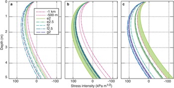
Vertical compression above the neutral axis increases on the falling tide near the fixed end of the domain, when the curvature is convex up close to the grounding line and concave up farther downstream. The opposite holds on the rising tide. This detail of the bending is important. As the tide falls (Fig. 11b), stress intensity sweeps higher at stations e2 and e2.5, increasing the likelihood of fracture propagation, while it experiences little change at f2 and sweeps slightly lower at stations f2.5 and g2. Stations e2 and e2.5 are both in the strand crack zone while the others are outside of it. The opposite occurs on the rising tide. Stress intensities in the strand crack zone sweep away from the fracture criterion while sites far downstream of the strand crack zone, f2.5 and g2, sweep toward it. The change in stress intensity is, in both cases, large for sites near the flexure limit boundary and small for sites away from it.