


1. Introduction
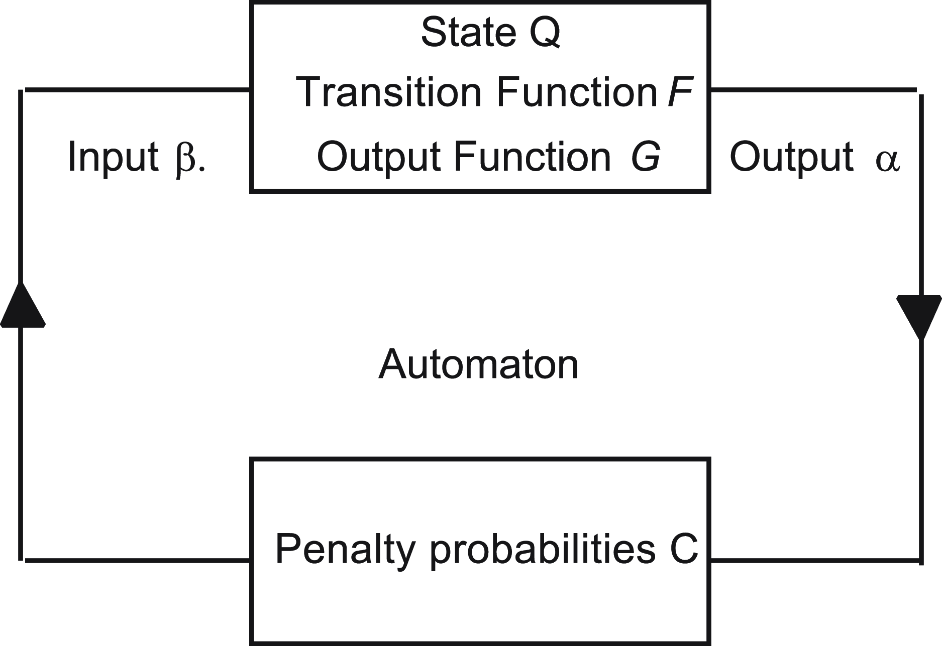
Narendra and Thathachar (Reference Narendra and Thathachar1974) first presented the term Learning Automata (LA) in their 1974 survey. LA consists of an adaptive learning agent interacting with a stochastic environment with incomplete information. Lacking prior knowledge, LA attempts to determine the optimal action to take by first choosing an action randomly and then updating the action probabilities based on the reward/penalty input that the LA receives from the environment. This process is repeated until the optimal action is, finally, achieved. The LA update process can be described by the learning loop shown in Figure 1.
LA interacting with the environment.
The feedback from the LA is a scalar that falls in the interval [0,1]. If the feedback is binary, meaning 0 or 1, then the Environment is called P-type. Whenever the feedback is a discrete values, we call the environment
 $Q-$
type. In the third case where the feedback is any real number in the interval [0,1], we call the environment as
$Q-$
type. In the third case where the feedback is any real number in the interval [0,1], we call the environment as
 $S-$
type.
$S-$
type.
Depending on their Markovian properties, LA can be classified as either ergodic or equipped with characteristics of absorbing barriers. In an ergodic LA system, the final steady state does not depend on the initial state. In contrast, LA with absorbing barriers, the steady state depends on the initial state and when the LA converges, it gets locked into an absorbing state.
Absorbing barrier LA are preferred in static environments, while ergodic LA are suitable for dynamic environments.
LA with artificially absorbing barrier were introduced in the 1980s. In the context of LA, artificial barriers refer to additional constraints or obstacles intentionally imposed on the agent’s learning environment. These barriers can be designed to shape the agent’s behavior, steer its exploration, or promote the discovery of optimal solutions that might not lie in the corners of the simplex.
John Oommen (Reference John Oommen1986), turned a discretized ergodic scheme into an absorbing one by introducing an artificially absorbing barrier that forces the scheme to converge to one of the absorbing barriers. Such a modification led to the advent of new LA families with previously unknown behavior.
In this paper, we devise a LA with artificial barriers for solving a general form of stochastic bimatrix game. Our proposed algorithm addresses bimatrix games which is a more general version of the zero-sum game treated in Lakshmivarahan and Narendra (Reference Lakshmivarahan and Narendra1982).
Reward-
 $\epsilon$
Penalty (
$\epsilon$
Penalty (
 $L_{R-\epsilon P}$
) scheme proposed by Lakshmivarahan and Narendra (Reference Lakshmivarahan and Narendra1982) almost four decades ago, is the only LA scheme that was shown to converge to the optimal mixed Nash equilibrium when no Saddle Point exists in pure strategy, and the proofs were limited to only zero-sum games.
$L_{R-\epsilon P}$
) scheme proposed by Lakshmivarahan and Narendra (Reference Lakshmivarahan and Narendra1982) almost four decades ago, is the only LA scheme that was shown to converge to the optimal mixed Nash equilibrium when no Saddle Point exists in pure strategy, and the proofs were limited to only zero-sum games.
By resorting to the powerful concept of artificial barriers, we propose a LA that converges to an optimal mixed Nash equilibrium even though there may be no Saddle Point when a pure strategy is invoked. Our deployed scheme is of Linear Reward-Inaction (
 $L_{R-I}$
) flavor which is originally an absorbing LA scheme, however, we render it non-absorbing by introducing artificial barriers in an elegant and natural manner, in the sense that the well-known legacy
$L_{R-I}$
) flavor which is originally an absorbing LA scheme, however, we render it non-absorbing by introducing artificial barriers in an elegant and natural manner, in the sense that the well-known legacy
 $L_{R-I}$
scheme can be seen as an instance of our proposed algorithm for a particular choice of the barrier. Furthermore, we present an S-Learning version of our LA with absorbing barriers that is able to handle S-Learning environment in which the feedback is continuous and not binary as in the case of the
$L_{R-I}$
scheme can be seen as an instance of our proposed algorithm for a particular choice of the barrier. Furthermore, we present an S-Learning version of our LA with absorbing barriers that is able to handle S-Learning environment in which the feedback is continuous and not binary as in the case of the
 $L_{R-I}$
. For a generalized analysis of reinforcement learning in game theory, including the
$L_{R-I}$
. For a generalized analysis of reinforcement learning in game theory, including the
 $L_{R-I}$
, we refer the reader to Bloembergen et al. (Reference Bloembergen2015).
$L_{R-I}$
, we refer the reader to Bloembergen et al. (Reference Bloembergen2015).
The contributions of this article can be summarized as follows:
-
We introduce a stochastic game with binary outcomes, specifically a reward or a penalty. We extend our consideration to a game where the probabilities of receiving a reward are determined by the corresponding payoff matrix of each player. Furthermore, we propose a limited information framework, a variant often examined in LA. In this game, each player only observes the outcome of his action, either as a reward or penalty, without knowledge of the other player’s choice. The player might not be even aware that he is playing against an opponent player.
-
We introduce a design principle for our scheme, where players adapt their strategies upon receiving a reward during each round of the repetitive game, yet retain their strategies when faced with a penalty. This approach is in line with the Linear Reward-Inaction,
 ${L_{R - I}}$
paradigm. We further extend our discussion by noting a stark contrast to the paradigm presented by Lakshmivarahan and Narendra (Reference Lakshmivarahan and Narendra1982). In their approach, players consistently revise their strategies every round, with the magnitude of probability adjustments solely based on the receipt of a reward or penalty at each time instance.
${L_{R - I}}$
paradigm. We further extend our discussion by noting a stark contrast to the paradigm presented by Lakshmivarahan and Narendra (Reference Lakshmivarahan and Narendra1982). In their approach, players consistently revise their strategies every round, with the magnitude of probability adjustments solely based on the receipt of a reward or penalty at each time instance. -
Furthermore, we provide an extension of our scheme to handle S-learning environment where the feedback is not binary but rather continuous. The informed reader will notice that our main focus is on the case of P-type environment, while we give enough exposure and attention related to the S-type environment.

2. Related work
Studies on strategic games with LA were focused mainly on traditional
 $L_{R-I}$
which is desirable to use as it can yield Nash equilibrium in pure strategies (Sastry et al., Reference Sastry, Phansalkar and Thathachar1994). Although other ergodic schemes such as
$L_{R-I}$
which is desirable to use as it can yield Nash equilibrium in pure strategies (Sastry et al., Reference Sastry, Phansalkar and Thathachar1994). Although other ergodic schemes such as
 $L_{R-P}$
were used in games (Viswanathan & Narendra, Reference Viswanathan and Narendra1974) with limited information, they did not gain popularity at least when it comes to applications due to their inability to converge to Nash equilibrium. LA has found numerous applications in game theoretical applications such as sensor fusion without knowledge of the ground truth (Yazidi et al., Reference Yazidi2022), for distributed power control in wireless networks and more particularly NOMA (Rauniyar et al., Reference Rauniyar2020), optimization of cooperative tasks (Zhang et al., Reference Zhang, Wang and Gao2020), for content placement in cooperative caching (Yang et al., Reference Yang2020), congestion control in Internet of Things (Gheisari & Tahavori, Reference Gheisari and Tahavori2019), reaching agreement in Ultimatum games utilizing a continuous space strategy rather than working within a discrete actions space (De Jong et al., Reference De Jong, Uyttendaele and Tuyls2008), QoS satisfaction in autonomous mobile edge computing (Apostolopoulos et al., Reference Apostolopoulos, Tsiropoulou and Papavassiliou2018), opportunistic spectrum access (Cao & Cai, Reference Cao and Cai2018) scheduling domestic shiftable loads in smart grids (Thapa et al., Reference Thapa2017), anti-jamming channel selection algorithm for interference mitigation (Jia et al., Reference Jia2017), relay selection in vehicular ad-hoc networks (Tian et al., Reference Tian2017), load balancing by invoking the feedback from a purely local agent (Schaerf et al., Reference Schaerf, Shoham and Tennenholtz1994) etc.
$L_{R-P}$
were used in games (Viswanathan & Narendra, Reference Viswanathan and Narendra1974) with limited information, they did not gain popularity at least when it comes to applications due to their inability to converge to Nash equilibrium. LA has found numerous applications in game theoretical applications such as sensor fusion without knowledge of the ground truth (Yazidi et al., Reference Yazidi2022), for distributed power control in wireless networks and more particularly NOMA (Rauniyar et al., Reference Rauniyar2020), optimization of cooperative tasks (Zhang et al., Reference Zhang, Wang and Gao2020), for content placement in cooperative caching (Yang et al., Reference Yang2020), congestion control in Internet of Things (Gheisari & Tahavori, Reference Gheisari and Tahavori2019), reaching agreement in Ultimatum games utilizing a continuous space strategy rather than working within a discrete actions space (De Jong et al., Reference De Jong, Uyttendaele and Tuyls2008), QoS satisfaction in autonomous mobile edge computing (Apostolopoulos et al., Reference Apostolopoulos, Tsiropoulou and Papavassiliou2018), opportunistic spectrum access (Cao & Cai, Reference Cao and Cai2018) scheduling domestic shiftable loads in smart grids (Thapa et al., Reference Thapa2017), anti-jamming channel selection algorithm for interference mitigation (Jia et al., Reference Jia2017), relay selection in vehicular ad-hoc networks (Tian et al., Reference Tian2017), load balancing by invoking the feedback from a purely local agent (Schaerf et al., Reference Schaerf, Shoham and Tennenholtz1994) etc.
The application of game theory in cybersecurity is also a promising research area attracting lots of attention (Do et al., Reference Do2017; Fielder, Reference Fielder2020; Sokri, Reference Sokri2020). Our LA-based solution is well suited for that purpose. In cybersecurity, algorithms that can converge to mixed equilibria are preferred over those that get locked into pure ones since randomization reduces an attacker’s predictive capability to guess the implemented strategy of the defender. For example, let us consider a repetitive two-person security game comprising of a hacker and network administrator. The hacker intends to disrupt the network by launching a Distributed Denial of Service attack (DDOS) of varying magnitudes that could be classified as high or low. The administrator can use varying levels of security measures to protect the assets. We can assume that the adoption of a strong defense strategy by the defender has an extra cost compared to a low one. Similarly, the usage of a high magnitude attack strategy by the attacker has a higher cost compared to a low magnitude attack strategy. Another example of a security game is the jammer and transmitter game (Vadori et al., Reference Vadori2015) where a jammer is trying to guess the communication channel of the transmitter to interfere and block the communication. The transmitter chooses probabilistically a channel to transmit over and the jammer chooses probabilistically a channel to attack. Clearly converging to pure strategies is neither desirable by the jammer nor by the transmitter as it will give a predictive advantage to the opponent. A pertinent example of an application of our proposed scheme is distributed discrete power control problem (Xing & Chandramouli, Reference Xing and Chandramouli2008). Indeed, in Xing and Chandramouli (Reference Xing and Chandramouli2008), these authors used the counter-part scheme due to Lakshmivarahan and Narendra (Reference Lakshmivarahan and Narendra1982) in order to decide the power level of each terminal in a non-cooperative game setting. The latter authors adopt a utility function due to Saraydar et al. which is expressed as ‘the number of information bits received successfully per Joule of energy expended’ (Saraydar et al., Reference Saraydar, Mandayam and Goodman2002). This utility function depends on a certain number of parameters, such as the interference exercised by the other terminals. More specifically, each terminal is only able to observe local information, namely its utility, without having a knowledge of the power level used by the other terminals. The authors of Xing and Chandramouli (Reference Xing and Chandramouli2008) proved that whenever the power levels of the terminals are discrete, there might be cases where there are multiple Nash equilibria or there may also be mixed ones. However, for continuous power level choices, Saraydar et al. (Reference Saraydar, Mandayam and Goodman2002) have shown that the Nash equilibrium is unique.
3. The game model
In this section, we begin by presenting the formal definition of LA in detail, ensuring a clear understanding of its foundational concepts. Following that, we delve into formalizing the game model that is being investigated.
Formally, a LA is defined by the mean of a quintuple
 $\langle {A,B, Q, F(.,.), G(.)} \rangle$
, where the elements of the quintuple are defined term by term as:
$\langle {A,B, Q, F(.,.), G(.)} \rangle$
, where the elements of the quintuple are defined term by term as:
-
1.
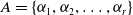
$A=\{ {\alpha}_1, {\alpha}_2, \ldots, {\alpha}_r\}$
gives the set of actions available to the LA, while
${\alpha}(t)$
is the action selected at time instant t by the LA. Note that the LA selects one action at a time, and the selection is sequential. -
2.
$B = \{{\beta}_1, {\beta}_2, \ldots, {\beta}_m\}$
denotes the set of possible input values that the LA can receive.
${\beta}(t)$
denotes the input at time instant t which is a form of feedback. -
3.
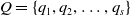
$Q=\{q_1, q_2, \ldots, q_s\}$
represents the states of the LA where Q(t) is the state at time instant t. -
4.
$F(.,.)\,:\, Q \times B \mapsto Q$
is the transition function at time t, such that,
$q(t+1)=F[q(t),{\beta}(t)]$
. In simple terms,
$F(.,.)$
returns the next state of the LA at time instant
$t+1$
given the current state and the input from the environment both at time t using either a deterministic or a stochastic mapping. -
5.
$G(.)$
defines output function, it represents a mapping
$G: Q \mapsto A$
which determines the action of the LA as a function of the state.


The Environment, E is characterized by :
-
$C=\{c_1, c_2, \ldots, c_r\}$
is a set of penalty probabilities, where
$c_i \in C$
corresponds to the penalty of action
${\alpha}_i$
.


Let
 $P(t)= \begin{bmatrix} p_1(t) & p_2(t)\end{bmatrix}^{\intercal}$
denote the mixed strategy of player A at time instant t, where
$P(t)= \begin{bmatrix} p_1(t) & p_2(t)\end{bmatrix}^{\intercal}$
denote the mixed strategy of player A at time instant t, where
 $p_1(t)$
accounts for the probability of adopting strategy 1 and, conversely,
$p_1(t)$
accounts for the probability of adopting strategy 1 and, conversely,
 $p_2(t)$
stands for the probability of adopting strategy 2. Thus, P(t) describes the distribution over the strategies of player A. Similarly, we can define the mixed strategy of player B at time t as
$p_2(t)$
stands for the probability of adopting strategy 2. Thus, P(t) describes the distribution over the strategies of player A. Similarly, we can define the mixed strategy of player B at time t as
 $Q(t)= \begin{bmatrix}q_1(t) & q_2(t)\end{bmatrix}^{\intercal}$
. The extension to more than two actions per player is straightforward following the method analogous to what was used by Papavassilopoulos (Reference Papavassilopoulos1989), which extended the work of Lakshmivarahan and Narendra (Reference Lakshmivarahan and Narendra1982).
$Q(t)= \begin{bmatrix}q_1(t) & q_2(t)\end{bmatrix}^{\intercal}$
. The extension to more than two actions per player is straightforward following the method analogous to what was used by Papavassilopoulos (Reference Papavassilopoulos1989), which extended the work of Lakshmivarahan and Narendra (Reference Lakshmivarahan and Narendra1982).
Let
 $\alpha_A(t) \in \{1,2\}$
be the action chosen by player A at time instant t and
$\alpha_A(t) \in \{1,2\}$
be the action chosen by player A at time instant t and
 $\alpha_B(t) \in \{1,2\}$
be the one chosen by player B, following the probability distributions P(t) and Q(t), respectively. The pair
$\alpha_B(t) \in \{1,2\}$
be the one chosen by player B, following the probability distributions P(t) and Q(t), respectively. The pair
 $(\alpha_A(t),\alpha_B(t)$
) constitutes the joint action at time t, and are pure strategies. Specifically, if
$(\alpha_A(t),\alpha_B(t)$
) constitutes the joint action at time t, and are pure strategies. Specifically, if
 $(\alpha_A(t),\alpha_B(t))=(i,j)$
, the probability of reward for player A is determined by
$(\alpha_A(t),\alpha_B(t))=(i,j)$
, the probability of reward for player A is determined by
 $r_{ij}$
while that of player B is determined by
$r_{ij}$
while that of player B is determined by
 $c_{ij}$
. Player A is in this case the row player while player B is the column player.
$c_{ij}$
. Player A is in this case the row player while player B is the column player.
When we are operating in the P-type mode, the game is defined by two payoff matrices, R and C describing the reward probabilities of player A and player B respectively:
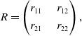 \begin{equation}R=\begin{pmatrix}r_{11} & \quad r_{12} \\[3pt] r_{21} &\quad r_{22}\end{pmatrix},\end{equation}
and the matrix C
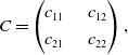 \begin{equation}C=\begin{pmatrix}c_{11} & \quad c_{12} \\[3pt] c_{21} &\quad c_{22}\end{pmatrix},\end{equation}
where, as aforementioned, all the entries of both matrices are probabilities.
In the case where the environment is a S-model type, the latter two matrices are deterministic and describe the feedback as a scalar in the interval [0,1]. For instance, if we operate in the S-type environment, the feedback when both players choose their respective first actions will be the scalar
 $c_{11}$
for player A and not Bernoulli feedback such in the case of P-type environment. It is possible also to consider
$c_{11}$
for player A and not Bernoulli feedback such in the case of P-type environment. It is possible also to consider
 $c_{11}$
as stochastic continuous variable with mean
$c_{11}$
as stochastic continuous variable with mean
 $c_{11}$
and which realization in
$c_{11}$
and which realization in
 $c_{11}$
, however, for the sake of simplicity we consider
$c_{11}$
, however, for the sake of simplicity we consider
 $c_{11}$
, and consequently C and R as deterministic. The asymptotic convergence proofs for the
$c_{11}$
, and consequently C and R as deterministic. The asymptotic convergence proofs for the
 $S-$
type environment will remain valid independently of whether C and R are deterministic or whether they are obtained from a distribution with support in the interval [0,1] and with their means defined by the matrices.
$S-$
type environment will remain valid independently of whether C and R are deterministic or whether they are obtained from a distribution with support in the interval [0,1] and with their means defined by the matrices.
Independently of the environment type, whether it is
 $P-$
type or
$P-$
type or
 $S-$
type environments, we have three cases to be distinguished for equilibria:
$S-$
type environments, we have three cases to be distinguished for equilibria:
-
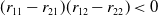
Case 1: if
$(r_{11}-r_{21})(r_{12}-r_{22})<0$
,
$(c_{11}-c_{12})(c_{21}-c_{22})<0$
and
$(r_{11}-r_{21})(c_{11}-c_{12})<0$
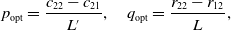
, there is just one mixed equilibrium. The first case depicts the situation where no Saddle Point exists in pure strategies. In other words, the only Nash equilibrium is a mixed one. Based on the fundamentals of Game Theory, the optimal mixed strategies can be shown to be the following:where
\begin{align*}p_{\rm opt}= \frac{c_{22}-c_{21}}{L^{\prime}}, \quad q_{\rm opt}=\frac{r_{22}-r_{12}}{L},\end{align*}
$L=(r_{11}+r_{22})-(r_{12}+r_{21})$
and
$L^{\prime}=(c_{11}+c_{22})-(c_{12}+c_{21})$
.
-
Case 2: if
$(r_{11}-r_{21})(r_{12}-r_{22})>0$
or
$(c_{11}-c_{12})(c_{21}-c_{22})>0$
, then there is just one pure equilibrium since there is one player at least who has a dominant strategy. -
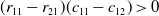
Case 3: if
$(r_{11}-r_{21})(r_{12}-r_{22})<0$
,
$(c_{11}-c_{12})(c_{21}-c_{22})<0$
and
$(r_{11}-r_{21})(c_{11}-c_{12})>0$
, there are two pure equilibria and one mixed equilibrium.


In strategic games, Nash equilibria are equivalently called the ‘Saddle Points’ for the game. Since the outcome for a given joint action is stochastic, the game is of stochastic genre.
4. Game theoretical LA algorithm based on the
$L_{R-I}$
with artificial barriers

In this section, we shall present our
 $L_{R-I}$
with artificial barriers that is devised specially for the P-type environments.
$L_{R-I}$
with artificial barriers that is devised specially for the P-type environments.
4.1. Non-absorbing artificial barriers
As we have seen above from surveying the literature, an originally ergodic LA can be rendered absorbing by operating a change in its end states. However, what is unknown in the literature is a scheme which is originally absorbing can be rendered ergodic. In many cases, this can be achieved by making the scheme behave according to the absorbing scheme rule over the probability simplex and pushing the probability back inside the simplex whenever the scheme approaches absorbing barriers. Such a scheme is novel in the field of LA and its advantage is that the strategies avoid being absorbed in non-desirable absorbing barriers. Further, and interestingly, by countering the absorbing barriers, the scheme can migrate stochastically towards a desirable mixed strategy. Interestingly, as we will see later in the paper, even if the optimal strategy corresponds to an absorbing barrier the scheme will approach it. Thus, the scheme converges to mixed strategies whenever they correspond to optimal strategies while approaching the absorbing states whenever they are the optimal strategies. We shall give the details of our devised scheme in the next section which enjoys the above mentioned properties.
4.2. Non-absorbing Gagme playing
At this juncture, we shall present the design of our proposed LA scheme together with some theoretical results demonstrating that it can converge to the Saddle Points of the game even if the Saddle Point is a mixed Nash equilibrium. Our solution presents a new variant of the
 $L_{R-I}$
scheme, which is made rather ergodic by modifying the update rule in a general form which makes the original
$L_{R-I}$
scheme, which is made rather ergodic by modifying the update rule in a general form which makes the original
 $L_{R-I}$
with absorbing barriers corresponding to the corners of the simplex an instance of the latter general scheme for a particular choice of parameters of the scheme. The proof of convergence is based on Norman’s theory for learning processes characterized by small learning steps (Norman, Reference Norman1972; Narendra & Thathachar, Reference Narendra and Thathachar2012).
$L_{R-I}$
with absorbing barriers corresponding to the corners of the simplex an instance of the latter general scheme for a particular choice of parameters of the scheme. The proof of convergence is based on Norman’s theory for learning processes characterized by small learning steps (Norman, Reference Norman1972; Narendra & Thathachar, Reference Narendra and Thathachar2012).
We introduce
 $p_{max}$
as the artificial barrier which is a real value close to 1. Similarly, we introduce
$p_{max}$
as the artificial barrier which is a real value close to 1. Similarly, we introduce
 $p_{min}=1-p_{max}$
which corresponds to the lowest value any action probability can take. In order to enforce the constraint that the probability of any action for both players remains within the interval
$p_{min}=1-p_{max}$
which corresponds to the lowest value any action probability can take. In order to enforce the constraint that the probability of any action for both players remains within the interval
 ${ [}p_{min}, p_{max} {]}$
one should start by choosing initial values of
${ [}p_{min}, p_{max} {]}$
one should start by choosing initial values of
 $p_1(0)$
and
$p_1(0)$
and
 $q_1(0)$
in the same interval, and further resorting to updates rules that ensure that each update keeps the probabilities within the same interval.
$q_1(0)$
in the same interval, and further resorting to updates rules that ensure that each update keeps the probabilities within the same interval.
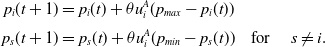
If the outcome from the environment is a reward at a time t for action
 $i \in \{1,2\}$
, the update rule is given by:
$i \in \{1,2\}$
, the update rule is given by:
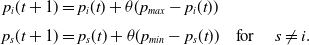 \begin{equation}\begin{aligned}p_i(t+1) & = p_i(t)+\theta (p_{max}-p_i(t))\\[3pt]p_s(t+1) & = p_s(t)+\theta (p_{min}-p_s(t)) &\textrm{for } \quad s\ne i.\end{aligned}\end{equation}
where
 $\theta$
is a learning parameter. The informed reader observes that the update rules coincide with the classical
$\theta$
is a learning parameter. The informed reader observes that the update rules coincide with the classical
 $L_{R-I}$
except that
$L_{R-I}$
except that
 $p_{max}$
replaces unity for updating
$p_{max}$
replaces unity for updating
 $p_i(t+1)$
and that
$p_i(t+1)$
and that
 $p_{min}$
replaces zero for updating
$p_{min}$
replaces zero for updating
 $p_s(t+1)$
.
$p_s(t+1)$
.
Following the Inaction principle of the
 $L_{R-I}$
, whenever the player receives a penalty, its action probabilities are kept unchanged which is formally given by:
$L_{R-I}$
, whenever the player receives a penalty, its action probabilities are kept unchanged which is formally given by:
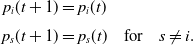 \begin{equation}\begin{aligned}p_i(t+1) & = p_i(t)\\[3pt]p_s(t+1) & = p_s(t) &\textrm{for} \quad s\ne i.\end{aligned}\end{equation}
The update rules for the mixed strategy
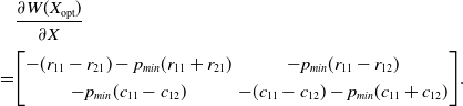
 $q(t+1)$
are defined in a similar fashion. We shall now move to a theoretical analysis of the convergence properties of our proposed algorithm for solving a strategic game. In order to denote the optimal Nash equilibrium of the game we use the pair
$q(t+1)$
are defined in a similar fashion. We shall now move to a theoretical analysis of the convergence properties of our proposed algorithm for solving a strategic game. In order to denote the optimal Nash equilibrium of the game we use the pair
 $(p_{\mathrm{opt}},q_{\mathrm{opt}})$
.
$(p_{\mathrm{opt}},q_{\mathrm{opt}})$
.
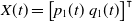
Let the vector
 $X(t) = \begin{bmatrix} p_1(t) & q_1(t) \end{bmatrix}^{\intercal}$
. We resort to the notation
$X(t) = \begin{bmatrix} p_1(t) & q_1(t) \end{bmatrix}^{\intercal}$
. We resort to the notation
 $\Delta X(t) = X(t+1) - X(t)$
. For denoting the conditional expected value operator we use the nomenclature
$\Delta X(t) = X(t+1) - X(t)$
. For denoting the conditional expected value operator we use the nomenclature
 $\mathbb{E}[{\cdot} | {\cdot}]$
. Using those notations, we introduce the next theorem of the article.
$\mathbb{E}[{\cdot} | {\cdot}]$
. Using those notations, we introduce the next theorem of the article.
Theorem 1. Consider a two-player game with a payoff matrices as in –Equations (3.1) and (3.2), and a learning algorithm defined by Equations (4.1) and (4.2) for both players A and B, with learning rate
 $\theta$
. Then,
$\theta$
. Then,
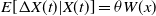 $E[\Delta X(t) | X(t)]=\theta W(x)$
and for every
$E[\Delta X(t) | X(t)]=\theta W(x)$
and for every
 $\epsilon>0$
, there exists a unique stationary point
$\epsilon>0$
, there exists a unique stationary point
 $X^*=\begin{bmatrix}p_1^* &q_1^*\end{bmatrix}^{\intercal}$
satisfying:
$X^*=\begin{bmatrix}p_1^* &q_1^*\end{bmatrix}^{\intercal}$
satisfying:
-
1.
$W(X^*)=0$
; -
2.
$|X^*-X_{\rm opt}|<\epsilon$
.


Proof We start by first computing the conditional expected value of the increment
 $\Delta X(t)$
:
$\Delta X(t)$
:
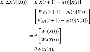 \begin{align*}E[\Delta X(t) | X(t)]&= E[X(t+1)-X(t)\vert X(t)]\\[3pt]&=\begin{bmatrix}E[p_1(t+1)-p_1(t)\vert X(t)] \\[5pt] E[q_1(t+1)-q_1(t)\vert X(t)])\end{bmatrix}\\[5pt]&=\theta\begin{bmatrix}W_1(X(t)) \\[5pt] W_2(X(t))\end{bmatrix}\\[3pt]&=\theta W(X(t)),\end{align*}
where the above format is possible since all possible updates share the form
 $\Delta X(t) = \theta W(t)$
, for some W(t), as given in Equation (4.1). For ease of notation, we drop the dependence on t with the implicit assumption that all occurrences of X,
$\Delta X(t) = \theta W(t)$
, for some W(t), as given in Equation (4.1). For ease of notation, we drop the dependence on t with the implicit assumption that all occurrences of X,
 $p_1$
and
$p_1$
and
 $q_1$
represent X(t),
$q_1$
represent X(t),
 $p_1(t)$
and
$p_1(t)$
and
 $q_1(t)$
respectively.
$q_1(t)$
respectively.
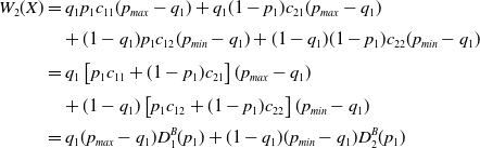
 $W_1(x)$
is then:
$W_1(x)$
is then:
 \begin{align}W_1({X}) & = p_1 q_1 r_{11} (p_{max} - p_1) + p_1 (1-q_1) r_{12} (p_{max} - p_1)\nonumber\\[3pt] & \quad + (1-p_1) q_1 r_{21} (p_{min} - p_1) \nonumber\\[3pt] & \quad + (1-p_1) (1-q_1) r_{22} (p_{min} - p_1) \nonumber\\[3pt] & = p_1 \left [ q_1 r_{11} + (1-q_1) r_{12} \right ] (p_{max} - p_1)\\[3pt] & \quad + (1-p_1) \left [ q_1 r_{21} + (1-q_1) r_{22} \right ] (p_{min} - p_1)\nonumber \\[3pt] & = p_1 (p_{max} - p_1) D_1^A(q_1) + (1-p_1) (p_{min} - p_1) D_2^A(q_1),\nonumber \end{align}
where,
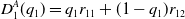 \begin{equation}D_{1}^{A}(q_1)=q_1 r_{11}+(1-q_1)r_{12}\end{equation}
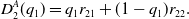 \begin{equation}D_{2}^{A}(q_1)=q_1 r_{21}+(1-q_1)r_{22}.\end{equation}
By replacing
 $p_{max} = 1-p_{min}$
and rearranging the expression we get:
$p_{max} = 1-p_{min}$
and rearranging the expression we get:
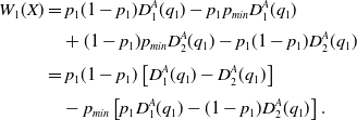 \begin{align*}W_{1}({X})& = p_1(1-p_1)D_1^A(q_1) - p_1 p_{min} D_1^A(q_1) \\[3pt]& \quad + (1-p_1)p_{min} D_2^A(q_1) - p_1(1-p_1)D_2^A(q_1) \\[3pt]& = p_1 (1-p_1) \left [ D_{1}^{A}(q_1)-D_{2}^{A}(q_1)\right ] \\[3pt]& \quad -p_{min} \left [ p_1 D_{1}^{A}(q_1)-(1-p_1) D_{2}^{A}(q_1)\right ].\end{align*}
Similarly, we can get
 \begin{align} W_2({X}) & = q_1 p_1 c_{11} (p_{max} - q_1) + q_1 (1-p_1) c_{21} (p_{max} - q_1)\nonumber\\[3pt] & \quad + (1-q_1) p_1 c_{12} (p_{min} - q_1) + (1-q_1) (1-p_1) c_{22} (p_{min} - q_1) \\[3pt] & = q_1 \left [ p_1 c_{11} + (1-p_1) c_{21} \right ] (p_{max} - q_1) \nonumber\\[3pt] & \quad + (1-q_1) \left [ p_1 c_{12} + (1-p_1) c_{22} \right ] (p_{min} - q_1) \nonumber\\[3pt] & = q_1 (p_{max} - q_1) D_1^B(p_1) + (1-q_1) (p_{min} - q_1) D_2^B(p_1)\nonumber \end{align}
where
 \begin{equation}D_{1}^{B}(p_1)=p_1 c_{11}+(1-p_1)c_{21}\end{equation}
 \begin{equation}D_{2}^{B}(p_1)=p_1 c_{12}+(1-p_1)c_{22}.\end{equation}
By replacing
 $p_{max} = 1-p_{min}$
and rearranging the expression we get:
$p_{max} = 1-p_{min}$
and rearranging the expression we get:
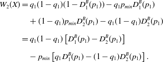 \begin{align}W_{2}({X})& = q_1(1-q_1)(1-D_1^B(p_1)) - q_1 p_{min} D_1^B(p_1) \nonumber\\[6pt]& \quad + (1-q_1)p_{min} D_2^B(p_1) - q_1(1-q_1) D_2^B(p_1) \nonumber\\[6pt]& = q_1 (1-q_1) \left [ D_{1}^{B}(p_1)-D_{2}^{B}(p_1)\right ]\\[6pt]&\quad - p_{min} \left [ q_1 D_{1}^{B}(p_1)-(1-q_1)D_{2}^{B}(p_1)\right ].\nonumber\end{align}
We need to address the three identified cases.
Consider Case 1: Only One Mixed Equilibrium Case, where there is only a single mixed equilibrium. We get
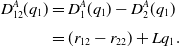 \begin{equation}\begin{aligned}D^{A}_{12}(q_1)&=D_{1}^{A}(q_1)-D_{2}^{A}(q_1)\\[3pt]&=(r_{12}-r_{22})+L q_1.\end{aligned}\end{equation}
We also should distinguish details of the equilibrium according to the entries in the payoff matrices R and C for Case 1. This case can be divided into two sub-cases. The first sub-case is given by:
 \begin{equation} r_{11} > r_{21}, r_{12} < r_{22};\, c_{11} < c_{12}, c_{21} > c_{22},\end{equation}
The second sub-case is given by:
 \begin{equation} r_{11} < r_{21}, r_{12} > r_{22};\, c_{11} > c_{12}, c_{21} < c_{22}, \end{equation}
For the sake of brevity, we consider the first sub-case given by condition Equation 4.11. We have
 $L>0$
, since
$L>0$
, since
 $r_{11} > r_{12}$
and
$r_{11} > r_{12}$
and
 $r_{22} > r_{21}$
. Therefore
$r_{22} > r_{21}$
. Therefore
 $D_{12}^{A}(q_1)$
is an increasing function of
$D_{12}^{A}(q_1)$
is an increasing function of
 $q_1$
and
$q_1$
and
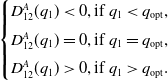 \begin{equation}\begin{cases}D_{12}^{A}(q_1) <0, \hbox{if } q_1< q_{\rm opt},\\[3pt]D_{12}^{A}(q_1) =0, \hbox{if } q_1=q_{\rm opt},\\[3pt]D_{12}^{A}(q_1) > 0, \hbox{if } q_1>q_{\rm opt}.\end{cases}\end{equation}
For a given
 $q_1$
,
$q_1$
,
 $W_1({X})$
is quadratic in
$W_1({X})$
is quadratic in
 $p_1$
. Also, we have:
$p_1$
. Also, we have:
 \begin{equation} \begin{aligned} W_1 \left (\begin{bmatrix} 0\\[3pt] q_1 \end{bmatrix}\right ) & = p_{min} D_{2}^{A}(q_1) > 0 \\[3pt] W_1 \left (\begin{bmatrix} 1\\[3pt] q_1 \end{bmatrix}\right ) & = -p_{min} D_{1}^{A}(q_1) < 0. \end{aligned}\end{equation}
Since
 $W_1({X})$
is quadratic with a negative second derivative with respect to
$W_1({X})$
is quadratic with a negative second derivative with respect to
 $p_1$
, and since the inequalities in Equation (4.14) are strict, it admits a single root
$p_1$
, and since the inequalities in Equation (4.14) are strict, it admits a single root
 $p_1$
for
$p_1$
for
 $p_1 \in [0,1]$
. Moreover, we have
$p_1 \in [0,1]$
. Moreover, we have
 $W_1({X}) = 0$
for some
$W_1({X}) = 0$
for some
 $p_1$
such that:
$p_1$
such that:
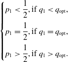 \begin{equation} \begin{cases}p_1 <\dfrac{1}{2}, \hbox{if } q_1< q_{\rm opt},\\[9pt]p_1 =\dfrac{1}{2}, \hbox{if } q_1=q_{\rm opt},\\[9pt]p_1 >\dfrac{1}{2}, \hbox{if } q_1>q_{\rm opt}.\end{cases}\end{equation}
Using a similar argument, we can see that there exists a single solution for each
 $p_1$
, and as
$p_1$
, and as
 $p_{min} \to 0$
, we conclude that
$p_{min} \to 0$
, we conclude that
 $W_{1}(X)=0$
whenever
$W_{1}(X)=0$
whenever
 $p_1 \in \{0, p_{\mathrm{opt}}, 1\}$
. Arguing in a similar manner we see that
$p_1 \in \{0, p_{\mathrm{opt}}, 1\}$
. Arguing in a similar manner we see that
 $W_2(X)=0$
when:
$W_2(X)=0$
when:
 $X \in \left\{\begin{bmatrix} 0 \\[3pt] 0 \end{bmatrix},\begin{bmatrix} 0 \\[3pt] 1 \end{bmatrix}, \begin{bmatrix} 1 \\[3pt] 0 \end{bmatrix},\begin{bmatrix} 1 \\[3pt] 1 \end{bmatrix},\begin{bmatrix} p_{\mathrm{opt}} \\[3pt] q_{\mathrm{opt}} \end{bmatrix}\right\} $
.
$X \in \left\{\begin{bmatrix} 0 \\[3pt] 0 \end{bmatrix},\begin{bmatrix} 0 \\[3pt] 1 \end{bmatrix}, \begin{bmatrix} 1 \\[3pt] 0 \end{bmatrix},\begin{bmatrix} 1 \\[3pt] 1 \end{bmatrix},\begin{bmatrix} p_{\mathrm{opt}} \\[3pt] q_{\mathrm{opt}} \end{bmatrix}\right\} $
.
Thus, there exists a small enough value for
 $p_{min}$
such that
$p_{min}$
such that
 $X^*=[p^*,q^*]^{\intercal}$
satisfies
$X^*=[p^*,q^*]^{\intercal}$
satisfies
 $W_2(X^*)=0$
, proving Case 1).
$W_2(X^*)=0$
, proving Case 1).
In the proof of Case 1), we take advantage of the fact that for small enough
 $p_{min}$
, the learning algorithm enters a stationary point, and also identified the corresponding possible values for this point. It is thus always possible to select a small enough
$p_{min}$
, the learning algorithm enters a stationary point, and also identified the corresponding possible values for this point. It is thus always possible to select a small enough
 $p_{min} >0$
such that
$p_{min} >0$
such that
 $X^*$
approaches
$X^*$
approaches
 $X_{\mathrm{opt}}$
, concluding the proof for Case 1).
$X_{\mathrm{opt}}$
, concluding the proof for Case 1).
Case 2) and Case 3) can be derived in a similar manner, and the details are omitted to avoid repetition.
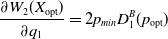
In the next theorem, we show that the expected value of
 $\Delta X(t)$
has a negative definite gradient.
$\Delta X(t)$
has a negative definite gradient.
Theorem 2. The matrix of partial derivatives,
 $\dfrac{\partial W(X^*)}{\partial x}$
is negative definite.
$\dfrac{\partial W(X^*)}{\partial x}$
is negative definite.
Proof. We start the proof by writing the explicit format for
 $\dfrac{\partial W(X)}{\partial X} =\begin{bmatrix} \dfrac{\partial W_{1}(X)}{\partial p_1} & \quad \dfrac{\partial W_{1}(X)}{\partial q_1}\\[12pt]\dfrac{\partial W_{2}(X)}{\partial p_1} &\quad \dfrac{\partial W_{2}(X)}{\partial q_1},\end{bmatrix}$
and then computing each of the entries as below:
$\dfrac{\partial W(X)}{\partial X} =\begin{bmatrix} \dfrac{\partial W_{1}(X)}{\partial p_1} & \quad \dfrac{\partial W_{1}(X)}{\partial q_1}\\[12pt]\dfrac{\partial W_{2}(X)}{\partial p_1} &\quad \dfrac{\partial W_{2}(X)}{\partial q_1},\end{bmatrix}$
and then computing each of the entries as below:
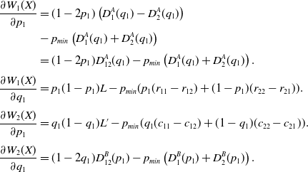 \begin{align*}\frac{\partial W_{1}(X)}{\partial p_1} &= (1-2p_1) \left( D_{1}^{A}(q_1)-D_{2}^{A}(q_1)\right)\\& - p_{min} \left ( D_{1}^{A}(q_1)+ D_{2}^{A}(q_1)\right )\\[3pt]& = (1-2p_1)D^{A}_{12}(q_1) - p_{min} \left ( D_{1}^{A}(q_1)+ D_{2}^{A}(q_1)\right).\\[3pt]\frac{\partial W_{1}(X)}{\partial q_1} & = p_1(1-p_1)L-p_{min}(p_1(r_{11}-r_{12})+ (1-p_1)(r_{22}-r_{21})).\\[3pt]\frac{\partial W_{2}(X)}{\partial p_1} &= q_1(1-q_1) L^{\prime} -p_{min} ( q_1 (c_{11}-c_{12}) + (1-q_1)(c_{22}-c_{21})).\\[3pt]\frac{\partial W_{2}(X)}{\partial q_1} &= (1-2q_1)D^{B}_{12}(p_1) - p_{min} \left ( D_{1}^{B}(p_1)+ D_{2}^{B}(p_1)\right).\end{align*}
As seen in Theorem 1, for a small enough value for
 $p_{min}$
, we can ignore the terms that are weighted by
$p_{min}$
, we can ignore the terms that are weighted by
 $p_{min}$
, and we will thus have
$p_{min}$
, and we will thus have
 $\dfrac{\partial W(X^*)}{\partial X} \approx \dfrac{\partial W(X_{\mathrm{opt}})}{\partial X}$
. We now subdivide the analysis into the three cases.
$\dfrac{\partial W(X^*)}{\partial X} \approx \dfrac{\partial W(X_{\mathrm{opt}})}{\partial X}$
. We now subdivide the analysis into the three cases.
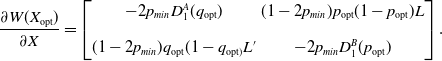
Case 1: No Saddle Point in pure strategies. In this case, we have:
 \begin{equation*}D_{1}^{A}(q_{\rm opt})= D_{2}^{A}(q_{\rm opt}) \quad \text{ and }D_{1}^{B}(p_{\rm opt})= D_{2}^{B}(p_{\rm opt})\end{equation*}
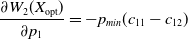
which makes
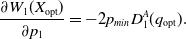 \begin{equation} \frac{\partial W_{1}(X_{\mathrm{opt}})}{\partial p_1} = -2p_{min} D_{1}^{A}(q_{\mathrm{opt}}).\end{equation}
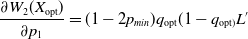
Similarly, we can compute
 \begin{equation} \frac{\partial W_{1}(X_{\mathrm{opt}})}{\partial q_1} = (1-2p_{min})p_{\mathrm{opt}}(1-p_{\mathrm{opt}})L.\end{equation}
The entry
 $\dfrac{\partial W_{2}(X_{\mathrm{opt}})}{\partial p_1}$
can be simplified to:
$\dfrac{\partial W_{2}(X_{\mathrm{opt}})}{\partial p_1}$
can be simplified to:
 \begin{equation}\frac{\partial W_{2}(X_{\mathrm{opt}})}{\partial p_1} = (1-2p_{min})q_{\mathrm{opt}}(1-q_{\mathrm{opt})}L^{\prime}\end{equation}
and
 \begin{equation}\frac{\partial W_{2}(X_{\mathrm{opt}})}{\partial q_1} = 2p_{min}D_1^B(p_{\mathrm{opt}})\end{equation}
resulting in:
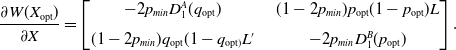 \begin{align} \frac{\partial W(X_{\mathrm{opt}})}{\partial X} = \begin{bmatrix} -2p_{min} D_{1}^{A}(q_{\mathrm{opt}}) & \quad (1-2p_{min})p_{\mathrm{opt}}(1-p_{\mathrm{opt}})L\\[6pt] (1-2p_{min})q_{\mathrm{opt}}(1-q_{\mathrm{opt})}L^{\prime} & \quad -2p_{min}D_1^B(p_{\mathrm{opt}}) \end{bmatrix}.\end{align}
We know that this case can be divided into two sub-cases. Let us consider the first sub-case given by:
 \begin{equation} r_{11} > r_{21}, r_{12} < r_{22};\, c_{11} < c_{12}, c_{21} > c_{22},\end{equation}
Thus,
 $L>0$
and
$L>0$
and
 $L^{\prime}<0$
as a consequence of Equation (4.21)
$L^{\prime}<0$
as a consequence of Equation (4.21)
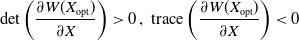
Thus, the matrix given in Equation (4.20) satisfies:
 \begin{equation} \mathrm{det}\left(\frac{\partial W({X}_{\mathrm{opt}})}{\partial x}\right) > 0 \, \text{, } \, \mathrm{trace}\left(\frac{\partial W({X}_{\mathrm{opt}})}{\partial x}\right) < 0,\end{equation}
which implies the
 $2\times 2$
matrix is negative definite.
$2\times 2$
matrix is negative definite.
Case 2: Only one single pure equilibrium. According to this case:
 $(r_{11}-r_{21})(r_{12}-r_{22})>0$
or
$(r_{11}-r_{21})(r_{12}-r_{22})>0$
or
 $(c_{11}-c_{12})(c_{21}-c_{22})>0$
.
$(c_{11}-c_{12})(c_{21}-c_{22})>0$
.
The condition for only one pure equilibrium can be divided into four different sub-cases.
Without loss of generality, we can consider a particular sub-case where
 $q_{\rm opt}=1$
and
$q_{\rm opt}=1$
and
 $p_{\rm opt}=1$
. This reduces to
$p_{\rm opt}=1$
. This reduces to
 $r_{11}-r_{21}>0$
and
$r_{11}-r_{21}>0$
and
 $c_{11}-c_{12}>0$
.
$c_{11}-c_{12}>0$
.
Computing the entries of the matrix for this case yields:
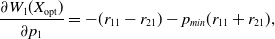 \begin{equation} \frac{\partial W_{1}(X_{\mathrm{opt}})}{\partial p_1} = -(r_{11}-r_{21})-p_{min} (r_{11}+r_{21}),\end{equation}
and
 \begin{equation} \frac{\partial W_{1}(X_{\mathrm{opt}})}{\partial q_1} = -p_{min}(r_{11}-r_{12}).\end{equation}
The entry
 $\dfrac{\partial W_{2}(X_{\mathrm{opt}})}{\partial p_1}$
can be simplified to:
$\dfrac{\partial W_{2}(X_{\mathrm{opt}})}{\partial p_1}$
can be simplified to:
 \begin{equation}\frac{\partial W_{2}(X_{\mathrm{opt}})}{\partial p_1} = -p_{min}(c_{11}-c_{12})\end{equation}
and
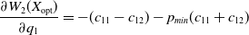 \begin{equation}\frac{\partial W_{2}(X_{\mathrm{opt}})}{\partial q_1} = -(c_{11}-c_{12})-p_{min} (c_{11}+c_{12})\end{equation}
resulting in:
 \begin{align} & \frac{\partial W(X_{\mathrm{opt}})}{\partial X} \\[3pt]\notag = & {\begin{bmatrix} -(r_{11}-r_{21})-p_{min} (r_{11}+r_{21}) & -p_{min}(r_{11}-r_{12})\\[3pt] - p_{min}(c_{11}-c_{12}) & -(c_{11}-c_{12})-p_{min} (c_{11}+c_{12}) \end{bmatrix}}.\end{align}
The matrix in (4.34) satisfies:
 \begin{equation} \mathrm{det}\left(\frac{\partial W(X_{\mathrm{opt}})}{\partial X}\right) > 0 \, \text{, } \, \mathrm{trace}\left(\frac{\partial W(X_{\mathrm{opt}})}{\partial X}\right) < 0\end{equation}
for a sufficiently small value of
 $p_{min}$
, which again implies that the
$p_{min}$
, which again implies that the
 $2\times 2$
matrix is negative definite.
$2\times 2$
matrix is negative definite.
Case 3: Two pure equilibrium and one mixed equilibrium. In this case,
 $(r_{11}-r_{21})(r_{12}-r_{22})<0$
,
$(r_{11}-r_{21})(r_{12}-r_{22})<0$
,
 $(c_{11}-c_{12})(c_{21}-c_{22})<0$
and
$(c_{11}-c_{12})(c_{21}-c_{22})<0$
and
 $(r_{11}-r_{21})(c_{11}-c_{12})>0$
.
$(r_{11}-r_{21})(c_{11}-c_{12})>0$
.
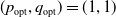
Without loss of generality, we suppose that
 $(p_{\rm opt},q_{\rm opt})=(1,1)$
and
$(p_{\rm opt},q_{\rm opt})=(1,1)$
and
 $(p_{\rm opt},q_{\rm opt})=(0,0)$
are the two pure Nash equilibria. This corresponds to a sub-case where:
$(p_{\rm opt},q_{\rm opt})=(0,0)$
are the two pure Nash equilibria. This corresponds to a sub-case where:
 \begin{equation} r_{11}-r_{21}>0, c_{11}-c_{12}>0, r_{22}-r_{12}>0, c_{22}-c_{21}>0, \end{equation}
 $r_{11}-r_{21}>0$
and
$r_{11}-r_{21}>0$
and
 $c_{11}-c_{12}>0$
because of the Nash equilibrium
$c_{11}-c_{12}>0$
because of the Nash equilibrium
 $(p_{\rm opt},q_{\rm opt})=(1,1)$
. Similarly,
$(p_{\rm opt},q_{\rm opt})=(1,1)$
. Similarly,
 $r_{22}-r_{12}>0$
and
$r_{22}-r_{12}>0$
and
 $c_{22}-c_{21}>0$
because of the Nash equilibrium
$c_{22}-c_{21}>0$
because of the Nash equilibrium
 $(p_{\rm opt},q_{\rm opt})=(1,1)$
.
$(p_{\rm opt},q_{\rm opt})=(1,1)$
.
Whenever
 $(p_{\rm opt},q_{\rm opt})=(1,1)$
, we obtain stability of the fixed point as demonstrated in the previous case, case 2.
$(p_{\rm opt},q_{\rm opt})=(1,1)$
, we obtain stability of the fixed point as demonstrated in the previous case, case 2.
Now, let us consider the stability for
 $(p_{\rm opt},q_{\rm opt})=(0,0)$
.
$(p_{\rm opt},q_{\rm opt})=(0,0)$
.
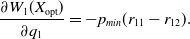
Computing the entries of the matrix for this case yields:
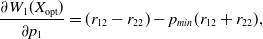 \begin{equation} \frac{\partial W_{1}(X_{\mathrm{opt}})}{\partial p_1} = (r_{12}-r_{22})-p_{min} (r_{12}+r_{22}),\end{equation}
and
 \begin{equation} \frac{\partial W_{1}(X_{\mathrm{opt}})}{\partial q_1} = -p_{min}(r_{22}-r_{21}).\end{equation}
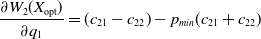
The entry
 $\dfrac{\partial W_{2}(X_{\mathrm{opt}})}{\partial p_1}$
can be simplified to:
$\dfrac{\partial W_{2}(X_{\mathrm{opt}})}{\partial p_1}$
can be simplified to:
 \begin{equation}\frac{\partial W_{2}(X_{\mathrm{opt}})}{\partial p_1} = -p_{min}(c_{22}-c_{12})\end{equation}
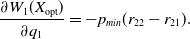
and
 \begin{equation}\frac{\partial W_{2}(X_{\mathrm{opt}})}{\partial q_1} = (c_{21}-c_{22})-p_{min} (c_{21}+c_{22})\end{equation}
resulting in:
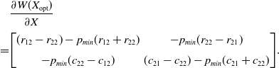 \begin{align} & \frac{\partial W(X_{\mathrm{opt}})}{\partial X} \\[3pt]\notag = & {\begin{bmatrix} (r_{12}-r_{22})-p_{min} (r_{12}+r_{22}) & -p_{min}(r_{22}-r_{21})\\[6pt] -p_{min}(c_{22}-c_{12}) & (c_{21}-c_{22})-p_{min} (c_{21}+c_{22}) \end{bmatrix}}.\end{align}
The matrix in (4.34) satisfies:
 \begin{equation} \mathrm{det}\left(\frac{\partial W(X_{\mathrm{opt}})}{\partial X}\right) > 0 \, \text{, } \, \mathrm{trace}\left(\frac{\partial W(X_{\mathrm{opt}})}{\partial X}\right) < 0\end{equation}
for a sufficiently small value of
 $p_{min}$
, which again implies that the
$p_{min}$
, which again implies that the
 $2\times 2$
matrix is negative definite.
$2\times 2$
matrix is negative definite.
Now, what remains to be shown is that the mixed Nash equilibrium in this case is unstable.
 \begin{align} \frac{\partial W(X_{\mathrm{opt}})}{\partial X} = \begin{bmatrix} -2p_{min} D_{1}^{A}(q_{\mathrm{opt}}) & (1-2p_{min})p_{\mathrm{opt}}(1-p_{\mathrm{opt}})L\\[10pt] (1-2p_{min})q_{\mathrm{opt}}(1-q_{\mathrm{opt})}L^{\prime} & -2p_{min}D_1^B(p_{\mathrm{opt}}) \end{bmatrix}.\end{align}
Using Equation 4.29, we can see that
 $L>0$
and
$L>0$
and
 $L^{\prime}>0$
and thus:
$L^{\prime}>0$
and thus:
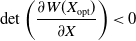 \begin{equation}\mathrm{det}\left(\frac{\partial W(X_{\mathrm{opt}})}{\partial X}\right) < 0\end{equation}
Theorem 3. We consider the update equations given by the
 $L_{R-I}$
scheme. For a sufficiently small
$L_{R-I}$
scheme. For a sufficiently small
 $p_{min}$
approaching 0, and as
$p_{min}$
approaching 0, and as
 $\theta \to 0$
and as time goes to infinity:
$\theta \to 0$
and as time goes to infinity:
 $\begin{bmatrix} E(p_1(t)) & E(q_1(t)) \end{bmatrix}$
 $\rightarrow$
 $\begin{bmatrix}p_{\mathrm{opt}}^* &q_{\mathrm{opt}}^*\end{bmatrix}$
where
 $\begin{bmatrix}p_{\mathrm{opt}}^* &q_{\mathrm{opt}}^*\end{bmatrix}$
corresponds to a Nash equilibrium of the game.
$\begin{bmatrix}p_{\mathrm{opt}}^* &q_{\mathrm{opt}}^*\end{bmatrix}$
corresponds to a Nash equilibrium of the game.
Proof The proof of the result is obtained by virtue of applying a classical result due to Norman (Reference Norman1972), given in the Appendix A, in the interest of completeness.
Norman theorem has been traditionally used to prove considerable amount of the results in the field of LA. In the context of game theoretical LA schemes, Norman theorem has been adapted by Lakshmivarahan and Narendra to derive similar convergence properties of the
 $L_{R-\epsilon P}$
(Lakshmivarahan & Narendra, Reference Lakshmivarahan and Narendra1982) for the zero-sum game. It is straightforward to verify that Assumptions (1)-(6) as required for Norman’s result in the appendix are satisfied.
$L_{R-\epsilon P}$
(Lakshmivarahan & Narendra, Reference Lakshmivarahan and Narendra1982) for the zero-sum game. It is straightforward to verify that Assumptions (1)-(6) as required for Norman’s result in the appendix are satisfied.
Thus, by further invoking Theorem 1 and Theorem 2, the result follows.
Indeed, the convergence proof follows the same line as the proofs in Lakshmivarahan and Narendra (Reference Lakshmivarahan and Narendra1982) and Xing and Chndramouli (2008) which builds upon the Norman theorem.
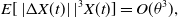
We can write
 \begin{align*}E\{ [\Delta X(t)-X(t)]^{\intercal} [\Delta X(t)-X(t)] | X(t)\}&=\theta^2 s(X(t)),\end{align*}
where
 $s(X(t))=a(X(t))-W(X(t))^{\intercal} W(X(t))$
and
$s(X(t))=a(X(t))-W(X(t))^{\intercal} W(X(t))$
and
 $a(X(t))=E[\Delta X(t)^{\intercal} \Delta X(t)| X(t)]$
.
$a(X(t))=E[\Delta X(t)^{\intercal} \Delta X(t)| X(t)]$
.
The elements of the matrix a(X(t)) can be easily computed. All the states are non-absorbing, it follows that s(X(t)) is positive definite.
Furthermore,
 \begin{align*}E[ \left| \Delta X(t) \right| |^3 X(t)]&=O(\theta^3),\end{align*}
where
 $\left|. \right|$
is the norm function. W(X(t)) has a bounded Lipschitz derivative. In addition, s(X(t)) is Lipschitz.
$\left|. \right|$
is the norm function. W(X(t)) has a bounded Lipschitz derivative. In addition, s(X(t)) is Lipschitz.
It follows that the process X(t) satisfies all conditions of the Norman theorem.
Hence,
 \begin{align}E[\Delta X(t) | X(0)=X]&=\theta y(t \theta)+ O(\theta),\end{align}
where
 \begin{align*}y\prime(t)&=W(y(t))\end{align*}
where
 $y(0)=X(0)=X$
,
$y(0)=X(0)=X$
,
For properties of
 $y\prime(t)$
it follows that Equation (4.38) is uniformly asymptotically stable, that is y(t) converges to
$y\prime(t)$
it follows that Equation (4.38) is uniformly asymptotically stable, that is y(t) converges to
 $X^*$
as
$X^*$
as
 $t \to \infty$
.
$t \to \infty$
.
This implies that
 $\dfrac{X(t)-y(t \theta)}{\sqrt \theta}$
converges in distribution, which implies that E[X(t)] converges.
$\dfrac{X(t)-y(t \theta)}{\sqrt \theta}$
converges in distribution, which implies that E[X(t)] converges.
That is:
 $\lim_{t\to\infty} E[X(t)] $
exists.
$\lim_{t\to\infty} E[X(t)] $
exists.
For small enough
 $p_{min}$
,
$p_{min}$
,
 $X^*$
approximates
$X^*$
approximates
 $X_{\rm opt}$
.
$X_{\rm opt}$
.
It follows that for any
 $\delta>0$
there exits
$\delta>0$
there exits
 $0<\theta^*<1$
, such that
$0<\theta^*<1$
, such that
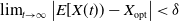 $\lim_{t\to\infty} \left| E[ X(t))-X_{\mathrm{opt}} \right| <\delta$
5. Game theoretical LA algorithm based on the
$S$
-learning with artificial barriers

In this section, we give the update equations for the LA when the environment is of
 $S-$
type.
$S-$
type.
In the case of
 $S-$
type, the game is defined by two payoff matrices, R and C describing a deterministic feedback of player A and player B respectively.
$S-$
type, the game is defined by two payoff matrices, R and C describing a deterministic feedback of player A and player B respectively.
All the entries of both matrices are deterministic numbers like in classical game theory settings.
The environment returns
 $u_i^A(t)$
: the payoff defined by the matrix R for player A at time t whenever player A question chooses an action
$u_i^A(t)$
: the payoff defined by the matrix R for player A at time t whenever player A question chooses an action
 $i \in \{1,2\}$
.
$i \in \{1,2\}$
.
The update rule for the player A that takes into account
 $u_i^A(t)$
is given by:
$u_i^A(t)$
is given by:
 \begin{equation}\begin{aligned}p_i(t+1) & = p_i(t)+\theta u_i^A (p_{max}-p_i(t))\\[3pt]p_s(t+1) & = p_s(t)+\theta u_i^A (p_{min}-p_s(t)) &\textrm{for } \quad s\ne i.\end{aligned}\end{equation}
where
 $\theta$
is a learning parameter.
$\theta$
is a learning parameter.
Note
 $u_i^A$
is the feedback for action i of the player A which is one entry in the
$u_i^A$
is the feedback for action i of the player A which is one entry in the
 $i^th$
row of the matrix R, depending on the action of the player B.
$i^th$
row of the matrix R, depending on the action of the player B.
Similarly we can define
 $u_i^B(t)$
the payoff defined by the matrix C for player B at time t whenever player B question chooses an action
$u_i^B(t)$
the payoff defined by the matrix C for player B at time t whenever player B question chooses an action
 $i \in \{1,2\}$
.
$i \in \{1,2\}$
.
For instance, if at time t, player A takes action 1 and player B takes action 2, then
 $u_1^A(t)=r_{12}$
and
$u_1^A(t)=r_{12}$
and
 $u_2^B(t)=c_{21}$
.
$u_2^B(t)=c_{21}$
.
The update rules for player B can be obtained by analogy to those given for player A.
Theorem 4. We consider the update equations given by the
 $S-$
Learning scheme given above in this Section. For a sufficiently small
$S-$
Learning scheme given above in this Section. For a sufficiently small
 $p_{min}$
approaching 0, and as
$p_{min}$
approaching 0, and as
 $\theta \to 0$
and as time goes to infinity:
$\theta \to 0$
and as time goes to infinity:
 $\begin{bmatrix} E(p_1(t)) & E(q_1(t)) \end{bmatrix}$
 $\rightarrow$
 $\begin{bmatrix}p_{\mathrm{opt}}^* &q_{\mathrm{opt}}^*\end{bmatrix}$
where
 $\begin{bmatrix}p_{\mathrm{opt}}^* &q_{\mathrm{opt}}^*\end{bmatrix}$
corresponds to a Nash equilibrium of the game.
$\begin{bmatrix}p_{\mathrm{opt}}^* &q_{\mathrm{opt}}^*\end{bmatrix}$
corresponds to a Nash equilibrium of the game.
Proof The proofs of this theorem follows the same lines as the proofs given in Section 4 and are omitted here for the sake of brevity.
6. Experimental results
In this Section, we focus on providing thorough experiments for
 $L_{R-I}$
scheme. Some experiments of
$L_{R-I}$
scheme. Some experiments of
 $S-$
LA for handling
$S-$
LA for handling
 $S-$
type environments are given in the Appendix 7 that mainly aim to verify our theoretical findings.
$S-$
type environments are given in the Appendix 7 that mainly aim to verify our theoretical findings.
To verify the theoretical properties of the proposed learning algorithm, we conducted several simulations that will be presented in this section. By using different instances of the payoff matrices R and C, we can experimentally cover the three cases referred to in Section 4.


6.1. Convergence in Case 1
We examine a case of the game where only one mixed Nash equilibrium exists meaning that there is no Saddle Point in pure strategies. The game matrices R and C are given by:
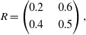 \begin{equation}R=\begin{pmatrix}0.2 & \quad 0.6 \\[3pt] 0.4 & \quad 0.5\end{pmatrix},\end{equation}
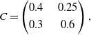 \begin{equation}C=\begin{pmatrix} 0.4 & \quad 0.25 \\[3pt] 0.3 & \quad 0.6\end{pmatrix},\end{equation}
which admits
 $p_{opt}=0.6667$
and
$p_{opt}=0.6667$
and
 $q_{opt}=0.3333$
.
$q_{opt}=0.3333$
.
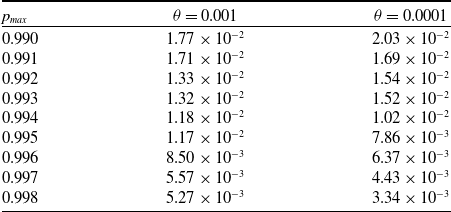
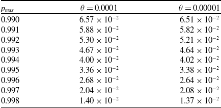
We ran our simulation for
 $5 \times 10^6$
iterations, and present the error in Table 1 for different values of
$5 \times 10^6$
iterations, and present the error in Table 1 for different values of
 $p_{max}$
and
$p_{max}$
and
 $\theta$
as the difference between
$\theta$
as the difference between
 $X_{\mathrm{opt}}$
and the mean over time of X(t) after convergenceFootnote 2. The high value for the number of iterations was chosen in order to eliminate the Monte Carlo error. A significant observation is that the error monotonically decreases as
$X_{\mathrm{opt}}$
and the mean over time of X(t) after convergenceFootnote 2. The high value for the number of iterations was chosen in order to eliminate the Monte Carlo error. A significant observation is that the error monotonically decreases as
 $p_{max}$
goes towards 1 (i.e. when
$p_{max}$
goes towards 1 (i.e. when
 $p_{min} \to 0$
). For instance, for
$p_{min} \to 0$
). For instance, for
 $p_{max}=0.998$
and
$p_{max}=0.998$
and
 $\theta=0.001$
, the proposed scheme yields an error of
$\theta=0.001$
, the proposed scheme yields an error of
 $5.27 \times 10^{-3}$
, and further reducing
$5.27 \times 10^{-3}$
, and further reducing
 $\theta=0.0001$
leads to an error of
$\theta=0.0001$
leads to an error of
 $3.34 \times 10^{-3}$
.
$3.34 \times 10^{-3}$
.
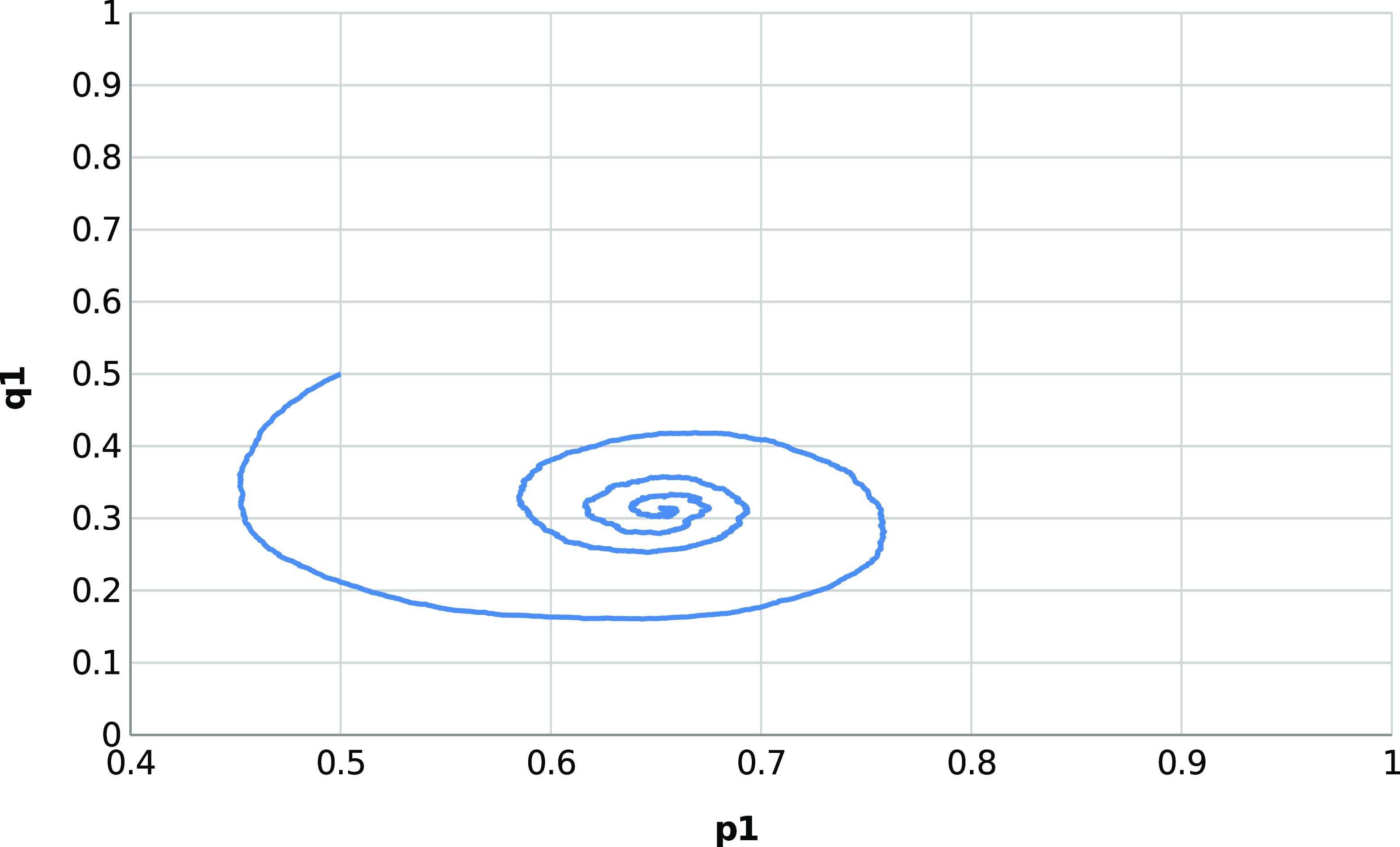
The behavior scheme is illustrated in Figure 2 showing the trajectory of the mixed strategies for both players (given by X(t)) for an ensemble of 1000 runs using
 $\theta=0.01$
and
$\theta=0.01$
and
 $p_{max}=0.99$
.
$p_{max}=0.99$
.


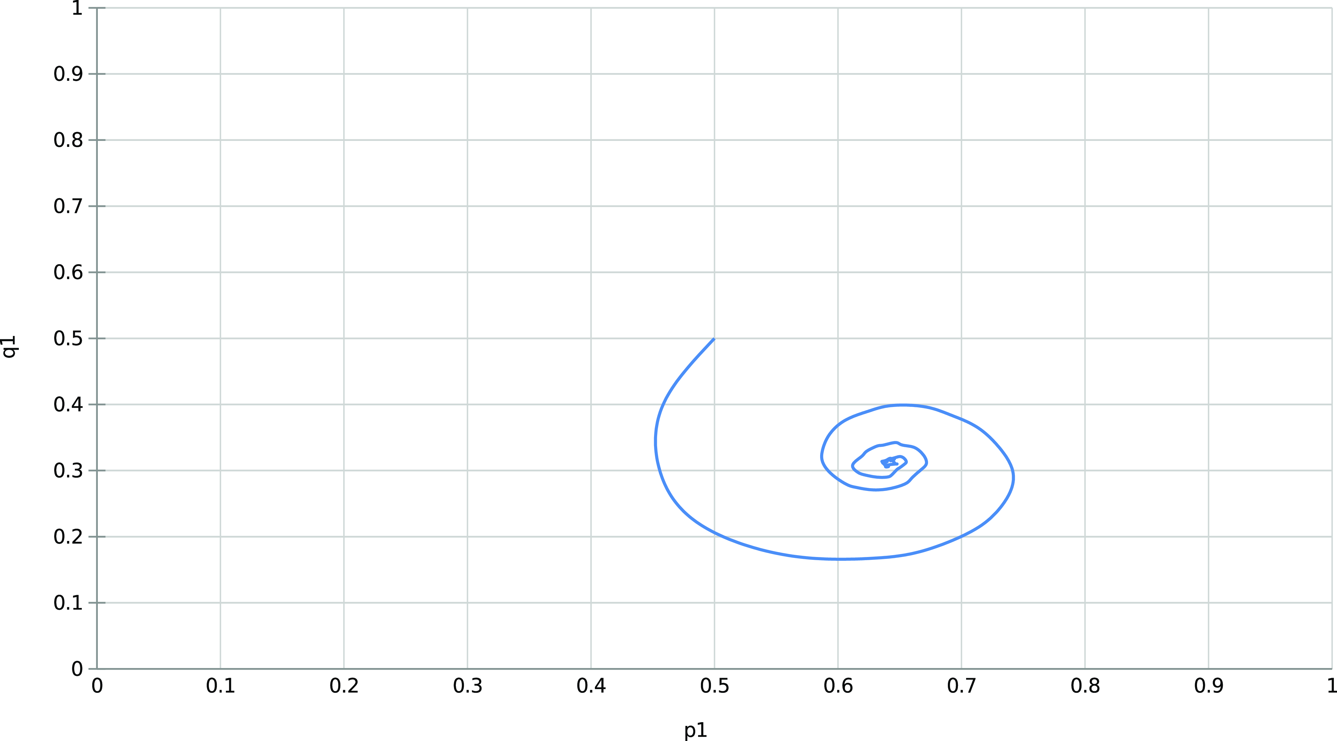
The trajectory of the ensemble enables us to notice the mean evolution of the mixed strategies. The spiral pattern results from one of the players adjusting to the strategy used by the other before the former learns by readjusting its strategy. The process is repeated, thus leading to more minor corrections until the players reach the Nash equilibrium.
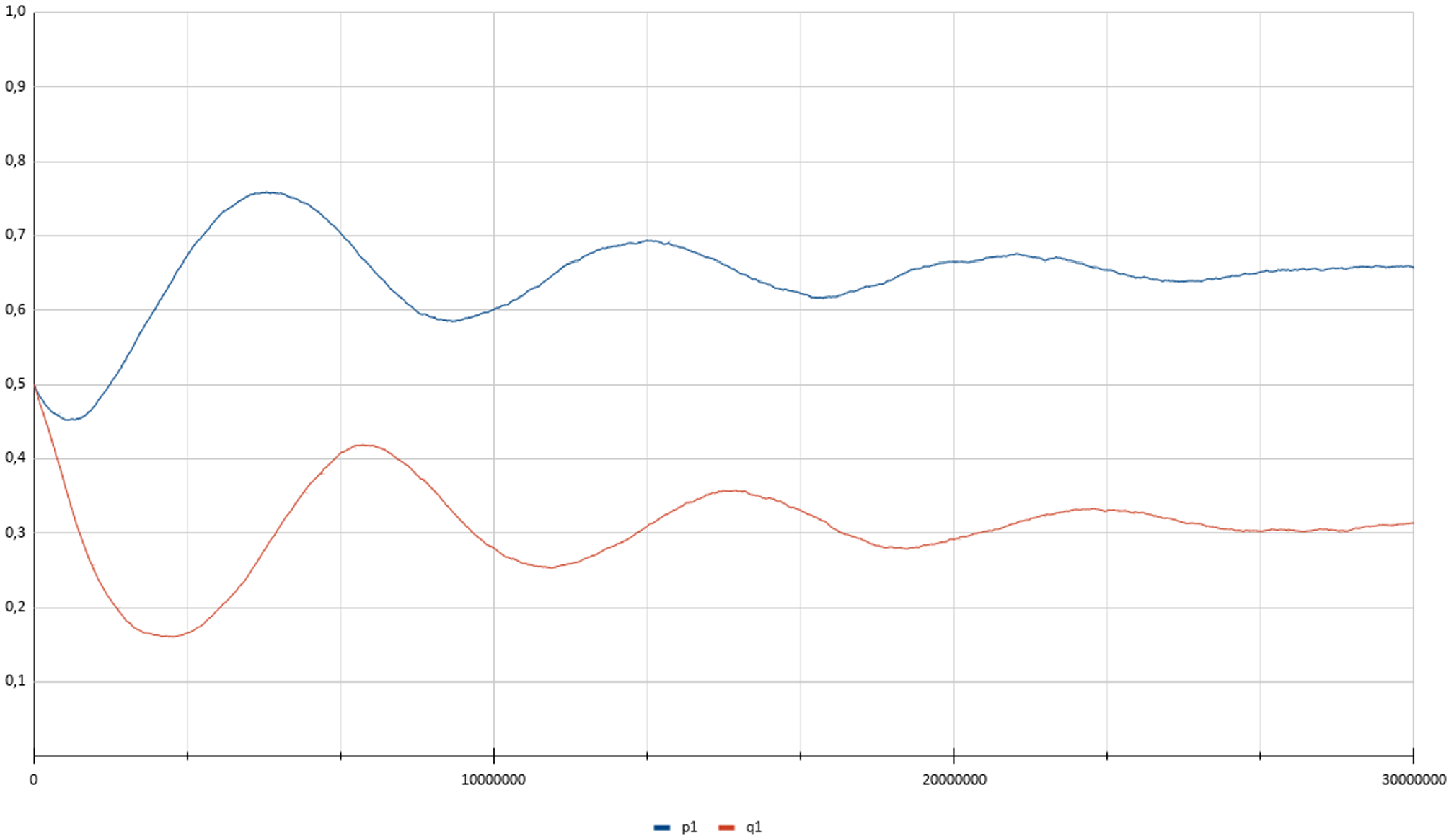
The process can be visualized in Figure 3 presenting the time evolution of the strategies of both players for a single experiment with
 $p_{max}=0.99$
and
$p_{max}=0.99$
and
 $\theta=0.00001$
over
$\theta=0.00001$
over
 $3\times10^7$
steps. We observe an oscillatory behavior which vanishes as the players play for more iterations. It is worth noting that a larger value of
$3\times10^7$
steps. We observe an oscillatory behavior which vanishes as the players play for more iterations. It is worth noting that a larger value of
 $\theta$
will cause more steady state error (as specified in Theorem 1), but it will also disrupt this behavior as the players take larger updates whenever they receive a reward. Furthermore, decreasing
$\theta$
will cause more steady state error (as specified in Theorem 1), but it will also disrupt this behavior as the players take larger updates whenever they receive a reward. Furthermore, decreasing
 $\theta$
results in a smaller convergence error, but also affects negatively the convergence speed as more iterations are required to achieve convergence. Figure 4 depicts the trajectories of the probabilities
$\theta$
results in a smaller convergence error, but also affects negatively the convergence speed as more iterations are required to achieve convergence. Figure 4 depicts the trajectories of the probabilities
 $p_1$
and
$p_1$
and
 $q_1$
for the same settings as those in Figure 3.
$q_1$
for the same settings as those in Figure 3.


Trajectory of X(t) where
 $p_{opt}=0.6667$
and
$p_{opt}=0.6667$
and
 $q_{opt}=0.3333$
, using
$q_{opt}=0.3333$
, using
 $p_{max}=0.99$
and
$p_{max}=0.99$
and
 $\theta=0.00001$
.
$\theta=0.00001$
.
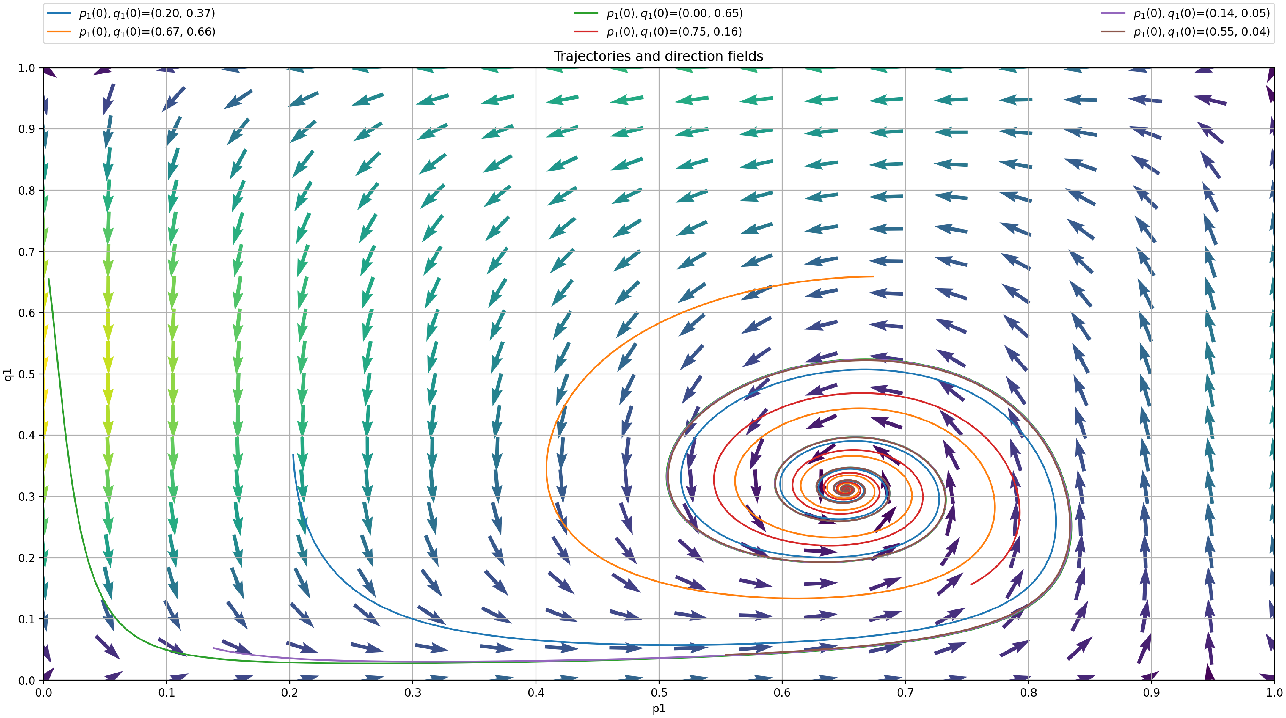
Now, we turn our attention to the analysis of the deterministic Ordinary Differential Equation (ODE) corresponding to our LA with barriers and plot it in Figure 5. The trajectory of the ODE is conform with our intuition and the results of the LA run in Figure 4. The two ODE are given by:
 \begin{align} \frac{dp_1}{dt}= W_1({X}) = p_1 (p_{max} - p_1) D_1^A(q_1) + (1-p_1) (p_{min} - p_1) D_2^A(q_1), \end{align}
and,
 \begin{align} \frac{dq_1}{dt}= W_1({X}) = p_1 (p_{max} - p_1) D_1^A(q_1) + (1-p_1) (p_{min} - p_1) D_2^A(q_1), \end{align}
To obtain the ODE for a particular example, we need just to replace the entries of R and C in the ODE by their values. In this sense to plot the ODE trajectories we only need to know R and C and of course
 $p_{max}$
.
$p_{max}$
.
6.2. Case 2: One pure equilibrium
At this juncture, we shall experimentally show that the scheme possess still plausible convergence properties even in case where there is a single saddle point in pure strategies and that our proposed LA will approach the optimal pure equilibria. For this sake, we consider a case of the game where there is a single pure equilibrium which falls in the category of Case 2 with
 $p_{opt}=1$
and
$p_{opt}=1$
and
 $q_{opt}=0$
. The payoff matrices R and C for the games are given by:
$q_{opt}=0$
. The payoff matrices R and C for the games are given by:
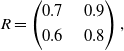 \begin{equation}R=\begin{pmatrix}0.7 & \quad 0.9 \\[3pt] 0.6 & \quad 0.8\end{pmatrix},\end{equation}
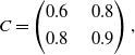 \begin{equation}C=\begin{pmatrix} 0.6 & \quad 0.8 \\[3pt] 0.8 & \quad 0.9 \end{pmatrix},\end{equation}
We first show the convergence errors of our method in Table 2. As in the previous simulation for Case 1, the errors are on the order to
 $10^{-2}$
for larger values of
$10^{-2}$
for larger values of
 $p_{max}$
. We also observe that steady state error is slightly higher compared to the previous case of mixed Nash described by Equations (6.1) and (6.2) which is treated in the previous section.
$p_{max}$
. We also observe that steady state error is slightly higher compared to the previous case of mixed Nash described by Equations (6.1) and (6.2) which is treated in the previous section.


Trajectory of ODE using
 $p_{max}=0.99$
for case 1.
$p_{max}=0.99$
for case 1.
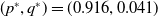
We then plot the ODE for
 $p_{max}=0.99$
as shown in Figure 6. According to the ODE in Figure 6, we are expecting that the LA will converge towards the attractor of the ODE which corresponds to
$p_{max}=0.99$
as shown in Figure 6. According to the ODE in Figure 6, we are expecting that the LA will converge towards the attractor of the ODE which corresponds to
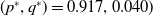 $(p^*,q^*)=0.917, 0.040)$
as
$(p^*,q^*)=0.917, 0.040)$
as
 $\theta$
goes to zero. We see that
$\theta$
goes to zero. We see that
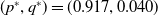 $(p^*,q^*)=(0.917, 0.040)$
approaches
$(p^*,q^*)=(0.917, 0.040)$
approaches
 $(p_{opt},q_{opt})=(1, 0)$
but there is still a gap between them. This is also illustrated in Figure 7 where we also consistently observe that the LA converges towards
$(p_{opt},q_{opt})=(1, 0)$
but there is still a gap between them. This is also illustrated in Figure 7 where we also consistently observe that the LA converges towards
 $(p^*,q^*)=(0.916, 0.041)$
after running our LA for 30 000 iterations with an ensemble of 1000 experiments. The main limitation of introducing artificial barriers whenever the optimal equilibrium is pure is choosing
$(p^*,q^*)=(0.916, 0.041)$
after running our LA for 30 000 iterations with an ensemble of 1000 experiments. The main limitation of introducing artificial barriers whenever the optimal equilibrium is pure is choosing
 $p_{max}$
even slightly away from 1 (such as
$p_{max}$
even slightly away from 1 (such as
 $0.99$
), gives a large deviation in the convergence
$0.99$
), gives a large deviation in the convergence
 $(p^*, q^*) = (0.916, 0.041)$
which is somehow far from the optimal value
$(p^*, q^*) = (0.916, 0.041)$
which is somehow far from the optimal value
 $(p_{opt},q_{opt})=(1, 0)$
. It appears as if, in the case of pure equilibrium, for slightly large
$(p_{opt},q_{opt})=(1, 0)$
. It appears as if, in the case of pure equilibrium, for slightly large
 $p_{min}$
, we can get a large deviation from
$p_{min}$
, we can get a large deviation from
 $(p_{opt},q_{opt})$
. In order to mitigate this issue, one can introduce an extra mechanism that would detect that convergence should take place into the corners of the simplex, implying a pure Nash equilibrium, and reducing
$(p_{opt},q_{opt})$
. In order to mitigate this issue, one can introduce an extra mechanism that would detect that convergence should take place into the corners of the simplex, implying a pure Nash equilibrium, and reducing
 $p_{min}$
over time to ensure such convergence.
$p_{min}$
over time to ensure such convergence.
Trajectory of the deterministic ODE using
 $p_{max}=0.99$
for case 2.
$p_{max}=0.99$
for case 2.
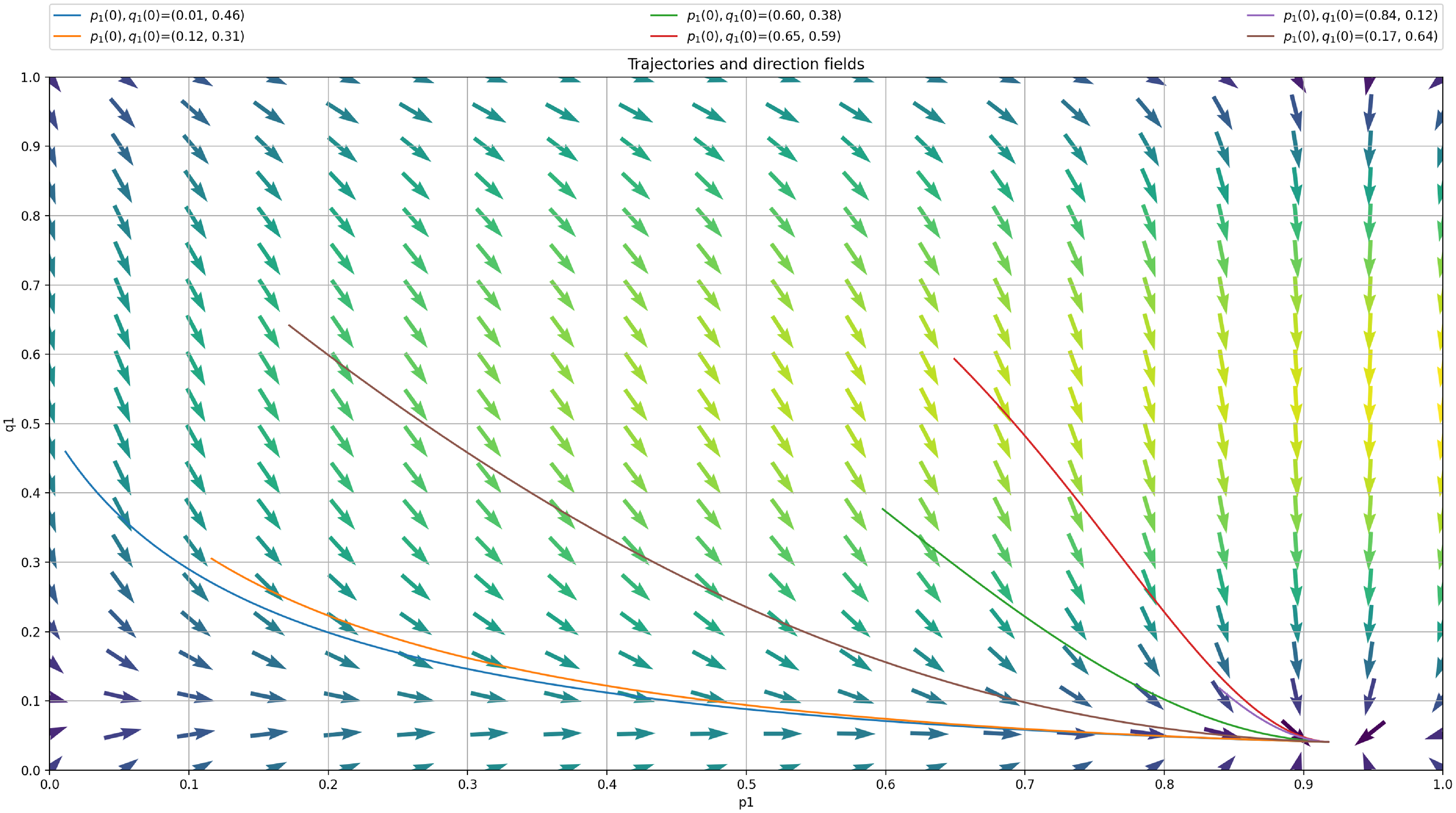


Observing the small dispersancy between
 $(p^*,q^*)=(0.917, 0.040)$
and
$(p^*,q^*)=(0.917, 0.040)$
and
 $(p_{opt},q_{opt})=(1, 0)$
from the ODE and from the LA trajectory as shown in Figures 6 and 7 motivates us to choose even a larger value of
$(p_{opt},q_{opt})=(1, 0)$
from the ODE and from the LA trajectory as shown in Figures 6 and 7 motivates us to choose even a larger value of
 $p_{max}$
. Thus, we increase
$p_{max}$
. Thus, we increase
 $p_{max}$
from
$p_{max}$
from
 $0.99$
to
$0.99$
to
 $0.999$
and observe the expected convergence results from the ODE in Figure 8. We observe a single attraction point close of the ODE close to the pure Nash equilibrium. We can read from the ODE trajectory that
$0.999$
and observe the expected convergence results from the ODE in Figure 8. We observe a single attraction point close of the ODE close to the pure Nash equilibrium. We can read from the ODE trajectory that
 $(p^*,q^*)=(0.991, 0.004)$
which is closer
$(p^*,q^*)=(0.991, 0.004)$
which is closer
 $(p_{opt},q_{opt})=(1, 0)$
than the previous case with a smaller
$(p_{opt},q_{opt})=(1, 0)$
than the previous case with a smaller
 $p_{max}$
.
$p_{max}$
.
Trajectory of ODE using
 $p_{max}=0.999$
for case 2.
$p_{max}=0.999$
for case 2.
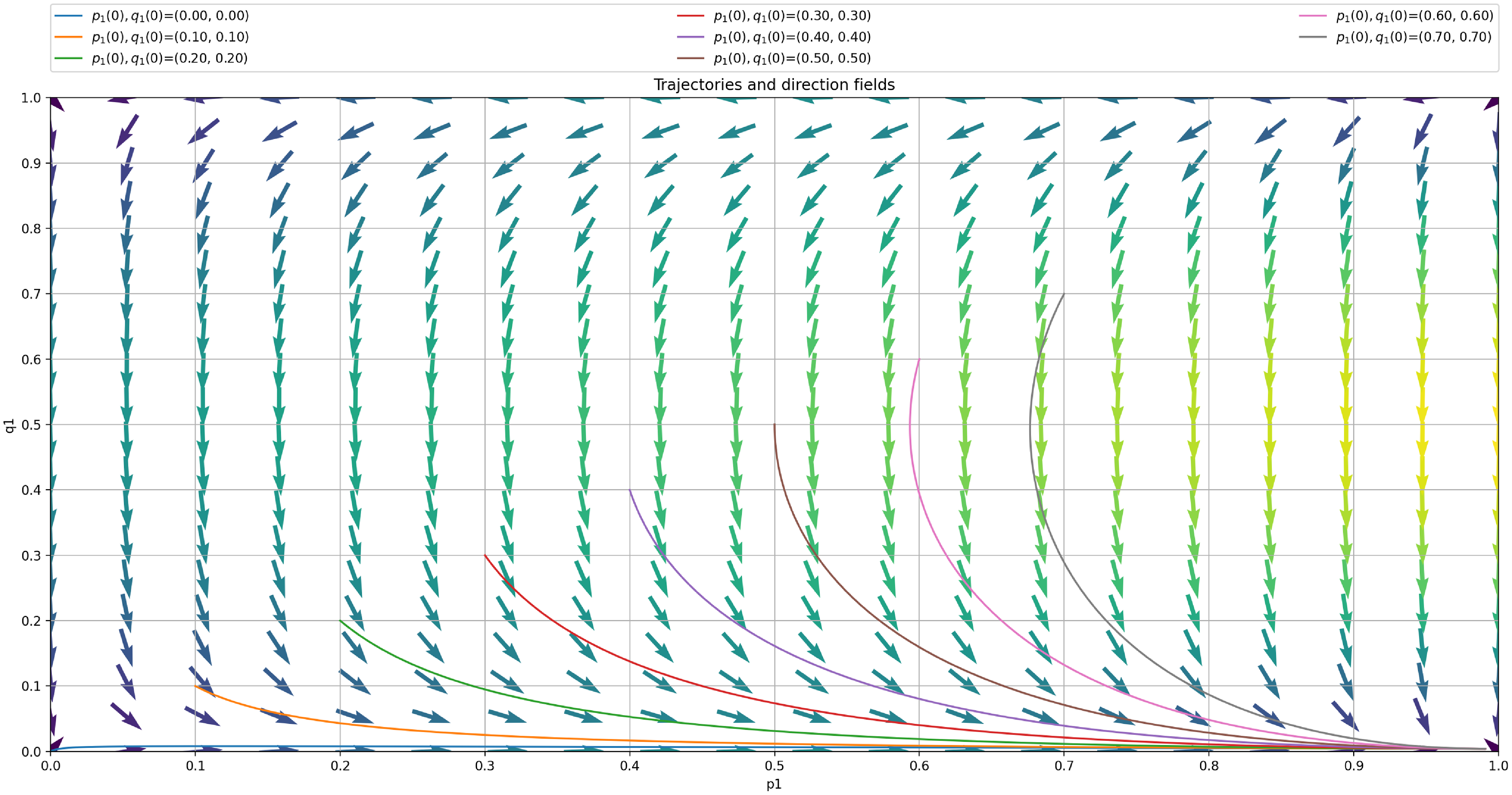
In Figure 9a, we depict the time evolution of the two components of the vector X(t) using the proposed algorithm for an ensemble of 1000 runs. In the case of having a Pure Nash equilibrium, there is no oscillatory behavior as when a player assigns more probability to an action, since the other player reinforces the strategy. However, Figure 9a could mislead the reader to believe that the LA method has converged to a pure strategy for both players. In order to clarify that we are not converging to an absorbing state for the player A, we provide Figure 9b which zooms on Figure 9a around the region where the strategy of player A has converged in order to visualize that its maximum first action probability is limited by
 $p_{max}$
, as per the design of our updating rule. Similarly, we zoom on the evolution of the first action probability of player B in Figure 9c. We observe that the first action instead to converging to zero as it would be if we did not have absorbing barriers, its rather converges to a small probability limited by
$p_{max}$
, as per the design of our updating rule. Similarly, we zoom on the evolution of the first action probability of player B in Figure 9c. We observe that the first action instead to converging to zero as it would be if we did not have absorbing barriers, its rather converges to a small probability limited by
 $p_{min}$
which approaches zero. Such propriety of evading lock in probability even for pure optimal strategies and which emanates from the ergodicity of our
$p_{min}$
which approaches zero. Such propriety of evading lock in probability even for pure optimal strategies and which emanates from the ergodicity of our
 $L_{R-I}$
scheme with absorbing barriers is a desirable property specially when the payoff matrices are time-varying and thus the optimal equilibrium point might change over time. Such a case deserves a separate study to better understand the behavior of the scheme and to also understand the effect of the tuning parameters and how to control and vary them in this case to yield a compromise between learning and forgetting stale information.
$L_{R-I}$
scheme with absorbing barriers is a desirable property specially when the payoff matrices are time-varying and thus the optimal equilibrium point might change over time. Such a case deserves a separate study to better understand the behavior of the scheme and to also understand the effect of the tuning parameters and how to control and vary them in this case to yield a compromise between learning and forgetting stale information.
The figure shows (a) the evolution over time of X(t) for
 $\theta=0.01$
and
$\theta=0.01$
and
 $p_{max}=0.999$
when applied to game with payoffs specified by the R matrix and the C matrix given by Equation (6.5) and Equation (6.6), and (b) is a zoomed version around player A strategy c) and is a zoomed version around player B strategy.
$p_{max}=0.999$
when applied to game with payoffs specified by the R matrix and the C matrix given by Equation (6.5) and Equation (6.6), and (b) is a zoomed version around player A strategy c) and is a zoomed version around player B strategy.
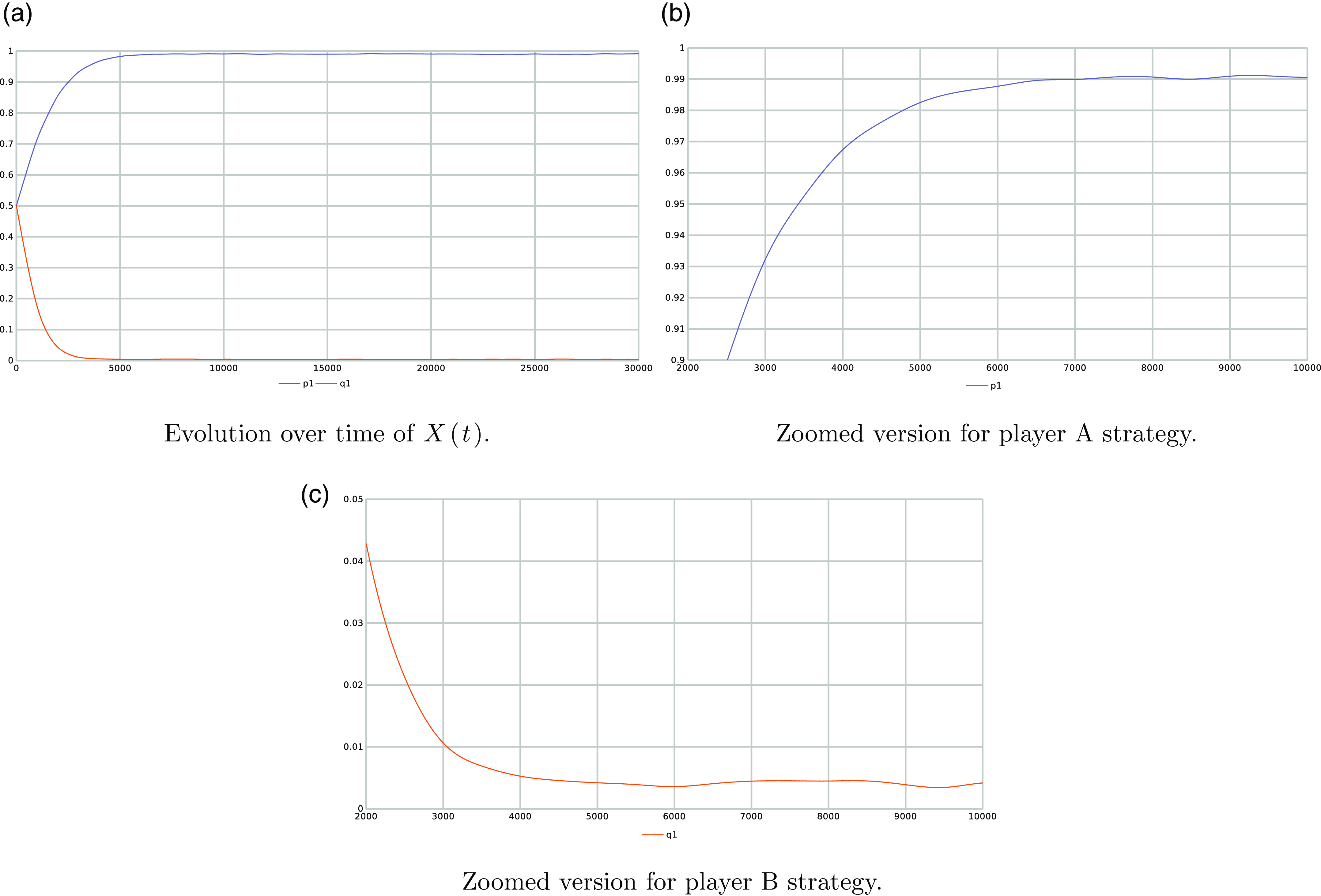
Figure 9 depicts the time evolution of the probabilities for each player, with
 $\theta=0.01$
,
$\theta=0.01$
,
 $p_{max}=0.999$
and for an ensemble with 1000 runs.
$p_{max}=0.999$
and for an ensemble with 1000 runs.
6.3. Case 3: 2 Pure equilibria and 1 mixed
Now, we shall consider the last case 3.
As an instance of case 3, we consider the payoff matrices R and C given by:
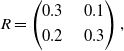 \begin{equation}R=\begin{pmatrix}0.3 & \quad 0.1 \\[3pt] 0.2 & \quad 0.3\end{pmatrix},\end{equation}
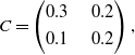 \begin{equation}C=\begin{pmatrix} 0.3 & \quad 0.2 \\[3pt] 0.1 & \quad 0.2 \end{pmatrix},\end{equation}
In Figure 10, we plot 9 trajectories for the LA for a number of iterations is 1 000 000. We observe that depending on the initial conditions, our LA converges to one of the two pure equilibria which is usually the closest to the starting point. We have also performed extensive simulations with initial values
 $(0.5, 0.5)$
of the probabilities and we found that almost 50% of the time the LA converges to the Nash equilibrium close to (1,1) and 50% close to (0,0). As a future work, we would like to explore how to push the LA to favor one of the two equilibria as there is usually an equilibrium that is superior to the other, and thus it is more desirable for both players to converge to the superior Nash equilibrium.
$(0.5, 0.5)$
of the probabilities and we found that almost 50% of the time the LA converges to the Nash equilibrium close to (1,1) and 50% close to (0,0). As a future work, we would like to explore how to push the LA to favor one of the two equilibria as there is usually an equilibrium that is superior to the other, and thus it is more desirable for both players to converge to the superior Nash equilibrium.
9 Trajectories of the LA with barriers starting from random initial point with
 $p_{max}=0.99$
and
$p_{max}=0.99$
and
 $\theta=0.0001$
.
$\theta=0.0001$
.
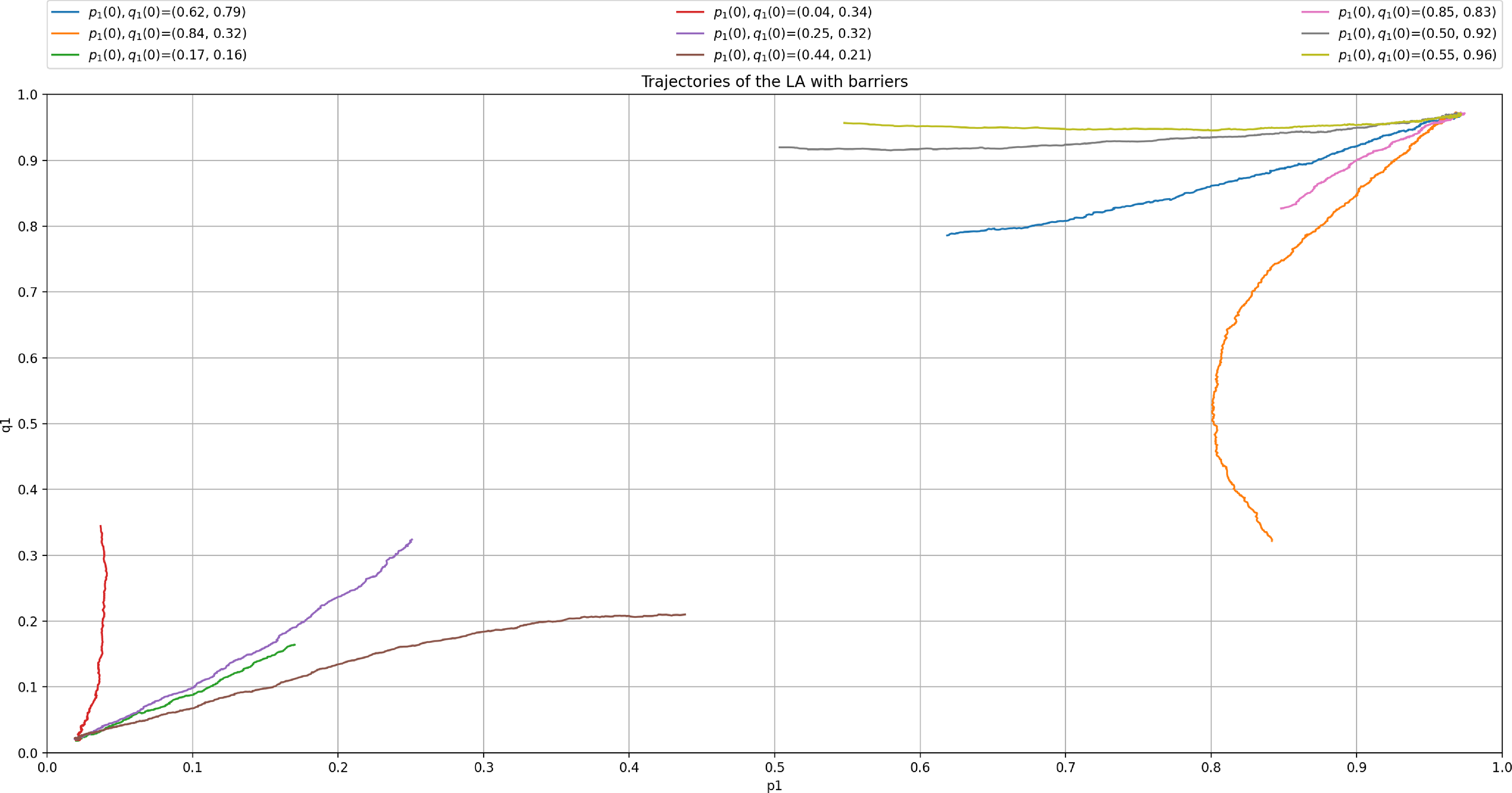
We plot the ODE corresponding to our LA for case 3 in Figure 11. We can see two attractions points which approach the two Nash equilibria.
Trajectory of ODE using
 $p_{max}=0.99$
for case 3.
$p_{max}=0.99$
for case 3.
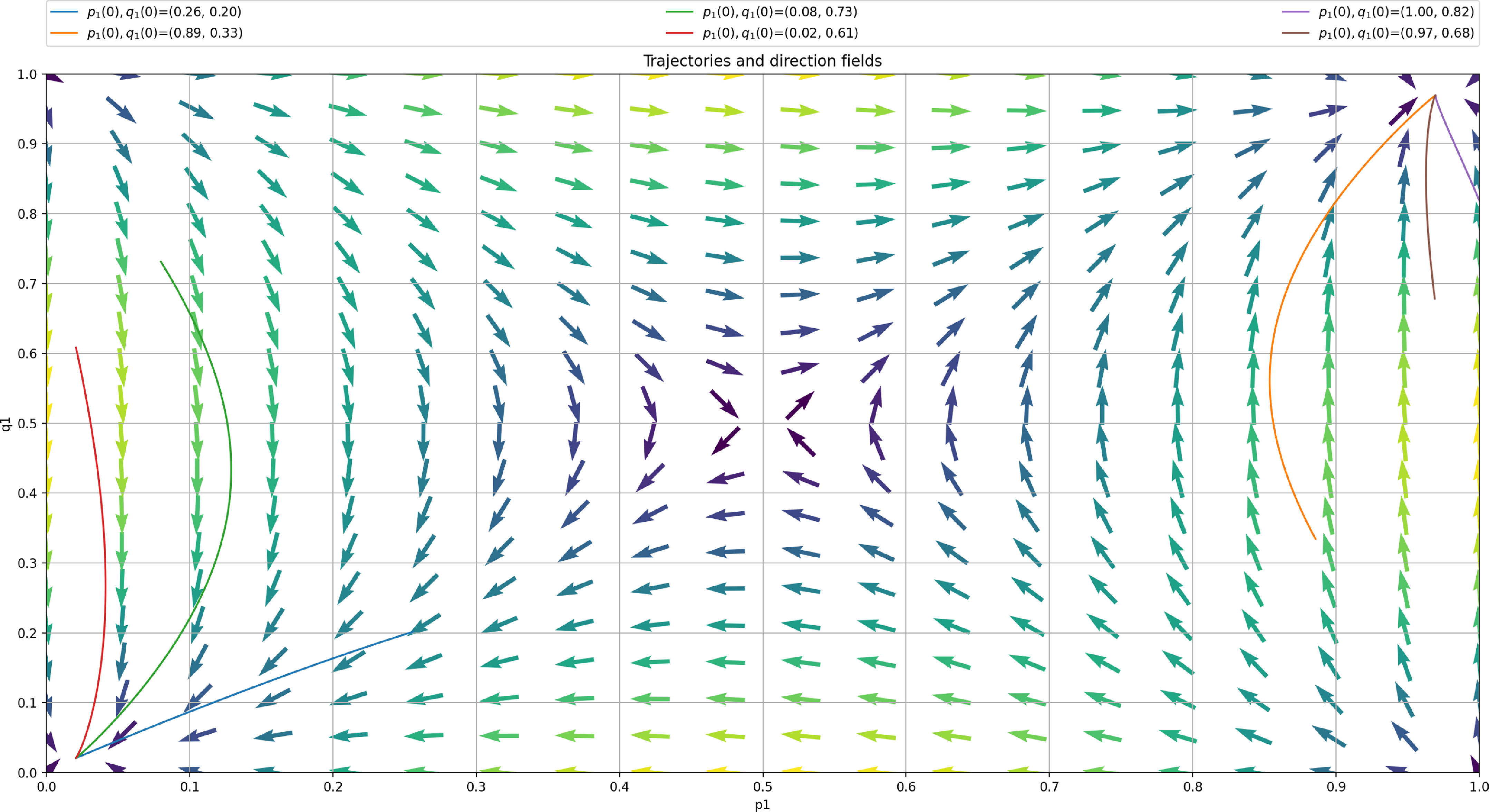
Although for

 $p_{max} \neq 1$
, w our scheme is in theory ergodic and not absorbing, this is not the case in practice as shown in the simulation reported in Table 3. In fact for
$p_{max} \neq 1$
, w our scheme is in theory ergodic and not absorbing, this is not the case in practice as shown in the simulation reported in Table 3. In fact for
 $\theta=0.0001$
and as
$\theta=0.0001$
and as
 $p_{max}$
becomes larger or equal to
$p_{max}$
becomes larger or equal to
 $0.995$
, we observe that the error is zero meaning that the LA has converged already to an absorbing state! This lock in probability phenomenon is due to the limited accuracy of the machine and limitations of the random number generator. For smaller
$0.995$
, we observe that the error is zero meaning that the LA has converged already to an absorbing state! This lock in probability phenomenon is due to the limited accuracy of the machine and limitations of the random number generator. For smaller
 $\theta=0.00001$
, we expect that the LA will approximate better the ODE. Indeed, this is the case the absorption this time does not happen for
$\theta=0.00001$
, we expect that the LA will approximate better the ODE. Indeed, this is the case the absorption this time does not happen for
 $p_{max}=0.995$
and
$p_{max}=0.995$
and
 $p_{max}=0.996$
as in the previous case, but happen for only
$p_{max}=0.996$
as in the previous case, but happen for only
 $p_{max}$
larger or equal to
$p_{max}$
larger or equal to
 $p_{max}=0.997$
.
$p_{max}=0.997$
.


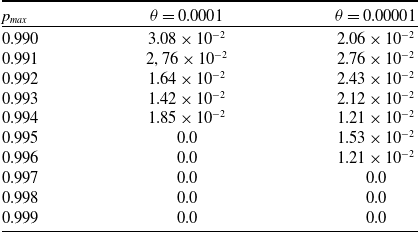
Solving the ODE for
 $p_{max}=0.999$
, gives two solutions, namely,
$p_{max}=0.999$
, gives two solutions, namely,
 $(p^*,q^*)=(0.99699397,0.99699397)$
and
$(p^*,q^*)=(0.99699397,0.99699397)$
and
 $(0.00200603,0.00200603)$
which approach
$(0.00200603,0.00200603)$
which approach
 $(p_{\mathrm{opt}},q_{\mathrm{opt}})=(1,1)$
and
$(p_{\mathrm{opt}},q_{\mathrm{opt}})=(1,1)$
and
 $(p_{\mathrm{opt}},q_{\mathrm{opt}})=(0,0)$
respectively.
$(p_{\mathrm{opt}},q_{\mathrm{opt}})=(0,0)$
respectively.
Solving the ODE for
 $p_{max}=0.998$
, gives two solutions
$p_{max}=0.998$
, gives two solutions
 $(p^*,q^*)=(0.99397576,0.99397576)$
and
$(p^*,q^*)=(0.99397576,0.99397576)$
and
 $(0.00402424,0.00402424)$
.
$(0.00402424,0.00402424)$
.
While solving the ODE for
 $p_{max}=0.997$
, gives
$p_{max}=0.997$
, gives
 $(p^*,q^*)=(0.99094517,0.99094517)$
and
$(p^*,q^*)=(0.99094517,0.99094517)$
and
 $(0.00605483,0.00605483)$
.
$(0.00605483,0.00605483)$
.
7. Experimental results for S-type environments
In this section, we present the results of the experiments for the S-type learning game. We conducted several simulations similar to those presented in Section 6. The same instances of the payoff matrices R and C were used, covering the cases referred to in Section 4.
For all the experiments conducted for the S-LA, 9 trajectories were plotted for 2 000 000 iteration, with
 $p_{max}=0.99$
and
$p_{max}=0.99$
and
 $\theta=0.0001$
. A general observation that we noticed when performing that the experiments is that the S-LA converges slower than the
$\theta=0.0001$
. A general observation that we noticed when performing that the experiments is that the S-LA converges slower than the
 $L_{R-I}$
. Therefore, we have doubled the number of iterations to allow the S-LA to converge in our experiments.
$L_{R-I}$
. Therefore, we have doubled the number of iterations to allow the S-LA to converge in our experiments.
7.1. Case 1: Only one mixed Nash equilibrium exists
Figure 12 depicts the situation where the only Nash equilibrium that exists is a mixed one. We can easily observe that the S-LA approaches the trajectories of the ODE given in Figure 5. Please note that the ODE regardless of the LA type, whether it is
 $L_{R-I}$
or
$L_{R-I}$
or
 $S-$
LA.
$S-$
LA.
Trajectory of S-LA using
 $p_{max}=0.99$
and
$p_{max}=0.99$
and
 $\theta=0.0001$
for case 1.
$\theta=0.0001$
for case 1.
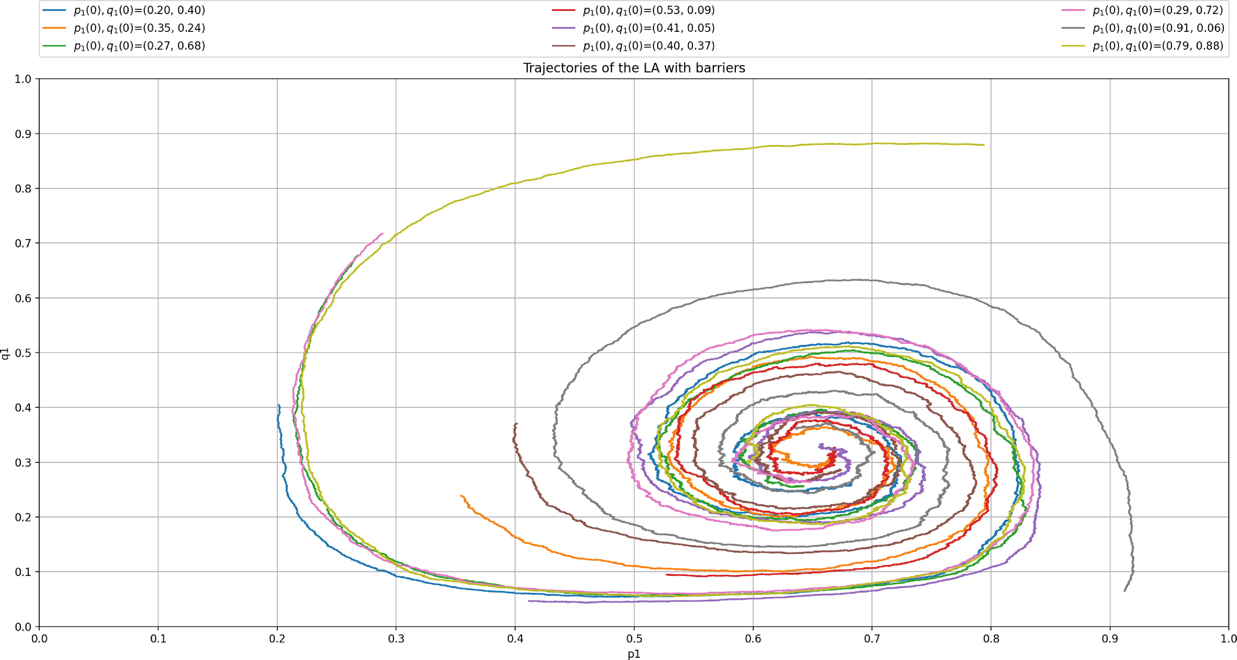
7.2. Case 2: One pure equilibrium
We also examined the case where the game has a single pure equilibrium. The exhibited behavior is comparable to those reported in Section 6. The trajectory of the LA depicted in Figure 13 tightly follows the trajectories of the ODE depicted in Figure 6. As
 $\theta$
goes to zero, the trajectories of the LA and those of the ODE will be indistinguishable (Sastry et al., Reference Sastry, Phansalkar and Thathachar1994).
$\theta$
goes to zero, the trajectories of the LA and those of the ODE will be indistinguishable (Sastry et al., Reference Sastry, Phansalkar and Thathachar1994).
Trajectory of S-LA using
 $p_{max}=0.99$
and
$p_{max}=0.99$
and
 $\theta=0.0001$
for case 2.
$\theta=0.0001$
for case 2.
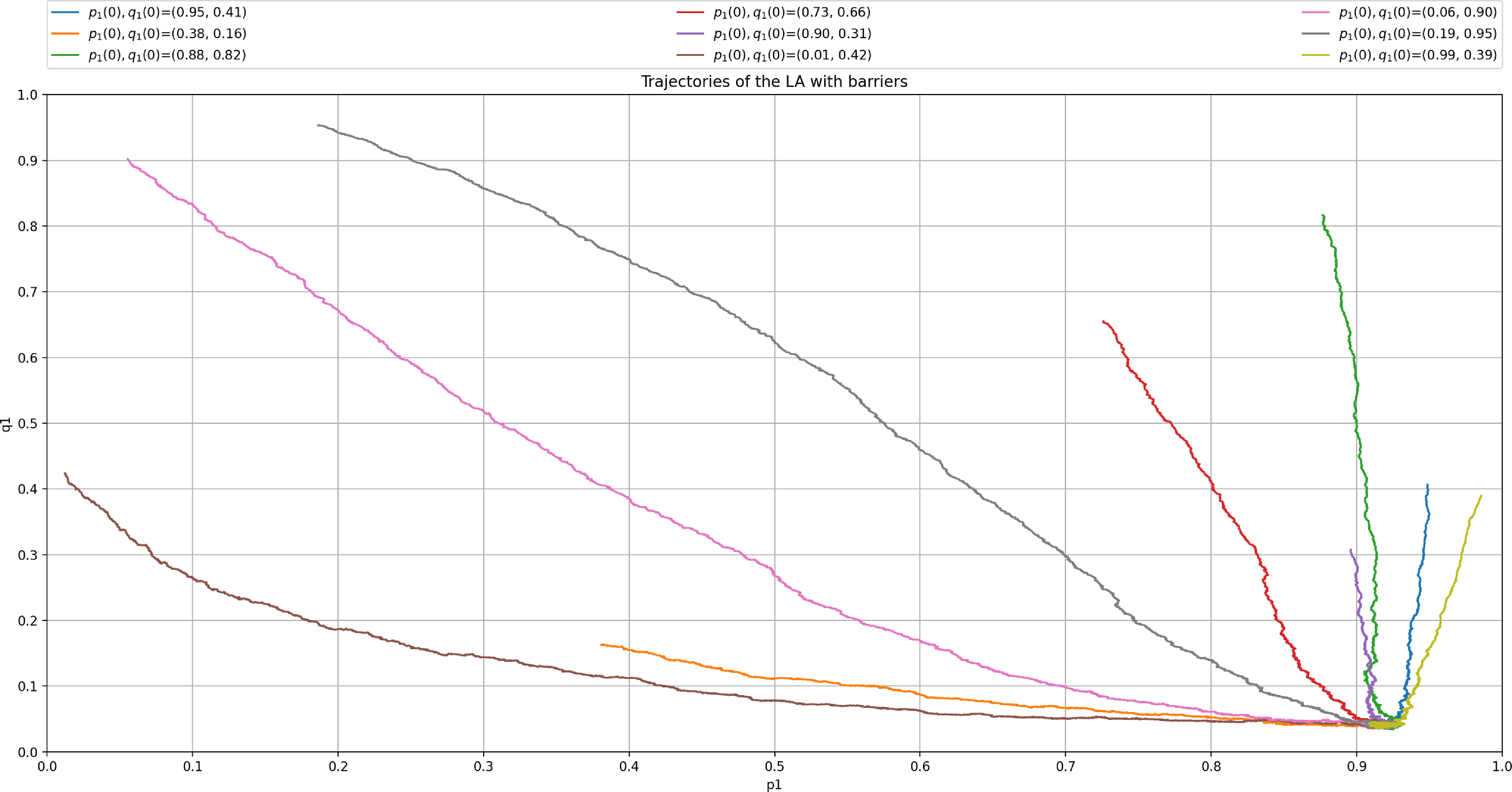
7.3. Case 3: Two pure equilibria and one mixed
Figure 14 shows the situation where there are two pure equilibria and one mixed.
Trajectory of S-LA using
 $p_{max}=0.99$
and
$p_{max}=0.99$
and
 $\theta=0.0001$
for case 3.
$\theta=0.0001$
for case 3.
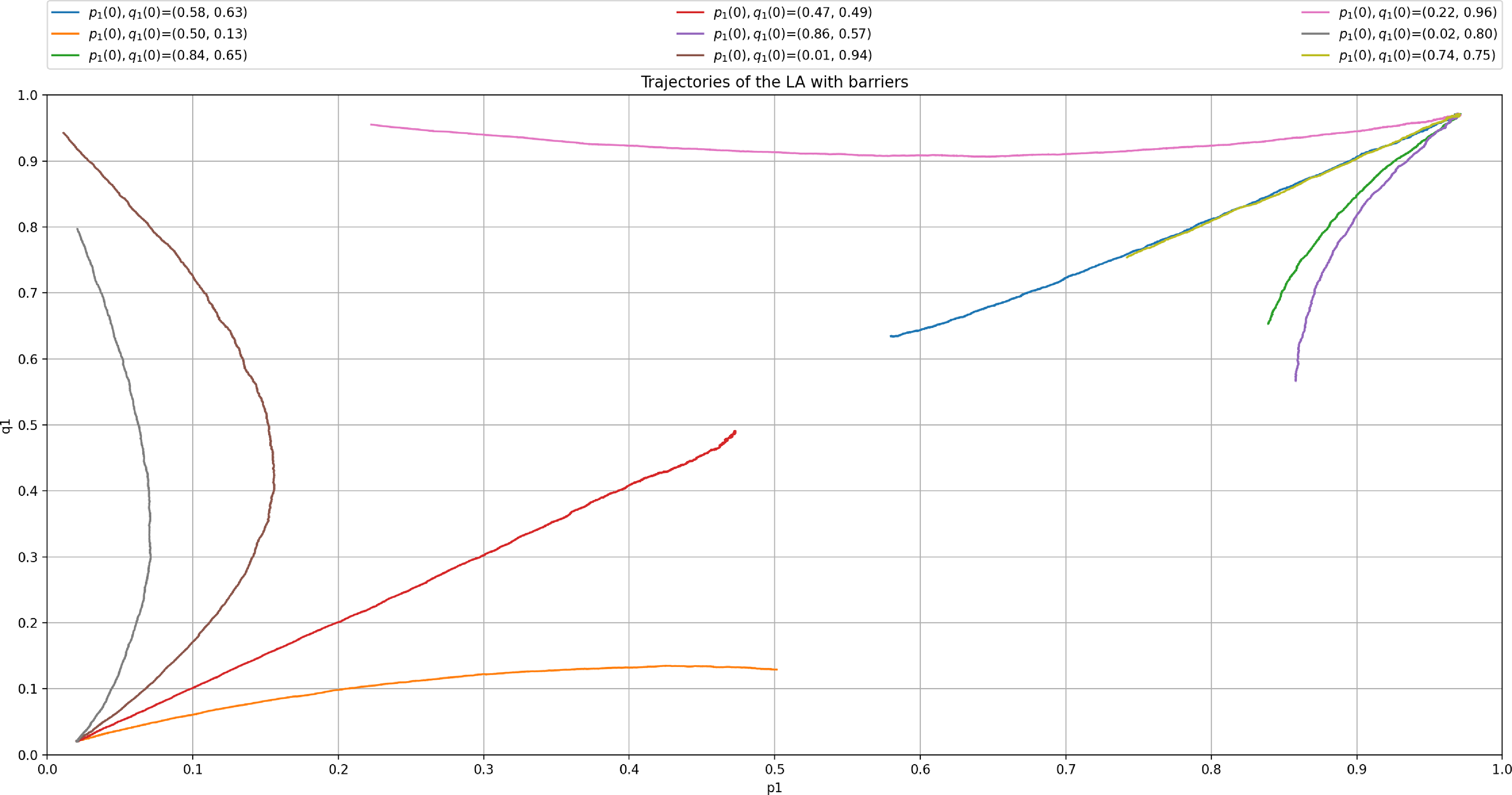
We observe that the LA converges to one of the two pure equilibria that is closest to the starting point. The S-LA behaves much similar to the
 $L_{R-I}$
LA as shown in Figure 10. We also observe that the S-LA respectively converged to the Nash equilibrium close to (1, 1) and close to (0,0) approximately 50% of the time.
$L_{R-I}$
LA as shown in Figure 10. We also observe that the S-LA respectively converged to the Nash equilibrium close to (1, 1) and close to (0,0) approximately 50% of the time.
Appendices
Appendix A. Norman theorem
Theorem 5. Let X(t) be a stationary Markov process dependent on a constant parameter
 $\theta \in [0,1]$
. Each
$\theta \in [0,1]$
. Each
 $X(t) \in I$
, where I is a subset of the real line. Let
$X(t) \in I$
, where I is a subset of the real line. Let
 $\Delta X(t)=X(t+1)-X(t)$
. The following are assumed to hold:
$\Delta X(t)=X(t+1)-X(t)$
. The following are assumed to hold:
-
1. I is compact.
-
2.
$E [\Delta X(t) | X(t)=y]= \theta w(y)+ O(\theta^2)$
-
3.
$Var [\Delta X(t) | X(t)=y]= \theta ^2 s(y)+ o(\theta ^2)$
-
4.
$E [\Delta X(t)^3 | X(t)=y]= O(\theta ^3)$
where
$sup_{y \in I} \frac{O(\theta^k)}{\theta^k}< \infty$
for
$K=2,3$
and
$sup_{y \in I} \frac{o(\theta^2)}{\theta^2} \rightarrow 0$
as
$\theta \rightarrow 0$
. -
5. w(y) has a Lipschitz derivative in I.
-
6. s(y) is Lipschitz I.


If Assumptions (1)-(6) hold, w(y) has a unique root
 $y^*$
in I and
$y^*$
in I and
 $\frac{d w}{d y} \bigg|_{y=y^*} \le 0$
then
$\frac{d w}{d y} \bigg|_{y=y^*} \le 0$
then
-
1.
$var [\Delta X(t) | X(0)=x]=0(\theta)$
uniformly for all
$x \in I$
and
$t \ge 0$
. For any
$x \in I$
, the differential equation
$\frac{d y(\tau)}{d \tau}=w(y(t))$
has a unique solution
$y(\tau)=y(\tau,x)$
with
$y(0)=x$
and
$E [\delta X(t) | X(0)=x]=y( t \theta)+O(\theta)$
uniformly for all
$x \in I$
and
$t \ge 0$
. -
2.
$\frac{X(t)-y(t \theta)}{\sqrt \theta}$
has a normal distribution with zero mean and finite variance as
$\theta \rightarrow 0$
and
$t \theta \rightarrow \infty$
.


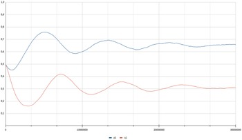


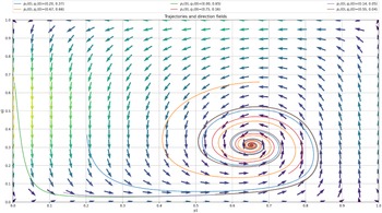

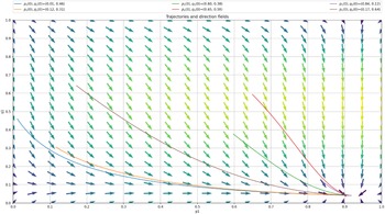

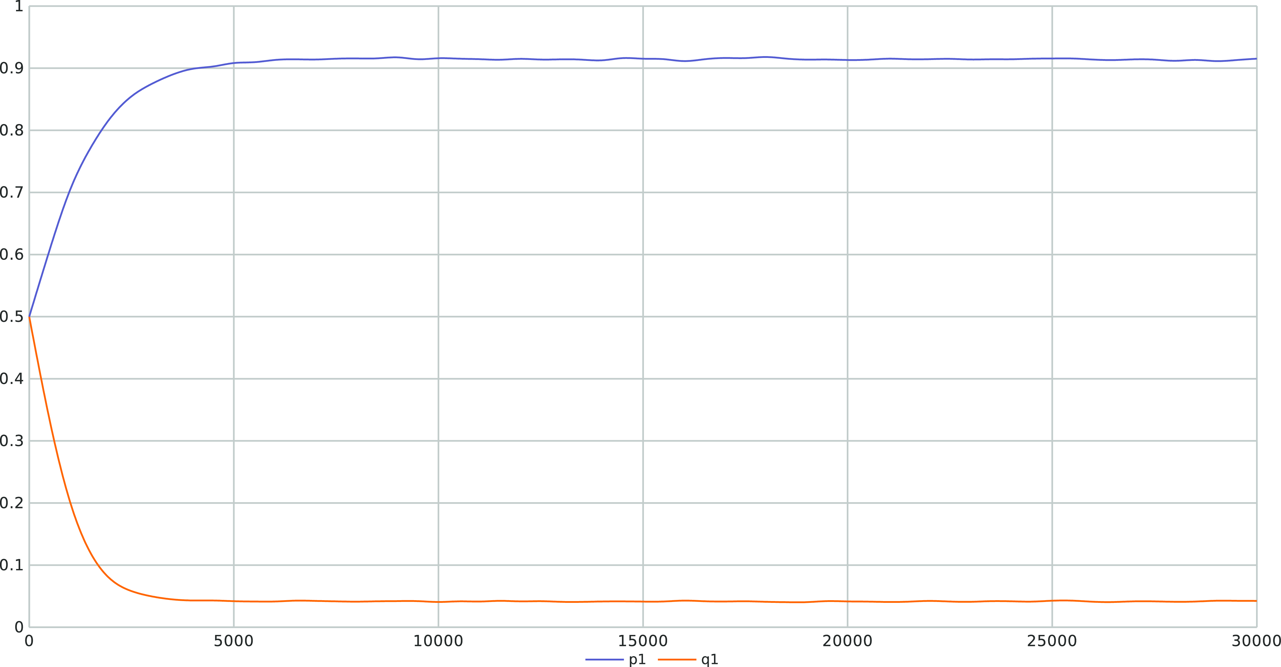


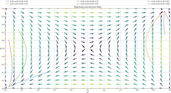


 Open access