

Introduction
Reference Holdsworth and JacobsHoldsworth (1985) analyzed different sources of ocean forcing that could cause calving on floating glacier tongues such as that of Mertz Glacier, East Antarctica (Fig. 1). Depending on the region, there are a number of possible mechanisms including tsunami wave interaction, storm wave interaction (storm surge wave) (Reference Zumberge and SwithinbankZumberge and Swithinbank, 1962;Reference Bromirski, Sergienko and MacAyealBromirski and others, 2010), pressure induced by long ocean waves with shelf amplification, collision between icebergs and floating ice tongues (Reference Swithinbank, McClain and LittleSwithinbank and others, 1977), and tidal motion (Reference Zumberge and SwithinbankZumberge and Swithinbank, 1962).
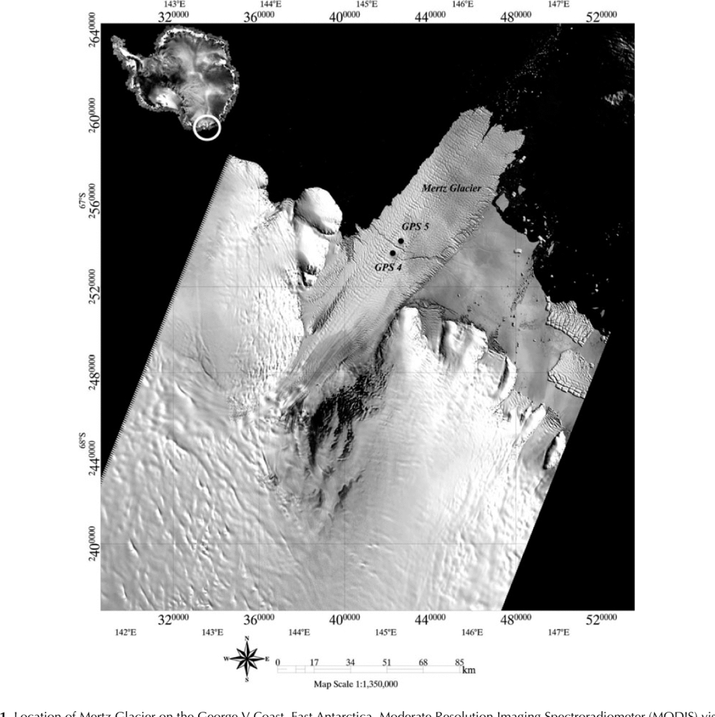
Location of Mertz Glacier on the George V Coast, East Antarctica. Moderate Resolution Imaging Spectroradiometer (MODIS) visible image from 16 March 2009 projected with a 10 km spacing grid overlaid.
Ocean wave energy is one of the primary mechanisms described by Reference Holdsworth and JacobsHoldsworth (1985) that lead to glacier ice- tongue calving. The ocean wave spectrum arrives and interacts with the glacier, which then acts like a filter, with filtering characteristics depending on the ice thickness (Reference Holdsworth and GlynnHoldsworth and Glynn, 1981).
When a dominant frequency occurring in the incident wave spectrum coincides with one of the natural frequencies of the ice tongue, cyclic bending stresses may lead to crack propagation and fatigue failure in the ice. Hence it is of some interest to examine the oscillation characteristics of floating ice tongues and in particular to look at their natural frequencies to investigate the possibility of resonance with the ocean waves and to learn more about calving processes.
The Collaborative Research into Antarctic Calving and Iceberg Evolution (CRAC-ICE) project was developed during the International Polar Year (http://ipv.articportal.org/) to understand the mechanics of ice-shelf rift initiation and propagation via three complementary components: field work, satellite data analysis and ice-shelf/ocean modeling. An additional objective of CRAC-ICE was the monitoring of iceberg evolution as icebergs drift away from their calving site. It is in this context that during the Institut Paul-Emile Victor (IPEV) R0 Astrolabe voyage of November 2007 we deployed a network of six GPS receivers along a flowline of Mertz Glacier. Two months of GPS data were collected at the end of the field season from two stations, GPS4 and GPS5 (Fig. 1), situated on each side of the main rift of the glacier ice tongue, and three base stations (Commonwealth Bay, Penguin Point and Close Island) were installed on rocks around Mertz Glacier. The data from the base stations were collected during November 2009.
Before analyzing these GPS data in detail, we first used a number of different GPS software and processing strategies in order to obtain the best possible accuracy with the aim of reliably resolving cm-scale movement. We investigated the oscillating signals recorded by our GPS receivers located on ice, and characterized these vibrations using a simple elastic- beam model. Finally, we compared the vibrations recorded by GPS4 (south of the main rift) and GPS5 (north of the main rift) to learn more about their impact on the rift propagation and the possible impact on the calving mechanism.
Study Area
Located in King George V Land, East Antarctica, 200 km from the French base station Dumont d'Urville, Mertz Glacier has a prominent ice tongue 35 km in width with ice thicknesses from 300 to 1200 m along its length (Fig. 1). This ice tongue extends over 100 km into the open ocean, with a total length of ˜150 km. Several attempts have been made to measure the ice discharge of the glaciers in this region, including that by Reference Frezzotti, Cimbelli and FerrignoFrezzotti and others (1998), who estimated the accumulated discharge of Mertz and Ninnis Glaciers to be 62 Gta-1 and the ice accumulation in the drainage basin to be 58Gta-1 calculated from Landsat images over the period 1989-91. Reference RignotRignot (2002) calculated a drainage basin area of 83 080 km2 for Mertz Glacier. Reference Wendler, Ahlnas and LingleWendler and others (1996) used a synthetic aperture radar (SAR) image pair separated by 19 months to determine the velocity of Mertz Glacier ice tongue. A mean value of 1020m a-1 was calculated and it was suggested that no significant difference exists between the long- (decadal) and short-term (yearly) ice velocity trends.
In addition, Reference Legresy, Wendt, Tabacco, Remy and DietrichLegresy and others (2004) found that the along-flow velocity of Mertz Glacier ice tongue varied from 1.9 to 6.8 md-1 depending on the direction of the tidal current at the ice tongue. They used interferometric SAR (InSAR) data from 1996 and GPS records from 2000, and deduced from these records that large variations of flow speed, in phase with tidal cycles, may be linked to a variation in friction of the ice on the eastern rocky wall.
The main feature of Mertz Glacier is its active rift, which played an important role in the most recent calving event between 12 and 13 February 2010. Before this period, very little information existed about previous calving events. Reference Frezzotti, Cimbelli and FerrignoFrezzotti and others (1998) showed that the evolution of the length of the ice tongue was not continuous: from 150 km in 1912, it reduced to 113 km in 1958 and increased again to 155 km in 1996. They concluded that at least one major calving event occurred between 1912 and 1956.
In the case of the Mertz Glacier calving event in 2010, a collision with the B09B iceberg, driven by ocean currents, played a major role. However, even if this iceberg collision was the final instigator of the calving of Mertz Glacier ice tongue, the two rifts at both sides of the glacier were already well developed at some distance from the grounding line, at locations where one might expect the bending moments and stresses to be largest and thus these rifts to have been at the origin of the calving (Reference LescarmontierLescarmontier, 2012).
Vertical Movements of the Ice Tongue Datasets
Datasets
The data available for analysis in this study come mainly from the 2007/08 CRAC-ICE fieldwork season. They include GPS data from two receivers on the ice tongue each side of the main rift (GPS4 and 5) and from two receivers on rock sites each side of the glacier (Penguin Point and Close Island). We also used data from a rock site in Common wealth Bay ˜65 km away (Table 1).
Dataset: available data and location of the GPS receivers
Topcon GB1000 dual frequency receivers, set at 30 s sampling rate, and PGA1 antennas were used. The Close Island rock site antenna mounts consisted of 48 mm diameter steel tubes installed in the rock. For Penguin Point, we reoccupied the geodetic marker installed by the GANOVEX VIII 2000 expedition (Geology and Geophysics of Marie Byrd Land, Northern Victoria Land and Oates Coast). The Commonwealth Bay station was installed on a Geoscience Australia geodetic benchmark. For Mertz Gla cier sites, the antenna mount was a wooden pole buried 1.6m in the snow with intermediate wooden feet. This style of glacier GPS site ensures the stability of the antenna with very low sensitivity to melt.
Processing the data
Our results show that accurate GPS processing at the centimeter level can be achieved. Here we demonstrate a new GPS technique that allows us to achieve this level of accuracy for our GPS solutions.
From raw data to accurate position, we tried various GPS processing strategies and software in order to evaluate the accuracy level that we could achieve. We used the CSRS-PPP online processing tool from NRCAN (http://ess.nrcan.gc.cs/2002_2006/gnd/csrs_f.php), the GINS geodetic software from CNES-GRGS (version 5 July 2009; http://www.igsac-cnes.cls.fr/document/gins/GINS_Doc_Algo.html) and the TRACK kinematic module of GAMIT (Reference ChenChen, 1998; Reference HerringHerring, 2009).
The processing strategy used was based on the double difference (DD) carrier phase technique or the Precise Point Positioning (PPP) technique, depending on the capabilities of the selected software: CSRS-PPP offers only PPP processing, TRACK is based on a differential processing approach and GINS can process GPS data using both techniques. Because DD eliminates common receiver and satellite biases, the remaining DD phase ambiguity is an integer that can be recovered using one of the numerous algorithms already published. It is well known that fixing ambiguities to integers improves the solution (Reference BlewittBlewitt, 1989;Reference BertigerBertiger and others, 2010). Cancellation of GPS errors reduces and this improve ment is generally in the east component with longer (>20- 50 km) baselines, although precise time series have been reported over much longer baselines (Reference Anandakrishnan, Voigt, Alley and KingAnandakrishnan and others, 2003). The PPP approach is an interesting alternative processing approach as it does not require a base station (Reference Zumberge, Heflin, Jefferson, Watkins and WebbZumberge and others, 1997), taking advantage of pre computed and precise satellite orbits and clocks. However, 'classical' PPP algorithms are based on float (real) phase ambiguity solutions (Reference King and AokiKing and Aoki, 2003;Reference Zhang and AndersenZhang and Andersen, 2006). Several authors have recently demon strated the ability to deal with the satellite and receiver biases in order to recover the integer nature of the zero-difference ambiguities (Reference Ge, Gendt, Rothacher, Shi and LiuGe and others, 2008; Reference Laurichesse, Mercier, Berthias, Broca and CerriLaurichesse and others, 2009;Reference Geng, Meng, Dodson and TeferleGeng and others, 2010). As a consequence, 'integer PPP' (here named IPPP) is now possible. This alternative technique typically has the same level of accuracy as DD and is not limited by baseline length considerations. IPPP capability has been implemented in the GINS software, but a priori dedicated precise satellite orbit, clocks and biases are needed. These products are part of the official contribution of the CNES-CLS (Collecte, Localisation, Satellites) IGS Analy sis Center and are freely available (under the acronym GRGS) (Reference Loyer, Perosanz, Capdeville and SoudarinLoyer and others, 2009).
The PPP kinematic time series were computed at 30s sampling with GINS. We used IGS (International GNSS (global navigation satellite systems)) products for the float GINS-PPP processing (Reference Dow, Neilan and RizosDow and others, 2009) but GRGS- IGS(http:\\www.igsc-cnes.cls.fr) precise orbits and (30 s) clock products for the GINS-IPPP processing.
The 'ionospheric-free' linear combination of L1 and L2 GPS observations was used with a 10° satellite elevation cut off applied. The GPT pressure model (Reference Boehm, Heinkelmann and SchuhBoehm and others, 2007) and GMF mapping function (Reference Boehm, Niell and Tregoning Pand SchuhBoehm and others, 2006) were used. Antenna eccentricities as well as phase center variations derived from igs05.atx conventions were used.
In the case of the CSRS, TRACK and GINS software, the following data weighting was applied for range and phase observations, respectively: CSRS (2 m;1.5 cm), TRACK (3 m; 1 mm), GINS (35 cm;3.5 mm), with data weighting proportional to cos(elevation)2 for both range and phase. Finally we corrected for the solid-earth tide and ocean tide loading terms (using the finite-element solutions (FES) 2004 with Internal Earth Rotation Service (IERS) conventions) in our GPS time series.
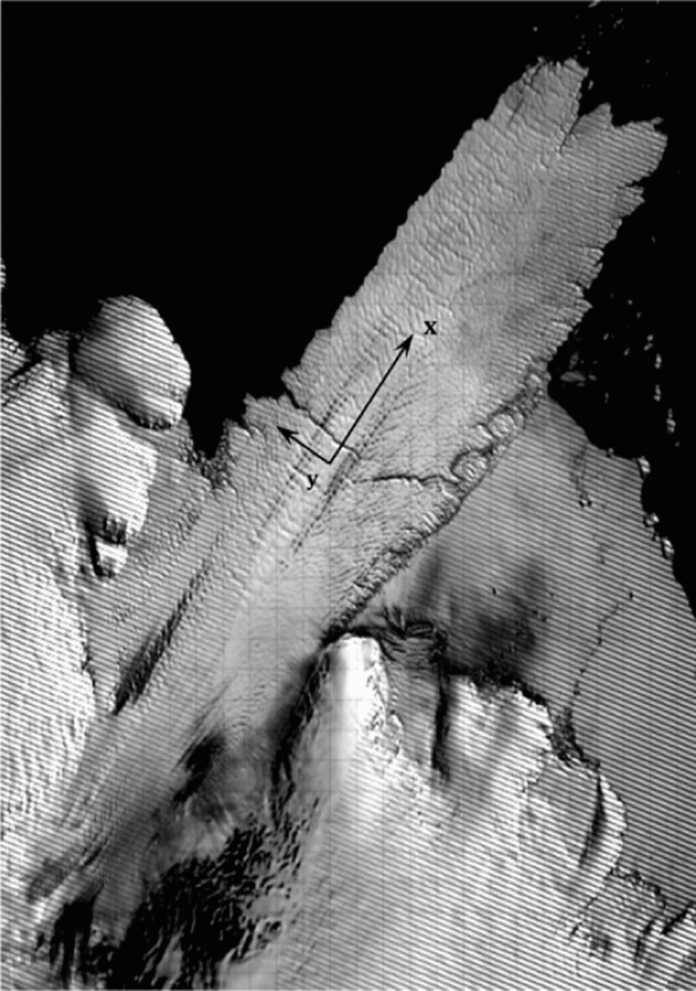
The results of the GPS processing were determined in Cartesian geocentric coordinates in the ITRF2005 (Reference Altamimi, Collilieux, Legrand, Garayt and BoucherAltamimi and others, 2007). We projected our solutions into a local topocentric coordinate system: along-flow (x direction), across-flow (y direction) and the local up direction (vertical) (Fig. 2).
Coordinate axes (along, across, height) on a Landsat image of Mertz Glacier (from 12 December 2006).
The second part of the data analysis focused on the local topocentric components of the signal. Mertz Glacier ice tongue is floating on the ocean, so the two main signals were the horizontal (x, y) glacier flow (˜3md_1) and the vertical (z) tidal signal (Reference Legresy, Wendt, Tabacco, Remy and DietrichLegresy and others, 2004). The horizontal displacement associated with the ice flow increases mono- tonically through time and is easily detrended. To remove the tides, we used a tidal harmonic analysis program (Reference Lyard, Lefevre, Letellier and FrancisLyard and others, 2006), but some unresolved tidal components will remain in the signal. The time series are not long enough to remove more than the major diurnal and semi-diurnal tidal components (only the eight major tidal constituents).
We compared the results from the PPP processing using CSRS and GINS-IPPP processing at both rock and ice sites. Identical kinematic analyses were done for all ice and rock sites.
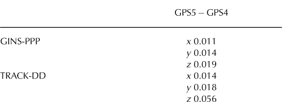
The root-mean-square (rms) value is used as an indication of the GPS noise level and remaining geophysical signals. Table 2 gives the rms values for Mertz Glacier sites GPS4, GPS5 and Penguin Point using the different processing strategies and software. The results are given in local topocentric coordinates (x, y, z) calculated over six stable days with 30 s sampling. For the ice sites GPS4 and GPS5, the coordinates are given on a tide-free signal.
Root-mean-square (rms) values (m) using different GPS processing techniques at rock and ice stations, processed in PPP with CSRS and GINS. The results are given in local topocentric coordinates (x, y, z) calculated over 6 days with 30 s sampling. For Mertz Glacier sites GPS4 and GPS5, the coordinates are given for a tide-free signal and on a detrended position
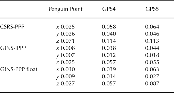
The rms values of the z components are substantially greater than those of the x and y components. This is mainly due to the ice sites recording more geophysical signal because of their movement. Different multipath character istics at the rock and ice sites will exist but likely only contribute a few millimeter of rms. We choose to calculate the rms over 6days in order to estimate the values for a 'stable' period, avoiding ionosphere spikes.
The results of the GPS processing strategies highlighted some clear findings. The highest rms value is on the vertical component, largely because of the geometry of the satellite constellation, unresolved tidal signals and other geophysical signals that are investigated below.
Comparing the GPS software (Table 2), we notice that the CSRS-PPP process allows the noise level to be reduced to ˜7cm for a rock station and 11 cm for an ice site. In comparison, the GINS-PPP software reduces these values to 2.5 cm for the rock sites and 5.5 cm for the ice sites. This implies that the residual ice signal is likely 3-4 cm rms.
The results from the GINS-PPP processing, using the float solution (PPP-float) and the ambiguities fixed to integer values (IPPP), are comparable in terms of noise level. However ambiguity fixing will have preferentially a larger impact on the spectrum of the time-series signal than on its rms value. Using the IPPP processing strategy drastically reduces the level of spurious signal seen, which frequently appears in high-frequency float PPP GPS time series (Reference Perosanz, Fund, Mercier, Loyer and CapdevillePerosanz and others, 2010).
In Table 3 we compare the rms values from the difference of the PPP solutions between GPS4 and GPS5 with ambiguities fixed to integers (called here GINS-PPP) and the results from a standard DD processing using TRACK. The TRACK command parameters set for the processing were mostly standard default setting and included ionosphere-free (LC) processing, an elevation cut-off angle of 10° and data noise levels of 3 mm for L1, L2 and 1 m for P1, P2. The MTT mapping function was used with a seasonal model (Reference Herring, Spoelstra and De MunckHerring, 1992). An IGS sp3 orbit file was used in the processing.
Root-mean-square (rms) values (m) using different processing techniques at the ice stations. The results are given in local topocentric coordinates (x, y, z) and over 6000 points (2 days with 30 s sampling). For the GINS-PPP solution, the values are given
for a tide-free detrended signal
We did not use Penguin Point as a base station, given its location far from the ice sites (˜47km away). The DD solution was processed with the shortest possible baseline (˜3 km) using GPS4 as the base station. This comparison allows us to evaluate the noise level of the GINS-PPP process. The DD solutions between GPS5 and GPS4 will difference common geophysical signal as PPP. The remain ing signal corresponds to the noise level and the non common geophysical signals.
Table 3 shows that rms values for the horizontal components are similar between TRACK-DD and GINS- PPP. For the vertical signal, the GINS-IPPP signal is up to 4cm better than TRACK-DD processing. The PPP process allows the rms of the time series to be comparable to (and in this case even better than) a standard but not optimized TRACK-DD processing solution.
Figure 3 shows the time series for GPS4, processed using GINS-IPPP, after removing a tidal signal. A cm-scale signal remains at periods of a few days. Part of this signal is explained by the effect of meteorological forcing on the ocean sea surface. To investigate this effect, we used TUGO (Toulouse Unstructured Grid Ocean), a barotropic non linear model with time integration derived from Reference Lynch and GrayLynch and Gray (1979), to model the oceanic response to barometric pressure and wind stress (Reference Le Bars, Lyard, Jeandel and DardengoLe Bars and others, 2010). Figure 3 indicates a good correlation of 0.89 between the de-tided height recorded by the GPS4 station and the sea surface height in response to atmospheric forcing (from 3 hour European Centre for Medium-Range Weather Forecasts (ECMWF) fields). Atmospheric forcing can explain 85% of the vertical signal at the few days scale period.
Comparison of GPS4 tide-free height (blue, processed with GINS-IPPP), ocean height from TUGO model (green) and their difference(red).

Table 4 summarizes the rms for the GPS5 vertical time series after removing different types of signal. The main component is the tide, which is responsible for >80% of the rms value. The response to the atmospheric forcing calcu lated from TUGO is responsible for ˜1 cm of the rms.
Characterization of the GPS5 height signal (m) (processed with GINS-PPP with ambiguities fixed to integer values) over 6 days: rms values

There still remains in the time series a component (<3 hour period) that is unmodeled by TUGO because of the 3 hour ECMWF sampling. Finally, bandpass filtering the GPS vertical time series between 5 and 30 min, we obtain an rms value of ˜1 cm, which is the maximum accuracy obtained for these data. In the next section, we investigate this bandpass-filtered signal in more detail.
Recording the Vibrations
The GPS stations on either side of the main rift recorded the GPS position of the glacier ice tongue every 30s. This relatively high-frequency sampling and the accuracy of the GINS-IPPP processing gives us access to ice-tongue signals at Nyquist periods of ˜1 min. Filtering the 60 day time series from the two GPS receivers with a bandpass filter (5–30 min in this example;see Fig. 4), we notice the presence of oscillations of the ice tongue detected by both GPS receivers.
Filtered signal of GPS4 height (light grey) and GPS5 height (black) between 5 and 30 min.

Both signals have much the same average amplitude (1-4 cm) and the same phase signal, but by comparing them with each other we notice a phase shift that changes with no consistent periodic behavior. These oscillating signals do not appear to be stationary in time, so we chose to use a wavelet transform technique that requires having a continuous periodic signal. This wavelet spectral technique has the advantage over traditional Fourier transforms for represent ing functions that have discontinuities and sharp peaks and for accurately deconstructing finite non-periodic time series. In our example (Fig. 5), we use a Morlet wavelet, which allows better time-frequency representation compared with the other wavelet selections (Reference Grinsted, Moore and JevrejevaGrinsted and others, 2004).
Wavelet transform of GPS4_TUGO height signal over 60 days: (a) time series of GPS4_TUGO; (b) wavelet transforms of GPS4_TUGO; (c) power spectrum of GPS4_TUGO.

With the wavelet representation of GPS4 height in Figure 5, we notice a first energetic signal peak between 5 and 30 min, a second between 60 and 120 min and a third between 240 and 390 min. The GPS harmonics periods are basically at the K1 tidal period and at its higher harmonics to the Nyquist level. These values do not correspond to the recorded energetic peaks.
The first peak between 5 and 30 min is the most remarkable. Its energy evolves in time, with non-periodic behavior and energy values ranging from 0 to 20 dB.
The two other signals have similar structures, with a modulation in time of their energy. This behavior suggests that this phenomenon is influenced by non-periodic external forcing. These signals are recorded in all three components of the GPS position, although only the height component is shown here.
In the first instance, we can imagine that the signals at ˜240min could be due to the effects of tides not modeled by the harmonic analysis. After analysis of the tide signal in the region, this tidal period shows amplitudes of a few millimeters, which is an order of magnitude smaller than the wavelet signal. Another possibility is from high-frequency tides of glaciological origin (Reference King, Makinson and GudmundssonKing and others, 2011).
Such kinds of periodic signal have been observed in the past. Reference Williams and RobinsonWilliams and Robinson (1981) described the pene tration of the ocean swell into the southern Ross Sea, Antarctica, where the ice cover is 300-600 m thick. As part of the Ross Ice Shelf Project (RISP;Reference Clough and HansenClough and Hansen, 1979), waves were observed during measurements of the ocean tide beneath the floating Ross Ice Shelf (Reference Williams and RobinsonWilliams and Robinson, 1981). Tide-recording gravimeters were used to monitor the elevation change at the surface of the ice shelf in response to the tide in the sub-adjacent water layer. The signals recorded were of two types: in addition to the tidal gravity changes, the gravimeters recorded a continuous motion containing periods shorter than 20 min. On the Ward Hunt Ice Shelf, Canada, three common oscillating strains were measured by strainmeter (Reference JeffriesJeffries, 1985): the first was at a 35-40 s period; the second was at a much longer period of ˜20 min; and the third was recorded at a 5.5-6.0 min period in Disraeli Fiord. Reference Thiel, Crary, Haubrich and BehrendtThiel and others (1960) reported observations of waves having periods shorter than 1 min. The waves recorded were flexural waves in a floating ice sheet, which are essentially fundamental mode Rayleigh waves on a solid that overlies a liquid (Reference Williams and RobinsonWilliams and Robinson, 1979).
In order to explain our observations in Figure 5, we calculated the fundamental vibration periods of the glacier ice tongue, considering flexural waves propagating on the ice tongue, modeled as an elastic beam, to look at the flexural waves going across a beam.
Origin Of Glacier Vibrations
Fundamental vibrations of the glacier ice tongue for the case of an Euler-Bernoulli beam: equations and boundary conditions
A causal link between natural oscillations of an ice tongue and iceberg calving has been suggested through the investigation of the Erebus Glacier tongue, Antarctica (Reference HoldsworthHoldsworth, 1969;Reference Goodman and HoldsworthGoodman and Holdsworth, 1978;Reference Holdsworth and GlynnHoldsworth and Glynn, 1981;Reference Vinogradov and HoldsworthVinogradov and Holdsworth, 1985;Reference Gui and SquireGui and Squire, 1989). The forcing mechanism from the ocean waves, passage of storms and atmospheric forcing provides energy at the natural modal frequencies of the ice tongue and induces its oscillations.
To calculate the fundamental vibrations of the glacier, we use an elastic-beam model, which is a simplification of the linear theory of elasticity for continuum solids (Euler- Bernoulli), to model the behavior of the ice flexure. The elastic approximation would be invalid if we were considering deformation of an ice tongue that was suffi ciently slow to allow the ice to creep. A summary of simplifications and assumptions is as follows (Reference Vinogradov and HoldsworthVinogradov and Holdsworth, 1985;Reference GudmundssonGudmundsson, 2007:
-
1. The glacier is treated as a uniform floating beam.
-
2. The motion of the beam is considered in two dimensions (2-D) only, namely in the vertical plane or the transverse plane. This simplification can be justified only if geometrically similar deformations take place across the width or in the vertical.
-
3. The beam material is assumed to behave elastically for all modes of deformation considered here. Viscous effects in the ice are neglected. Glen's flow law (Reference GlenGlen, 1955) is reserved for long-term viscous effects that underlie the static behavior of the ice shelf or floating body. The choice of an elastic relation is determined by the fact that ocean waves represent a high-frequency forcing.
-
4. The material properties are assumed to be constant throughout the beam. (We consider further below the case where the ice tongue consists of two parts separated by the rift.)
-
5. The effects of rotational inertia are neglected (taken into account in the Rayleigh model).
Although the ice-tongue profile shows a thickness approximately from 300 to 1200 m, the aspect ratio still corresponds to a thin ice beam.
In the Rayleigh model, the natural modes of free vibrations were calculated for a simplified ice-tongue geometry (Eqn (1)) and for three different types of boundary condition (Fig. 6):
Representation of boundary conditions in different configurations. (a) For a clamped beam and vibrations propagating in the alongflow direction, 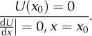 . (b) Then we consider the ice tongue as two beams separated by the rift in the middle. We obtain two beams, one clamped and the other on the front of the glacier and simply supported. For a clamped beam on the first part,
  (c) For a simply supported free-end beam on the second part,
  (d) The last case focuses on vibrations propagating in the across-flow direction. The beam is considered as a free–free end beam:


where u is the transverse displacement of the beam, EI is the stiffness per unit width, E is the elastic modulus, I is the inertia h3/12 and h the ice thickness, m is the beam mass per unit length and p(x,t) is the transverse loading on the beam due to water (where t is time). In this case we are not considering the tidal forcing (free vibrations), so p(x,t) = 0.
where U(x) is the amplitude of the vibrations and G(t) = G1 sin (ωt)G2cos(ωt). We replace u(x,t) in Eqn (1). The equation of the beam movement becomes

The solution of this equation is:

where ![]() is the wavenumber
is the wavenumber ![]() and p is the ice density.
and p is the ice density.
There are an infinite number of values that allow βn to be a solution of the system of equations. Each value corresponds to a vibration mode, but most of the movement can be described by the first few modes. Reference Robinson and HaskellRobinson and Haskell (1992) showed that the principal strain lies along the length of the tongue and the minor principal strain was found to be ˜-ã of the major principal strain which depends on ice-tongue configuration.
The natural frequencies are obtained from the wave number. This requires conditions to be imposed on the amplitude in the beam model (amplitude Eqn (4)), depend ing on configuration. The most usual boundary conditions set are those on the extremities of the beam. We consider three boundary conditions: clamped free end beam (Fig. 6a and b), simply supported free end beam (Fig. 6c) and fully floating beam (Fig. 6d), the tongue being assumed to float freely on the ocean.
Natural frequencies
In the rightmost column of Table 5, βn represents the wavenumber for the nth main mode of vibration of the beam and is multiplied by L (length of the beam) to give the non- dimensional wavenumber. We finally obtain
Non-dimensioned modal wavenumber β nL satisfying modal boundary conditions for the first, second and third modes

Tables 5 and 6 summarize the solutions of the model for the three main modes of vibrations for the different boundary conditions (Fig. 6a–d).
For each mode, the natural pulsation (and hence frequency) is given by

where L is the length (150, 75 or 30 km), b is the width (30 150 km) and h is the height, where h is the beam thickness (300–400 m).
Periods of Mertz Glacier ice–tongue vibrations (min) for several cases and for a constant height of 400m

In Figure 6, we use the dimensions of the ice tongue to calculate the solutions of Eqn (5) using the boundary conditions from Figure 6a–d.
The choice of elastic modulus deserves some discussion. Many studies using elastic deformation of ice relate to tidal bending. Whereas laboratory experiments show Young's modulus values in the range 8–10GPa (i.e. Reference LliboutryLliboutry, 1964; Reference Schulson and DuvalSchulson and Duval, 2009), Reference Holdsworth and HusseinyHoldsworth (1977) used a value of 2.7GPa and many studies since the 1990s have found 0.88GPa as a value better fitting tidal deformation observations (e.g. Reference VaughanVaughan, 1995). It can be argued in the case of tidal deformation that this deformation can be elastic, plastic or viscoelastic as suggested by Reed and others (2003). Reference Lingle, Hughes and KollmeyerLingle and others (1981) discuss the possibility that an equivalent thickness of the ice slab should be used given the state of fracture. Reference Rabus and LangRabus and Lang (2002) show that any model fitting needs to be done in 2–D to include the grounding–line curvature effects. Reference Legresy, Wendt, Tabacco, Remy and DietrichLegresy and others (2004) estimated the value of Efor Mertz Glacier by fitting the tidal deformation in straight grounding–line areas. They found a value of 0.88 GPa, compatible with the previous studies of Reference VaughanVaughan (1995). Another limitation of fitting tidal bending at the grounding line is that the shape of the ice tongue is far from being a straight beam (Reference Rabus and LangRabus and Lang, 2002). Propagation of elastic waves in the open–water section of Mertz Glacier ice tongue occurs in an almost flat rectangular section (compared with the grounding zone). The present study opens the possibility of testing the value of E since the vibrations we are looking at have much shorter periods (down to 5–30 min), where the deformation can be much better assumed as elastic than at the tidal periods. Hence we use E =9.33 GPa (Reference Schulson and DuvalSchulson and Duval, 2009) as the closest assumed value.
The resulting values of the ice–tongue vibration modes are shown in Figure 7 and seem to be organized into three different periods. The first, considering vibration going across the beam (L = 30 km), starts with the lowest values and with a main mode of ˜10min. The second (L =75 km) starts from 70 min and the last (L =150 km) has values from 287 min.
Variation of the fundamental vibrations of the ice tongue with the length and thickness for the second (a) and third modes (b), considering transverse vibrations and a fully floating ice tongue.

We are not looking at precise values of ice–tongue width, but rather at a representative set of values that could give us an idea of the frequencies expected. Moreover, we mainly focus on the second vibration mode, since the first mode is infinite or out of the representation of the wavelet transform and the following modes are less and less significant and with longer periods, where we would need to consider non elastic behaviors.
The frequencies are influenced by the dimensions taken into account in the calculations and the value of Young's modulus used.
In Table 5, note that the level of stress at the clamped end of the beam remains higher than the simply supported, fully floating case. In reality, the land/ice–tongue junction may not act exactly
as a clamp, but as a combination of a hinge and a clamp. As a result, the oscillation periods must be much lower at the flotation line. Furthermore, the effect of boundary conditions will tend to decrease from the flotation line to the free end and hence decrease the values of the periods and stresses.
Because the dimensions of the beam are not exact and can vary along its length in the real situation, we calculated (Fig. 7a and b) the frequencies of vibrations of the beam using a larger range of values. We focus in Figure 7 on vibrations going across the beam. We considered lengths ranging from 20 to 40 km (with steps of 5 km) and heights from 300 to 450 m (with steps of 25 m).
The period of fundamental vibration in this case goes from a few to 25 min for the second and third modes of vibration.
Considering the various dimensions of the beam (20–40 km length and 325–425 km thickness) we obtain vibration periods for the ice tongue of ˜10 min for the second mode, matching the first energetic peak seen in the wavelet analysis. The first energetic signal recorded from 5 to 30 min corresponds to the across–flow propagation of the vibrations, the second one to vibrations on each part of the broken ice tongue (separated by the rift) and the last one to the whole glacier tongue.
Finally, we focus on the influence of Young's modulus on the variation of periods and we obtain, for example, a value of ˜0.6 min GPa–1 for the second mode of the transverse case. However, varying the E coefficient in larger amounts leads to other vibration modes. Being more conclusive on 'determining' the best Ecoefficient with short–term vibration modes will require more in situ observations, including arrays of GPS, measurements of ocean forcing and eventually seismometer measurements of ice thickness, etc., in order not only to detect the vibrations, as done here, but also to see their propagation along the ice tongue.
These vibration mode values change with the height and the length of the beam but also with the value of Young's modulus. The components impacting most on this result are the length of the beam and Young's modulus. The length of the ice tongue will increase in time with the spreading flow of the glacier, and hence the mode of oscillation will change.
Origin of the Forcing
One of the main forcing mechanism candidates, which could explain the kind of forcing process observed above, is ocean swell, the effect of which on sea ice is easy to see. However the effect of ocean swell on the ice tongue has to take into account any sea–ice damping of the sea–swell energy (Reference Brunt, Okal and MacAyealBrunt and others, 2011). Satellite observations show no sea–ice cover a few kilometers around Mertz Glacier ice tongue during our 2 month observation period. The period of swell induced in this region is usually ˜10s. Such a short period is not recorded by our GPS, so we will need to set higher GPS sampling rates to obtain information about their impact on the ice tongue.
Reference Bromirski, Sergienko and MacAyealBromirski and others (2010) worked on one effect of infragravity (IG) waves on Antarctic ice shelves. They showed that long–period oceanic IG waves are generated by nonlinear wave interaction induced shoreward with moving storms. The effect of these longer waves induces a much higher–amplitude shelf response than ocean swell. IG waves could be a good candidate to produce and/or expand the pre–existing crevasses by a fatigue failure mechanism.
The periods measured in this latter case are 50–250s, which partly matches our GPS observations. Of course considering our 30s GPS sampling rate, we are not able to resolve signals with periods less than 1 min.
Discussion
In the previous section, we focused mainly on signals from a few minutes to a few hours. However, energetic signals may exist at periods less than 1 min or more than 10 hours, but the effect of these long–period signals is not considered in this study. Moreover we were not able to observe the higher– frequency signals due to the 30 s sampling period of our GPS records.
Both GPS4 and GPS5 sites recorded vibrations of the ice tongue, with the same energetic signals. To compare these signals, Figure 8 shows the differential signal between the two sites, separated by the main rift. First, we notice that our three energetic signals remain in the difference plot and have similar amplitudes. These remaining signals could be explained by both a differential amplitude between the GPS5 and GPS4 sites and/or a shift in phase between them. The two GPS stations have approximately the same amplitude but there is a phase shift between them. The phase shift causes a different response on the two parts of the ice tongue. The evolution of the phase shift between the two GPS sites suggests a mechanism constant in time and having the same phase difference values. This kind of movement could be associated with a torsional motion due to an oscillating force. Another possible reason for this movement is the different width and thickness of the two parts of the ice tongue in the area. With different width/thickness values, the fundamental vibration frequencies will not be exactly the same and this will make the two sides of the rift 'beat' with non–exact periods and hence a differential movement. In our simple model, the width/thickness values are calculated for a constant shelf length, but in reality the thickness profile changes significantly over time. Another factor, which could produce the same result, is associated with the increase in length of the glacier because of its flow. This would cause a change in the oscillation given the same forcing from waves.
Wavelet transform of GPS5–GPS4 height signal over 60 days: (a) time series of GPS5–GPS4; (b) wavelet transforms of GPS5–GPS4; (c) power spectrum of GPS5–GPS4.
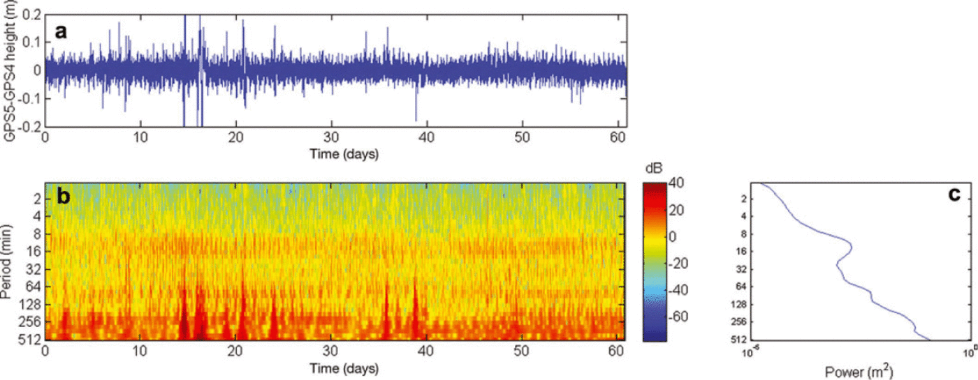
Fracture by fatigue failure occurs if a wave of sufficient amplitude acts for a long enough period of time. We showed that the rift opening is sensitive to wave frequencies and, as a result, a low fatigue failure can be induced in any beam depending on the incoming wave spectrum.
The rift is not assumed to be caused by this torsional movement, but this movement will increase the rift opening. The rift opening is known to be ˜12cmd–1, with a tide modulation of ±5cmd–1 (Reference LescarmontierLescarmontier, 2012). Ocean tidal currents influence the rift opening; westward currents tend to increase the rift opening (Reference LescarmontierLescarmontier, 2012). In addition, stresses producing fatigue failure may introduce a propagation of this rift. Finally, we must also consider the effect of refreezing occurring in the cracks which gives the rift the opportunity to recover after the previous history of cyclic loading. It would be interesting to investigate the time taken by the rift to open under a constant wave spectrum in comparison with the refreezing process to understand if this process could be sufficient by itself to open the rift.
To be able to fully understand this rifting process, we require more in situ GPS field data, especially for the across– flow direction of the glacier movement. We could then get a 2–D picture of the flexural mechanism and see at least the direction of propagation of the vibrations and wave forcing. Further observations are clearly needed to better character ize the amplitude, temporal variability and potential source areas of IG waves, in conjunction with glaciological modeling of ice–shelf–wave interaction.
Conclusions
During the CRAC–ICE missions of November 2007 and November 2009, we collected a range of data from ice– tongue and rock GPS stations in Antarctica.
The ice stations located on Mertz Glacier were analyzed using the selected high–performance GPS software GINS. Using a GINS–IPPP processing technique and wavelet analysis we were able to see clearly cm–scale signals usually hidden by the noise level of the GPS data.
Our comparisons with a simple elastic–beam model suggest that the GPS signals match some of the vibration modes of the ice tongue. The first vibration mode of ˜10 min corresponds to flexural wave propagation across the ice tongue. The last two modes, over 70 and 250min, likely correspond to waves propagating along the ice tongue. The vibrations propagating across the flow of the ice tongue are more evident due to the differential movement between the two parts of the ice tongue separated by the rift. This elastic model seems to be sufficient to explain the behavior of the ice tongue as an elastic beam. However, the introduction of plastic behavior may be useful as the next approach.
A range of periodic forcing mechanisms may contribute to the calving and disintegration of an ice tongue. The lower– period forcing terms are more likely to act on the across–flow vibrations, in contrast to the longer–period terms (tides) which will be more active on the along–flow vibrations.
Acknowledgements
This study is part of the CRAC–ICE project, supported by the CNES, ANR (Agence Nationale de la Recherche) DACOTA grant, IPEV, CNRS/INSU (Centre National de la Recherche Scientifique/Institut National des Sciences de l'Univers) and the University of Tasmania. We thank the GINS develop ment team and in particular Sylvain Loyer and Flavien Mercier for their help in using the software. We thank Pascal Lacroix who participated in the early development of the project and in the deployment of the GPS stations, the data from which are used in this study. We thank Tom Herring for the TRACK processing.


