


1. Introduction
Researchers in the field of network psychometrics (Marsman et al., Reference Marsman, Borsboom, Kruis, Epskamp, van Bork, Waldorp and Marsman2018) study the estimation of multivariate statistical models in attempts to map out the complex interplay of interactions between variables. This field emerged from the network perspective on psychology (Borsboom, Reference Borsboom2017; Cramer, Waldorp, van der Maas, & Borsboom, Reference Cramer, Waldorp, van der Maas and Borsboom2010)—departing from the latent variable model and instead conceptualizing observed variables (e.g., attitudes, symptoms, and moods) as causal agents in a complex interplay of psychological (and other) components. In recent years, network models have become useful additions to the psychometric toolbox. For example, network models provide useful visualization tools to check the fit of latent variable models (Epskamp, Cramer, Waldrop, Schmittmann, & Borsboom, Reference Epskamp, Cramer, Waldrop, Schmittmann and Borsboom2012), are closely tied and often equivalent to latent variable models (Marsman et al., Reference Marsman, Borsboom, Kruis, Epskamp, van Bork, Waldorp and Marsman2018), are often uniquely identified (Epskamp, Waldorp, Mõttus, & Borsboom, Reference Epskamp, Waldorp, Mõttus and Borsboom2018), and may provide exploratory insight into the underlying factor structure by investigating its clustering (Golino & Epskamp, Reference Golino and Epskamp2017).
In a psychometric network model,Footnote 1 variables are represented by nodes that are connected by edges, which are weighted according to some statistic. In this paper, I focus on two particular network models now routinely used in the analysis of continuous data: the Gaussian graphical model (GGM; Epskamp, Waldorp, et al., Reference Epskamp, Waldorp, Mõttus and Borsboom2018; Lauritzen, Reference Lauritzen1996) and the graphical vector-autoregression model (GVAR; Epskamp, Waldorp, et al., Reference Epskamp, Waldorp, Mõttus and Borsboom2018; Wild et al., Reference Wild, Eichler, Friederich, Hartmann, Zipfel and Herzog2010). The GGM forms an undirected network model, in which edges represent partial correlation coefficients. The GGM is closely tied, but not fully equivalent, to the directed structures typically used in structural equation modeling (SEM; Epskamp, Rhemtulla, & Borsboom, Reference Epskamp, Rhemtulla and Borsboom2017) and is often estimated from cross-sectional data (Fried et al., Reference Fried, van Borkulo, Cramer, Boschloo, Schoevers and Borsboom2017), in which many subjects are measured only once. The (lag-1) GVAR model takes the form of a generalization of the GGM in single-subject time series (Epskamp, Waldorp, et al., Reference Epskamp, Waldorp, Mõttus and Borsboom2018). In the GVAR, temporal dependencies are modeled via a regression on the previous measurement occasion, which leads to a matrix of regression coefficients that can also be used to draw a directed network model (Bringmann et al., Reference Bringmann, Vissers, Wichers, Geschwind, Kuppens, Peeters and Tuerlinckx2013)—often termed the temporal network because it encodes predictive effects over time. The remaining variances and covariances (i.e., the covariance structure after controlling for the previous measurement occasion) can be modeled as a GGM, which is also termed the contemporaneous network. When time series of multiple subjects are available, a third GGM can be formed on the between-subject effects (relationships between stable means)—also termed the between-subject network.
Current practices in network psychometrics feature two pressing limitations. (1) Although network modeling has been proposed as an alternative to latent variable modeling (i.e., covariation is caused by one or more unobserved common causes), the complete omission of latent variables may be one step too far (Bringmann & Eronen, Reference Bringmann and Eronen2018; Fried & Cramer, Reference Fried and Cramer2017; Guyon, Falissard, & Kop, Reference Guyon, Falissard and Kop2017). Network models for observed variables rely on the assumption that all causally interacting variables are observed without error. However, a certain level of measurement error (Schuurman, Houtveen, & Hamaker, Reference Schuurman, Houtveen and Hamaker2015) should be assumed in psychological data. (2) Network models are now often estimated from cross-sectional data. However, such results are not reflective of within-subject dynamics over time (Bos et al., Reference Bos, Snippe, de Vos, Hartmann, Simons, van der Krieke and Wichers2017; Molenaar, Reference Molenaar2004). Cross-sectional analysis cannot distinguish between within- and between-subject variances (Hamaker, Reference Hamaker, Mehl and Conner2012) or indeed investigate temporal effects over time. In principle, panel data, in which many subjects are measured a few times, can be used to distinguish between within- and between-subject effects (Hamaker, Kuiper, & Grasman, Reference Hamaker, Kuiper and Grasman2015), but have only been sparingly discussed in network psychometrics (e.g., Rhemtulla, Van Bork, & Cramer, Reference Rhemtulla, Van Bork and Cramer2017). Prior literature has tackled these topics separately. For example, Epskamp, Rhemtulla, and Borsboom (Reference Epskamp, Rhemtulla and Borsboom2017) addressed Limitation 1 by proposing to form a psychometric framework to incorporate GGMs in latent variable models, both at the latent level (latent network models) and at the residual level (residual network models). The multi-level GVAR model (Epskamp, Waldorp, et al., Reference Epskamp, Waldorp, Mõttus and Borsboom2018) can overcome Limitation 2 but does not include latent variables and requires intensive repeated measures of many subjects.
The goal in this paper is to combine the above-described solutions into a general framework. The framework emerges by combining a general factor model and a GVAR model and is referred to as the lvgvar model.Footnote 2 I will discuss estimation in two very distinct settings:
-
• Time-series data of a single subject. This setting will be termed ts-lvgvar.
-
• Panel data of many subjects measured on a few (at least three) measurement occasions. This setting will be termed panel-lvgvar.
These settings differ crucially from one another. ts-lvgvar concerns a fixed subject (fixed subject p), which involves variation over measurement occasions (random time T). Meanwhile, panel-lvgvar concerns variation over subjects (random subject P) at a few fixed time points
\documentclass[12pt]{minimal}
\usepackage{amsmath}
\usepackage{wasysym}
\usepackage{amsfonts}
\usepackage{amssymb}
\usepackage{amsbsy}
\usepackage{mathrsfs}
\usepackage{upgreek}
\setlength{\oddsidemargin}{-69pt}
\begin{document}$$t, t+1, t+2, \ldots $$\end{document}
 . The panel-lvgvar is a multi-level model with random effects on the mean structure. I showcase both methods using two empirical examples and assess the performance of model search strategies through two large-scale simulation studies. Finally, I discuss the generalizability of results between these settings in detail. The lvgvar framework is implemented in the open-source software package psychonetrics.Footnote 3
2. Preliminary Topics
2.1. Notation
This paper uses a similar notation as Epskamp, Waldorp, et al.
(Reference Epskamp, Waldorp, Mõttus and Borsboom2018). Roman letters indicate observed variables, and Greek letters indicate parameters or latent variables. Bold-faced lowercase letters indicate vectors, and bold-faced uppercase letters indicate matrices. Normal-faced lowercase letters indicate fixed values, and normal-faced uppercase letters indicate random variables. These notations are also used in the subscript of a vector. For example,
\documentclass[12pt]{minimal}
\usepackage{amsmath}
\usepackage{wasysym}
\usepackage{amsfonts}
\usepackage{amssymb}
\usepackage{amsbsy}
\usepackage{mathrsfs}
\usepackage{upgreek}
\setlength{\oddsidemargin}{-69pt}
\begin{document}$$\pmb {y}_{p,t}$$\end{document}
 indicates a fixed response pattern
\documentclass[12pt]{minimal}
\usepackage{amsmath}
\usepackage{wasysym}
\usepackage{amsfonts}
\usepackage{amssymb}
\usepackage{amsbsy}
\usepackage{mathrsfs}
\usepackage{upgreek}
\setlength{\oddsidemargin}{-69pt}
\begin{document}$$\pmb {y}$$\end{document}
indicates a fixed response pattern
\documentclass[12pt]{minimal}
\usepackage{amsmath}
\usepackage{wasysym}
\usepackage{amsfonts}
\usepackage{amssymb}
\usepackage{amsbsy}
\usepackage{mathrsfs}
\usepackage{upgreek}
\setlength{\oddsidemargin}{-69pt}
\begin{document}$$\pmb {y}$$\end{document}
 for subject p on fixed measurement occasion t;
\documentclass[12pt]{minimal}
\usepackage{amsmath}
\usepackage{wasysym}
\usepackage{amsfonts}
\usepackage{amssymb}
\usepackage{amsbsy}
\usepackage{mathrsfs}
\usepackage{upgreek}
\setlength{\oddsidemargin}{-69pt}
\begin{document}$$\pmb {y}_{P,t}$$\end{document}
for subject p on fixed measurement occasion t;
\documentclass[12pt]{minimal}
\usepackage{amsmath}
\usepackage{wasysym}
\usepackage{amsfonts}
\usepackage{amssymb}
\usepackage{amsbsy}
\usepackage{mathrsfs}
\usepackage{upgreek}
\setlength{\oddsidemargin}{-69pt}
\begin{document}$$\pmb {y}_{P,t}$$\end{document}
 indicates the response vector of a random subject P at fixed measurement occasion t; and
\documentclass[12pt]{minimal}
\usepackage{amsmath}
\usepackage{wasysym}
\usepackage{amsfonts}
\usepackage{amssymb}
\usepackage{amsbsy}
\usepackage{mathrsfs}
\usepackage{upgreek}
\setlength{\oddsidemargin}{-69pt}
\begin{document}$$\pmb {y}_{p,T}$$\end{document}
indicates the response vector of a random subject P at fixed measurement occasion t; and
\documentclass[12pt]{minimal}
\usepackage{amsmath}
\usepackage{wasysym}
\usepackage{amsfonts}
\usepackage{amssymb}
\usepackage{amsbsy}
\usepackage{mathrsfs}
\usepackage{upgreek}
\setlength{\oddsidemargin}{-69pt}
\begin{document}$$\pmb {y}_{p,T}$$\end{document}
 indicates the response vector of a fixed subject p at a random measurement occasion T.
2.2. Estimation
Suppose n cases (people or time points in this paper) are measured on
\documentclass[12pt]{minimal}
\usepackage{amsmath}
\usepackage{wasysym}
\usepackage{amsfonts}
\usepackage{amssymb}
\usepackage{amsbsy}
\usepackage{mathrsfs}
\usepackage{upgreek}
\setlength{\oddsidemargin}{-69pt}
\begin{document}$$n_z$$\end{document}
 variables, with
\documentclass[12pt]{minimal}
\usepackage{amsmath}
\usepackage{wasysym}
\usepackage{amsfonts}
\usepackage{amssymb}
\usepackage{amsbsy}
\usepackage{mathrsfs}
\usepackage{upgreek}
\setlength{\oddsidemargin}{-69pt}
\begin{document}$$\pmb {z}_c$$\end{document}
variables, with
\documentclass[12pt]{minimal}
\usepackage{amsmath}
\usepackage{wasysym}
\usepackage{amsfonts}
\usepackage{amssymb}
\usepackage{amsbsy}
\usepackage{mathrsfs}
\usepackage{upgreek}
\setlength{\oddsidemargin}{-69pt}
\begin{document}$$\pmb {z}_c$$\end{document}
 denoting the response vector of case c, which is the cth row of a data matrix
\documentclass[12pt]{minimal}
\usepackage{amsmath}
\usepackage{wasysym}
\usepackage{amsfonts}
\usepackage{amssymb}
\usepackage{amsbsy}
\usepackage{mathrsfs}
\usepackage{upgreek}
\setlength{\oddsidemargin}{-69pt}
\begin{document}$$\pmb {Z}$$\end{document}
denoting the response vector of case c, which is the cth row of a data matrix
\documentclass[12pt]{minimal}
\usepackage{amsmath}
\usepackage{wasysym}
\usepackage{amsfonts}
\usepackage{amssymb}
\usepackage{amsbsy}
\usepackage{mathrsfs}
\usepackage{upgreek}
\setlength{\oddsidemargin}{-69pt}
\begin{document}$$\pmb {Z}$$\end{document}
 . The vector
\documentclass[12pt]{minimal}
\usepackage{amsmath}
\usepackage{wasysym}
\usepackage{amsfonts}
\usepackage{amssymb}
\usepackage{amsbsy}
\usepackage{mathrsfs}
\usepackage{upgreek}
\setlength{\oddsidemargin}{-69pt}
\begin{document}$$\pmb {z}_C$$\end{document}
. The vector
\documentclass[12pt]{minimal}
\usepackage{amsmath}
\usepackage{wasysym}
\usepackage{amsfonts}
\usepackage{amssymb}
\usepackage{amsbsy}
\usepackage{mathrsfs}
\usepackage{upgreek}
\setlength{\oddsidemargin}{-69pt}
\begin{document}$$\pmb {z}_C$$\end{document}
 will be assumed normally distributed:

in which
\documentclass[12pt]{minimal}
\usepackage{amsmath}
\usepackage{wasysym}
\usepackage{amsfonts}
\usepackage{amssymb}
\usepackage{amsbsy}
\usepackage{mathrsfs}
\usepackage{upgreek}
\setlength{\oddsidemargin}{-69pt}
\begin{document}$$\pmb {\mu }$$\end{document}
 represents a mean vector and
\documentclass[12pt]{minimal}
\usepackage{amsmath}
\usepackage{wasysym}
\usepackage{amsfonts}
\usepackage{amssymb}
\usepackage{amsbsy}
\usepackage{mathrsfs}
\usepackage{upgreek}
\setlength{\oddsidemargin}{-69pt}
\begin{document}$$\pmb {\Sigma }$$\end{document}
represents a mean vector and
\documentclass[12pt]{minimal}
\usepackage{amsmath}
\usepackage{wasysym}
\usepackage{amsfonts}
\usepackage{amssymb}
\usepackage{amsbsy}
\usepackage{mathrsfs}
\usepackage{upgreek}
\setlength{\oddsidemargin}{-69pt}
\begin{document}$$\pmb {\Sigma }$$\end{document}
 represents a variance–covariance matrix.Footnote 4 Let
\documentclass[12pt]{minimal}
\usepackage{amsmath}
\usepackage{wasysym}
\usepackage{amsfonts}
\usepackage{amssymb}
\usepackage{amsbsy}
\usepackage{mathrsfs}
\usepackage{upgreek}
\setlength{\oddsidemargin}{-69pt}
\begin{document}$$\bar{\pmb {z}}$$\end{document}
represents a variance–covariance matrix.Footnote 4 Let
\documentclass[12pt]{minimal}
\usepackage{amsmath}
\usepackage{wasysym}
\usepackage{amsfonts}
\usepackage{amssymb}
\usepackage{amsbsy}
\usepackage{mathrsfs}
\usepackage{upgreek}
\setlength{\oddsidemargin}{-69pt}
\begin{document}$$\bar{\pmb {z}}$$\end{document}
 represent the sample means:

Furthermore, let
\documentclass[12pt]{minimal}
\usepackage{amsmath}
\usepackage{wasysym}
\usepackage{amsfonts}
\usepackage{amssymb}
\usepackage{amsbsy}
\usepackage{mathrsfs}
\usepackage{upgreek}
\setlength{\oddsidemargin}{-69pt}
\begin{document}$$\bar{\pmb {S}}$$\end{document}
 represent the sample variance–covariance matrix:

Using these summary statistics and assuming multivariate normality, we can estimate parameters by minimizing the following fit function:

which is proportional to
\documentclass[12pt]{minimal}
\usepackage{amsmath}
\usepackage{wasysym}
\usepackage{amsfonts}
\usepackage{amssymb}
\usepackage{amsbsy}
\usepackage{mathrsfs}
\usepackage{upgreek}
\setlength{\oddsidemargin}{-69pt}
\begin{document}$$-2/n$$\end{document}
 times the log-likelihood of the data. Full information maximum likelihood estimation (FIML) can be used when data are missing. To this end, the data can be subdivided in subsets of data that have the same missingness patterns. The FIML fit function to be minimized takes the following form:

in which
\documentclass[12pt]{minimal}
\usepackage{amsmath}
\usepackage{wasysym}
\usepackage{amsfonts}
\usepackage{amssymb}
\usepackage{amsbsy}
\usepackage{mathrsfs}
\usepackage{upgreek}
\setlength{\oddsidemargin}{-69pt}
\begin{document}$$n_i$$\end{document}
 represents the sample size of subset i;
\documentclass[12pt]{minimal}
\usepackage{amsmath}
\usepackage{wasysym}
\usepackage{amsfonts}
\usepackage{amssymb}
\usepackage{amsbsy}
\usepackage{mathrsfs}
\usepackage{upgreek}
\setlength{\oddsidemargin}{-69pt}
\begin{document}$$\pmb {S}_i$$\end{document}
represents the sample size of subset i;
\documentclass[12pt]{minimal}
\usepackage{amsmath}
\usepackage{wasysym}
\usepackage{amsfonts}
\usepackage{amssymb}
\usepackage{amsbsy}
\usepackage{mathrsfs}
\usepackage{upgreek}
\setlength{\oddsidemargin}{-69pt}
\begin{document}$$\pmb {S}_i$$\end{document}
 is the sample variance–covariance matrix of subset i (note,
\documentclass[12pt]{minimal}
\usepackage{amsmath}
\usepackage{wasysym}
\usepackage{amsfonts}
\usepackage{amssymb}
\usepackage{amsbsy}
\usepackage{mathrsfs}
\usepackage{upgreek}
\setlength{\oddsidemargin}{-69pt}
\begin{document}$$\pmb {S}_i = \pmb {O}$$\end{document}
is the sample variance–covariance matrix of subset i (note,
\documentclass[12pt]{minimal}
\usepackage{amsmath}
\usepackage{wasysym}
\usepackage{amsfonts}
\usepackage{amssymb}
\usepackage{amsbsy}
\usepackage{mathrsfs}
\usepackage{upgreek}
\setlength{\oddsidemargin}{-69pt}
\begin{document}$$\pmb {S}_i = \pmb {O}$$\end{document}
 if
\documentclass[12pt]{minimal}
\usepackage{amsmath}
\usepackage{wasysym}
\usepackage{amsfonts}
\usepackage{amssymb}
\usepackage{amsbsy}
\usepackage{mathrsfs}
\usepackage{upgreek}
\setlength{\oddsidemargin}{-69pt}
\begin{document}$$n_i = 1$$\end{document}
if
\documentclass[12pt]{minimal}
\usepackage{amsmath}
\usepackage{wasysym}
\usepackage{amsfonts}
\usepackage{amssymb}
\usepackage{amsbsy}
\usepackage{mathrsfs}
\usepackage{upgreek}
\setlength{\oddsidemargin}{-69pt}
\begin{document}$$n_i = 1$$\end{document}
 );
\documentclass[12pt]{minimal}
\usepackage{amsmath}
\usepackage{wasysym}
\usepackage{amsfonts}
\usepackage{amssymb}
\usepackage{amsbsy}
\usepackage{mathrsfs}
\usepackage{upgreek}
\setlength{\oddsidemargin}{-69pt}
\begin{document}$$\bar{\pmb {z}_i}$$\end{document}
);
\documentclass[12pt]{minimal}
\usepackage{amsmath}
\usepackage{wasysym}
\usepackage{amsfonts}
\usepackage{amssymb}
\usepackage{amsbsy}
\usepackage{mathrsfs}
\usepackage{upgreek}
\setlength{\oddsidemargin}{-69pt}
\begin{document}$$\bar{\pmb {z}_i}$$\end{document}
 conotes the sample means of subset i (note, it is the same as the observed score if
\documentclass[12pt]{minimal}
\usepackage{amsmath}
\usepackage{wasysym}
\usepackage{amsfonts}
\usepackage{amssymb}
\usepackage{amsbsy}
\usepackage{mathrsfs}
\usepackage{upgreek}
\setlength{\oddsidemargin}{-69pt}
\begin{document}$$n_i = 1$$\end{document}
conotes the sample means of subset i (note, it is the same as the observed score if
\documentclass[12pt]{minimal}
\usepackage{amsmath}
\usepackage{wasysym}
\usepackage{amsfonts}
\usepackage{amssymb}
\usepackage{amsbsy}
\usepackage{mathrsfs}
\usepackage{upgreek}
\setlength{\oddsidemargin}{-69pt}
\begin{document}$$n_i = 1$$\end{document}
 );
\documentclass[12pt]{minimal}
\usepackage{amsmath}
\usepackage{wasysym}
\usepackage{amsfonts}
\usepackage{amssymb}
\usepackage{amsbsy}
\usepackage{mathrsfs}
\usepackage{upgreek}
\setlength{\oddsidemargin}{-69pt}
\begin{document}$$\pmb {\Sigma }_i$$\end{document}
);
\documentclass[12pt]{minimal}
\usepackage{amsmath}
\usepackage{wasysym}
\usepackage{amsfonts}
\usepackage{amssymb}
\usepackage{amsbsy}
\usepackage{mathrsfs}
\usepackage{upgreek}
\setlength{\oddsidemargin}{-69pt}
\begin{document}$$\pmb {\Sigma }_i$$\end{document}
 is a subset of
\documentclass[12pt]{minimal}
\usepackage{amsmath}
\usepackage{wasysym}
\usepackage{amsfonts}
\usepackage{amssymb}
\usepackage{amsbsy}
\usepackage{mathrsfs}
\usepackage{upgreek}
\setlength{\oddsidemargin}{-69pt}
\begin{document}$$\pmb {\Sigma }$$\end{document}
is a subset of
\documentclass[12pt]{minimal}
\usepackage{amsmath}
\usepackage{wasysym}
\usepackage{amsfonts}
\usepackage{amssymb}
\usepackage{amsbsy}
\usepackage{mathrsfs}
\usepackage{upgreek}
\setlength{\oddsidemargin}{-69pt}
\begin{document}$$\pmb {\Sigma }$$\end{document}
 that only contains elements of observed data in subset i; and
\documentclass[12pt]{minimal}
\usepackage{amsmath}
\usepackage{wasysym}
\usepackage{amsfonts}
\usepackage{amssymb}
\usepackage{amsbsy}
\usepackage{mathrsfs}
\usepackage{upgreek}
\setlength{\oddsidemargin}{-69pt}
\begin{document}$$\pmb {\mu }_i$$\end{document}
that only contains elements of observed data in subset i; and
\documentclass[12pt]{minimal}
\usepackage{amsmath}
\usepackage{wasysym}
\usepackage{amsfonts}
\usepackage{amssymb}
\usepackage{amsbsy}
\usepackage{mathrsfs}
\usepackage{upgreek}
\setlength{\oddsidemargin}{-69pt}
\begin{document}$$\pmb {\mu }_i$$\end{document}
 is a subset of
\documentclass[12pt]{minimal}
\usepackage{amsmath}
\usepackage{wasysym}
\usepackage{amsfonts}
\usepackage{amssymb}
\usepackage{amsbsy}
\usepackage{mathrsfs}
\usepackage{upgreek}
\setlength{\oddsidemargin}{-69pt}
\begin{document}$$\pmb {\mu }$$\end{document}
is a subset of
\documentclass[12pt]{minimal}
\usepackage{amsmath}
\usepackage{wasysym}
\usepackage{amsfonts}
\usepackage{amssymb}
\usepackage{amsbsy}
\usepackage{mathrsfs}
\usepackage{upgreek}
\setlength{\oddsidemargin}{-69pt}
\begin{document}$$\pmb {\mu }$$\end{document}
 that only contains elements of observed data in subset i.
2.3. Factor Model
Let
\documentclass[12pt]{minimal}
\usepackage{amsmath}
\usepackage{wasysym}
\usepackage{amsfonts}
\usepackage{amssymb}
\usepackage{amsbsy}
\usepackage{mathrsfs}
\usepackage{upgreek}
\setlength{\oddsidemargin}{-69pt}
\begin{document}$$\pmb {\eta }_{p,t}$$\end{document}
 indicate a length
\documentclass[12pt]{minimal}
\usepackage{amsmath}
\usepackage{wasysym}
\usepackage{amsfonts}
\usepackage{amssymb}
\usepackage{amsbsy}
\usepackage{mathrsfs}
\usepackage{upgreek}
\setlength{\oddsidemargin}{-69pt}
\begin{document}$$n_\eta $$\end{document}
indicate a length
\documentclass[12pt]{minimal}
\usepackage{amsmath}
\usepackage{wasysym}
\usepackage{amsfonts}
\usepackage{amssymb}
\usepackage{amsbsy}
\usepackage{mathrsfs}
\usepackage{upgreek}
\setlength{\oddsidemargin}{-69pt}
\begin{document}$$n_\eta $$\end{document}
 vector of variables of interest at time point t for subject p. If
\documentclass[12pt]{minimal}
\usepackage{amsmath}
\usepackage{wasysym}
\usepackage{amsfonts}
\usepackage{amssymb}
\usepackage{amsbsy}
\usepackage{mathrsfs}
\usepackage{upgreek}
\setlength{\oddsidemargin}{-69pt}
\begin{document}$$\pmb {\eta }$$\end{document}
vector of variables of interest at time point t for subject p. If
\documentclass[12pt]{minimal}
\usepackage{amsmath}
\usepackage{wasysym}
\usepackage{amsfonts}
\usepackage{amssymb}
\usepackage{amsbsy}
\usepackage{mathrsfs}
\usepackage{upgreek}
\setlength{\oddsidemargin}{-69pt}
\begin{document}$$\pmb {\eta }$$\end{document}
 is not observed, it may be assumed that
\documentclass[12pt]{minimal}
\usepackage{amsmath}
\usepackage{wasysym}
\usepackage{amsfonts}
\usepackage{amssymb}
\usepackage{amsbsy}
\usepackage{mathrsfs}
\usepackage{upgreek}
\setlength{\oddsidemargin}{-69pt}
\begin{document}$$\pmb {\eta }$$\end{document}
is not observed, it may be assumed that
\documentclass[12pt]{minimal}
\usepackage{amsmath}
\usepackage{wasysym}
\usepackage{amsfonts}
\usepackage{amssymb}
\usepackage{amsbsy}
\usepackage{mathrsfs}
\usepackage{upgreek}
\setlength{\oddsidemargin}{-69pt}
\begin{document}$$\pmb {\eta }$$\end{document}
 linearly causes observed indicators in a length
\documentclass[12pt]{minimal}
\usepackage{amsmath}
\usepackage{wasysym}
\usepackage{amsfonts}
\usepackage{amssymb}
\usepackage{amsbsy}
\usepackage{mathrsfs}
\usepackage{upgreek}
\setlength{\oddsidemargin}{-69pt}
\begin{document}$$n_y$$\end{document}
linearly causes observed indicators in a length
\documentclass[12pt]{minimal}
\usepackage{amsmath}
\usepackage{wasysym}
\usepackage{amsfonts}
\usepackage{amssymb}
\usepackage{amsbsy}
\usepackage{mathrsfs}
\usepackage{upgreek}
\setlength{\oddsidemargin}{-69pt}
\begin{document}$$n_y$$\end{document}
 vector
\documentclass[12pt]{minimal}
\usepackage{amsmath}
\usepackage{wasysym}
\usepackage{amsfonts}
\usepackage{amssymb}
\usepackage{amsbsy}
\usepackage{mathrsfs}
\usepackage{upgreek}
\setlength{\oddsidemargin}{-69pt}
\begin{document}$$\pmb {y}$$\end{document}
vector
\documentclass[12pt]{minimal}
\usepackage{amsmath}
\usepackage{wasysym}
\usepackage{amsfonts}
\usepackage{amssymb}
\usepackage{amsbsy}
\usepackage{mathrsfs}
\usepackage{upgreek}
\setlength{\oddsidemargin}{-69pt}
\begin{document}$$\pmb {y}$$\end{document}
 according to a linear factor model:

in which
\documentclass[12pt]{minimal}
\usepackage{amsmath}
\usepackage{wasysym}
\usepackage{amsfonts}
\usepackage{amssymb}
\usepackage{amsbsy}
\usepackage{mathrsfs}
\usepackage{upgreek}
\setlength{\oddsidemargin}{-69pt}
\begin{document}$$\pmb {\tau }$$\end{document}
 is a general intercept vector;
\documentclass[12pt]{minimal}
\usepackage{amsmath}
\usepackage{wasysym}
\usepackage{amsfonts}
\usepackage{amssymb}
\usepackage{amsbsy}
\usepackage{mathrsfs}
\usepackage{upgreek}
\setlength{\oddsidemargin}{-69pt}
\begin{document}$$\pmb {\Lambda }$$\end{document}
is a general intercept vector;
\documentclass[12pt]{minimal}
\usepackage{amsmath}
\usepackage{wasysym}
\usepackage{amsfonts}
\usepackage{amssymb}
\usepackage{amsbsy}
\usepackage{mathrsfs}
\usepackage{upgreek}
\setlength{\oddsidemargin}{-69pt}
\begin{document}$$\pmb {\Lambda }$$\end{document}
 is a matrix of factor loadings; and
\documentclass[12pt]{minimal}
\usepackage{amsmath}
\usepackage{wasysym}
\usepackage{amsfonts}
\usepackage{amssymb}
\usepackage{amsbsy}
\usepackage{mathrsfs}
\usepackage{upgreek}
\setlength{\oddsidemargin}{-69pt}
\begin{document}$$\pmb {\varepsilon }_{p,t}$$\end{document}
is a matrix of factor loadings; and
\documentclass[12pt]{minimal}
\usepackage{amsmath}
\usepackage{wasysym}
\usepackage{amsfonts}
\usepackage{amssymb}
\usepackage{amsbsy}
\usepackage{mathrsfs}
\usepackage{upgreek}
\setlength{\oddsidemargin}{-69pt}
\begin{document}$$\pmb {\varepsilon }_{p,t}$$\end{document}
 is a vector of residuals. Assume that the residuals, denoting measurement error or nuisance variables, have mean
\documentclass[12pt]{minimal}
\usepackage{amsmath}
\usepackage{wasysym}
\usepackage{amsfonts}
\usepackage{amssymb}
\usepackage{amsbsy}
\usepackage{mathrsfs}
\usepackage{upgreek}
\setlength{\oddsidemargin}{-69pt}
\begin{document}$$\pmb {0}$$\end{document}
is a vector of residuals. Assume that the residuals, denoting measurement error or nuisance variables, have mean
\documentclass[12pt]{minimal}
\usepackage{amsmath}
\usepackage{wasysym}
\usepackage{amsfonts}
\usepackage{amssymb}
\usepackage{amsbsy}
\usepackage{mathrsfs}
\usepackage{upgreek}
\setlength{\oddsidemargin}{-69pt}
\begin{document}$$\pmb {0}$$\end{document}
 across people but not necessarily across time:

It is possible, without loss of information, to regard any of the above variable vectors as composites of the mean of subject p, denoted with
\documentclass[12pt]{minimal}
\usepackage{amsmath}
\usepackage{wasysym}
\usepackage{amsfonts}
\usepackage{amssymb}
\usepackage{amsbsy}
\usepackage{mathrsfs}
\usepackage{upgreek}
\setlength{\oddsidemargin}{-69pt}
\begin{document}$$\pmb {\mu }_p$$\end{document}
 , and deviation from that mean in measurement t, denoted with
\documentclass[12pt]{minimal}
\usepackage{amsmath}
\usepackage{wasysym}
\usepackage{amsfonts}
\usepackage{amssymb}
\usepackage{amsbsy}
\usepackage{mathrsfs}
\usepackage{upgreek}
\setlength{\oddsidemargin}{-69pt}
\begin{document}$$\pmb {\xi }_{p,t}$$\end{document}
, and deviation from that mean in measurement t, denoted with
\documentclass[12pt]{minimal}
\usepackage{amsmath}
\usepackage{wasysym}
\usepackage{amsfonts}
\usepackage{amssymb}
\usepackage{amsbsy}
\usepackage{mathrsfs}
\usepackage{upgreek}
\setlength{\oddsidemargin}{-69pt}
\begin{document}$$\pmb {\xi }_{p,t}$$\end{document}
 :
:

with the expected value of all
\documentclass[12pt]{minimal}
\usepackage{amsmath}
\usepackage{wasysym}
\usepackage{amsfonts}
\usepackage{amssymb}
\usepackage{amsbsy}
\usepackage{mathrsfs}
\usepackage{upgreek}
\setlength{\oddsidemargin}{-69pt}
\begin{document}$$\pmb {\xi }$$\end{document}
 vectors concerning either random people or random measurement occasions set to equal zero and no assumed temporal dependency between the residual deviations. It is then possible to formulate the measurement model of Eq. (3) in a within-subject and a between-subject part:

Note, the lack of subscripts on
\documentclass[12pt]{minimal}
\usepackage{amsmath}
\usepackage{wasysym}
\usepackage{amsfonts}
\usepackage{amssymb}
\usepackage{amsbsy}
\usepackage{mathrsfs}
\usepackage{upgreek}
\setlength{\oddsidemargin}{-69pt}
\begin{document}$$\pmb {\Lambda }$$\end{document}
 and
\documentclass[12pt]{minimal}
\usepackage{amsmath}
\usepackage{wasysym}
\usepackage{amsfonts}
\usepackage{amssymb}
\usepackage{amsbsy}
\usepackage{mathrsfs}
\usepackage{upgreek}
\setlength{\oddsidemargin}{-69pt}
\begin{document}$$\pmb {\tau }$$\end{document}
and
\documentclass[12pt]{minimal}
\usepackage{amsmath}
\usepackage{wasysym}
\usepackage{amsfonts}
\usepackage{amssymb}
\usepackage{amsbsy}
\usepackage{mathrsfs}
\usepackage{upgreek}
\setlength{\oddsidemargin}{-69pt}
\begin{document}$$\pmb {\tau }$$\end{document}
 indicates an assumption of measurement invariance across subjects and time (Adolf, Schuurman, Borkenau, Borsboom, & Dolan, Reference Adolf, Schuurman, Borkenau, Borsboom and Dolan2014) and across within- and between-subject models.Footnote 5 Because of the assumption of measurement invariance across subjects in
\documentclass[12pt]{minimal}
\usepackage{amsmath}
\usepackage{wasysym}
\usepackage{amsfonts}
\usepackage{amssymb}
\usepackage{amsbsy}
\usepackage{mathrsfs}
\usepackage{upgreek}
\setlength{\oddsidemargin}{-69pt}
\begin{document}$$\pmb {\tau }$$\end{document}
indicates an assumption of measurement invariance across subjects and time (Adolf, Schuurman, Borkenau, Borsboom, & Dolan, Reference Adolf, Schuurman, Borkenau, Borsboom and Dolan2014) and across within- and between-subject models.Footnote 5 Because of the assumption of measurement invariance across subjects in
\documentclass[12pt]{minimal}
\usepackage{amsmath}
\usepackage{wasysym}
\usepackage{amsfonts}
\usepackage{amssymb}
\usepackage{amsbsy}
\usepackage{mathrsfs}
\usepackage{upgreek}
\setlength{\oddsidemargin}{-69pt}
\begin{document}$$\pmb {\tau }$$\end{document}
 , no intercept is included in the within-subject measurement model.
2.4. Network Models
2.4.1. The Gaussian Graphical Model
The GGM can be formed as a model for a variance–covariance matrix
\documentclass[12pt]{minimal}
\usepackage{amsmath}
\usepackage{wasysym}
\usepackage{amsfonts}
\usepackage{amssymb}
\usepackage{amsbsy}
\usepackage{mathrsfs}
\usepackage{upgreek}
\setlength{\oddsidemargin}{-69pt}
\begin{document}$$\pmb {\Sigma }$$\end{document}
 using the following notation (Epskamp, Rhemtulla, & Borsboom, Reference Epskamp, Rhemtulla and Borsboom2017):

In this expression,
\documentclass[12pt]{minimal}
\usepackage{amsmath}
\usepackage{wasysym}
\usepackage{amsfonts}
\usepackage{amssymb}
\usepackage{amsbsy}
\usepackage{mathrsfs}
\usepackage{upgreek}
\setlength{\oddsidemargin}{-69pt}
\begin{document}$$\pmb {\Delta }$$\end{document}
 is a diagonal scaling matrix that controls the variances, and
\documentclass[12pt]{minimal}
\usepackage{amsmath}
\usepackage{wasysym}
\usepackage{amsfonts}
\usepackage{amssymb}
\usepackage{amsbsy}
\usepackage{mathrsfs}
\usepackage{upgreek}
\setlength{\oddsidemargin}{-69pt}
\begin{document}$$\pmb {\Omega }$$\end{document}
is a diagonal scaling matrix that controls the variances, and
\documentclass[12pt]{minimal}
\usepackage{amsmath}
\usepackage{wasysym}
\usepackage{amsfonts}
\usepackage{amssymb}
\usepackage{amsbsy}
\usepackage{mathrsfs}
\usepackage{upgreek}
\setlength{\oddsidemargin}{-69pt}
\begin{document}$$\pmb {\Omega }$$\end{document}
 is a square symmetrical model matrix with zeroes on the diagonal and partial correlation coefficients on the off diagonal. Note, the expression above is identical to inverting
\documentclass[12pt]{minimal}
\usepackage{amsmath}
\usepackage{wasysym}
\usepackage{amsfonts}
\usepackage{amssymb}
\usepackage{amsbsy}
\usepackage{mathrsfs}
\usepackage{upgreek}
\setlength{\oddsidemargin}{-69pt}
\begin{document}$$\pmb {\Sigma }$$\end{document}
is a square symmetrical model matrix with zeroes on the diagonal and partial correlation coefficients on the off diagonal. Note, the expression above is identical to inverting
\documentclass[12pt]{minimal}
\usepackage{amsmath}
\usepackage{wasysym}
\usepackage{amsfonts}
\usepackage{amssymb}
\usepackage{amsbsy}
\usepackage{mathrsfs}
\usepackage{upgreek}
\setlength{\oddsidemargin}{-69pt}
\begin{document}$$\pmb {\Sigma }$$\end{document}
 , standardizing the result, and multiplying all off-diagonal elements by
\documentclass[12pt]{minimal}
\usepackage{amsmath}
\usepackage{wasysym}
\usepackage{amsfonts}
\usepackage{amssymb}
\usepackage{amsbsy}
\usepackage{mathrsfs}
\usepackage{upgreek}
\setlength{\oddsidemargin}{-69pt}
\begin{document}$$-1$$\end{document}
, standardizing the result, and multiplying all off-diagonal elements by
\documentclass[12pt]{minimal}
\usepackage{amsmath}
\usepackage{wasysym}
\usepackage{amsfonts}
\usepackage{amssymb}
\usepackage{amsbsy}
\usepackage{mathrsfs}
\usepackage{upgreek}
\setlength{\oddsidemargin}{-69pt}
\begin{document}$$-1$$\end{document}
 . The sparsity (zeroes) in off-diagonal elements of
\documentclass[12pt]{minimal}
\usepackage{amsmath}
\usepackage{wasysym}
\usepackage{amsfonts}
\usepackage{amssymb}
\usepackage{amsbsy}
\usepackage{mathrsfs}
\usepackage{upgreek}
\setlength{\oddsidemargin}{-69pt}
\begin{document}$$\pmb {\Omega }$$\end{document}
. The sparsity (zeroes) in off-diagonal elements of
\documentclass[12pt]{minimal}
\usepackage{amsmath}
\usepackage{wasysym}
\usepackage{amsfonts}
\usepackage{amssymb}
\usepackage{amsbsy}
\usepackage{mathrsfs}
\usepackage{upgreek}
\setlength{\oddsidemargin}{-69pt}
\begin{document}$$\pmb {\Omega }$$\end{document}
 will equal the sparsity in the precision matrix
\documentclass[12pt]{minimal}
\usepackage{amsmath}
\usepackage{wasysym}
\usepackage{amsfonts}
\usepackage{amssymb}
\usepackage{amsbsy}
\usepackage{mathrsfs}
\usepackage{upgreek}
\setlength{\oddsidemargin}{-69pt}
\begin{document}$$\pmb {\Sigma }^{-1}$$\end{document}
will equal the sparsity in the precision matrix
\documentclass[12pt]{minimal}
\usepackage{amsmath}
\usepackage{wasysym}
\usepackage{amsfonts}
\usepackage{amssymb}
\usepackage{amsbsy}
\usepackage{mathrsfs}
\usepackage{upgreek}
\setlength{\oddsidemargin}{-69pt}
\begin{document}$$\pmb {\Sigma }^{-1}$$\end{document}
 , which can equivalently be modeled to obtain a GGM. However, the expression above has some benefits, namely in that the sign of the obtained parameters is in line with the interpretation and that the expression allows users to constrain partial correlations equally across groups while allowing the scale to vary freely (Kan, van der Maas, & Levine, Reference Kan, van der Maas and Levine2019).
2.4.2. The Graphical Vector-Autoregression Model
The GVAR model utilizes two network structures to extend the GGM when observations are temporally dependent: the temporal network and the contemporaneous network. Assuming stationarity in all parameters over time, the model can be written as a regression on the previous time point. The typical formation for observed variables takes the following form (ignoring a subscript p for subject):

in which
\documentclass[12pt]{minimal}
\usepackage{amsmath}
\usepackage{wasysym}
\usepackage{amsfonts}
\usepackage{amssymb}
\usepackage{amsbsy}
\usepackage{mathrsfs}
\usepackage{upgreek}
\setlength{\oddsidemargin}{-69pt}
\begin{document}$$\pmb {\zeta }_{t}$$\end{document}
 represents a vector of normally distributed innovations. Equivalently, the model can be written in terms of a conditional normal distribution:

The matrix
\documentclass[12pt]{minimal}
\usepackage{amsmath}
\usepackage{wasysym}
\usepackage{amsfonts}
\usepackage{amssymb}
\usepackage{amsbsy}
\usepackage{mathrsfs}
\usepackage{upgreek}
\setlength{\oddsidemargin}{-69pt}
\begin{document}$$\pmb {B}$$\end{document}
 encodes temporal within-subject effects, and its transpose is typically used to display a personalized weighted directed network of temporal effects (Bringmann et al., Reference Bringmann, Vissers, Wichers, Geschwind, Kuppens, Peeters and Tuerlinckx2013). The matrix can also be standardized to partial directed correlations (Wild et al., Reference Wild, Eichler, Friederich, Hartmann, Zipfel and Herzog2010). The matrix
\documentclass[12pt]{minimal}
\usepackage{amsmath}
\usepackage{wasysym}
\usepackage{amsfonts}
\usepackage{amssymb}
\usepackage{amsbsy}
\usepackage{mathrsfs}
\usepackage{upgreek}
\setlength{\oddsidemargin}{-69pt}
\begin{document}$$\pmb {\Sigma }^{(\pmb {\zeta })}$$\end{document}
encodes temporal within-subject effects, and its transpose is typically used to display a personalized weighted directed network of temporal effects (Bringmann et al., Reference Bringmann, Vissers, Wichers, Geschwind, Kuppens, Peeters and Tuerlinckx2013). The matrix can also be standardized to partial directed correlations (Wild et al., Reference Wild, Eichler, Friederich, Hartmann, Zipfel and Herzog2010). The matrix
\documentclass[12pt]{minimal}
\usepackage{amsmath}
\usepackage{wasysym}
\usepackage{amsfonts}
\usepackage{amssymb}
\usepackage{amsbsy}
\usepackage{mathrsfs}
\usepackage{upgreek}
\setlength{\oddsidemargin}{-69pt}
\begin{document}$$\pmb {\Sigma }^{(\pmb {\zeta })}$$\end{document}
 encodes within-subject contemporaneous effects—associations between variables in the same measurement occasion after taking temporal effects into account—and can be used to obtain a personalized undirected network structure with a GGM (Epskamp, Van Borkulo, et al., Reference Epskamp, Van Borkulo, Van Der Veen, Servaas, Isvoranu, Riese and Cramer2018) using Expression (5). The assumption of stationarity can further be used to obtain expressions for the stationary variance–covariance structure as well as the lag-k variance–covariance structure, as depicted below. Finally, the mean structure itself may vary across subjects, which could be used to form a GGM on the between-subject level: the between-subject network.
3. Time-Series Data: The ts-lvgvar Model
The ts-lvgvar concerns a fixed subject p and takes measurement T as random. Assuming multivariate normality for all variables, the following may be formulated:

More generally, the within-subject lag-k covariances can be defined as:

with the superscript indicating the variable of interest. As seen in Eq. (4), the expected mean vector
\documentclass[12pt]{minimal}
\usepackage{amsmath}
\usepackage{wasysym}
\usepackage{amsfonts}
\usepackage{amssymb}
\usepackage{amsbsy}
\usepackage{mathrsfs}
\usepackage{upgreek}
\setlength{\oddsidemargin}{-69pt}
\begin{document}$$\pmb {\mu }^{(\pmb {y})}_{p}$$\end{document}
 is a composite of the intercept, the latent means, and the systematic bias in subject p. Because
\documentclass[12pt]{minimal}
\usepackage{amsmath}
\usepackage{wasysym}
\usepackage{amsfonts}
\usepackage{amssymb}
\usepackage{amsbsy}
\usepackage{mathrsfs}
\usepackage{upgreek}
\setlength{\oddsidemargin}{-69pt}
\begin{document}$$\pmb {\mu }^{(\pmb {\varepsilon })}_{p}$$\end{document}
is a composite of the intercept, the latent means, and the systematic bias in subject p. Because
\documentclass[12pt]{minimal}
\usepackage{amsmath}
\usepackage{wasysym}
\usepackage{amsfonts}
\usepackage{amssymb}
\usepackage{amsbsy}
\usepackage{mathrsfs}
\usepackage{upgreek}
\setlength{\oddsidemargin}{-69pt}
\begin{document}$$\pmb {\mu }^{(\pmb {\varepsilon })}_{p}$$\end{document}
 has the same length as
\documentclass[12pt]{minimal}
\usepackage{amsmath}
\usepackage{wasysym}
\usepackage{amsfonts}
\usepackage{amssymb}
\usepackage{amsbsy}
\usepackage{mathrsfs}
\usepackage{upgreek}
\setlength{\oddsidemargin}{-69pt}
\begin{document}$$\pmb {y}^{(\pmb {\varepsilon })}_{p}$$\end{document}
has the same length as
\documentclass[12pt]{minimal}
\usepackage{amsmath}
\usepackage{wasysym}
\usepackage{amsfonts}
\usepackage{amssymb}
\usepackage{amsbsy}
\usepackage{mathrsfs}
\usepackage{upgreek}
\setlength{\oddsidemargin}{-69pt}
\begin{document}$$\pmb {y}^{(\pmb {\varepsilon })}_{p}$$\end{document}
 , it is not possible to estimate this bias from time-series data of a single subject, or even from an analysis with a few subjects, even when equality constraints are placed on the intercepts and factor-loading structure (because the latent means may vary, which may be the topic of interest). Therefore, an identifying assumption
\documentclass[12pt]{minimal}
\usepackage{amsmath}
\usepackage{wasysym}
\usepackage{amsfonts}
\usepackage{amssymb}
\usepackage{amsbsy}
\usepackage{mathrsfs}
\usepackage{upgreek}
\setlength{\oddsidemargin}{-69pt}
\begin{document}$$\pmb {\mu }^{(\pmb {\varepsilon })}_{p} = \pmb {0}$$\end{document}
, it is not possible to estimate this bias from time-series data of a single subject, or even from an analysis with a few subjects, even when equality constraints are placed on the intercepts and factor-loading structure (because the latent means may vary, which may be the topic of interest). Therefore, an identifying assumption
\documentclass[12pt]{minimal}
\usepackage{amsmath}
\usepackage{wasysym}
\usepackage{amsfonts}
\usepackage{amssymb}
\usepackage{amsbsy}
\usepackage{mathrsfs}
\usepackage{upgreek}
\setlength{\oddsidemargin}{-69pt}
\begin{document}$$\pmb {\mu }^{(\pmb {\varepsilon })}_{p} = \pmb {0}$$\end{document}
 is required in the ts-lvgvar setting. Note, any within-subject variation is due to variations in deviations from the mean, which is denoted here with
\documentclass[12pt]{minimal}
\usepackage{amsmath}
\usepackage{wasysym}
\usepackage{amsfonts}
\usepackage{amssymb}
\usepackage{amsbsy}
\usepackage{mathrsfs}
\usepackage{upgreek}
\setlength{\oddsidemargin}{-69pt}
\begin{document}$$\pmb {\xi }$$\end{document}
is required in the ts-lvgvar setting. Note, any within-subject variation is due to variations in deviations from the mean, which is denoted here with
\documentclass[12pt]{minimal}
\usepackage{amsmath}
\usepackage{wasysym}
\usepackage{amsfonts}
\usepackage{amssymb}
\usepackage{amsbsy}
\usepackage{mathrsfs}
\usepackage{upgreek}
\setlength{\oddsidemargin}{-69pt}
\begin{document}$$\pmb {\xi }$$\end{document}
 . As a consequence, the within-subject mean structure takes the following form:

and the variance–covariance structure takes the following form:

This matrix captures within-subject variation, with k indicating the lag, which may differ person to person.
The relationships between the latent variables may be modeled as a lag-1 GVAR. Assuming stationarity, the structural model then becomes:

The innovation variance–covariance matrix can further be modeled as a GGM to obtain a latent contemporaneous network:

This leads to two network structures: a temporal network modeled with
\documentclass[12pt]{minimal}
\usepackage{amsmath}
\usepackage{wasysym}
\usepackage{amsfonts}
\usepackage{amssymb}
\usepackage{amsbsy}
\usepackage{mathrsfs}
\usepackage{upgreek}
\setlength{\oddsidemargin}{-69pt}
\begin{document}$$\pmb {B}_p $$\end{document}
 , and a contemporaneous network modeled with
\documentclass[12pt]{minimal}
\usepackage{amsmath}
\usepackage{wasysym}
\usepackage{amsfonts}
\usepackage{amssymb}
\usepackage{amsbsy}
\usepackage{mathrsfs}
\usepackage{upgreek}
\setlength{\oddsidemargin}{-69pt}
\begin{document}$$\pmb {\Omega }^{(\pmb {\zeta })}_p$$\end{document}
, and a contemporaneous network modeled with
\documentclass[12pt]{minimal}
\usepackage{amsmath}
\usepackage{wasysym}
\usepackage{amsfonts}
\usepackage{amssymb}
\usepackage{amsbsy}
\usepackage{mathrsfs}
\usepackage{upgreek}
\setlength{\oddsidemargin}{-69pt}
\begin{document}$$\pmb {\Omega }^{(\pmb {\zeta })}_p$$\end{document}
 . Typical SEM identifying constraints are needed to make the model discernible, such as having nonnegative degrees of freedom, placing
\documentclass[12pt]{minimal}
\usepackage{amsmath}
\usepackage{wasysym}
\usepackage{amsfonts}
\usepackage{amssymb}
\usepackage{amsbsy}
\usepackage{mathrsfs}
\usepackage{upgreek}
\setlength{\oddsidemargin}{-69pt}
\begin{document}$$\pmb {\mu }^{(\pmb {\eta })}_{p} = \pmb {0}$$\end{document}
. Typical SEM identifying constraints are needed to make the model discernible, such as having nonnegative degrees of freedom, placing
\documentclass[12pt]{minimal}
\usepackage{amsmath}
\usepackage{wasysym}
\usepackage{amsfonts}
\usepackage{amssymb}
\usepackage{amsbsy}
\usepackage{mathrsfs}
\usepackage{upgreek}
\setlength{\oddsidemargin}{-69pt}
\begin{document}$$\pmb {\mu }^{(\pmb {\eta })}_{p} = \pmb {0}$$\end{document}
 in a single-subject setting, and constraining either the first factor loadings in
\documentclass[12pt]{minimal}
\usepackage{amsmath}
\usepackage{wasysym}
\usepackage{amsfonts}
\usepackage{amssymb}
\usepackage{amsbsy}
\usepackage{mathrsfs}
\usepackage{upgreek}
\setlength{\oddsidemargin}{-69pt}
\begin{document}$$\pmb {\Lambda }$$\end{document}
in a single-subject setting, and constraining either the first factor loadings in
\documentclass[12pt]{minimal}
\usepackage{amsmath}
\usepackage{wasysym}
\usepackage{amsfonts}
\usepackage{amssymb}
\usepackage{amsbsy}
\usepackage{mathrsfs}
\usepackage{upgreek}
\setlength{\oddsidemargin}{-69pt}
\begin{document}$$\pmb {\Lambda }$$\end{document}
 or the diagonal elements of
\documentclass[12pt]{minimal}
\usepackage{amsmath}
\usepackage{wasysym}
\usepackage{amsfonts}
\usepackage{amssymb}
\usepackage{amsbsy}
\usepackage{mathrsfs}
\usepackage{upgreek}
\setlength{\oddsidemargin}{-69pt}
\begin{document}$$\pmb {\Delta }^{(\pmb {\zeta })}_p$$\end{document}
or the diagonal elements of
\documentclass[12pt]{minimal}
\usepackage{amsmath}
\usepackage{wasysym}
\usepackage{amsfonts}
\usepackage{amssymb}
\usepackage{amsbsy}
\usepackage{mathrsfs}
\usepackage{upgreek}
\setlength{\oddsidemargin}{-69pt}
\begin{document}$$\pmb {\Delta }^{(\pmb {\zeta })}_p$$\end{document}
 to one.
3.1. Estimation
With the exception of modeling contemporaneous relationships as a GGM, the ts-lvgvar takes the form of a dynamic factor model (Molenaar, Reference Molenaar1985, Reference Molenaar2017), which is often estimated by using a Toeplitz matrix (Hamaker, Dolan, & Molenaar, Reference Hamaker, Dolan and Molenaar2002). Let
\documentclass[12pt]{minimal}
\usepackage{amsmath}
\usepackage{wasysym}
\usepackage{amsfonts}
\usepackage{amssymb}
\usepackage{amsbsy}
\usepackage{mathrsfs}
\usepackage{upgreek}
\setlength{\oddsidemargin}{-69pt}
\begin{document}$$\pmb {z}_{t}^{\top } = \begin{bmatrix}\pmb {y}_{p,t}^{\top }&\pmb {y}_{p,t+1}^{\top } \end{bmatrix}$$\end{document}
 represent a pair of consecutive responses, and let
\documentclass[12pt]{minimal}
\usepackage{amsmath}
\usepackage{wasysym}
\usepackage{amsfonts}
\usepackage{amssymb}
\usepackage{amsbsy}
\usepackage{mathrsfs}
\usepackage{upgreek}
\setlength{\oddsidemargin}{-69pt}
\begin{document}$$\pmb {\Sigma } = \mathrm {var}(\pmb {z}_T)$$\end{document}
represent a pair of consecutive responses, and let
\documentclass[12pt]{minimal}
\usepackage{amsmath}
\usepackage{wasysym}
\usepackage{amsfonts}
\usepackage{amssymb}
\usepackage{amsbsy}
\usepackage{mathrsfs}
\usepackage{upgreek}
\setlength{\oddsidemargin}{-69pt}
\begin{document}$$\pmb {\Sigma } = \mathrm {var}(\pmb {z}_T)$$\end{document}
 . It follows that
\documentclass[12pt]{minimal}
\usepackage{amsmath}
\usepackage{wasysym}
\usepackage{amsfonts}
\usepackage{amssymb}
\usepackage{amsbsy}
\usepackage{mathrsfs}
\usepackage{upgreek}
\setlength{\oddsidemargin}{-69pt}
\begin{document}$$\pmb {\Sigma }$$\end{document}
. It follows that
\documentclass[12pt]{minimal}
\usepackage{amsmath}
\usepackage{wasysym}
\usepackage{amsfonts}
\usepackage{amssymb}
\usepackage{amsbsy}
\usepackage{mathrsfs}
\usepackage{upgreek}
\setlength{\oddsidemargin}{-69pt}
\begin{document}$$\pmb {\Sigma }$$\end{document}
 will take the form of a Toeplitz matrix:

It is evident that
\documentclass[12pt]{minimal}
\usepackage{amsmath}
\usepackage{wasysym}
\usepackage{amsfonts}
\usepackage{amssymb}
\usepackage{amsbsy}
\usepackage{mathrsfs}
\usepackage{upgreek}
\setlength{\oddsidemargin}{-69pt}
\begin{document}$$\pmb {\Sigma }^{*} = \pmb {\Sigma }_{p,0}^{(\pmb {y})}$$\end{document}
 . However, modeling these blocks with the same parameters may lead to a false number of degrees of freedom, as the data will be copied to obtain these blocks. To this end, I keep the model for
\documentclass[12pt]{minimal}
\usepackage{amsmath}
\usepackage{wasysym}
\usepackage{amsfonts}
\usepackage{amssymb}
\usepackage{amsbsy}
\usepackage{mathrsfs}
\usepackage{upgreek}
\setlength{\oddsidemargin}{-69pt}
\begin{document}$$\pmb {\Sigma }^{*}$$\end{document}
. However, modeling these blocks with the same parameters may lead to a false number of degrees of freedom, as the data will be copied to obtain these blocks. To this end, I keep the model for
\documentclass[12pt]{minimal}
\usepackage{amsmath}
\usepackage{wasysym}
\usepackage{amsfonts}
\usepackage{amssymb}
\usepackage{amsbsy}
\usepackage{mathrsfs}
\usepackage{upgreek}
\setlength{\oddsidemargin}{-69pt}
\begin{document}$$\pmb {\Sigma }^{*}$$\end{document}
 saturated with a unique set of parameters. The same holds for the mean structure:

Before fitting such a model, the data need to be structured in a certain way. In general, an augmented data matrix can be created by copying the data, shifting it by one row, and appending it to the former data matrix. However, it may be warranted to remove certain pairs (e.g., removing effects that occur over night). If someone is measured three times per day for three days, indicating that Day 1 consists of measurements 1, 2, 3; Day 2 of 4, 5, 6; and Day 3 of 7, 8, 9. The data may then be structured as follows:

The parameters may now be estimated by optimizing the FIML fit function (2). It should be noted that fitting such a time-series model to the Toeplitz matrix may not be the best course of action because the resulting fit function does not represent the true likelihood of the data. A different method would be to construct one large variance–covariance matrix for the entire vectorized dataset and subsequently evaluate the likelihood by treating this as a single observation (Ciraki, Reference Ciraki2007, p. 90). Ciraki, (Reference Ciraki2007) provides derivatives for these (more) general dynamic SEMs—with the exception that the contemporaneous effects are modeled at the variance–covariance level rather than at the GGM level. This estimation method, however, is computationally very expensive and has therefore not been implemented in the psychonetrics package.
3.2. Empirical Example
To exemplify the ts-lvgvar, I analyzed time-series data previously studied by Wichers, Groot, Psychosystems, Group, and Others
(Reference Wichers, Groot, Psychosystems and Lenin2016) and made public by Kossakowski, Groot, Haslbeck, Borsboom, and Wichers
(Reference Kossakowski, Groot, Haslbeck, Borsboom and Wichers2017). This dataset concerns a 57-year-old man with a history of major depression, who was measured over the course of 239 days through the experience sampling method (ESM) using a digital device with a touch screen. During the study, the participant reduced the intake of antidepressants and relapsed into a clinical depression (Wichers et al., Reference Wichers, Groot, Psychosystems and Lenin2016). Because of the assumed stationarity in the ts-lvgvar, I selected only the previously unstudied post-assessment phase (days 156 to 239) during which medication levels were no longer changed. Furthermore, I selected 28 items that were continuous and varied substantively across the sample. These items were designed to measure mood states, pathological symptoms, self-esteem, and physical condition. Before analyzing the data, I tested each individual item for a linear trend by regressing the item scores on the time variable and replaced scores for each significant (
\documentclass[12pt]{minimal}
\usepackage{amsmath}
\usepackage{wasysym}
\usepackage{amsfonts}
\usepackage{amssymb}
\usepackage{amsbsy}
\usepackage{mathrsfs}
\usepackage{upgreek}
\setlength{\oddsidemargin}{-69pt}
\begin{document}$$\alpha = 0.05$$\end{document}
 ) regression with the residuals.
Measurement Model Formation Because the original study did not measure items according to a predefined measurement model, I set out to find a factor structure that leads to a limited number of indicators per factor. To this end, I first performed a parallel analysis on the data, which led me to retain five factors. Next, I performed an exploratory factor analysis (EFA) on the dataset using an oblimin rotation. In order to get a comparable number of indicators for each factor and to reduce the number of indicators to a number the software could handle (given decent computation speed), I determined the three indicators with the strongest absolute factor loadings for each of the five factors and discarded all other indicators. This led to the retention of 14 indicatorsFootnote 6: “irritated,” “satisfied,” “lonely,” “anxious,” “enthusiastic,” “guilty,” “strong,” “restless,” “agitated,” “worry,” “ashamed,” “tired,” “headache,” and “sleepy,” which were all measured using 7-point scales. Finally, I formed the “confirmatory” modelFootnote 7 by making all factor loadings that had a stronger absolute value than 0.25 in the EFA solution free parameters and by constraining all other factor loadings to zero. Both the parallel analysis and EFA were performed using version 1.8.12 of the psych package for R (Revelle, Reference Revelle2018). Figure 2a visualizes the standardized factor loadings of the final estimated ts-lvgvar model (explained below), with the factors reordered to improve readability. The factors can roughly be interpreted as positive affect or positive activation (F1), self-consciousness (F2), anxiety (F3), irritability or negative activation (F3), somatization (F4), and anxiety (F5).
Model Estimation
I fitted the ts-lvgvar model using version 0.4 of the psychonetrics package (code available in supplementary materials at https://osf.io/z5hbs/). The augmented data in the final model, as shown in Eq. (7), contained 486 rows of observations with
\documentclass[12pt]{minimal}
\usepackage{amsmath}
\usepackage{wasysym}
\usepackage{amsfonts}
\usepackage{amssymb}
\usepackage{amsbsy}
\usepackage{mathrsfs}
\usepackage{upgreek}
\setlength{\oddsidemargin}{-69pt}
\begin{document}$$21.4\%$$\end{document}
 missingness. Using FIML estimation, I first estimated a model in which the latent network structures (temporal and contemporaneous) were fully connected. The residual variances were estimated using a Cholesky decomposition,
Footnote 8 which ensured that all residual variances were nonnegative. Although exact fit was rejected,
\documentclass[12pt]{minimal}
\usepackage{amsmath}
\usepackage{wasysym}
\usepackage{amsfonts}
\usepackage{amssymb}
\usepackage{amsbsy}
\usepackage{mathrsfs}
\usepackage{upgreek}
\setlength{\oddsidemargin}{-69pt}
\begin{document}$$\chi ^2(234) = 447.07, p < 0.001$$\end{document}
missingness. Using FIML estimation, I first estimated a model in which the latent network structures (temporal and contemporaneous) were fully connected. The residual variances were estimated using a Cholesky decomposition,
Footnote 8 which ensured that all residual variances were nonnegative. Although exact fit was rejected,
\documentclass[12pt]{minimal}
\usepackage{amsmath}
\usepackage{wasysym}
\usepackage{amsfonts}
\usepackage{amssymb}
\usepackage{amsbsy}
\usepackage{mathrsfs}
\usepackage{upgreek}
\setlength{\oddsidemargin}{-69pt}
\begin{document}$$\chi ^2(234) = 447.07, p < 0.001$$\end{document}
 , the model showed adequate close fit. The root-mean-square error of approximation (RMSEA) was 0.043 (
\documentclass[12pt]{minimal}
\usepackage{amsmath}
\usepackage{wasysym}
\usepackage{amsfonts}
\usepackage{amssymb}
\usepackage{amsbsy}
\usepackage{mathrsfs}
\usepackage{upgreek}
\setlength{\oddsidemargin}{-69pt}
\begin{document}$$95\%\,\mathrm {CI}$$\end{document}
, the model showed adequate close fit. The root-mean-square error of approximation (RMSEA) was 0.043 (
\documentclass[12pt]{minimal}
\usepackage{amsmath}
\usepackage{wasysym}
\usepackage{amsfonts}
\usepackage{amssymb}
\usepackage{amsbsy}
\usepackage{mathrsfs}
\usepackage{upgreek}
\setlength{\oddsidemargin}{-69pt}
\begin{document}$$95\%\,\mathrm {CI}$$\end{document}
 0.037–0.049), and most incremental fit indices were acceptable (
\documentclass[12pt]{minimal}
\usepackage{amsmath}
\usepackage{wasysym}
\usepackage{amsfonts}
\usepackage{amssymb}
\usepackage{amsbsy}
\usepackage{mathrsfs}
\usepackage{upgreek}
\setlength{\oddsidemargin}{-69pt}
\begin{document}$$\hbox {NFI} = 0.91$$\end{document}
0.037–0.049), and most incremental fit indices were acceptable (
\documentclass[12pt]{minimal}
\usepackage{amsmath}
\usepackage{wasysym}
\usepackage{amsfonts}
\usepackage{amssymb}
\usepackage{amsbsy}
\usepackage{mathrsfs}
\usepackage{upgreek}
\setlength{\oddsidemargin}{-69pt}
\begin{document}$$\hbox {NFI} = 0.91$$\end{document}
 ,
\documentclass[12pt]{minimal}
\usepackage{amsmath}
\usepackage{wasysym}
\usepackage{amsfonts}
\usepackage{amssymb}
\usepackage{amsbsy}
\usepackage{mathrsfs}
\usepackage{upgreek}
\setlength{\oddsidemargin}{-69pt}
\begin{document}$$\hbox {PNFI} = 0.74$$\end{document}
,
\documentclass[12pt]{minimal}
\usepackage{amsmath}
\usepackage{wasysym}
\usepackage{amsfonts}
\usepackage{amssymb}
\usepackage{amsbsy}
\usepackage{mathrsfs}
\usepackage{upgreek}
\setlength{\oddsidemargin}{-69pt}
\begin{document}$$\hbox {PNFI} = 0.74$$\end{document}
 ,
\documentclass[12pt]{minimal}
\usepackage{amsmath}
\usepackage{wasysym}
\usepackage{amsfonts}
\usepackage{amssymb}
\usepackage{amsbsy}
\usepackage{mathrsfs}
\usepackage{upgreek}
\setlength{\oddsidemargin}{-69pt}
\begin{document}$$\hbox {TLI} = 0.95$$\end{document}
,
\documentclass[12pt]{minimal}
\usepackage{amsmath}
\usepackage{wasysym}
\usepackage{amsfonts}
\usepackage{amssymb}
\usepackage{amsbsy}
\usepackage{mathrsfs}
\usepackage{upgreek}
\setlength{\oddsidemargin}{-69pt}
\begin{document}$$\hbox {TLI} = 0.95$$\end{document}
 ,
\documentclass[12pt]{minimal}
\usepackage{amsmath}
\usepackage{wasysym}
\usepackage{amsfonts}
\usepackage{amssymb}
\usepackage{amsbsy}
\usepackage{mathrsfs}
\usepackage{upgreek}
\setlength{\oddsidemargin}{-69pt}
\begin{document}$$\hbox {NNFI} = 0.95$$\end{document}
,
\documentclass[12pt]{minimal}
\usepackage{amsmath}
\usepackage{wasysym}
\usepackage{amsfonts}
\usepackage{amssymb}
\usepackage{amsbsy}
\usepackage{mathrsfs}
\usepackage{upgreek}
\setlength{\oddsidemargin}{-69pt}
\begin{document}$$\hbox {NNFI} = 0.95$$\end{document}
 ,
\documentclass[12pt]{minimal}
\usepackage{amsmath}
\usepackage{wasysym}
\usepackage{amsfonts}
\usepackage{amssymb}
\usepackage{amsbsy}
\usepackage{mathrsfs}
\usepackage{upgreek}
\setlength{\oddsidemargin}{-69pt}
\begin{document}$$\hbox {RFI} = 0.89$$\end{document}
,
\documentclass[12pt]{minimal}
\usepackage{amsmath}
\usepackage{wasysym}
\usepackage{amsfonts}
\usepackage{amssymb}
\usepackage{amsbsy}
\usepackage{mathrsfs}
\usepackage{upgreek}
\setlength{\oddsidemargin}{-69pt}
\begin{document}$$\hbox {RFI} = 0.89$$\end{document}
 ,
\documentclass[12pt]{minimal}
\usepackage{amsmath}
\usepackage{wasysym}
\usepackage{amsfonts}
\usepackage{amssymb}
\usepackage{amsbsy}
\usepackage{mathrsfs}
\usepackage{upgreek}
\setlength{\oddsidemargin}{-69pt}
\begin{document}$$\hbox {IFI} = 0.96$$\end{document}
,
\documentclass[12pt]{minimal}
\usepackage{amsmath}
\usepackage{wasysym}
\usepackage{amsfonts}
\usepackage{amssymb}
\usepackage{amsbsy}
\usepackage{mathrsfs}
\usepackage{upgreek}
\setlength{\oddsidemargin}{-69pt}
\begin{document}$$\hbox {IFI} = 0.96$$\end{document}
 ,
\documentclass[12pt]{minimal}
\usepackage{amsmath}
\usepackage{wasysym}
\usepackage{amsfonts}
\usepackage{amssymb}
\usepackage{amsbsy}
\usepackage{mathrsfs}
\usepackage{upgreek}
\setlength{\oddsidemargin}{-69pt}
\begin{document}$$\hbox {RNI} = 0.96$$\end{document}
,
\documentclass[12pt]{minimal}
\usepackage{amsmath}
\usepackage{wasysym}
\usepackage{amsfonts}
\usepackage{amssymb}
\usepackage{amsbsy}
\usepackage{mathrsfs}
\usepackage{upgreek}
\setlength{\oddsidemargin}{-69pt}
\begin{document}$$\hbox {RNI} = 0.96$$\end{document}
 ,
\documentclass[12pt]{minimal}
\usepackage{amsmath}
\usepackage{wasysym}
\usepackage{amsfonts}
\usepackage{amssymb}
\usepackage{amsbsy}
\usepackage{mathrsfs}
\usepackage{upgreek}
\setlength{\oddsidemargin}{-69pt}
\begin{document}$$\hbox {CFI} = 0.96$$\end{document}
,
\documentclass[12pt]{minimal}
\usepackage{amsmath}
\usepackage{wasysym}
\usepackage{amsfonts}
\usepackage{amssymb}
\usepackage{amsbsy}
\usepackage{mathrsfs}
\usepackage{upgreek}
\setlength{\oddsidemargin}{-69pt}
\begin{document}$$\hbox {CFI} = 0.96$$\end{document}
 ). Next, I fixed to zero all edges from the contemporaneous and temporal network that were not significant at
\documentclass[12pt]{minimal}
\usepackage{amsmath}
\usepackage{wasysym}
\usepackage{amsfonts}
\usepackage{amssymb}
\usepackage{amsbsy}
\usepackage{mathrsfs}
\usepackage{upgreek}
\setlength{\oddsidemargin}{-69pt}
\begin{document}$$\alpha = 0.01$$\end{document}
). Next, I fixed to zero all edges from the contemporaneous and temporal network that were not significant at
\documentclass[12pt]{minimal}
\usepackage{amsmath}
\usepackage{wasysym}
\usepackage{amsfonts}
\usepackage{amssymb}
\usepackage{amsbsy}
\usepackage{mathrsfs}
\usepackage{upgreek}
\setlength{\oddsidemargin}{-69pt}
\begin{document}$$\alpha = 0.01$$\end{document}
 , and refit the model. Finally, I performed stepwise model search to find a model with optimal Bayesian information criterion (BIC). The details of this algorithm are further explained in Fig. 1. This pruned model did not fit significantly worse than the original model,
\documentclass[12pt]{minimal}
\usepackage{amsmath}
\usepackage{wasysym}
\usepackage{amsfonts}
\usepackage{amssymb}
\usepackage{amsbsy}
\usepackage{mathrsfs}
\usepackage{upgreek}
\setlength{\oddsidemargin}{-69pt}
\begin{document}$$\Delta \chi ^2(25) = 36.80, p = 0.06$$\end{document}
, and refit the model. Finally, I performed stepwise model search to find a model with optimal Bayesian information criterion (BIC). The details of this algorithm are further explained in Fig. 1. This pruned model did not fit significantly worse than the original model,
\documentclass[12pt]{minimal}
\usepackage{amsmath}
\usepackage{wasysym}
\usepackage{amsfonts}
\usepackage{amssymb}
\usepackage{amsbsy}
\usepackage{mathrsfs}
\usepackage{upgreek}
\setlength{\oddsidemargin}{-69pt}
\begin{document}$$\Delta \chi ^2(25) = 36.80, p = 0.06$$\end{document}
 , featured a lower AIC (
\documentclass[12pt]{minimal}
\usepackage{amsmath}
\usepackage{wasysym}
\usepackage{amsfonts}
\usepackage{amssymb}
\usepackage{amsbsy}
\usepackage{mathrsfs}
\usepackage{upgreek}
\setlength{\oddsidemargin}{-69pt}
\begin{document}$$\Delta \mathrm {AIC} = 13.2$$\end{document}
, featured a lower AIC (
\documentclass[12pt]{minimal}
\usepackage{amsmath}
\usepackage{wasysym}
\usepackage{amsfonts}
\usepackage{amssymb}
\usepackage{amsbsy}
\usepackage{mathrsfs}
\usepackage{upgreek}
\setlength{\oddsidemargin}{-69pt}
\begin{document}$$\Delta \mathrm {AIC} = 13.2$$\end{document}
 ) and a lower BIC (
\documentclass[12pt]{minimal}
\usepackage{amsmath}
\usepackage{wasysym}
\usepackage{amsfonts}
\usepackage{amssymb}
\usepackage{amsbsy}
\usepackage{mathrsfs}
\usepackage{upgreek}
\setlength{\oddsidemargin}{-69pt}
\begin{document}$$\Delta \mathrm {BIC} = 117.85$$\end{document}
) and a lower BIC (
\documentclass[12pt]{minimal}
\usepackage{amsmath}
\usepackage{wasysym}
\usepackage{amsfonts}
\usepackage{amssymb}
\usepackage{amsbsy}
\usepackage{mathrsfs}
\usepackage{upgreek}
\setlength{\oddsidemargin}{-69pt}
\begin{document}$$\Delta \mathrm {BIC} = 117.85$$\end{document}
 ). The pruned model featured an acceptable RMSEA of 0.042 (
\documentclass[12pt]{minimal}
\usepackage{amsmath}
\usepackage{wasysym}
\usepackage{amsfonts}
\usepackage{amssymb}
\usepackage{amsbsy}
\usepackage{mathrsfs}
\usepackage{upgreek}
\setlength{\oddsidemargin}{-69pt}
\begin{document}$$95\%\,\mathrm {CI}$$\end{document}
). The pruned model featured an acceptable RMSEA of 0.042 (
\documentclass[12pt]{minimal}
\usepackage{amsmath}
\usepackage{wasysym}
\usepackage{amsfonts}
\usepackage{amssymb}
\usepackage{amsbsy}
\usepackage{mathrsfs}
\usepackage{upgreek}
\setlength{\oddsidemargin}{-69pt}
\begin{document}$$95\%\,\mathrm {CI}$$\end{document}
 0.036–0.048), with mostly acceptable incremental fit indices (
\documentclass[12pt]{minimal}
\usepackage{amsmath}
\usepackage{wasysym}
\usepackage{amsfonts}
\usepackage{amssymb}
\usepackage{amsbsy}
\usepackage{mathrsfs}
\usepackage{upgreek}
\setlength{\oddsidemargin}{-69pt}
\begin{document}$$\hbox {NFI} = 0.91$$\end{document}
0.036–0.048), with mostly acceptable incremental fit indices (
\documentclass[12pt]{minimal}
\usepackage{amsmath}
\usepackage{wasysym}
\usepackage{amsfonts}
\usepackage{amssymb}
\usepackage{amsbsy}
\usepackage{mathrsfs}
\usepackage{upgreek}
\setlength{\oddsidemargin}{-69pt}
\begin{document}$$\hbox {NFI} = 0.91$$\end{document}
 ,
\documentclass[12pt]{minimal}
\usepackage{amsmath}
\usepackage{wasysym}
\usepackage{amsfonts}
\usepackage{amssymb}
\usepackage{amsbsy}
\usepackage{mathrsfs}
\usepackage{upgreek}
\setlength{\oddsidemargin}{-69pt}
\begin{document}$$\hbox {PNFI} = 0.82$$\end{document}
,
\documentclass[12pt]{minimal}
\usepackage{amsmath}
\usepackage{wasysym}
\usepackage{amsfonts}
\usepackage{amssymb}
\usepackage{amsbsy}
\usepackage{mathrsfs}
\usepackage{upgreek}
\setlength{\oddsidemargin}{-69pt}
\begin{document}$$\hbox {PNFI} = 0.82$$\end{document}
 ,
\documentclass[12pt]{minimal}
\usepackage{amsmath}
\usepackage{wasysym}
\usepackage{amsfonts}
\usepackage{amssymb}
\usepackage{amsbsy}
\usepackage{mathrsfs}
\usepackage{upgreek}
\setlength{\oddsidemargin}{-69pt}
\begin{document}$$\hbox {TLI} = 0.95$$\end{document}
,
\documentclass[12pt]{minimal}
\usepackage{amsmath}
\usepackage{wasysym}
\usepackage{amsfonts}
\usepackage{amssymb}
\usepackage{amsbsy}
\usepackage{mathrsfs}
\usepackage{upgreek}
\setlength{\oddsidemargin}{-69pt}
\begin{document}$$\hbox {TLI} = 0.95$$\end{document}
 ,
\documentclass[12pt]{minimal}
\usepackage{amsmath}
\usepackage{wasysym}
\usepackage{amsfonts}
\usepackage{amssymb}
\usepackage{amsbsy}
\usepackage{mathrsfs}
\usepackage{upgreek}
\setlength{\oddsidemargin}{-69pt}
\begin{document}$$\hbox {NNFI} = 0.95$$\end{document}
,
\documentclass[12pt]{minimal}
\usepackage{amsmath}
\usepackage{wasysym}
\usepackage{amsfonts}
\usepackage{amssymb}
\usepackage{amsbsy}
\usepackage{mathrsfs}
\usepackage{upgreek}
\setlength{\oddsidemargin}{-69pt}
\begin{document}$$\hbox {NNFI} = 0.95$$\end{document}
 ,
\documentclass[12pt]{minimal}
\usepackage{amsmath}
\usepackage{wasysym}
\usepackage{amsfonts}
\usepackage{amssymb}
\usepackage{amsbsy}
\usepackage{mathrsfs}
\usepackage{upgreek}
\setlength{\oddsidemargin}{-69pt}
\begin{document}$$\hbox {RFI} = 0.90$$\end{document}
,
\documentclass[12pt]{minimal}
\usepackage{amsmath}
\usepackage{wasysym}
\usepackage{amsfonts}
\usepackage{amssymb}
\usepackage{amsbsy}
\usepackage{mathrsfs}
\usepackage{upgreek}
\setlength{\oddsidemargin}{-69pt}
\begin{document}$$\hbox {RFI} = 0.90$$\end{document}
 ,
\documentclass[12pt]{minimal}
\usepackage{amsmath}
\usepackage{wasysym}
\usepackage{amsfonts}
\usepackage{amssymb}
\usepackage{amsbsy}
\usepackage{mathrsfs}
\usepackage{upgreek}
\setlength{\oddsidemargin}{-69pt}
\begin{document}$$\hbox {IFI} = 0.95$$\end{document}
,
\documentclass[12pt]{minimal}
\usepackage{amsmath}
\usepackage{wasysym}
\usepackage{amsfonts}
\usepackage{amssymb}
\usepackage{amsbsy}
\usepackage{mathrsfs}
\usepackage{upgreek}
\setlength{\oddsidemargin}{-69pt}
\begin{document}$$\hbox {IFI} = 0.95$$\end{document}
 ,
\documentclass[12pt]{minimal}
\usepackage{amsmath}
\usepackage{wasysym}
\usepackage{amsfonts}
\usepackage{amssymb}
\usepackage{amsbsy}
\usepackage{mathrsfs}
\usepackage{upgreek}
\setlength{\oddsidemargin}{-69pt}
\begin{document}$$\hbox {RNI} = 0.95$$\end{document}
,
\documentclass[12pt]{minimal}
\usepackage{amsmath}
\usepackage{wasysym}
\usepackage{amsfonts}
\usepackage{amssymb}
\usepackage{amsbsy}
\usepackage{mathrsfs}
\usepackage{upgreek}
\setlength{\oddsidemargin}{-69pt}
\begin{document}$$\hbox {RNI} = 0.95$$\end{document}
 ,
\documentclass[12pt]{minimal}
\usepackage{amsmath}
\usepackage{wasysym}
\usepackage{amsfonts}
\usepackage{amssymb}
\usepackage{amsbsy}
\usepackage{mathrsfs}
\usepackage{upgreek}
\setlength{\oddsidemargin}{-69pt}
\begin{document}$$\hbox {CFI} = 0.95$$\end{document}
,
\documentclass[12pt]{minimal}
\usepackage{amsmath}
\usepackage{wasysym}
\usepackage{amsfonts}
\usepackage{amssymb}
\usepackage{amsbsy}
\usepackage{mathrsfs}
\usepackage{upgreek}
\setlength{\oddsidemargin}{-69pt}
\begin{document}$$\hbox {CFI} = 0.95$$\end{document}
 ).
).
Model search strategy used for given
\documentclass[12pt]{minimal}
\usepackage{amsmath}
\usepackage{wasysym}
\usepackage{amsfonts}
\usepackage{amssymb}
\usepackage{amsbsy}
\usepackage{mathrsfs}
\usepackage{upgreek}
\setlength{\oddsidemargin}{-69pt}
\begin{document}$$\alpha $$\end{document}
 level (here,
\documentclass[12pt]{minimal}
\usepackage{amsmath}
\usepackage{wasysym}
\usepackage{amsfonts}
\usepackage{amssymb}
\usepackage{amsbsy}
\usepackage{mathrsfs}
\usepackage{upgreek}
\setlength{\oddsidemargin}{-69pt}
\begin{document}$$\alpha = 0.01$$\end{document}
level (here,
\documentclass[12pt]{minimal}
\usepackage{amsmath}
\usepackage{wasysym}
\usepackage{amsfonts}
\usepackage{amssymb}
\usepackage{amsbsy}
\usepackage{mathrsfs}
\usepackage{upgreek}
\setlength{\oddsidemargin}{-69pt}
\begin{document}$$\alpha = 0.01$$\end{document}
 was used) in the ts-lvgvar and panel-lvgvar example analyses. For the ts-lvgvar, model selection is performed on the temporal network
\documentclass[12pt]{minimal}
\usepackage{amsmath}
\usepackage{wasysym}
\usepackage{amsfonts}
\usepackage{amssymb}
\usepackage{amsbsy}
\usepackage{mathrsfs}
\usepackage{upgreek}
\setlength{\oddsidemargin}{-69pt}
\begin{document}$$\pmb {B}_p$$\end{document}
was used) in the ts-lvgvar and panel-lvgvar example analyses. For the ts-lvgvar, model selection is performed on the temporal network
\documentclass[12pt]{minimal}
\usepackage{amsmath}
\usepackage{wasysym}
\usepackage{amsfonts}
\usepackage{amssymb}
\usepackage{amsbsy}
\usepackage{mathrsfs}
\usepackage{upgreek}
\setlength{\oddsidemargin}{-69pt}
\begin{document}$$\pmb {B}_p$$\end{document}
 and the contemporaneous network
\documentclass[12pt]{minimal}
\usepackage{amsmath}
\usepackage{wasysym}
\usepackage{amsfonts}
\usepackage{amssymb}
\usepackage{amsbsy}
\usepackage{mathrsfs}
\usepackage{upgreek}
\setlength{\oddsidemargin}{-69pt}
\begin{document}$$\pmb {\Omega }^{(\pmb {\zeta })}_p$$\end{document}
and the contemporaneous network
\documentclass[12pt]{minimal}
\usepackage{amsmath}
\usepackage{wasysym}
\usepackage{amsfonts}
\usepackage{amssymb}
\usepackage{amsbsy}
\usepackage{mathrsfs}
\usepackage{upgreek}
\setlength{\oddsidemargin}{-69pt}
\begin{document}$$\pmb {\Omega }^{(\pmb {\zeta })}_p$$\end{document}
 , and for the panel-lvgvar model selection is performed on the temporal network
\documentclass[12pt]{minimal}
\usepackage{amsmath}
\usepackage{wasysym}
\usepackage{amsfonts}
\usepackage{amssymb}
\usepackage{amsbsy}
\usepackage{mathrsfs}
\usepackage{upgreek}
\setlength{\oddsidemargin}{-69pt}
\begin{document}$$ \pmb {B}_*$$\end{document}
, and for the panel-lvgvar model selection is performed on the temporal network
\documentclass[12pt]{minimal}
\usepackage{amsmath}
\usepackage{wasysym}
\usepackage{amsfonts}
\usepackage{amssymb}
\usepackage{amsbsy}
\usepackage{mathrsfs}
\usepackage{upgreek}
\setlength{\oddsidemargin}{-69pt}
\begin{document}$$ \pmb {B}_*$$\end{document}
 , the contemporaneous network
\documentclass[12pt]{minimal}
\usepackage{amsmath}
\usepackage{wasysym}
\usepackage{amsfonts}
\usepackage{amssymb}
\usepackage{amsbsy}
\usepackage{mathrsfs}
\usepackage{upgreek}
\setlength{\oddsidemargin}{-69pt}
\begin{document}$$\underset{\mathrm {within}}{\pmb {\Omega }^{(\pmb {\zeta })}} $$\end{document}
, the contemporaneous network
\documentclass[12pt]{minimal}
\usepackage{amsmath}
\usepackage{wasysym}
\usepackage{amsfonts}
\usepackage{amssymb}
\usepackage{amsbsy}
\usepackage{mathrsfs}
\usepackage{upgreek}
\setlength{\oddsidemargin}{-69pt}
\begin{document}$$\underset{\mathrm {within}}{\pmb {\Omega }^{(\pmb {\zeta })}} $$\end{document}
 , and the between-subject network
\documentclass[12pt]{minimal}
\usepackage{amsmath}
\usepackage{wasysym}
\usepackage{amsfonts}
\usepackage{amssymb}
\usepackage{amsbsy}
\usepackage{mathrsfs}
\usepackage{upgreek}
\setlength{\oddsidemargin}{-69pt}
\begin{document}$$\underset{\mathrm {between}}{\pmb {\Omega }^{(\pmb {\zeta })}}$$\end{document}
, and the between-subject network
\documentclass[12pt]{minimal}
\usepackage{amsmath}
\usepackage{wasysym}
\usepackage{amsfonts}
\usepackage{amssymb}
\usepackage{amsbsy}
\usepackage{mathrsfs}
\usepackage{upgreek}
\setlength{\oddsidemargin}{-69pt}
\begin{document}$$\underset{\mathrm {between}}{\pmb {\Omega }^{(\pmb {\zeta })}}$$\end{document}
 . This algorithm has been implemented in the modelsearch function in the psychonetrics package.

Figure 2 shows the temporal effects, standardized to partial directed correlations (Wild et al., Reference Wild, Eichler, Friederich, Hartmann, Zipfel and Herzog2010), and the estimated contemporaneous partial correlation network. Table 1 shows the numeric estimates of these networks and the model-implied marginal contemporaneous correlations. In the estimated model, each of the five factors featured strong positive autoregressions, also termed inertia. At the temporal level, deviations in the second factor (self-consciousness) predicted lower levels of the first factor (positive activation) over time. At the contemporaneous level, the first factor played a central role: High levels of positive activation seemed to be uniquely associated with lower levels in all of the other four negative factors.
Results of the ts-lvgvar analysis of the post-assessment data from Kossakowski et al. (Reference Kossakowski, Groot, Haslbeck, Borsboom and Wichers2017). Blue edges indicate positive effects, and ref edges indicate negative effects. The estimated within-subject latent network structures (b and d) were estimated together with the measurement model in a. Panels c and e show how often each edge was included in a 25% case-drop bootstrap (Color figure online).

Numeric results of the ts-lvgvar analysis of the post-assessment data from Kossakowski et al. (Reference Kossakowski, Groot, Haslbeck, Borsboom and Wichers2017).

Bootstrap Results
To assess the stability of the estimation algorithm, I performed 1000 case-drop bootstraps (Epskamp, Borsboom, & Fried, Reference Epskamp, Borsboom and Fried2017) in which I dropped
\documentclass[12pt]{minimal}
\usepackage{amsmath}
\usepackage{wasysym}
\usepackage{amsfonts}
\usepackage{amssymb}
\usepackage{amsbsy}
\usepackage{mathrsfs}
\usepackage{upgreek}
\setlength{\oddsidemargin}{-69pt}
\begin{document}$$25\%$$\end{document}
 of the data and reestimated the model structure using the search strategy of Fig. 1. The
\documentclass[12pt]{minimal}
\usepackage{amsmath}
\usepackage{wasysym}
\usepackage{amsfonts}
\usepackage{amssymb}
\usepackage{amsbsy}
\usepackage{mathrsfs}
\usepackage{upgreek}
\setlength{\oddsidemargin}{-69pt}
\begin{document}$$25\%$$\end{document}
of the data and reestimated the model structure using the search strategy of Fig. 1. The
\documentclass[12pt]{minimal}
\usepackage{amsmath}
\usepackage{wasysym}
\usepackage{amsfonts}
\usepackage{amssymb}
\usepackage{amsbsy}
\usepackage{mathrsfs}
\usepackage{upgreek}
\setlength{\oddsidemargin}{-69pt}
\begin{document}$$25\%$$\end{document}
 rate was chosen in line with previous simulation studies on the use of case-drop bootstraps in cross-sectional networks, which suggests dropping a minimum of
\documentclass[12pt]{minimal}
\usepackage{amsmath}
\usepackage{wasysym}
\usepackage{amsfonts}
\usepackage{amssymb}
\usepackage{amsbsy}
\usepackage{mathrsfs}
\usepackage{upgreek}
\setlength{\oddsidemargin}{-69pt}
\begin{document}$$25\%$$\end{document}
rate was chosen in line with previous simulation studies on the use of case-drop bootstraps in cross-sectional networks, which suggests dropping a minimum of
\documentclass[12pt]{minimal}
\usepackage{amsmath}
\usepackage{wasysym}
\usepackage{amsfonts}
\usepackage{amssymb}
\usepackage{amsbsy}
\usepackage{mathrsfs}
\usepackage{upgreek}
\setlength{\oddsidemargin}{-69pt}
\begin{document}$$25\%$$\end{document}
 cases may be needed to assess stability of the network structure. To take temporal dependency into account, I dropped a block of data rather than individual rows from the dataset in each bootstrap sample, starting from a measurement occasion chosen at random. Figures 2e and 3e visualize the number of times that each signed edge would be included in the estimated model, and Table 2 shows the raw number of times each parameter was included (ignoring sign). These results indicate a high level of stability in the inertia parameters (included in 749 to 1000 bootstrap samples) as well as the contemporaneous edges (included in 945 to 1000 bootstrap samples). At the temporal level, it is noteworthy that the temporal edge from F2 to F1 was only included in 290 bootstrap samples, and a temporal edge in the reverse direction (F1 to F2) was included 444 times. Even though both edges could be included in principle, none of the bootstrap samples featured both edges simultaneously included, indicating that in 734 of the bootstrap samples one temporal edge of any direction was included between F1 and F2. In the original sample, models with both edges or only
\documentclass[12pt]{minimal}
\usepackage{amsmath}
\usepackage{wasysym}
\usepackage{amsfonts}
\usepackage{amssymb}
\usepackage{amsbsy}
\usepackage{mathrsfs}
\usepackage{upgreek}
\setlength{\oddsidemargin}{-69pt}
\begin{document}$$F1 \rightarrow F2$$\end{document}
cases may be needed to assess stability of the network structure. To take temporal dependency into account, I dropped a block of data rather than individual rows from the dataset in each bootstrap sample, starting from a measurement occasion chosen at random. Figures 2e and 3e visualize the number of times that each signed edge would be included in the estimated model, and Table 2 shows the raw number of times each parameter was included (ignoring sign). These results indicate a high level of stability in the inertia parameters (included in 749 to 1000 bootstrap samples) as well as the contemporaneous edges (included in 945 to 1000 bootstrap samples). At the temporal level, it is noteworthy that the temporal edge from F2 to F1 was only included in 290 bootstrap samples, and a temporal edge in the reverse direction (F1 to F2) was included 444 times. Even though both edges could be included in principle, none of the bootstrap samples featured both edges simultaneously included, indicating that in 734 of the bootstrap samples one temporal edge of any direction was included between F1 and F2. In the original sample, models with both edges or only
\documentclass[12pt]{minimal}
\usepackage{amsmath}
\usepackage{wasysym}
\usepackage{amsfonts}
\usepackage{amssymb}
\usepackage{amsbsy}
\usepackage{mathrsfs}
\usepackage{upgreek}
\setlength{\oddsidemargin}{-69pt}
\begin{document}$$F1 \rightarrow F2$$\end{document}
 fitted only slightly worse than the model with only
\documentclass[12pt]{minimal}
\usepackage{amsmath}
\usepackage{wasysym}
\usepackage{amsfonts}
\usepackage{amssymb}
\usepackage{amsbsy}
\usepackage{mathrsfs}
\usepackage{upgreek}
\setlength{\oddsidemargin}{-69pt}
\begin{document}$$F2 \rightarrow F1$$\end{document}
fitted only slightly worse than the model with only
\documentclass[12pt]{minimal}
\usepackage{amsmath}
\usepackage{wasysym}
\usepackage{amsfonts}
\usepackage{amssymb}
\usepackage{amsbsy}
\usepackage{mathrsfs}
\usepackage{upgreek}
\setlength{\oddsidemargin}{-69pt}
\begin{document}$$F2 \rightarrow F1$$\end{document}
 in both AIC (
\documentclass[12pt]{minimal}
\usepackage{amsmath}
\usepackage{wasysym}
\usepackage{amsfonts}
\usepackage{amssymb}
\usepackage{amsbsy}
\usepackage{mathrsfs}
\usepackage{upgreek}
\setlength{\oddsidemargin}{-69pt}
\begin{document}$$\Delta \mathrm {AIC} = -1.16$$\end{document}
in both AIC (
\documentclass[12pt]{minimal}
\usepackage{amsmath}
\usepackage{wasysym}
\usepackage{amsfonts}
\usepackage{amssymb}
\usepackage{amsbsy}
\usepackage{mathrsfs}
\usepackage{upgreek}
\setlength{\oddsidemargin}{-69pt}
\begin{document}$$\Delta \mathrm {AIC} = -1.16$$\end{document}
 and
\documentclass[12pt]{minimal}
\usepackage{amsmath}
\usepackage{wasysym}
\usepackage{amsfonts}
\usepackage{amssymb}
\usepackage{amsbsy}
\usepackage{mathrsfs}
\usepackage{upgreek}
\setlength{\oddsidemargin}{-69pt}
\begin{document}$$\Delta \mathrm {AIC} = -10.08$$\end{document}
and
\documentclass[12pt]{minimal}
\usepackage{amsmath}
\usepackage{wasysym}
\usepackage{amsfonts}
\usepackage{amssymb}
\usepackage{amsbsy}
\usepackage{mathrsfs}
\usepackage{upgreek}
\setlength{\oddsidemargin}{-69pt}
\begin{document}$$\Delta \mathrm {AIC} = -10.08$$\end{document}
 , respectively) and BIC (
\documentclass[12pt]{minimal}
\usepackage{amsmath}
\usepackage{wasysym}
\usepackage{amsfonts}
\usepackage{amssymb}
\usepackage{amsbsy}
\usepackage{mathrsfs}
\usepackage{upgreek}
\setlength{\oddsidemargin}{-69pt}
\begin{document}$$\Delta \mathrm {BIC} = -5.35$$\end{document}
, respectively) and BIC (
\documentclass[12pt]{minimal}
\usepackage{amsmath}
\usepackage{wasysym}
\usepackage{amsfonts}
\usepackage{amssymb}
\usepackage{amsbsy}
\usepackage{mathrsfs}
\usepackage{upgreek}
\setlength{\oddsidemargin}{-69pt}
\begin{document}$$\Delta \mathrm {BIC} = -5.35$$\end{document}
 and
\documentclass[12pt]{minimal}
\usepackage{amsmath}
\usepackage{wasysym}
\usepackage{amsfonts}
\usepackage{amssymb}
\usepackage{amsbsy}
\usepackage{mathrsfs}
\usepackage{upgreek}
\setlength{\oddsidemargin}{-69pt}
\begin{document}$$\Delta \mathrm {BIC} = -10.08$$\end{document}
and
\documentclass[12pt]{minimal}
\usepackage{amsmath}
\usepackage{wasysym}
\usepackage{amsfonts}
\usepackage{amssymb}
\usepackage{amsbsy}
\usepackage{mathrsfs}
\usepackage{upgreek}
\setlength{\oddsidemargin}{-69pt}
\begin{document}$$\Delta \mathrm {BIC} = -10.08$$\end{document}
 , respectively). Thus, there is some evidence that the relationship between F1 and F2 may be reciprocal. Noteworthy at the contemporaneous level is that some negative partial correlations were included in bootstrap samples where one would expect positive effects: negative relationships between F2 and F3 were included 333 times and negative relationships between F2 and F5 were included 110 times. These negative edges are noteworthy because these would be expected when F1 is a common effect of the other factors (Epskamp, Waldorp, et al., Reference Epskamp, Waldorp, Mõttus and Borsboom2018). However, because these were only included sparingly, they cannot be interpreted substantively.
The number of times each parameter was included in the case-drop bootstrap ts-lvgvar analysis of the post-assessment data from Kossakowski et al. (Reference Kossakowski, Groot, Haslbeck, Borsboom and Wichers2017).

Each replication (100 in total) was based on a 75% subsample of the original dataset. Bold-faced values indicate parameters that were included in the original analysis.
4. Panel Data: The panel-lvgvar Model
The panel-lvgvar concerns the variation across random people in a few fixed measurement occasions
\documentclass[12pt]{minimal}
\usepackage{amsmath}
\usepackage{wasysym}
\usepackage{amsfonts}
\usepackage{amssymb}
\usepackage{amsbsy}
\usepackage{mathrsfs}
\usepackage{upgreek}
\setlength{\oddsidemargin}{-69pt}
\begin{document}$$t, t+1,\ldots $$\end{document}
 (i.e., the distributions over people).

Stationarity is assumed in time, and therefore, it is assumed that these structures do not change over time. Hence, subscript t in the mean vectors and in the variance–covariance matrices above can be replaced with the symbol
\documentclass[12pt]{minimal}
\usepackage{amsmath}
\usepackage{wasysym}
\usepackage{amsfonts}
\usepackage{amssymb}
\usepackage{amsbsy}
\usepackage{mathrsfs}
\usepackage{upgreek}
\setlength{\oddsidemargin}{-69pt}
\begin{document}$$\dagger $$\end{document}
 :
:

From the measurement model in Eq. (4), the expected value becomes:

As for any fixed time point t,
\documentclass[12pt]{minimal}
\usepackage{amsmath}
\usepackage{wasysym}
\usepackage{amsfonts}
\usepackage{amssymb}
\usepackage{amsbsy}
\usepackage{mathrsfs}
\usepackage{upgreek}
\setlength{\oddsidemargin}{-69pt}
\begin{document}$$\mathrm {cov}\left( \pmb {\mu }^{(\pmb {y})}_{P}, \pmb {\xi }^{(\pmb {y})}_{P,t}\right) = \pmb {O}$$\end{document}
 by definition, the lag-k variance–covariance structure can be derived as:

Note that
\documentclass[12pt]{minimal}
\usepackage{amsmath}
\usepackage{wasysym}
\usepackage{amsfonts}
\usepackage{amssymb}
\usepackage{amsbsy}
\usepackage{mathrsfs}
\usepackage{upgreek}
\setlength{\oddsidemargin}{-69pt}
\begin{document}$$\mathrm {var}\left( \pmb {\mu }^{(\pmb {y})}_{P}\right) $$\end{document}
 relates to purely between-subject variation. The between-subject variance–covariance structure can therefore be defined as follows:

This matrix equals the first part of Eq. (8). As for the second part, by virtue of the law of total expectation, the fixed-effect latent structure takes the following form:

in which subscripts T and P are added to the expectation and covariance operators to make clear with respect to which aspect the expectation or covariance is taken. From left to right,
\documentclass[12pt]{minimal}
\usepackage{amsmath}
\usepackage{wasysym}
\usepackage{amsfonts}
\usepackage{amssymb}
\usepackage{amsbsy}
\usepackage{mathrsfs}
\usepackage{upgreek}
\setlength{\oddsidemargin}{-69pt}
\begin{document}$$\mathcal {E}_P\left( \mathrm {cov}_T\left( \pmb {\xi }^{(\pmb {y})}_{P,T+k}, \pmb {\xi }^{(\pmb {y})}_{P,T} \mid P \right) \right) $$\end{document}
 indicates the fixed-effect structure of the within-subject deviations—the within-subject structure of the average subject. The next expression,
\documentclass[12pt]{minimal}
\usepackage{amsmath}
\usepackage{wasysym}
\usepackage{amsfonts}
\usepackage{amssymb}
\usepackage{amsbsy}
\usepackage{mathrsfs}
\usepackage{upgreek}
\setlength{\oddsidemargin}{-69pt}
\begin{document}$$\mathcal {E}_T\left( \mathrm {cov}_P\left( \pmb {\xi }^{(\pmb {y})}_{P,T+k}, \pmb {\xi }^{(\pmb {y})}_{P,T} \mid T \right) \right) $$\end{document}
indicates the fixed-effect structure of the within-subject deviations—the within-subject structure of the average subject. The next expression,
\documentclass[12pt]{minimal}
\usepackage{amsmath}
\usepackage{wasysym}
\usepackage{amsfonts}
\usepackage{amssymb}
\usepackage{amsbsy}
\usepackage{mathrsfs}
\usepackage{upgreek}
\setlength{\oddsidemargin}{-69pt}
\begin{document}$$\mathcal {E}_T\left( \mathrm {cov}_P\left( \pmb {\xi }^{(\pmb {y})}_{P,T+k}, \pmb {\xi }^{(\pmb {y})}_{P,T} \mid T \right) \right) $$\end{document}
 indicates the expected between-subject variation over all time points, which due to the assumption of stationarity reduces to the final part of the expression:
\documentclass[12pt]{minimal}
\usepackage{amsmath}
\usepackage{wasysym}
\usepackage{amsfonts}
\usepackage{amssymb}
\usepackage{amsbsy}
\usepackage{mathrsfs}
\usepackage{upgreek}
\setlength{\oddsidemargin}{-69pt}
\begin{document}$$\mathrm {cov}_P\left( \pmb {\xi }^{(\pmb {y})}_{P,\dagger +k}, \pmb {\xi }^{(\pmb {y})}_{P,\dagger }\right) $$\end{document}
indicates the expected between-subject variation over all time points, which due to the assumption of stationarity reduces to the final part of the expression:
\documentclass[12pt]{minimal}
\usepackage{amsmath}
\usepackage{wasysym}
\usepackage{amsfonts}
\usepackage{amssymb}
\usepackage{amsbsy}
\usepackage{mathrsfs}
\usepackage{upgreek}
\setlength{\oddsidemargin}{-69pt}
\begin{document}$$\mathrm {cov}_P\left( \pmb {\xi }^{(\pmb {y})}_{P,\dagger +k}, \pmb {\xi }^{(\pmb {y})}_{P,\dagger }\right) $$\end{document}
 , which is also present in Eq. (8). This indicates that under the assumption of homogeneity—every subject follows the same within-subject process—the second part of Eq. (8) will equal the within-subject variance–covariance structure for every subject. If homogeneity is violated, the structure can instead be interpreted as the within-subject variance–covariance structure of the average subject.
Equations (9) and (10) may be used to write (8) as follows:

which forms the basis for estimating the panel-lvgvar model. The within-subject part can further be modeled as a latent variable model using the fixed-effect variance–covariance matrices for the latent variables and residuals:

The structural model becomes:

in which
\documentclass[12pt]{minimal}
\usepackage{amsmath}
\usepackage{wasysym}
\usepackage{amsfonts}
\usepackage{amssymb}
\usepackage{amsbsy}
\usepackage{mathrsfs}
\usepackage{upgreek}
\setlength{\oddsidemargin}{-69pt}
\begin{document}$$\pmb {B}_*$$\end{document}
 represents a matrix of fixed-effect temporal effects and
\documentclass[12pt]{minimal}
\usepackage{amsmath}
\usepackage{wasysym}
\usepackage{amsfonts}
\usepackage{amssymb}
\usepackage{amsbsy}
\usepackage{mathrsfs}
\usepackage{upgreek}
\setlength{\oddsidemargin}{-69pt}
\begin{document}$$\pmb {\Sigma }_{*,k }^{(\pmb {\zeta })}$$\end{document}
represents a matrix of fixed-effect temporal effects and
\documentclass[12pt]{minimal}
\usepackage{amsmath}
\usepackage{wasysym}
\usepackage{amsfonts}
\usepackage{amssymb}
\usepackage{amsbsy}
\usepackage{mathrsfs}
\usepackage{upgreek}
\setlength{\oddsidemargin}{-69pt}
\begin{document}$$\pmb {\Sigma }_{*,k }^{(\pmb {\zeta })}$$\end{document}
 the lag-k fixed-effect contemporaneous variance–covariance structure. Finally, the two latent variance–covariance structures in the model could further be modeled as GGMs:

This leads to three network structures: (1) the (fixed-effect) within-subject temporal network modeled with
\documentclass[12pt]{minimal}
\usepackage{amsmath}
\usepackage{wasysym}
\usepackage{amsfonts}
\usepackage{amssymb}
\usepackage{amsbsy}
\usepackage{mathrsfs}
\usepackage{upgreek}
\setlength{\oddsidemargin}{-69pt}
\begin{document}$$\pmb {B}_*$$\end{document}
 , (2) the (fixed-effect) within-subject latent contemporaneous network modeled with
\documentclass[12pt]{minimal}
\usepackage{amsmath}
\usepackage{wasysym}
\usepackage{amsfonts}
\usepackage{amssymb}
\usepackage{amsbsy}
\usepackage{mathrsfs}
\usepackage{upgreek}
\setlength{\oddsidemargin}{-69pt}
\begin{document}$$\underset{\mathrm {within}}{\pmb {\Omega }^{(\pmb {\zeta })}}$$\end{document}
, (2) the (fixed-effect) within-subject latent contemporaneous network modeled with
\documentclass[12pt]{minimal}
\usepackage{amsmath}
\usepackage{wasysym}
\usepackage{amsfonts}
\usepackage{amssymb}
\usepackage{amsbsy}
\usepackage{mathrsfs}
\usepackage{upgreek}
\setlength{\oddsidemargin}{-69pt}
\begin{document}$$\underset{\mathrm {within}}{\pmb {\Omega }^{(\pmb {\zeta })}}$$\end{document}
 , and (3) the between-subject latent network modeled with
\documentclass[12pt]{minimal}
\usepackage{amsmath}
\usepackage{wasysym}
\usepackage{amsfonts}
\usepackage{amssymb}
\usepackage{amsbsy}
\usepackage{mathrsfs}
\usepackage{upgreek}
\setlength{\oddsidemargin}{-69pt}
\begin{document}$$\underset{\mathrm {between}}{\pmb {\Omega }^{(\pmb {\eta })}}$$\end{document}
, and (3) the between-subject latent network modeled with
\documentclass[12pt]{minimal}
\usepackage{amsmath}
\usepackage{wasysym}
\usepackage{amsfonts}
\usepackage{amssymb}
\usepackage{amsbsy}
\usepackage{mathrsfs}
\usepackage{upgreek}
\setlength{\oddsidemargin}{-69pt}
\begin{document}$$\underset{\mathrm {between}}{\pmb {\Omega }^{(\pmb {\eta })}}$$\end{document}
 .
.
4.1. Estimation
Estimation of the panel-lvgvar in panel data with
\documentclass[12pt]{minimal}
\usepackage{amsmath}
\usepackage{wasysym}
\usepackage{amsfonts}
\usepackage{amssymb}
\usepackage{amsbsy}
\usepackage{mathrsfs}
\usepackage{upgreek}
\setlength{\oddsidemargin}{-69pt}
\begin{document}$$n_t$$\end{document}
 measurements can be done by forming the vector:

such that the mean structure repeats the stationary mean:

The variance–covariance structure then takes the form of a block Toeplitz matrix:

The model can then be estimated by minimizing Eq. (1) or Eq. (2). When not all variables are observed at all waves (or entire waves of data are missing), elements in
\documentclass[12pt]{minimal}
\usepackage{amsmath}
\usepackage{wasysym}
\usepackage{amsfonts}
\usepackage{amssymb}
\usepackage{amsbsy}
\usepackage{mathrsfs}
\usepackage{upgreek}
\setlength{\oddsidemargin}{-69pt}
\begin{document}$$\pmb {\mu }$$\end{document}
 and rows and columns in
\documentclass[12pt]{minimal}
\usepackage{amsmath}
\usepackage{wasysym}
\usepackage{amsfonts}
\usepackage{amssymb}
\usepackage{amsbsy}
\usepackage{mathrsfs}
\usepackage{upgreek}
\setlength{\oddsidemargin}{-69pt}
\begin{document}$$\pmb {\Sigma }$$\end{document}
and rows and columns in
\documentclass[12pt]{minimal}
\usepackage{amsmath}
\usepackage{wasysym}
\usepackage{amsfonts}
\usepackage{amssymb}
\usepackage{amsbsy}
\usepackage{mathrsfs}
\usepackage{upgreek}
\setlength{\oddsidemargin}{-69pt}
\begin{document}$$\pmb {\Sigma }$$\end{document}
 corresponding to missing variables can be cut out, or FIML estimation can be used when data are treated as missing.
4.2. Empirical Example
To exemplify the panel-lvgvar, I investigated a subset from the Longitudinal Internet Studies for the Social Sciences (LISS; Scherpenzeel & Das, Reference Scherpenzeel, Das, Das, Ester and Kaczmirek2010) panel administered by CentERdata (Tilburg University, The Netherlands). The LISS panel is a representative sample of Dutch individuals who participate in a yearly survey on several factors.Footnote 9 To minimize the amount of missing data and to exemplify the usage of the method on as little as three waves of data and the usage of the method in waves with unequal time differences between consecutive waves, I used three of the waves from the LISS Core Study on personality: 2013, 2014, and 2017. Table 3 shows the items I selected to measure five factors: self-esteem, pessimism, optimism, life satisfaction, positive affect, and negative affect. Pessimism and optimism were assessed with the LOT-R scale (Carver, Scheier, & Segerstrom, Reference Carver, Scheier and Segerstrom2010), and life satisfaction was assessed with the Satisfaction With Life scale (Diener, Emmons, Larsen, & Griffin, Reference Diener, Emmons, Larsen and Griffin1985). Because the current software does not handle more than about 30 variables, I used shorter scales than typical to assess self-esteem, positive affect, and negative affect. Self-esteem was assessed with a three-item scale accredited to “Radboud University Nijmegen, Netherlands” in the codebook, rather than the longer Rosenberg scale also present in the data (Rosenberg, Reference Rosenberg1965). Positive and negative affects were assessed with the PANAS scale (Watson, Clark, & Tellegen, Reference Watson, Clark and Tellegen1988), which was shortened to four indicators per factor. To this end, I first fit panel-lvgvar models for positive and negative affects separately and retained the four items that featured the highest absolute factor loadings for both factors. Finally, to make the analysis fully reproducible and to exemplify the estimation of the panel-lvgvar from summary statistics, I only retained cases with no missing data. Thus, the final sample included 2, 998 cases administered three times on 22 items per wave. The variance–covariance matrix and mean vector of the data, as well as the code to reproduce the main analysis, are available in the supplementary.
Measurement model for LISS data example.

Model Estimation
I fit the panel-lvgvar model using version 0.4 of the psychonetrics package (code available in supplementary materials at https://osf.io/z5hbs/). First, I fit a model in which all edges were included in the temporal, contemporaneous, and between-subject networks and estimated all residual structures using a Cholesky decomposition. The model featured a numeric estimate of approximately zero for the between-subject residual variance for the item SE2.Footnote 10 I fixed this parameter to zero (note, the within-subject residual was not constrained to zero, so the item did not become a perfect indicator as a result) and reestimated the model. Although exact fit was rejected,
\documentclass[12pt]{minimal}
\usepackage{amsmath}
\usepackage{wasysym}
\usepackage{amsfonts}
\usepackage{amssymb}
\usepackage{amsbsy}
\usepackage{mathrsfs}
\usepackage{upgreek}
\setlength{\oddsidemargin}{-69pt}
\begin{document}$$\chi ^2(2118) = 5686.50, p < 0.001$$\end{document}
 , the model showed excellent close fit with an RMSEA of 0.024 (
\documentclass[12pt]{minimal}
\usepackage{amsmath}
\usepackage{wasysym}
\usepackage{amsfonts}
\usepackage{amssymb}
\usepackage{amsbsy}
\usepackage{mathrsfs}
\usepackage{upgreek}
\setlength{\oddsidemargin}{-69pt}
\begin{document}$$95\%\,\mathrm {CI}$$\end{document}
, the model showed excellent close fit with an RMSEA of 0.024 (
\documentclass[12pt]{minimal}
\usepackage{amsmath}
\usepackage{wasysym}
\usepackage{amsfonts}
\usepackage{amssymb}
\usepackage{amsbsy}
\usepackage{mathrsfs}
\usepackage{upgreek}
\setlength{\oddsidemargin}{-69pt}
\begin{document}$$95\%\,\mathrm {CI}$$\end{document}
 0.023–0.024) and good incremental fit (
\documentclass[12pt]{minimal}
\usepackage{amsmath}
\usepackage{wasysym}
\usepackage{amsfonts}
\usepackage{amssymb}
\usepackage{amsbsy}
\usepackage{mathrsfs}
\usepackage{upgreek}
\setlength{\oddsidemargin}{-69pt}
\begin{document}$$\hbox {NFI} = 0.95$$\end{document}
0.023–0.024) and good incremental fit (
\documentclass[12pt]{minimal}
\usepackage{amsmath}
\usepackage{wasysym}
\usepackage{amsfonts}
\usepackage{amssymb}
\usepackage{amsbsy}
\usepackage{mathrsfs}
\usepackage{upgreek}
\setlength{\oddsidemargin}{-69pt}
\begin{document}$$\hbox {NFI} = 0.95$$\end{document}
 ,
\documentclass[12pt]{minimal}
\usepackage{amsmath}
\usepackage{wasysym}
\usepackage{amsfonts}
\usepackage{amssymb}
\usepackage{amsbsy}
\usepackage{mathrsfs}
\usepackage{upgreek}
\setlength{\oddsidemargin}{-69pt}
\begin{document}$$\hbox {PNFI} = 0.91$$\end{document}
,
\documentclass[12pt]{minimal}
\usepackage{amsmath}
\usepackage{wasysym}
\usepackage{amsfonts}
\usepackage{amssymb}
\usepackage{amsbsy}
\usepackage{mathrsfs}
\usepackage{upgreek}
\setlength{\oddsidemargin}{-69pt}
\begin{document}$$\hbox {PNFI} = 0.91$$\end{document}
 ,
\documentclass[12pt]{minimal}
\usepackage{amsmath}
\usepackage{wasysym}
\usepackage{amsfonts}
\usepackage{amssymb}
\usepackage{amsbsy}
\usepackage{mathrsfs}
\usepackage{upgreek}
\setlength{\oddsidemargin}{-69pt}
\begin{document}$$\hbox {TLI} = 0.97$$\end{document}
,
\documentclass[12pt]{minimal}
\usepackage{amsmath}
\usepackage{wasysym}
\usepackage{amsfonts}
\usepackage{amssymb}
\usepackage{amsbsy}
\usepackage{mathrsfs}
\usepackage{upgreek}
\setlength{\oddsidemargin}{-69pt}
\begin{document}$$\hbox {TLI} = 0.97$$\end{document}
 ,
\documentclass[12pt]{minimal}
\usepackage{amsmath}
\usepackage{wasysym}
\usepackage{amsfonts}
\usepackage{amssymb}
\usepackage{amsbsy}
\usepackage{mathrsfs}
\usepackage{upgreek}
\setlength{\oddsidemargin}{-69pt}
\begin{document}$$\hbox {NNFI} = 0.97$$\end{document}
,
\documentclass[12pt]{minimal}
\usepackage{amsmath}
\usepackage{wasysym}
\usepackage{amsfonts}
\usepackage{amssymb}
\usepackage{amsbsy}
\usepackage{mathrsfs}
\usepackage{upgreek}
\setlength{\oddsidemargin}{-69pt}
\begin{document}$$\hbox {NNFI} = 0.97$$\end{document}
 ,
\documentclass[12pt]{minimal}
\usepackage{amsmath}
\usepackage{wasysym}
\usepackage{amsfonts}
\usepackage{amssymb}
\usepackage{amsbsy}
\usepackage{mathrsfs}
\usepackage{upgreek}
\setlength{\oddsidemargin}{-69pt}
\begin{document}$$\hbox {RFI} = 0.95$$\end{document}
,
\documentclass[12pt]{minimal}
\usepackage{amsmath}
\usepackage{wasysym}
\usepackage{amsfonts}
\usepackage{amssymb}
\usepackage{amsbsy}
\usepackage{mathrsfs}
\usepackage{upgreek}
\setlength{\oddsidemargin}{-69pt}
\begin{document}$$\hbox {RFI} = 0.95$$\end{document}
 ,
\documentclass[12pt]{minimal}
\usepackage{amsmath}
\usepackage{wasysym}
\usepackage{amsfonts}
\usepackage{amssymb}
\usepackage{amsbsy}
\usepackage{mathrsfs}
\usepackage{upgreek}
\setlength{\oddsidemargin}{-69pt}
\begin{document}$$\hbox {IFI} = 0.97$$\end{document}
,
\documentclass[12pt]{minimal}
\usepackage{amsmath}
\usepackage{wasysym}
\usepackage{amsfonts}
\usepackage{amssymb}
\usepackage{amsbsy}
\usepackage{mathrsfs}
\usepackage{upgreek}
\setlength{\oddsidemargin}{-69pt}
\begin{document}$$\hbox {IFI} = 0.97$$\end{document}
 ,
\documentclass[12pt]{minimal}
\usepackage{amsmath}
\usepackage{wasysym}
\usepackage{amsfonts}
\usepackage{amssymb}
\usepackage{amsbsy}
\usepackage{mathrsfs}
\usepackage{upgreek}
\setlength{\oddsidemargin}{-69pt}
\begin{document}$$\hbox {RNI} = 0.97$$\end{document}
,
\documentclass[12pt]{minimal}
\usepackage{amsmath}
\usepackage{wasysym}
\usepackage{amsfonts}
\usepackage{amssymb}
\usepackage{amsbsy}
\usepackage{mathrsfs}
\usepackage{upgreek}
\setlength{\oddsidemargin}{-69pt}
\begin{document}$$\hbox {RNI} = 0.97$$\end{document}
 ,
\documentclass[12pt]{minimal}
\usepackage{amsmath}
\usepackage{wasysym}
\usepackage{amsfonts}
\usepackage{amssymb}
\usepackage{amsbsy}
\usepackage{mathrsfs}
\usepackage{upgreek}
\setlength{\oddsidemargin}{-69pt}
\begin{document}$$\hbox {CFI} = 0.97$$\end{document}
,
\documentclass[12pt]{minimal}
\usepackage{amsmath}
\usepackage{wasysym}
\usepackage{amsfonts}
\usepackage{amssymb}
\usepackage{amsbsy}
\usepackage{mathrsfs}
\usepackage{upgreek}
\setlength{\oddsidemargin}{-69pt}
\begin{document}$$\hbox {CFI} = 0.97$$\end{document}
 ). Next, I performed the same model search strategy used above in the ts-lvgvar example and further detailed in Fig. 1. While the pruned model fitted significantly worse than the original model,
\documentclass[12pt]{minimal}
\usepackage{amsmath}
\usepackage{wasysym}
\usepackage{amsfonts}
\usepackage{amssymb}
\usepackage{amsbsy}
\usepackage{mathrsfs}
\usepackage{upgreek}
\setlength{\oddsidemargin}{-69pt}
\begin{document}$$\Delta \chi ^2(36) = 64.15, p < 0.01$$\end{document}
). Next, I performed the same model search strategy used above in the ts-lvgvar example and further detailed in Fig. 1. While the pruned model fitted significantly worse than the original model,
\documentclass[12pt]{minimal}
\usepackage{amsmath}
\usepackage{wasysym}
\usepackage{amsfonts}
\usepackage{amssymb}
\usepackage{amsbsy}
\usepackage{mathrsfs}
\usepackage{upgreek}
\setlength{\oddsidemargin}{-69pt}
\begin{document}$$\Delta \chi ^2(36) = 64.15, p < 0.01$$\end{document}
 , it was better in terms of AIC (
\documentclass[12pt]{minimal}
\usepackage{amsmath}
\usepackage{wasysym}
\usepackage{amsfonts}
\usepackage{amssymb}
\usepackage{amsbsy}
\usepackage{mathrsfs}
\usepackage{upgreek}
\setlength{\oddsidemargin}{-69pt}
\begin{document}$$\Delta AIC = 7.8$$\end{document}
, it was better in terms of AIC (
\documentclass[12pt]{minimal}
\usepackage{amsmath}
\usepackage{wasysym}
\usepackage{amsfonts}
\usepackage{amssymb}
\usepackage{amsbsy}
\usepackage{mathrsfs}
\usepackage{upgreek}
\setlength{\oddsidemargin}{-69pt}
\begin{document}$$\Delta AIC = 7.8$$\end{document}
 ) and BIC (
\documentclass[12pt]{minimal}
\usepackage{amsmath}
\usepackage{wasysym}
\usepackage{amsfonts}
\usepackage{amssymb}
\usepackage{amsbsy}
\usepackage{mathrsfs}
\usepackage{upgreek}
\setlength{\oddsidemargin}{-69pt}
\begin{document}$$\Delta BIC = 224.05$$\end{document}
) and BIC (
\documentclass[12pt]{minimal}
\usepackage{amsmath}
\usepackage{wasysym}
\usepackage{amsfonts}
\usepackage{amssymb}
\usepackage{amsbsy}
\usepackage{mathrsfs}
\usepackage{upgreek}
\setlength{\oddsidemargin}{-69pt}
\begin{document}$$\Delta BIC = 224.05$$\end{document}
 ). The pruned model also showed excellent fit, with an RMSEA of 0.024 (
\documentclass[12pt]{minimal}
\usepackage{amsmath}
\usepackage{wasysym}
\usepackage{amsfonts}
\usepackage{amssymb}
\usepackage{amsbsy}
\usepackage{mathrsfs}
\usepackage{upgreek}
\setlength{\oddsidemargin}{-69pt}
\begin{document}$$95\%\,\mathrm {CI}$$\end{document}
). The pruned model also showed excellent fit, with an RMSEA of 0.024 (
\documentclass[12pt]{minimal}
\usepackage{amsmath}
\usepackage{wasysym}
\usepackage{amsfonts}
\usepackage{amssymb}
\usepackage{amsbsy}
\usepackage{mathrsfs}
\usepackage{upgreek}
\setlength{\oddsidemargin}{-69pt}
\begin{document}$$95\%\,\mathrm {CI}$$\end{document}
 0.023–0.024) and good incremental fit (
\documentclass[12pt]{minimal}
\usepackage{amsmath}
\usepackage{wasysym}
\usepackage{amsfonts}
\usepackage{amssymb}
\usepackage{amsbsy}
\usepackage{mathrsfs}
\usepackage{upgreek}
\setlength{\oddsidemargin}{-69pt}
\begin{document}$$\hbox {NFI} = 0.95$$\end{document}
0.023–0.024) and good incremental fit (
\documentclass[12pt]{minimal}
\usepackage{amsmath}
\usepackage{wasysym}
\usepackage{amsfonts}
\usepackage{amssymb}
\usepackage{amsbsy}
\usepackage{mathrsfs}
\usepackage{upgreek}
\setlength{\oddsidemargin}{-69pt}
\begin{document}$$\hbox {NFI} = 0.95$$\end{document}
 ,
\documentclass[12pt]{minimal}
\usepackage{amsmath}
\usepackage{wasysym}
\usepackage{amsfonts}
\usepackage{amssymb}
\usepackage{amsbsy}
\usepackage{mathrsfs}
\usepackage{upgreek}
\setlength{\oddsidemargin}{-69pt}
\begin{document}$$\hbox {PNFI} = 0.93$$\end{document}
,
\documentclass[12pt]{minimal}
\usepackage{amsmath}
\usepackage{wasysym}
\usepackage{amsfonts}
\usepackage{amssymb}
\usepackage{amsbsy}
\usepackage{mathrsfs}
\usepackage{upgreek}
\setlength{\oddsidemargin}{-69pt}
\begin{document}$$\hbox {PNFI} = 0.93$$\end{document}
 ,
\documentclass[12pt]{minimal}
\usepackage{amsmath}
\usepackage{wasysym}
\usepackage{amsfonts}
\usepackage{amssymb}
\usepackage{amsbsy}
\usepackage{mathrsfs}
\usepackage{upgreek}
\setlength{\oddsidemargin}{-69pt}
\begin{document}$$\hbox {TLI} = 0.97$$\end{document}
,
\documentclass[12pt]{minimal}
\usepackage{amsmath}
\usepackage{wasysym}
\usepackage{amsfonts}
\usepackage{amssymb}
\usepackage{amsbsy}
\usepackage{mathrsfs}
\usepackage{upgreek}
\setlength{\oddsidemargin}{-69pt}
\begin{document}$$\hbox {TLI} = 0.97$$\end{document}
 ,
\documentclass[12pt]{minimal}
\usepackage{amsmath}
\usepackage{wasysym}
\usepackage{amsfonts}
\usepackage{amssymb}
\usepackage{amsbsy}
\usepackage{mathrsfs}
\usepackage{upgreek}
\setlength{\oddsidemargin}{-69pt}
\begin{document}$$\hbox {NNFI} = 0.97$$\end{document}
,
\documentclass[12pt]{minimal}
\usepackage{amsmath}
\usepackage{wasysym}
\usepackage{amsfonts}
\usepackage{amssymb}
\usepackage{amsbsy}
\usepackage{mathrsfs}
\usepackage{upgreek}
\setlength{\oddsidemargin}{-69pt}
\begin{document}$$\hbox {NNFI} = 0.97$$\end{document}
 ,
\documentclass[12pt]{minimal}
\usepackage{amsmath}
\usepackage{wasysym}
\usepackage{amsfonts}
\usepackage{amssymb}
\usepackage{amsbsy}
\usepackage{mathrsfs}
\usepackage{upgreek}
\setlength{\oddsidemargin}{-69pt}
\begin{document}$$\hbox {RFI} = 0.95$$\end{document}
,
\documentclass[12pt]{minimal}
\usepackage{amsmath}
\usepackage{wasysym}
\usepackage{amsfonts}
\usepackage{amssymb}
\usepackage{amsbsy}
\usepackage{mathrsfs}
\usepackage{upgreek}
\setlength{\oddsidemargin}{-69pt}
\begin{document}$$\hbox {RFI} = 0.95$$\end{document}
 ,
\documentclass[12pt]{minimal}
\usepackage{amsmath}
\usepackage{wasysym}
\usepackage{amsfonts}
\usepackage{amssymb}
\usepackage{amsbsy}
\usepackage{mathrsfs}
\usepackage{upgreek}
\setlength{\oddsidemargin}{-69pt}
\begin{document}$$\hbox {IFI} = 0.97$$\end{document}
,
\documentclass[12pt]{minimal}
\usepackage{amsmath}
\usepackage{wasysym}
\usepackage{amsfonts}
\usepackage{amssymb}
\usepackage{amsbsy}
\usepackage{mathrsfs}
\usepackage{upgreek}
\setlength{\oddsidemargin}{-69pt}
\begin{document}$$\hbox {IFI} = 0.97$$\end{document}
 ,
\documentclass[12pt]{minimal}
\usepackage{amsmath}
\usepackage{wasysym}
\usepackage{amsfonts}
\usepackage{amssymb}
\usepackage{amsbsy}
\usepackage{mathrsfs}
\usepackage{upgreek}
\setlength{\oddsidemargin}{-69pt}
\begin{document}$$\hbox {RNI} = 0.97$$\end{document}
,
\documentclass[12pt]{minimal}
\usepackage{amsmath}
\usepackage{wasysym}
\usepackage{amsfonts}
\usepackage{amssymb}
\usepackage{amsbsy}
\usepackage{mathrsfs}
\usepackage{upgreek}
\setlength{\oddsidemargin}{-69pt}
\begin{document}$$\hbox {RNI} = 0.97$$\end{document}
 ,
\documentclass[12pt]{minimal}
\usepackage{amsmath}
\usepackage{wasysym}
\usepackage{amsfonts}
\usepackage{amssymb}
\usepackage{amsbsy}
\usepackage{mathrsfs}
\usepackage{upgreek}
\setlength{\oddsidemargin}{-69pt}
\begin{document}$$\hbox {CFI} = 0.97$$\end{document}
,
\documentclass[12pt]{minimal}
\usepackage{amsmath}
\usepackage{wasysym}
\usepackage{amsfonts}
\usepackage{amssymb}
\usepackage{amsbsy}
\usepackage{mathrsfs}
\usepackage{upgreek}
\setlength{\oddsidemargin}{-69pt}
\begin{document}$$\hbox {CFI} = 0.97$$\end{document}
 ).
).
Numeric results of the panel-lvgvar analysis of the LISS Core Study on personality.

Figure 3 portrays the estimated factor loadings and network structures in the pruned model, and Table 4 shows the numeric estimates of the standardized network parameters. The temporal network mainly features pathways from life satisfaction to self-esteem and optimism, and subsequently to pessimism and negative affect. At the contemporaneous and between-subject levels, optimism seems to play a central role in the networks—being connected to all other variables in both networks with consistently strong edges. Most noteworthy in both the contemporaneous and between-subject networks are the rather strong positive edges between positive affect and negative affect. Table 4 shows that the model-implied correlations in these two levels are rather weak and also positive at the contemporaneous level (
\documentclass[12pt]{minimal}
\usepackage{amsmath}
\usepackage{wasysym}
\usepackage{amsfonts}
\usepackage{amssymb}
\usepackage{amsbsy}
\usepackage{mathrsfs}
\usepackage{upgreek}
\setlength{\oddsidemargin}{-69pt}
\begin{document}$$r = 0.05$$\end{document}
 at the contemporaneous level and
\documentclass[12pt]{minimal}
\usepackage{amsmath}
\usepackage{wasysym}
\usepackage{amsfonts}
\usepackage{amssymb}
\usepackage{amsbsy}
\usepackage{mathrsfs}
\usepackage{upgreek}
\setlength{\oddsidemargin}{-69pt}
\begin{document}$$r = -0.11$$\end{document}
at the contemporaneous level and
\documentclass[12pt]{minimal}
\usepackage{amsmath}
\usepackage{wasysym}
\usepackage{amsfonts}
\usepackage{amssymb}
\usepackage{amsbsy}
\usepackage{mathrsfs}
\usepackage{upgreek}
\setlength{\oddsidemargin}{-69pt}
\begin{document}$$r = -0.11$$\end{document}
 at the between-subject level). These weak marginal correlations are in line with previous literature (e.g., Tuccitto, Giacobbi Jr, & Leite, Reference Tuccitto, Giacobbi and Leite2010), suggesting that the correlation between positive and negative affects might not be as strongly negative as expected and that the factors may be (near) orthogonal instead. At the partial correlation levels, these weak marginal correlations lead to stronger partial correlations of an unexpected sign because the correlation is weaker than can be expected due to the links between positive/negative affect and third variables, such as self-esteem and optimism. It may even be that these variables act as a common effect between positive and negative affects (De Ron, Fried, & Epskamp, Reference De Ron, Fried and Epskamp2019; Epskamp, Waldorp, et al., Reference Epskamp, Waldorp, Mõttus and Borsboom2018), in which case a strong partial correlation of an unexpected sign may also be expected. To check whether the results were influenced by the subset of indicators chosen to assess positive affect and negative affect, I also estimated a panel-lvgvar model for only positive and negative affects using all indicators. These showed similarly weak marginal correlations (
\documentclass[12pt]{minimal}
\usepackage{amsmath}
\usepackage{wasysym}
\usepackage{amsfonts}
\usepackage{amssymb}
\usepackage{amsbsy}
\usepackage{mathrsfs}
\usepackage{upgreek}
\setlength{\oddsidemargin}{-69pt}
\begin{document}$$r = 0.003$$\end{document}
at the between-subject level). These weak marginal correlations are in line with previous literature (e.g., Tuccitto, Giacobbi Jr, & Leite, Reference Tuccitto, Giacobbi and Leite2010), suggesting that the correlation between positive and negative affects might not be as strongly negative as expected and that the factors may be (near) orthogonal instead. At the partial correlation levels, these weak marginal correlations lead to stronger partial correlations of an unexpected sign because the correlation is weaker than can be expected due to the links between positive/negative affect and third variables, such as self-esteem and optimism. It may even be that these variables act as a common effect between positive and negative affects (De Ron, Fried, & Epskamp, Reference De Ron, Fried and Epskamp2019; Epskamp, Waldorp, et al., Reference Epskamp, Waldorp, Mõttus and Borsboom2018), in which case a strong partial correlation of an unexpected sign may also be expected. To check whether the results were influenced by the subset of indicators chosen to assess positive affect and negative affect, I also estimated a panel-lvgvar model for only positive and negative affects using all indicators. These showed similarly weak marginal correlations (
\documentclass[12pt]{minimal}
\usepackage{amsmath}
\usepackage{wasysym}
\usepackage{amsfonts}
\usepackage{amssymb}
\usepackage{amsbsy}
\usepackage{mathrsfs}
\usepackage{upgreek}
\setlength{\oddsidemargin}{-69pt}
\begin{document}$$r = 0.003$$\end{document}
 at the contemporaneous level and
\documentclass[12pt]{minimal}
\usepackage{amsmath}
\usepackage{wasysym}
\usepackage{amsfonts}
\usepackage{amssymb}
\usepackage{amsbsy}
\usepackage{mathrsfs}
\usepackage{upgreek}
\setlength{\oddsidemargin}{-69pt}
\begin{document}$$r = -0.056$$\end{document}
at the contemporaneous level and
\documentclass[12pt]{minimal}
\usepackage{amsmath}
\usepackage{wasysym}
\usepackage{amsfonts}
\usepackage{amssymb}
\usepackage{amsbsy}
\usepackage{mathrsfs}
\usepackage{upgreek}
\setlength{\oddsidemargin}{-69pt}
\begin{document}$$r = -0.056$$\end{document}
 at the between-subject level).
Bootstrap Results
To assess the stability of the estimation algorithm, I again analyzed a 1000 case-drop bootstrap samples on the final panel-lvgvar model. In each of these samples,
\documentclass[12pt]{minimal}
\usepackage{amsmath}
\usepackage{wasysym}
\usepackage{amsfonts}
\usepackage{amssymb}
\usepackage{amsbsy}
\usepackage{mathrsfs}
\usepackage{upgreek}
\setlength{\oddsidemargin}{-69pt}
\begin{document}$$25\%$$\end{document}
 of the participants were dropped at random from the original sample, and panel-lvgvar models were estimated using the algorithm described in Fig. 1. The number of times each edge was included is visually shown in Fig. 3 and numerically shown in Table 5. Across all three networks, edges that were included in the original analyses were also likely to be included in the case-drop bootstrapped analyses, and mostly edges that were not included in the original analysis were also less likely to be included in the case-drop bootstrapped analyses. This indicated a high level of stability in the estimated network structures, in particular in the between-subject network. In the contemporaneous network, the edge between negative affect and optimism was estimated only 543 times and an extra edge between positive affect and life satisfaction was included 99 times. The temporal network featured lower levels of stability: several edges that were included in the original sample were included less than 400 times in the bootstrap samples, and some additional edges (most noteworthy self-esteem to negative affect, negative affect to pessimism, self-esteem to pessimism, and self-loops on pessimism and optimism) were included over 200 times. As such, there is some evidence that the temporal network is less sparse than portrayed in the original analysis.
Results of the panel-lvgvar analysis of the LISS Core Study on personality. Blue edges indicate positive effects, and ref edges indicate negative effects. The estimated fixed-effect within-subject latent networks are shown in b and c and the estimated between-subject network in d. These are estimated jointly with the measurement model parameters represented in a. Panels e, f and g show the inclusion proportion of each edge in a 25% case-drop bootstrap (Color figure online).

The number of times each parameter was included in the case-drop bootstrap panel-lvgvar analysis of the LISS Core Study on personality.

Each replication (1000 in total) was based on a 75% subsample of the original dataset. Bold-faced values indicate parameters that were included in the original analysis.
5. Simulation Studies
To assess the performance of model search strategies in ts-lvgvar and panel-lvgvar, I performed a two simulation studies by simulating new datasets using the parameters from the models shown in Figs. 2 and 3, respectively. I varied the number of cases (time points) between 50, 100, 250, 500, and 1000 for the ts-lvgvar simulation study and (subjects) between 500, 1000, 2500, 5000, and 10, 000 for the panel-lvgvar simulations. After simulating data, I estimated the model structure using the algorithm presented in Fig. 1 and two variants: a variant in which no model search is performed after the initial pruning step 2, and a variant in which the model search from step 3 onwards was replaced with a stepwise up model search strategy in which the edge with the strongest modification index was added to the model until BIC was no longer improved (implemented in the stepup function in psychonetrics). In addition, I tested four variants of step 2 Fig. 1: in addition to initially removing edges at an
\documentclass[12pt]{minimal}
\usepackage{amsmath}
\usepackage{wasysym}
\usepackage{amsfonts}
\usepackage{amssymb}
\usepackage{amsbsy}
\usepackage{mathrsfs}
\usepackage{upgreek}
\setlength{\oddsidemargin}{-69pt}
\begin{document}$$\alpha $$\end{document}
 level, I also removed edges in step 2 using Bonferroni (Bland & Altman, Reference Bland and Altman1995), Holm (Holm, Reference Holm1979), and false discovery rate (FDR; Benjamini & Hochberg, Reference Benjamini and Hochberg1995) adjustments. Finally, I varied
\documentclass[12pt]{minimal}
\usepackage{amsmath}
\usepackage{wasysym}
\usepackage{amsfonts}
\usepackage{amssymb}
\usepackage{amsbsy}
\usepackage{mathrsfs}
\usepackage{upgreek}
\setlength{\oddsidemargin}{-69pt}
\begin{document}$$\alpha $$\end{document}
level, I also removed edges in step 2 using Bonferroni (Bland & Altman, Reference Bland and Altman1995), Holm (Holm, Reference Holm1979), and false discovery rate (FDR; Benjamini & Hochberg, Reference Benjamini and Hochberg1995) adjustments. Finally, I varied
\documentclass[12pt]{minimal}
\usepackage{amsmath}
\usepackage{wasysym}
\usepackage{amsfonts}
\usepackage{amssymb}
\usepackage{amsbsy}
\usepackage{mathrsfs}
\usepackage{upgreek}
\setlength{\oddsidemargin}{-69pt}
\begin{document}$$\alpha $$\end{document}
 between 0.01 and 0.05 in the entire algorithm. This led to 24 different estimation algorithms. Each condition was replicated 100 times, leading to 12, 000 simulated datasets in both the ts-lvgvar and panel-lvgvar simulation studies. In these simulations, I investigated the success rate of estimation. (Some estimations failed due to numerical optimization issues such as non-positive definite matrices.) In the successfully estimated models, I investigated the sensitivity, specificity, and the correlation between original (true in the simulation) and estimated parameters (Epskamp & Fried, Reference Epskamp and Fried2018).
Figure 4 shows the results of the simulation studies. All estimation algorithms were conservative at every sample size (high specificity), and increased in sensitivity and correlation as sample size increased. Generally, results using
\documentclass[12pt]{minimal}
\usepackage{amsmath}
\usepackage{wasysym}
\usepackage{amsfonts}
\usepackage{amssymb}
\usepackage{amsbsy}
\usepackage{mathrsfs}
\usepackage{upgreek}
\setlength{\oddsidemargin}{-69pt}
\begin{document}$$\alpha = 0.05$$\end{document}
 were a bit less conservative and a bit more sensitive than results using
\documentclass[12pt]{minimal}
\usepackage{amsmath}
\usepackage{wasysym}
\usepackage{amsfonts}
\usepackage{amssymb}
\usepackage{amsbsy}
\usepackage{mathrsfs}
\usepackage{upgreek}
\setlength{\oddsidemargin}{-69pt}
\begin{document}$$\alpha = 0.01$$\end{document}
were a bit less conservative and a bit more sensitive than results using
\documentclass[12pt]{minimal}
\usepackage{amsmath}
\usepackage{wasysym}
\usepackage{amsfonts}
\usepackage{amssymb}
\usepackage{amsbsy}
\usepackage{mathrsfs}
\usepackage{upgreek}
\setlength{\oddsidemargin}{-69pt}
\begin{document}$$\alpha = 0.01$$\end{document}
 . While very conservative, estimators that only used adjusted significance level in a pruning step without subsequent stepwise model search performed poor in terms of sensitivity, while not performing much better than estimators followed by stepwise model search strategies in terms of specificity. The estimator used in empirical examples above (sig_0.01 -> modelsearch) is highlighted in Fig. 4 and performed well on all measures. It should be noted, however, that the estimators using only significance pruning were much faster than the “stepup” estimator and even more faster than the “modelsearch” estimators: in the ts-lvgvar: estimating a model with extensive model search on average took 10.19 minutes in ts-lvgvar simulations and 35.15 minutes in panel-lvgvar simulations. Finally, the relatively large number of failed estimations is noteworthy, especially at lower sample sizes. Often, estimation failed due to numerical reasons leading to non-positive definite information matrices (e.g., due to non-positive definite variance–covariance structures). Future improvements to the psychonetrics package and other software methods implementing the ts-lvgvar and panel-lvgvar frameworks could improve computation speed of the model (e.g., by relying more on compiled programming languages) as well as the rate of successful model computations (e.g., by using more sophisticated starting values and/or more constrains on the parameter space).
Simulation results for ts-lvgvar and panel-lvgvar model estimation algorithms implemented in psychonetrics. Data were generated under parameters from Fig. 2 for the ts-lvgvar simulations and under parameters from Fig. 3 for the panel-lvgvar simulations, and each condition was replicated 100 times. The lines display the average values over these replications. “Sensitivity” denotes the proportion of true edges that were also included in the estimated model, “specificity” denotes the proportion of true missing edges that were also not included in the estimated model, “correlation” denotes the Pearson correlation between true and estimated edge weights, and “success” denotes the proportion of models estimations that ran without errors. The thick highlighted line represents the algorithm used in the empirical examples in this paper.

6. Ergodicity and Generalizability
The derivations in this paper can be used to show some important relationships between within- and between-subject effects as well as the correspondences between models in which time is random (time-series data) and models in which the subject is random (cross-sectional and panel designs). In particular, the expression in Eq. (11) has several important implications. First, it shows that the variance–covariance matrix of a cross-sectional set equates to a blend of within- and between-subject variances (Hamaker, Reference Hamaker, Mehl and Conner2012). As such, from a single cross-sectional study, it is impossible to determine whether two variables covary due to trait-level covariation between the means (between-subject) or due to state-level covariation between deviations from the mean (within-subject). Second, when investigating covariation over time between consecutive measurement occasions, nonzero covariances are not indicative per se of within-subject Granger causality (prediction over time) because nonzero covariances over time may also result due to between-subject effects. This is the core argument of Hamaker et al.
(Reference Hamaker, Kuiper and Grasman2015), who warn against a within-subject interpretation of the cross-lagged panel model unless a random intercept (here modeled with
\documentclass[12pt]{minimal}
\usepackage{amsmath}
\usepackage{wasysym}
\usepackage{amsfonts}
\usepackage{amssymb}
\usepackage{amsbsy}
\usepackage{mathrsfs}
\usepackage{upgreek}
\setlength{\oddsidemargin}{-69pt}
\begin{document}$$\pmb {\mu }^{(\pmb {\eta })}_{p}$$\end{document}
 and
\documentclass[12pt]{minimal}
\usepackage{amsmath}
\usepackage{wasysym}
\usepackage{amsfonts}
\usepackage{amssymb}
\usepackage{amsbsy}
\usepackage{mathrsfs}
\usepackage{upgreek}
\setlength{\oddsidemargin}{-69pt}
\begin{document}$$\pmb {\mu }^{(\pmb {\varepsilon })}_{p}$$\end{document}
and
\documentclass[12pt]{minimal}
\usepackage{amsmath}
\usepackage{wasysym}
\usepackage{amsfonts}
\usepackage{amssymb}
\usepackage{amsbsy}
\usepackage{mathrsfs}
\usepackage{upgreek}
\setlength{\oddsidemargin}{-69pt}
\begin{document}$$\pmb {\mu }^{(\pmb {\varepsilon })}_{p}$$\end{document}
 ) is included in the model.
Assuming full homogeneity in mean and variance–covariance structure—every subject has the same mean, and deviations in every subject from that mean have the same variance–covariance structure—Eq. (9) demonstrates that the between-subject covariance structure would become a matrix of zeroes (there are no differences in means), whereas Eq. (10) demonstrates that the within-subject fixed-effect structure would equal the within-subject variance–covariance structure for every subject. Now, when adding to this the assumption of stationarity, such that Eq. (11) is valid for any fixed measurement occasion t, the cross-sectional variance–covariance structure may equal the within-subject variance–covariance structure for every subject. When all variables are assumed normally distributed, such that no higher-order moments are present, these conditions then satisfy the assumption of ergodicity (Molenaar, Reference Molenaar2004), which is frequently cited to be a requirement for generalizing cross-sectional studies to the within-subject level (e.g., Fisher, Medaglia, & Jeronimus, Reference Fisher, Medaglia and Jeronimus2018).
Although the terms within-subject and between-subject—or alternatively within-person and between-persons—are commonly used in the literature and in this paper, they may lead to a faulty conclusion that between-subject effects necessarily do not occur within a person. The separation of within- and between-subject effects in Eq. (11) hinges on the assumption of stationarity, which is necessarily false in humans with a fixed life span. As such, the assumption may be better phrased as local stationarity, indicating that stationarity is assumed in the period of measurement only. Consider the effect between urbanicity and cannabis use (Isvoranu, Borsboom, van Os, & Guloksuz, Reference Isvoranu, Borsboom, van Os and Guloksuz2016). If these two variables are measured on three consecutive days, then urbanicity is not likely to vary within subject, leading to a between-subject interpretation of the correlation between the two variables. However, if these two variables are instead measured once a year for three consecutive years, within-subject covariation may be found (e.g., when a person moves to a city in which cannabis is more readily available, that person may use more cannabis compared to his or her average). As such, there is some gray area among within- and between-subject effects: When measurements are too close together,
\documentclass[12pt]{minimal}
\usepackage{amsmath}
\usepackage{wasysym}
\usepackage{amsfonts}
\usepackage{amssymb}
\usepackage{amsbsy}
\usepackage{mathrsfs}
\usepackage{upgreek}
\setlength{\oddsidemargin}{-69pt}
\begin{document}$$\underset{\mathrm {between}}{\pmb {\Sigma }^{(\pmb {\eta })}}$$\end{document}
 may itself be interpreted as a mixture between slow within-subject effects and true between-subject effects. Likewise, if a particular questionnaire contained trait-level questions (e.g., “in the last year, did you smoke Cannabis”),
\documentclass[12pt]{minimal}
\usepackage{amsmath}
\usepackage{wasysym}
\usepackage{amsfonts}
\usepackage{amssymb}
\usepackage{amsbsy}
\usepackage{mathrsfs}
\usepackage{upgreek}
\setlength{\oddsidemargin}{-69pt}
\begin{document}$$\underset{\mathrm {within}}{\pmb {\Sigma }_{*,k}^{(\pmb {\eta })}}$$\end{document}
may itself be interpreted as a mixture between slow within-subject effects and true between-subject effects. Likewise, if a particular questionnaire contained trait-level questions (e.g., “in the last year, did you smoke Cannabis”),
\documentclass[12pt]{minimal}
\usepackage{amsmath}
\usepackage{wasysym}
\usepackage{amsfonts}
\usepackage{amssymb}
\usepackage{amsbsy}
\usepackage{mathrsfs}
\usepackage{upgreek}
\setlength{\oddsidemargin}{-69pt}
\begin{document}$$\underset{\mathrm {within}}{\pmb {\Sigma }_{*,k}^{(\pmb {\eta })}}$$\end{document}
 may not accurately reflect valid daily fluctuations in the variables of interest and may be better interpreted as autocorrelated measurement error.
Note that in this paper the factor-loading structure does not differ between the within-subject and the between-subject levels. Typical multi-level software will allow for the specification of different factor-loading structures on both levels. However, when the factor-loading structure is not equal between the two levels, it is highly questionable whether the same factor is measured. For example, a goal of a study might be to obtain factor scores for a set of subjects at a given time point. If the within- and between-subject factor-loading structure is not the same, then these cannot be combined into factor scores, and only estimates of the means per subject can be obtained. The within-subject factor structure then reduces to correlated residuals over time. To be clear, it is not required that factors vary on both within- and between-subject levels: A factor-loading structure can easily be constrained equally over both levels, whereas a factor itself does not vary within one of the levels (e.g., genetic information). In principle, measurement invariance tests can be performed across people to test whether the factor structure is the same (Adolf et al., Reference Adolf, Schuurman, Borkenau, Borsboom and Dolan2014).
7. Discussion
I presented a general framework in which undirected network models can be used to model relationships between latent variables in both time-series data of a single subject (ts-lvgvar) and in panel data of many subjects measured on at least three occasions (panel-lvgvar). This presents a unification of network psychometrics, such that (dynamic) SEMs that include relationships over time at a latent level are combined with undirected network models. Two empirical examples, one using time-series data and one using panel data, as well as two large-scale simulation studies showed that network structures can reliably be estimated from data. These methods have been implemented in the software package psychonetrics, which is exemplified in the analysis code provided in the supplementary materials. I conclude the paper with a discussion on ergodicity and generalizability, discussing that although within-subject effects may in principle be separated from between-subject effects, the interpretation of these results rests on the intensity and intervals between measurements as well as the plausibility of the assumption of stationarity.
Limitations Several limitations that are often raised for discrete time-series models (e.g., Epskamp, Waldorp, et al., Reference Epskamp, Waldorp, Mõttus and Borsboom2018) may also be raised for the current work: (1) both the ts-lvgvar and the panel-lvgvar crucially rely on the assumptions of (local) stationarity and normality, which are unlikely to hold in practice. In principle, the assumption of stationarity is checked by assessing the model fit of the panel-lvgvar data (because it imposes unique constraints across all waves of measurement) but not by assessing the model fit of the ts-lvgvar when the data are fit to a lag-1 Toeplitz matrix as discussed in this paper. (2) Although methods exist to check for (multivariate) normality, it is not yet clear how to proceed when normality is violated because normality can be violated in many ways, and violations of normality have not yet been investigated in detail in the estimation of GGMs. To this end, it is vital to supplement any analyses with data-driven bootstrap methods, as done here, for example to check for the stability of the results by taking subsamples of the data. (3) The choice of lag interval and the duration of the study is not trivial. This choice will crucially impact the interpretation of the results. For example, although the provided empirical examples from both the ts-lvgvar and panel-lvgvar featured temporal networks, the interpretation of these networks is vastly different because the ts-lvgvar example concerned a lag interval of a few hours, whereas the panel-lvgvar example concerned the lag interval of one year. A further limitation is that only lag-1 relationships were used in the modeling framework, which is the minimum lag required to handle temporal dependency in the data.
In addition, the introduction of latent variables in these network models raises questions of measurement. In the empirical examples of the current paper, the measurement models used are far from confirmatory. The aim of this paper is to present methods for confirmatory fit and exploratory estimation of network structures at a latent level, while the measurement model is assumed known. To exemplify the method, however, I used a highly exploratory routine to obtain a measurement mode in the ts-lvgvar example. Other exploratory tools to assess the measurement structure could have been used, such as exploratory graph analysis (Golino & Epskamp, Reference Golino and Epskamp2017), which is based on clustering in estimated GGMs, or P-factor technique (Zevon & Tellegen, Reference Zevon and Tellegen1982). Such methods may well lead to alternative factor structures and as a result different latent network structures. Furthermore, certain choices made in the panel-lvgvar model, such as the number of indicators for positive and negative affects, may have impacted the results. Ideally, these methods would be used on data that feature clear and previously studied measurement models (Flake & Fried, Reference Flake and Fried2019).
Important to note is that while this paper extensively discussed issues pertaining to ergodicity and the ability to draw within-person conclusions from designs based on models in which the subject is random (cross-sectional and panel designs), the presented methods do not solve these issues. While I show that the temporal and contemporaneous structures from the panel-lvgvar directly relate to fixed-effect temporal and contemporaneous structures that may be obtained from time-series analysis, it may be stressed that such fixed effects can only say something about average effects in a population. Only when there is full homogeneity in within-person variance–covariance structures (an unlikely assumption) do these fixed-effect structures truly relate exactly to the within-person structures of every individual subject.
Related Work The presented modeling framework is closely related to several other frameworks: (1) The ts-lvgvar reduces to a general GVAR model (Epskamp, Waldorp, et al., Reference Epskamp, Waldorp, Mõttus and Borsboom2018) when all variables in the network are observed—the factor-loading matrix then reduces to an identity matrix and the residual variances are set to zero. In this case, the model reduces further to a general vector-autoregression model if the contemporaneous level is modeled as a variance–covariance matrix rather than a GGM. (2) When latent variables are used in the ts-lvgvar, but the contemporaneous level is not modeled using a GGM, the model reduces to a type of dynamic factor model (Molenaar, Reference Molenaar1985). (3) The panel-lvgvar can be considered a multi-level GVAR model (Epskamp, Waldorp, et al., Reference Epskamp, Waldorp, Mõttus and Borsboom2018) if all variables in the networks are observed without measurement error—with the exception that all network parameters are fixed (only intercepts are random). Extending the panel-lvgvar framework to include random effects on the network parameters will likely not be trivial, but may form an important direction of future research. (4) When the contemporaneous and between-subject effects of the panel-lvgvar are modeled as variance–covariance matrices and all variables in the networks are observed, the model reduces to a random intercept cross-lagged panel model (Hamaker et al., Reference Hamaker, Kuiper and Grasman2015), with the exception that stationarity is used to avoid estimating the variance–covariance structure of the first measurement. (5) When only cross-sectional data are used, the panel-lvgvar reduces to a latent network model (Epskamp, Rhemtulla, & Borsboom, Reference Epskamp, Rhemtulla and Borsboom2017), after identifying all within-subject variance–covariance structures to be zero. Subsequently, when in cross-sectional data all variables in the network are assumed observed without measurement error, the model reduces to a standard GGM (Epskamp & Fried, Reference Epskamp and Fried2018). (6) When the contemporaneous and between-subject levels of the panel-lvgvar are modeled using variance–covariance matrices, the model can be seen as a special case of general dynamic SEM models (Ciraki, Reference Ciraki2007). When the data contain many persons and time series, it is in principle possible to obtain both fixed-effect and person-wise estimates (random effects), but this is beyond the scope of the current paper (e.g., Asparouhov, Hamaker, & Muthén, Reference Asparouhov, Hamaker and Muthén2018; Epskamp, Waldorp, et al., Reference Epskamp, Waldorp, Mõttus and Borsboom2018).
Future Directions The current paper may motivate several lines of research: (1) The current formulations of the ts-lvgvar and panel-lvgvar only model contemporaneous relationships through undirected networks. It may instead be of interest to model these through directed relationships, as is typical in SEM and in structural vector-autoregression (Epskamp, Waldorp, et al., Reference Epskamp, Waldorp, Mõttus and Borsboom2018; Gates & Molenaar, Reference Gates and Molenaar2012; Gates, Molenaar, Hillary, Ram, & Rovine, Reference Gates, Molenaar, Hillary, Ram and Rovine2010). Furthermore, both frameworks may be combined into a unified framework that allows for the estimation of mixed directional and undirectional models. (2) Multi-group models for both the ts-lvgvar (in which case a “group” would be a single subject) and panel-lvgvar may be investigated. The psychonetrics package allows for such multi-group analyses as well as testing for measurement invariance and homogeneity in network structures and mean structures. Future researchers could investigate the performance of such tests and provide detailed guidelines on how to assess measurement invariance and homogeneity in these models. (3) The psychonetrics package also allows for the modeling of residual structures as a GGM, which may be used to model residual network models as further discussed by Epskamp, Rhemtulla, and Borsboom (Reference Epskamp, Rhemtulla and Borsboom2017); however, this was also beyond the scope of this paper. (4) More detailed investigation on departures from normality in the ts-lvgvar and panel-lvgvar (or network models in general) may be investigated. For example, through the use of robust maximum likelihood estimation (Satorra & Bentler, Reference Satorra and Bentler1994), threshold models (Muthén, Reference Muthén1984) or network models for binary data (Marsman et al., Reference Marsman, Borsboom, Kruis, Epskamp, van Bork, Waldorp and Marsman2018), or mixed categorical and continuous data (Haslbeck & Waldorp, Reference Haslbeck and Waldorp2015). (5) While reported simulation studies investigated several different model search strategies, many more model search strategies could be envisioned which may perform better than the strategies used in this paper. Future research could therefore investigate alternative estimation procedures. Of note, regularization techniques are often used now in the estimation of psychological network models for both time-series and cross-sectional data (Epskamp, Waldorp, et al., Reference Epskamp, Waldorp, Mõttus and Borsboom2018; Epskamp & Fried, Reference Epskamp and Fried2018). These techniques have, however, also been criticized for poorer performance than unregularized estimation, especially in large samples (Williams & Rast, Reference Williams and Rast2018), and in recent literature unregularized GGM estimation grew more common (e.g., Isvoranu et al., Reference Isvoranu, Guloksuz, Epskamp, van Os, Borsboom and Investigators2019). Promising lines of research on regularization involving latent variables (e.g., Chandrasekaran, Parrilo, & Willsky, Reference Chandrasekaran, Parrilo and Willsky2012; Yuan, Reference Yuan2012; Jacobucci, Grimm, & McArdle, Reference Jacobucci, Grimm and McArdle2016) exist and may lead to regularized network estimation methods for the ts-lvgvar and panel-lvgvar.
Conclusion The ts-lvgvar and panel-lvgvar frameworks extend the current toolbox of network psychometrics by (1) including latent variable models, (2) separating within- and between-subject variances, and (3) allowing for the estimation of within-subject temporal network models. Note that although this paper only contains examples with latent variables, the models can readily be used to estimate network models between observed variables by setting factor loadings to an identity matrix and setting all residual variances to zero. As such, the panel-lvgvar in particular offers a powerful new method for estimating fixed-effect temporal and contemporaneous networks from large sample panel data rather than intensive time-series data.
Acknowledgements
I would like to thank Katharina Jorgensen for detailed comments on an earlier draft of this paper. This work was carried out on the Dutch national e-infrastructure with the support of SURF Cooperative: all analyses were performed on the SurfSara HPC Cloud and all simulations were performed on the SurfSara Lisa Cluster. The LISS panel data were collected by CentERdata (Tilburg University, The Netherlands) through its MESS project funded by the Netherlands Organization for Scientific Research.


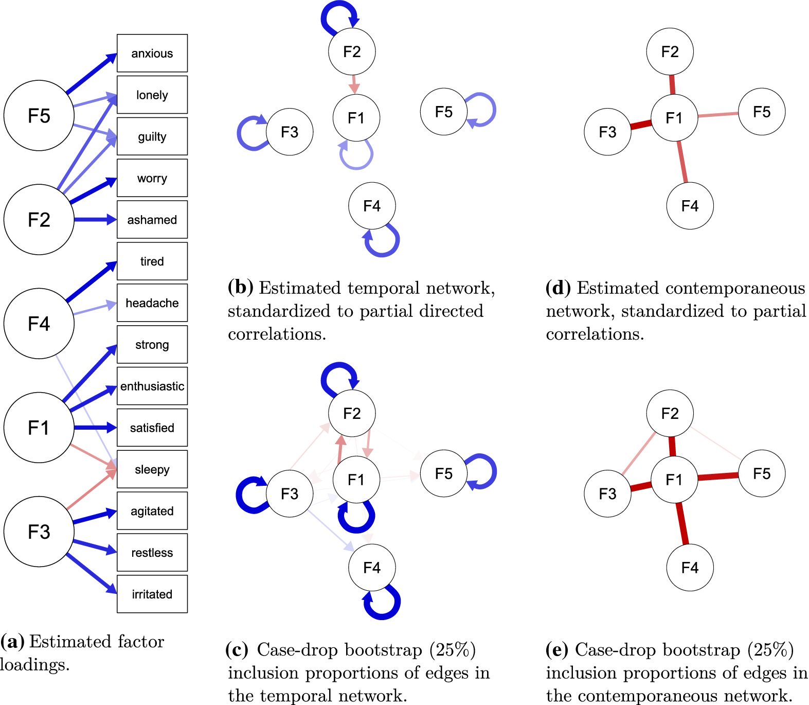
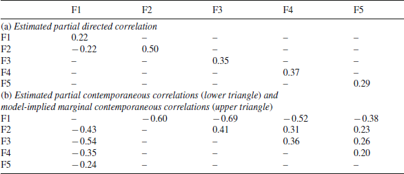
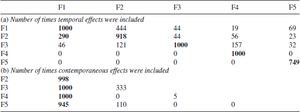
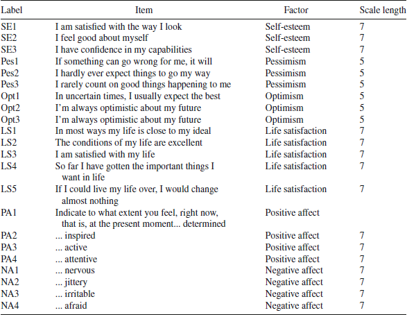
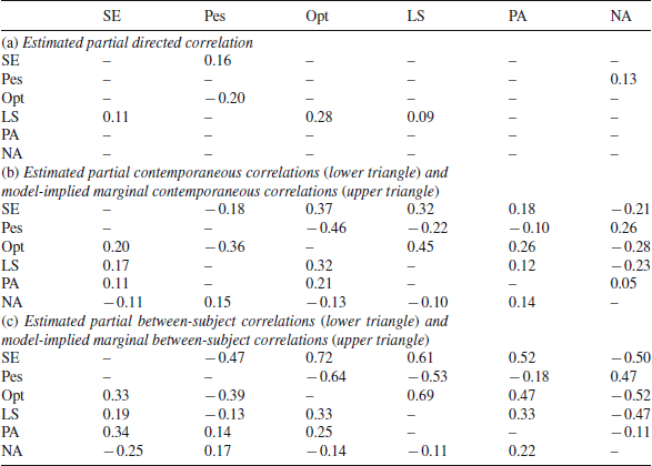

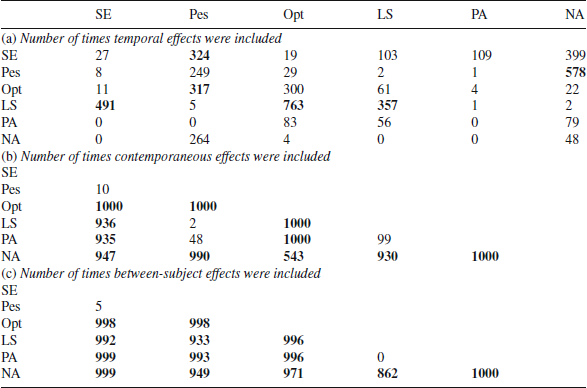


 Open access