

1. Introduction
Adherence to a particular marital-specific subgroup is closely related to exposures affecting mortality patterns, such as healthcare utilization [Iwashyna and Christakis (Reference Iwashyna and Christakis2003); Nihtilä and Martikainen (Reference Nihtilä and Martikainen2008)], labor force participation Van Hedel et al. (Reference Van Hedel, Van Lenthe, Avendano, Bopp, Esnaola, Kovács, Martikainen, Regidor and Mackenbach2015), smoking [Ramsey et al. (Reference Ramsey, Chen-Sankey, Reese-Smith and Choi2018)], and drinking [Dinescu et al. (Reference Dinescu, Turkheimer, Beam, Horn, Duncan and Emery2016)]. This highlights the important policy implications that marital status may have for health system design, social and labor market policies, clinical care, and pension transfer policies. The advantages in survival probabilities enjoyed by married individuals compared to singles have been well documented in the literature. Never married, divorced, and widowed individuals face higher mortality rates than married individuals, see e.g. Hu and Goldman (Reference Hu and Goldman1990), Johnson et al. (Reference Johnson, Backlund, Sorlie and Loveless2000), and Murphy et al. (Reference Murphy, Grundy and Kalogirou2007). These differences are usually more pronounced for men than for women. The lower mortality for married individuals is explained by two main reasons: the effects of selection of low-risk individuals into the marriage state [Goldman (Reference Goldman1993)], and the protective effects of marriage [Espinosa and Evans (Reference Espinosa and Evans2008)].
Although the topic of married versus single has been extensively studied, questions about the effect of cohabitation remain open. Brown and Wright (Reference Brown and Wright2017) provide a literature review on the importance of cohabitation status. A growing proportion of individuals classified as never married, divorced, and widowed are in fact living with a partner. This leads to considerable changes in partnership status and living arrangements [Cherlin (Reference Cherlin2010)]. Therefore, it is increasingly important to understand the effects of these trends on changes in mortality. Wu et al. (Reference Wu, Penning, Pollard and Hart2003) study the selection and protection effects of both cohabitation and marriage. They find that the selection effect only accounts for a small proportion of the variation in health between the marital states whereas the protection effect is found to be the most likely source of health benefits from marriage and cohabitation. In the literature on survival and cohabitation, most studies are based on duration models investigating the death rates, see e.g., Koskinen et al. (Reference Koskinen, Joutsenniemi, Martelin and Martikainen2007), Scafato et al. (Reference Scafato, Galluzzo, Gandin, Ghirini, Baldereschi, Capurso, Maggi and Gino2008), Drefahl (Reference Drefahl2012), and Frisch and Simonsen (Reference Frisch and Simonsen2013). All these studies treat cohabitation as a homogeneous group and neglect to distinguish the living arrangements prior to entering the cohabitation state. Moreover, Booth et al. (Reference Booth, Hyndman, Tickle and De Jong2006) compare the death rates and life expectancies among several variants and extensions of the Lee–Carter method and find that significant differences in death rates do not necessarily translate into significant differences in life expectancies.
One key area where marital status plays an important role is healthcare utilization toward end-of-life. The costs of healthcare expenditures are continuously rising [Martin et al. (Reference Martin, Hartman, Lassman and Catlin2021)]. Combined with increasing life expectancies there is a growing concern over the impact on future sustainability of healthcare systems. According to French et al. (Reference French, McCauley, Aragon, Bakx, Chalkley, Chen, Christensen, Chuang, Côté-Sergent, De Nardi, Fan, Échevin, Geoffard, Gastaldi-Ménager, Gørtz, Ibuka, Jones, Kallestrup-Lamb, Karlsson, Klein, de Lagasnerie, Michaud, O'Donnell, Rice, Skinner, van Doorslaer, Ziebarth and Kelly2017), total healthcare spending accounted for approximately 17% and 11% of GDP in 2011 in the United States and Denmark, respectively. Out of the total lifetime healthcare spending, 17–22% was spent on people in the last three years of life. However, married spouses have the potential to limit the expenditure levels, as they are more likely to serve as informal caregivers [see Wachterman and Sommers (Reference Wachterman and Sommers2006)]. Studies of end-of-life healthcare show that married individuals are less likely to be in nursing homes [Freedman (Reference Freedman1996)], use higher quality hospitals, and have shorter lengths of hospital stay [Iwashyna and Christakis (Reference Iwashyna and Christakis2003)]. In light of the aforementioned wrong classification of singles, this raises the question of whether cohabiting spouses serve as informal caregivers to the same degree as married individuals.
The purpose of this paper is twofold. First, we examine how marital status, particularly cohabitation, affects the expected remaining lifetime (i.e., life expectancy) of individuals. Second, we investigate how long-term care medical expenditures are distributed between marital groups. Using the unique, extensive Danish register data, we are able to identify marriage and cohabitation history of all individuals in the Danish population. Thus, in addition to marriage, we define three single state categories (divorced, widowed, and never married) and three cohabitation state categories (cohabiting-divorced, cohabiting-widowed, and cohabiting-never married). For each of the seven marital groups, we calculate marital-specific life expectancies. To the best of our knowledge, we are the first to consider different types of cohabitation states and to investigate the effect these states have on life expectancy rather than on mortality rates. Ultimately, life expectancies are more informative in terms of understanding the direct consequences of mortality differences. To validate statistical differences, we apply Welch's t-tests which account for differences in the variances across living arrangements. The extensive nature of the Danish register data also provides individual information on long-term care utilization. This allows us to conduct a unique case study on the importance of cohabitation when analyzing end-of-life long-term care medical spending. In particular, we consider the end-of-life healthcare expenditures on home help and retirement homes for all individuals dying in 2012 in the 12 months prior to death and examine how these expenditures vary across living arrangements. The differences in expenditures between marital groups are validated based on statistical testing.
We find that on average, all cohabiting individuals enjoy higher life expectancies compared to their single counterparts, i.e., compared to widowed, divorced, and never married individuals that live alone. This result holds for both genders and across age groups. However, compared to married individuals, the size and significance of differences in life expectancies vary. For both genders, cohabiting-widowed individuals are on average living as long as married individuals whereas the life expectancy of cohabiting-divorced individuals is statistically lower compared to married individuals. For cohabiting-never married individuals, the results are mixed depending on gender and age group. In general, our results indicate that simply categorizing all unmarried individuals as single would overestimate their remaining lifetime as it neglects to account for the increasingly important cohabitation group. Moreover, we find that this group is particularly important when considering end-of-life long-term care expenditures: Our results suggest that cohabiting spouses serve as informal caregivers to the same degree as married spouses. Specifically, we find that regardless of cohabitation type, their average costs on home help and retirement homes are equal to those of the married group. Compared to all types of non-cohabiting singles, long-term care expenditures are much lower for married and cohabiting individuals. Thus, cohabitation does indeed contribute to reducing end-of-life long-term care costs and may hold the potential to improve health outcomes and maximize the efficiency of healthcare provision.
Our results point to a number of relevant applications beyond healthcare utilization. In particular, governments and pension funds rely heavily on accurate forecasts of longevity as they have guaranteed individuals a lifelong income stream independently of how long they live. Failing to account for mortality patterns within different marital groups thus challenge the pension fund's ability to manage their longevity risk effectively and price their pension products. For governments, marital status plays an important role in the multi-pillar pension systems as it aims at reducing financial inequality across subgroups by letting pension payments from pillar one be means tested against household income.
The rest of the paper is organized as follows: section 2 presents the data and methodology. The life expectancies for the different marital and cohabiting groups and the results on the significance tests are given in section 3. The case study on the long-term care costs is provided in section 4, and section 5 concludes.
2. Data and method
We use the extensive register data from Statistics Denmark that tracks each individual in the Danish population through a Central Person Register number. We consider all individuals above age 49 in the time period 1982–2019. The individual-specific data contain information on age, gender, year, time of death, and marital and cohabiting status. We define seven different marital states: married, widowed, divorced, never married, cohabiting-widowed, cohabiting-divorced, cohabiting-never married. Individuals are tracked over time as their marital status changes. This is one of the many advantages of using the Danish register data: it provides detailed information throughout an individual's lifespan, and not just, e.g., at the time of death. Thus, we allow individuals to move between the different states until two years prior to death. This assumption avoids flows toward the single groups in the year of death. The importance of tracking individuals over time and accounting for transitions between marital states rather than focusing on one stage in life (death) is discussed in Robards et al. (Reference Robards, Evandrou, Falkingham and Vlachantoni2012). Brown and Wright (Reference Brown and Wright2017) also highlight that increases in divorce rates at older ages make the static marital status as a proxy for longevity risk less appropriate.
A cohabiting couple is defined using the following definition by Statistics Denmark: (1) they live at the same address, (2) they are of opposite sex, (3) the age difference is less than 15 years, (4) they are not closely related, (5) no other adults (above age 18) live at the address. If two individuals who live together have shared children living at the same address, these individuals are also characterized as a cohabiting couple (regardless of the criteria listed above).
Table 1 shows the yearly average, minimum, and maximum counts of exposures and deaths for the period 1982–2019 for the entire Danish population above age 49 for females and males. Here, exposures refer to the number of people at risk of dying in a particular marital-gender subgroup. Each year, we consider on average 1,245,213 females with 27,120 deaths and 945,323 males with 26,297 deaths. The largest group consists of married individuals for both females and males. The fact that females are on average living longer than males causes the number in the widowed female group to be higher: it is almost as large as the married female group. Moreover, this effect is also driven by the age difference for married couples in which females are typically the youngest.
Yearly average, minimum, and maximum exposure and death counts for the period 1982–2019 for the total Danish population above age 49

In order to visualize demographic changes over time, Figure 1 plots the percentage share of married, cohabiting, and single individuals of the entire Danish population above age 49. Since the percentage share of cohabiting individuals is very low compared to married and single individuals, we have plotted the married (blue) and single (green) series on the left axis, while the cohabiting series (red) is plotted on the right axis. The figure shows that there is a small but consistent movement from the married to the cohabitation state (especially after 2008), while the single group is relatively stable over time (percentage share around 35%).
Percentage share of married, cohabiting, and single individuals in the total Danish population above age 49. Source: Statistics Denmark–StatBank.dk/FAM100N.

We group all individuals into 5-year age intervals to avoid few deaths at older ages and top-coded the data at age 95. Thus, we define the age intervals $a_{x}\in \left\{50\hbox {-}54,\; 55\hbox {-}59,\; \ldots ,\; 95 + \right\}$ where x refers to a specific age at the lower bound of an age interval. For each age interval, a x, and year, t ∈ {1982, 1983, … , 2019}, we calculate marital-specific death rates:

for i = {married, widowed, divorced, never married, cohabiting-widowed, cohabiting-divorced, cohabiting-never married}. The number of deaths in group i is denoted by d i(t, a x) and E i(t, a x) denotes the exposure for group i. Note that, when disaggregating individuals into seven marital groups for each gender, the cohabitation classifications display very few deaths for some years. Consequently, the corresponding death rates and life expectancies become noisy. In the Internet Appendix IA.2, we show life expectancies based on death rates that are smoothed over the year dimension using P-splines [Eilers and Marx (Reference Eilers and Marx1996)].Footnote 1
The purpose of this paper is to investigate the effect of marital status on the remaining lifetime (i.e., life expectancy) of an individual at a given age, x. Thus, we calculate period life expectancies for each of the seven marital groups using standard life table techniques [see Preston et al. (Reference Preston, Heuveline and Guillot2001)]. The period life expectancy at age x is a recursive function, f, of the age interval death rates in (1) at all age intervals above age x:

Note that here h = 5 is the width (in years) of the age intervals and $\bar {x} = 95$ is the lower bound of the last age interval. We assume that deaths occur half way through the age interval. For more details, we refer to Preston et al. (Reference Preston, Heuveline and Guillot2001), pages 38–51. Life expectancy calculations are based on artificial cohorts, since we compute period life expectancies (i.e., using all age-specific death rates in a given year). Thus, if an individual changes marital group from one year to the next, he/she will contribute to the life expectancy calculation of two different martial groups in two different years. In this paper, we calculate period life expectancies at ages 50 and 70.Footnote 2
Note that we calculate period life expectancies as opposed to cohort life expectancies. As discussed in Pitacco et al. (Reference Pitacco, Denuit, Haberman and Olivieri2009), period life expectancies are based on a set of age-specific death rates for a given year, and therefore do not allow for future changes in mortality. On the contrary, cohort life expectancies allow for changes in mortality in later years, since these are based on a set of age-specific death rates of a given cohort. However, this advantage comes at the cost of estimation and projection errors: in order to get cohort life expectancies in later periods, one needs to rely on projections of future death rates for a given cohort [see Pitacco et al. (Reference Pitacco, Denuit, Haberman and Olivieri2009), for details]. Using mortality data for the US and Sweden, Goldstein and Wachter (Reference Goldstein and Wachter2006) show that cohort life expectancies are consistently higher compared to period life expectancies. Using Danish data, Alvarez et al. (Reference Alvarez, Kallestrup-Lamb and Kjærgaard2021) look at the indexation of the retirement age based on life expectancies. They confirm the result that cohort life expectancies are higher compared to period life expectancies, but argue that the size of the gap between the two methods is not overwhelming.
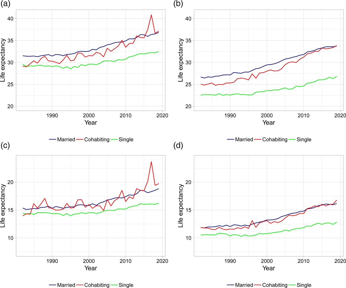
Figure 2 plots gender-specific life expectancies at ages 50 and 70 for married, singles, and cohabitors. The figure confirms results previously found in the literature: married and cohabiting individuals live longer lives compared to singles with a gap in life expectancies of 2.5–7.5 years in 2019. This difference is more pronounced for men than women: the difference in gap size between men and women is up to 3 years in 2019. In this paper, we elaborate on these findings by investigating how different types of living arrangements affect the life expectancy patterns, and whether these effects are statistically significant.
Life expectancies at age 50 and 70 for married, singles, and cohabitors. (a) Female LE at age 50. (b) Male LE at age 50. (c) Female LE at age 70. (d) Male LE at age 70. Note: Life expectancies are based on 5-year age interval death rates.
2.1 Welch's t-test
We use Welch's t-test [Welch (Reference Welch1947)] to formally test whether the differences in life expectancy among various living arrangements are significant. In general, Welch's t-test tests whether two groups have equal means while allowing for unequal sample sizes and variances. Alternatively, we could have performed a classical ANOVA test [Fisher (Reference Fisher1925)] of equality in means between groups. However, ANOVA assumes that the sample sizes and variances in all groups are equal. The constant variance assumption is unlikely to be fulfilled in our case, since we expect the variances of life expectancies to differ across the different living arrangements. In particular, we will see in the figures below that the cohabitation groups have higher standard deviations. A similar argument holds for the sample size.
Booth et al. (Reference Booth, Hyndman, Tickle and De Jong2006) perform single and multiple t-tests (ANOVA) to determine whether several distinct methods for forecasting life expectancies are equal to the actual, realized life expectancies. They show that a direct translation of significant differences in mortality rates to significant differences in expected lifetime do not exist. This substantiates our choice of testing for significant differences in life expectancies.
The test statistic between the life expectancies of group i and j is defined as

where $\bar {e}^{i}( x)$ is the life expectancy sample mean over years and $s^2_{\bar {e}^{i}( x) }$
 is the sample standard error. The latter is defined by the sample standard deviation, $s_{e^{i}( x) }$
 , divided by the square root of the sample size, N i: $s_{\bar {e}^{i}( x) } = s_{e^{i}( x) }/\sqrt {N_i}$
 . Here N i = 2019 − 1982 + 1 = 38 for all groups i. We perform two-tailed tests for all combinations of married and cohabiting groups (as first term i) versus all single groups (as second term j)Footnote 3 for different ages using actual death rates for life expectancy calculations.
3. Results
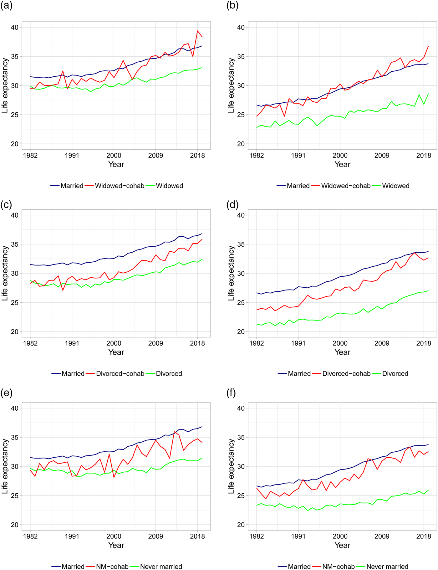
As the first in the literature, we present life expectancy calculations for different types of cohabiting individuals. Figures 3 and 4 show the period life expectancies at ages 50 and 70, based on 5-year age interval death rates as described in section 2. The left panels show female life expectancies and the right panels show male life expectancies. Panels (a) and (b) plot life expectancies for married, widowed, and cohabiting-widowed individuals, panels (c) and (d) plot life expectancies for married, divorced, and cohabiting-divorced individuals, and panels (e) and (f) plot life expectancies for married, never married, and cohabiting-never married individuals. In Table 2, we calculate the average life expectancy at age 50 over the first 5 years (i.e., 1982–1986) and the last 5 years (i.e., 2015–2019) along with the associated improvement rates.
Life expectancies at age 50 based on actual death rates. (a) Female LE for married, widowed, and cohabiting-widowed. (b) Male LE for married, widowed, and cohabiting-widowed. (c) Female LE for married, divorced, and cohabiting-divorced. (d) Male LE for married, divorced, and cohabiting-divorced. (e) Female LE for married, never married, and cohabiting-never married. (f) Male LE for married, never married, and cohabiting-never married. Note: Life expectancies are based on 5-year age interval death rates.
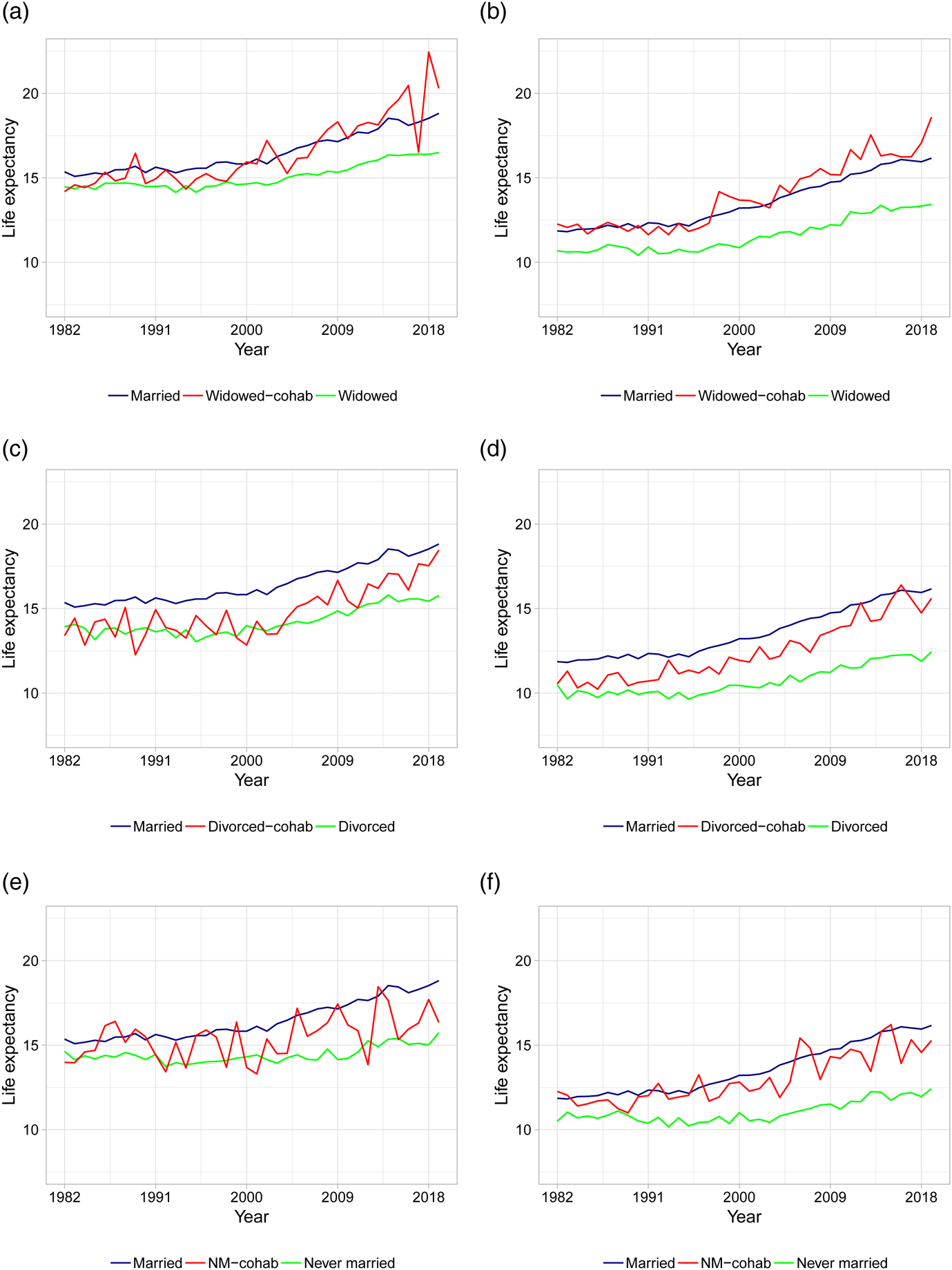
Life expectancies at age 70 based on actual death rates. (a) Female LE for married, widowed, and cohabiting-widowed. (b) Male LE for married, widowed, and cohabiting-widowed. (c) Female LE for married, divorced, and cohabiting-divorced. (d) Male LE for married, divorced, and cohabiting-divorced. (e) Female LE for married, never married, and cohabiting-never married. (f) Male LE for married, never married, and cohabiting-never married. Note: Life expectancies are based on 5-year age interval death rates.
Average LE at age 50 for the first and last 5 years and corresponding improvement rates

Note: Life expectancies are based on actual 5-year age interval death rates. The improvement rates are calculated as the percentage increase between the 1982–1986 average and the 2015–2019 average.
Before discussing the results, recall that there are two channels that can explain the life expectancy differences between married or cohabitors and singles: the protection effect and the selection effect. Wu et al. (Reference Wu, Penning, Pollard and Hart2003) study how much each of these channels attribute to the health variations between married or cohabiting individuals and single individuals. They find that the selection effect only accounts for a small proportion of the variation, whereas the protection effect is found to be the most likely source of health benefits of marriage and cohabitation. Throughout this paper, we will refer to the protection effect when discussing life expectancy variations between married or cohabitors and singles, keeping in mind that it also encompasses the selection effect.
We first consider age 50 in Figure 3 and Table 2. From Figure 3 it is clear that marriage is associated with the highest life expectancies compared to non-married individuals, with the exception of cohabiting-widowed individuals who follow more or less the same pattern as married individuals. In the beginning of the period, the remaining life expectancy for married individuals is around 31 years for females and 27 years for males compared to below 30 for single females and below 24 for single males. This confirms the general finding in the literature that marriage offers protection compared to being single [see, e.g., Hu and Goldman (Reference Hu and Goldman1990)].
Focusing on cohabitors, we observe that in the beginning of the period, cohabitation offers little or no protection for females: the life expectancies for all types of cohabiting females are close to that of the non-cohabiting singles (see Figure 3). In particular, the gaps in life expectancy between each type of female cohabitors and singles are at most 1/3 of a year (whereas the gaps between married and singles are more than 1.5 year, see Table 2). This suggests that there is no protective effect of cohabitation for females in the beginning of the period. For males, the gaps in life expectancy between each type of cohabitors and singles are all larger than 2 years, suggesting that cohabitation offers protection for males in the beginning of the period. The largest gaps in male life expectancies is found for cohabiting-widowers and cohabiting-never married compared to their single counterparts.
Toward the end of the period, the life expectancies in Figure 3 for all types of cohabitors (both genders) seem to be either equal to or close to that of the married. Considering Table 2, we observe that the gaps in life expectancy between each type of female cohabitors and singles have increased to more than 2.5 years. Thus, in later years we see that cohabitation does indeed offer protection for females. Married females are still living the longest with a gap to singles of 3.5–5.5 years. The largest gaps are between married or cohabiting-widowed and widowed females. For males, the protective effect of cohabitation and marriage has increased substantially over the time period. In particular, the gaps in life expectancy between married or cohabitors and singles are all above 6 years. For married or cohabiting-widowed males, the gaps to widowed males are as high as 7.5–8 years.
In general, life expectancies are increasing over time for all groups. However, as evident from Table 2, there are large differences in the life expectancy improvement rates across gender and living arrangements. The improvement rates are generally higher for males compared to females. For both genders, cohabiting-widowed and cohabiting-divorced individuals have experienced the most rapid increases in life expectancies with improvement rates above 0.25 for females and 0.35 for males. In comparison, the improvement rates for married individuals are 0.16 for females and 0.26 for males. The improvement rates for cohabiting-never married individuals are similar to those of the married. The smallest improvements are found for the widowed and especially the never married individuals with rates as low as 0.06 for females and 0.09 for males.
As a robustness check, Figure 4 shows the life expectancies at age 70. As evident from the figure, the patterns are similar compared to the younger age group, although the variability is higher due to less individuals in older age groups.Footnote 4
In conclusion, males appear to always benefit from living with someone. Over time, the number of extra years enjoyed by married and cohabiting males has increased. For females, the protective effect of cohabitation only emerges in later years. However, for both genders the sizes of life expectancy differences and the rapidness of the increases in life expectancies vary depending on cohabitation type. Thus, these findings accentuate that failing to recognize the heterogeneity that exists within the non-married group is problematic which opposes against labeling cohabitors as singles. In order to investigate statistical significances, we perform Welch's t-tests, since it can be difficult to distinguish whether or not differences in life expectancies are significantly meaningful.
3.1 Test results
In Tables 3 and 4 we display test results based on Welch's t-test for ages 50 and 70, respectively. For each combination of living arrangement, we test the null hypothesis of “no difference between life expectancies” versus there being a difference. The tests are based on the life expectancies as shown in Figures 3 and 4. The tables include the test statistics and the corresponding p-values in parentheses for a two-tailed test. Those cells that are depicted in gray present non-significant differences at a significance level of 5% and black cells indicate a significant difference in life expectancies.
Welch's t-test of no difference between life expectancies at age 50 for female (upper panel) and male (lower panel)

Note: Life expectancies are based on actual 5-year age interval death rates.
Welch's t-test of no difference between life expectancy at age 70 for female (upper panel) and male (lower panel)

Note: Life expectancies are based on actual 5-year age interval death rates.
Based on the tests, we can conclude that for the entire period altogether, cohabitation is proven to be protective compared to being single (we reject the null, see diagonal elements in Tables 3 and 4). Moreover, married individuals are in most cases living statistically significantly longer than those who are cohabiting (see first column in both tables). However, for widowed individuals living with a spouse is equally as protective as being married (we cannot reject the null). This also holds for never married males at age 70.
As we saw in the plots of the life expectancies, the figures become more noisy as the groups age because of fewer individuals. All figures and tests displayed so far are based on the actual death rates over 5-year age intervals. In the Internet Appendix IA.1 and IA.2 we show the test results and the associated life expectancies based on death rates that are smoothed over the year dimension. For marital groups which contain a large number of individuals, the smoothing algorithm confirms our conclusions based on the actual death rates. However, when there are fewer individuals in a specific group, such as never married females, the smoothing algorithm fails to produce robust results.
The p-values of the Welch's t-test displayed in the tables represent the values for the two-sided hypothesis test. When we want to draw conclusions on relative differences between life expectancies, we need to convert the alternative hypothesis. The test statistics remain unchanged for the one-sided alternative while the p-values should be adjusted depending on the desired sign of the inequality of the alternative hypothesis and the sign of the t-statistic. Recall that the test is constructed as the life expectancy of those who are married minus one of the other living arrangements, either cohabiting or single. When those who are cohabiting are compared to singles, the test is constructed as the cohabitors minus the singles. Hence, a significant and positive t-statistic implies a rejection against the alternative hypothesis that the difference in life expectancies is positive. The associated one-sided p-value is, in that case, simply the one displayed in the tables divided by two. A significant and negative t-statistic would imply that the null hypothesis is rejected against the life expectancy difference being negative. Here, all significant tests are positive which indicates that a statistical difference between, e.g., cohabitation and singles implies that cohabitors live longer than singles and not the other way round.
4. Case study: long-term care
Most developed countries are experiencing population aging [United Nations (2019)], as life expectancy is increasing. The risk of dying during post-retirement ages has trended downwards [Rau et al. (Reference Rau, Soroko, Jasilionis and Vaupel2008); Zuo et al. (Reference Zuo, Jiang, Guo, Feldman and Tuljapurkar2018)], such that individuals from more recent cohorts spend a longer time in retirement compared to previous ones [Sanderson and Scherbov (Reference Sanderson and Scherbov2010, Reference Sanderson and Scherbov2017)]. In Denmark, like most other European countries, the old-age dependency ratioFootnote 5 is currently at around 30% and forecasted to increase further to 50% in 2070.Footnote 6 In line with this development, the costs of national healthcare expenditures are continuously rising [Martin et al. (Reference Martin, Hartman, Lassman and Catlin2021)]. In 2011, 11% of Danish GDP was spent on the healthcare system while 22% of the total healthcare expenditures was spent on people in the last 3 years of life [see French et al. (Reference French, McCauley, Aragon, Bakx, Chalkley, Chen, Christensen, Chuang, Côté-Sergent, De Nardi, Fan, Échevin, Geoffard, Gastaldi-Ménager, Gørtz, Ibuka, Jones, Kallestrup-Lamb, Karlsson, Klein, de Lagasnerie, Michaud, O'Donnell, Rice, Skinner, van Doorslaer, Ziebarth and Kelly2017)]. Thus, there is a growing concern over the impact on future sustainability of healthcare systems.
Although the population aged 65 and above consume healthcare resources at a much higher rate, these older individuals also hold a potential to limit the expenditure levels as married spouses are more likely to serve as informal caregivers [see Wachterman and Sommers (Reference Wachterman and Sommers2006)]. However, an increasing number of individuals are misclassified as singles even though they are in fact living with a spouse, see Figure 1. Scarce information about unmarried cohabiting couples has prevented researchers from investigating the support function of cohabitation. Moreover, given the protective effect of both marriage and cohabitation in terms of life expectancy shown above, there are reasons to suspect that healthcare utilization and thus healthcare expenditures too will differ by marital status. As the first in the literature, we show how end-of-life long-term care (LTC) expenditures vary across different types of singles including cohabitation. In particular, we estimate the mean annual LTC spending that occurs in the final year of life. These costs typically increase substantially close to death as the majority of older people experience declining health and progressive disability at the end of their lives, see Lunney et al. (Reference Lunney, Lynn, Foley, Lipson and Guralnik2003).
Note that sharing of resources among spouses (like health insurance benefits or finances) is not a concern in our study as the Danish healthcare system is characterized as a Beveridgian model. Thus, taxes finance healthcare costs, and citizenship enables free and equal access to universal health insuranceFootnote 7. Moreover, this limits the effect of bequest motives on the distribution of LTC utilization and expenditures between marital groups. In other countries, such as the US, bequests play a significant role in the demand for long-term care [see Groneck (Reference Groneck2017)].
This study uses unique register data on long-term care supplied by Statistics Denmark for the years 2011 and 2012. The registers contain individual-level information for the entire Danish population allowing us to link anonymized data at the individual level on demographics such as age, gender, and marital status to information on various forms of long-term care. On home care and home nurses, we have access to number of hours supplied on a daily basis from the municipality. These services are delivered either in people's own homes or in residential housing for the elderly. We group these two categories into one, labeled home help. Moreover, we have access to a register that identifies whether individuals were residents in nursing homes or residential homes for the elderly during the year. We label this category retirement homes.
The registers do not contain specific information on expenditures. Instead we assess total expenditures on LTC by combining information from OECD Health Data (categories HC3.1 and HC3.2) with expenditure information from the Danish Ministry of Health (2009, 2010) and the Danish Economic Council (2009) as in French et al. (Reference French, McCauley, Aragon, Bakx, Chalkley, Chen, Christensen, Chuang, Côté-Sergent, De Nardi, Fan, Échevin, Geoffard, Gastaldi-Ménager, Gørtz, Ibuka, Jones, Kallestrup-Lamb, Karlsson, Klein, de Lagasnerie, Michaud, O'Donnell, Rice, Skinner, van Doorslaer, Ziebarth and Kelly2017). Thus, we allocated these imputed costs to individuals based on the micro data on nursing home incidence, and hours of use of home care and home nurses, respectively.Footnote 8 All numbers are inflated to 2014 price levels. We consider our imputation of LTC at the individual level to be the best possible given the information available. To determine health expenditures as individuals approach the time of death, we acknowledge that medical spending in a given year of death does not represent a full year of expenses.Footnote 9 Therefore, we exploit the daily nature of the register data to track the 2012 death cohort over their last 12 months prior to death (covering the years 2011 and 2012) and calculate their LTC costs. We observe 47,794 decedents above the age of 49 in 2012.
During the last couple of decades, it has been a deliberate policy of the Danish government to keep elderly individuals in their own homes for as long as possible [Rostgaard et al. (Reference Rostgaard, Glendinning, Gori, Kröger, Osterle, Szebehely, Thoebald, Timonen and Vabo2011)] and when necessary provide support from home careers, home nurses, etc. Nursing homes are more costly and reserved for the very fragile and ill elderly [Nielsen et al. (Reference Nielsen, Bekker-Jeppesen, Almer and Andreasen2016)]. Therefore, only a small fraction of a cohort will be residents in such a home. Figure 5 shows the average cost spent on home help or retirement homes out of all individuals who passed away in 2012. Thus, within each marital group, the total costs on home help and retirement homes are both divided by the total number of individuals dying in that group. By conditioning on those who died we are able to infer which martial group had the highest level of consumption of a given expenditure type. Note that the figure does not display the average cost of e.g. placing an individual in a retirement home. This would be uninformative for our comparison as the average costs conditional on residing in a retirement home are unlikely to differ significantly between marital states.
Average 1-year medical spendings on home help and retirement homes per individual for all individuals dying in 2012. Note: Numbers are reported in US Dollars and 2014 price levels. The average age in each group is from left to right for females 73, 76, 68, 64, 86, 75, 77 and for males 76, 79, 70, 64, 84, 70, 69.

The average 1-year medical spendings on LTC per individual for the 2012 death cohort are displayed in Figure 5. We find that cohabiting individuals have lower LTC cost in the last 12 months of their lives compared to non-cohabiting singles. The gray bar represents expenditures to home help and the blue bar to retirement homes. Thus, singles that are cohabiting display a spending pattern that closely mimic the behavior of married individuals. Never married individuals that are cohabiting show the lowest spendings across all types of marital groups whereas widowed individuals display the highest level of spendings. Among the married and cohabiting individuals, cohabiting-widows stand out as the home help expenditures are much higher compared to married and cohabiting-divorcees and never married. This indicates that cohabiting-widows do not to the same extent receive informal care from their cohabiting male spouses.
Singles spend on average two and a half times as much on long-term care compared to married and cohabiting individuals. In particular, we find that singles on average spend almost twice as much on home help and four times as much on retirement homes. It is clear from Figure 5 that women to a larger degree serve as informal caregivers as married and cohabiting males have lower average costs. Finally, we see that single women have higher average LTC costs compared to men reflecting the higher life expectancies of females. We apply the Welch's t-test to determine whether expenditures are in fact significantly different. We confirm that this indeed is the case and the results can be found in Appendix A, Tables A.1, A.2, and A.3.
The demand and need for care will increase dramatically over the next decades as a result of changing population demographics [European Commission (2020)]. This will likely change the availability of informal caregivers in the future. Understanding variations in long-term care expenditures between and within different types of singles are important when evaluating the economics of end-of-life care. Our results strongly suggest that not only married individuals but also singles that are cohabiting have the potential to limit the expenditure levels due to the level of informal care they provide.
5. Conclusion
An increasing number of couples living together are unmarried. While married couples are relatively easy to identify due to the legal aspects of marriage, cohabiting couples are more difficult to track down. However, since cohabitation is increasing in popularity and is expected to share some of the same health benefits as marriage, it is essential to understand and account for cohabitors when analyzing, e.g., mortality patterns, labor force participation, and healthcare utilization.
In this paper, we use the unique, extensive Danish register data to analyze the effect of various living arrangements on life expectancy and end-of-life long-term care expenditures. In particular, we identify married, cohabiting, and single individuals and subdivide the cohabitors and singles into widowed, divorced, and never married leading to seven different marital states. For each state, we calculate marital-specific life expectancies and test for statistical differences in life expectancies between the groups. Next, we utilize the detailed nature of the Danish registers in order to conduct a case study on how long-term care expenditures on home help and retirement homes during the last 12 months of life are distributed by marital groups.
Our findings suggest that cohabiting individuals benefit in terms of life expectancy from living with a spouse compared to being single. Living arrangements prior to entering the cohabitation state determines the size and significance of the differences in life expectancies between cohabiting and married individuals. In particular, we find that on average cohabiting-widowed individuals live as long as married individuals, whereas cohabiting-divorced individuals have significantly lower life expectancies compared to married individuals. Additionally, we find that the improvement rates in life expectancy are largest for cohabitors. The case study on long-term care expenditures toward end-of-life also emphasizes the importance of accounting for cohabitation, as the results show that cohabiting individuals have much lower costs compared to singles, while costs are similar between cohabitors and married. These results hold for all cohabitation types. Thus, the function of informal caregivers within the household is not restricted to married individuals, but also plays a significant role for all types of cohabiting individuals.
The understanding of life expectancy trends and patterns is essential for making accurate longevity forecasts. For both the pension industry and governments, these forecasts are crucial in terms of managing their longevity risk. Our paper contributes by highlighting the importance of recognizing life expectancy variations across different types of marital groups and particularly cohabitation. Related to healthcare budgeting, our case study on long-term care expenditures toward the end-of-life shows that there are large differences in expenditures between married or cohabitors and singles. This information is beneficial for both clinicians in terms of evaluating individual needs for care and for public health professionals when assessing and predicting future healthcare expenditures.
In conclusion, our findings represent a significant step toward understanding how marital status and in particular cohabitation affects life expectancy and long-term care expenditures, and the paper facilitates further research in various aspects. In terms of classifying marital groups, future studies could consider same sex couples, remarried couples, couples with children, and socioeconomic status combined with marital status. There are several methodological challenges related to these classifications, which include small sample sizes and the need for strong assumptions when determining who belongs to which group. In our case study, we investigated one important cost component of society: long-term care. There are various alternative issues that could be investigated. These include how hospital and pharmaceutical expenditures are distributed according to marital groups, the smoking and drinking behavior within each group, and an analysis on causes of death by marital group.
Supplementary material
The supplementary material for this article can be found at https://doi.org/10.1017/dem.2023.10
Acknowledgements
We are grateful to the anonymous referee for the valuable comments and suggestions. We also thank participants at the 16th International Longevity Risk and Capital Markets Solutions Conference, 2021, Copenhagen (Denmark); the 8th International Conference on Mathematical and Statistical Methods For Actuarial Science and Finance, 2018, Madrid (Spain); and the 13th International Longevity Risk and Capital Markets Solutions Conference, 2017, Taipei (Taiwan) for their feedback and comments.
Appendix
A.1. Case study: testing
Welch's t-test of no difference between medical spendings on home help

Welch's t-test of no difference between medical spendings on retirement homes

Welch's t-test of no difference between aggregate medical spendings on home help and retirement homes


 Open access