


1. Introduction and motivation
Numerical and experimental form-finding methods for structures made of membranes, cables, trusses and/or sheets have been a widely adopted part of architectural design and engineering for many decades.
Form finding may be defined as “a forward process in which parameters are explicitly/directly controlled to find an ‘optimal’ geometry of a structure which is in static equilibrium with a design loading.” (Reference Adriaenssens, Block, Veenendaal and WilliamsAdriaenssens et al., 2014). Typically, real world loads (dead load and typical live load) are used as design loading.
To optimally make use of sheets’ or membranes’ load-bearing capacity, typically uniform stress distributions are prescribed (thereby also excluding bending stresses) during this form-finding (optimization) process. Similarly, in a lightweight engineering context like in automotive or aerospace engineering, utilization of material strength is a target. However, commonly used plastics and alloys in this fields are much more robust when subjected to bending loads as opposed by architectural materials like concrete and cables. In addition, slenderness ratios tend to be lower.
For this work, we want to focus on components predominantly consisting of thin-walled closed surfaces. For many such components, wall thickness will be dictated by the manufacturing process (like casting or injection moulding) rather than loading. So, material will be mechanically underutilized regardless of the design (at least in most areas). Under such conditions, choosing a minimal surface wherever possible will be an efficient approach for lightweight design. However, the necessity to fulfil the minimal surface condition everywhere (for strength reasons) can be relaxed.
Even if stresses are the limiting factor, using a minimal surface wherever possible as an initial design might be an effective starting point. Optimizing wall thickness and/or shape according to strength requirements might then be a second optimization step (which is outside of the scope of this work).
One qualification used above deserves additional elaboration: We argued that using minimal surfaces wherever possible was a beneficial choice. In this work, one requirement frequently impeding the use of actual minimal surfaces will be considered: Typical thin-walled components like housings or covers are naturally shaped by the components they are intended to enclose or cover. In addition, only rarely can components be designed completely freely, that is without consideration of design space restrictions. This is particularly natural for the industries under consideration in this work. Among the numerous extensive works published on form finding like (Reference BletzingerK.-U. Bletzinger, 2024), (Reference VeenendaalVeenendaal, 2017), (Reference RippmannRippmann, 2016) and (Reference Adriaenssens, Block, Veenendaal and WilliamsAdriaenssens et al., 2014), (Reference Bletzinger and RammK. U. Bletzinger & Ramm, 2001), none were identified directly respecting such constraints. Instead, use of space was controlled indirectly by constraints and the topology (makeup of shells/sheets and trusses/cables) of the design. We, in contrast, will respect design space restrictions directly in the proposed iterative form-finding implementation. To the best of the authors’ knowledge, this integration has not been published before. These restrictions will be implemented as contact constraints between the surface under optimization and a representation of the non-design space (see Section 2). The utility of this will be further discussed in Section 3.
In addition, shell-like components might frequently incorporate “linear”, i.e. sweeping-like features. For example, a cover component might require a flange for mounting. The cross-sectional area of the flange profile might be given by technological and functional requirements (like bolt and/or sealing dimensions). The masses contributed by such linear structure can be represented similar to cables in form-finding processes. The implementation proposed in this work will demonstrate this, too. While this interpretation as purely weight-minimization instrument is novel, the inclusion of such elements per se is not novel in the context of form-finding. In fact, cable models are among the oldest form finding models (Reference Veenendaal and BlockVeenendaal & Block, 2012), (Reference RippmannRippmann, 2016).
2. Implementation based on standard FEA software
From the above elaborations one might already expect a FEA model would be able to solve the problem. Indeed, the iterative use of such a model was already described in (Reference Tabarrok and QinTabarrok & Qin, 1992). he use of basic FEA software intended for structural analysis in form finding has also been described in (Reference Levy and SpillersLevy & Spillers, 1998). Essentially, the proposed method is an implementation of a stiffness matrix method as described in (Reference VeenendaalVeenendaal, 2017) and (Reference Adriaenssens, Block, Veenendaal and WilliamsAdriaenssens et al., 2014). A force density method covered in the same works and further elaborated for example in (Reference Wüchner and BletzingerWüchner & Bletzinger, 2005) was not applied in this work. This choice was made to demonstrate ease of implementation. Basic FEA solvers should be accessible to most engineers in most organizations involving some amount of mechanical engineering.
2.1. Theoretical justification
In the following, it shall be shown that the problem is actually solved by repeatedly carrying out a specific FEA calculation: Let us consider a set of two-dimensional elastic entities of constant thickness like shells or membranes
 $${{\rm{S}}^{3{\rm{D}}}}$$
and a set of one-dimensional elastic entities of constant cross-section like beams and rods
$${{\rm{S}}^{3{\rm{D}}}}$$
and a set of one-dimensional elastic entities of constant cross-section like beams and rods
 $${{\rm{S}}^{2{\rm{D}}}}$$
sufficiently constrained in three-dimensional space by boundary conditions. We then change the state by subjecting the entities (without displacement) to elastic pre-strains: 2-dimensional entities get pre-strained biaxially by
$${{\rm{S}}^{2{\rm{D}}}}$$
sufficiently constrained in three-dimensional space by boundary conditions. We then change the state by subjecting the entities (without displacement) to elastic pre-strains: 2-dimensional entities get pre-strained biaxially by
 $${\rm{\varepsilon }}_{{\rm{xx}}}^{2{\rm{D}}} = {\rm{\varepsilon }}_{{\rm{yy}}}^{2{\rm{D}}} = {{\rm{\varepsilon }}^{2{\rm{D}}}}$$
, one-dimensional entities by longitudinal strains
$${\rm{\varepsilon }}_{{\rm{xx}}}^{2{\rm{D}}} = {\rm{\varepsilon }}_{{\rm{yy}}}^{2{\rm{D}}} = {{\rm{\varepsilon }}^{2{\rm{D}}}}$$
, one-dimensional entities by longitudinal strains
 $${\rm{\varepsilon }}_{{\rm{xx}}}^{1{\rm{D}}} = {{\rm{\varepsilon }}^{1{\rm{D}}}}$$
. Putting in Hooke’s Law and assuming plane stress, this new state exhibits the stresses (Equation 1)
$${\rm{\varepsilon }}_{{\rm{xx}}}^{1{\rm{D}}} = {{\rm{\varepsilon }}^{1{\rm{D}}}}$$
. Putting in Hooke’s Law and assuming plane stress, this new state exhibits the stresses (Equation 1)

Then, a static equilibrium is obtained by solving for a suitable displacement field
 $${\rm{u}}\left( {\rm{x}} \right)$$
. Note that this equilibrium state, per definition, will be have minimal total Energy
$${\rm{u}}\left( {\rm{x}} \right)$$
. Note that this equilibrium state, per definition, will be have minimal total Energy
 $${\rm{W}}\left( {\rm{u}} \right)$$
given the imposed constraints, boundary conditions and material laws. This new spacial configuration (exhibiting non-homogenous stresses and strains) is now kept fixed while re-applying the homogenous strain and stress state given above. Iterating this process will typically converge. Without further theoretical investigation, the possibility of divergence (oscillations or chaotic behaviour) cannot be excluded categorically. However, no indications of such behaviours were observed during any experiments.
$${\rm{W}}\left( {\rm{u}} \right)$$
given the imposed constraints, boundary conditions and material laws. This new spacial configuration (exhibiting non-homogenous stresses and strains) is now kept fixed while re-applying the homogenous strain and stress state given above. Iterating this process will typically converge. Without further theoretical investigation, the possibility of divergence (oscillations or chaotic behaviour) cannot be excluded categorically. However, no indications of such behaviours were observed during any experiments.
One notable special case can and will occur however within the realm of convergence in the sense described here: The geometry might approach a state of topological change. Parts of the surface might collapse into lines (or points). This, however, is more of a practical than a fundamental problem as these areas will not contribute to the energies this section is operating on.
When the process has converged, that is,
 $${\rm{u}} \approx 0$$
, it follows that the pre-stressed state already satisfies the equilibrium condition while still minimizing total energy. This energy exclusively exists in the form elastic potential of the form
$${\rm{u}} \approx 0$$
, it follows that the pre-stressed state already satisfies the equilibrium condition while still minimizing total energy. This energy exclusively exists in the form elastic potential of the form
 $${\rm{W}} = \frac{{1}\over{2}}\sum {{\rm{c}}_{{\rm{ij}}}}{{\rm{\varepsilon }}_{\rm{i}}}{{\rm{\varepsilon }}_{\rm{j}}}{\rm{V}}$$
. Concretely, the total energy can be given as (Equation 2)
$${\rm{W}} = \frac{{1}\over{2}}\sum {{\rm{c}}_{{\rm{ij}}}}{{\rm{\varepsilon }}_{\rm{i}}}{{\rm{\varepsilon }}_{\rm{j}}}{\rm{V}}$$
. Concretely, the total energy can be given as (Equation 2)

From this, it is obvious that if we had chosen material properties and strain loading appropriately, that is, so that (Equation 3)
 $${\rm{\sigma }}_{\rm{i}}^{2{\rm{D}}}{\rm{\varepsilon }}_{\rm{i}}^{2{\rm{D}}} = \frac{{1}\over {2}}{\rm{\sigma }}_{\rm{j}}^{1{\rm{D}}}{\rm{\varepsilon }}_{\rm{j}}^{1{\rm{D}}},\forall {\rm{i}},{\rm{j}}$$
by virtue of minimizing total energy, we have obtained a configuration of minimum total volume. All entities of each category may share the same parameters, so for simplicity the according indices
 $$i,j$$
are dropped from now on. The following choices were made for this work (Equation 4):
$$i,j$$
are dropped from now on. The following choices were made for this work (Equation 4):

The decision for a common stress value
 $${\rm{\sigma }}$$
was primarily motivated by the comfort of visualizing stresses to estimate convergence in a postprocessor.
$${\rm{\sigma }}$$
was primarily motivated by the comfort of visualizing stresses to estimate convergence in a postprocessor.
2.2. Implementation
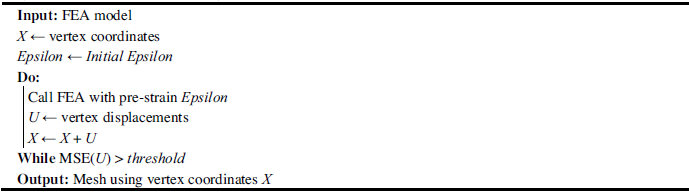
The process was automated using Python. The essential procedure can be written as:
iterative form-finding:

The FEA model essentially contains a meshed initial design. One load case is defined where the prescribed Epsilon
 $$= {{\rm{\varepsilon }}^{1{\rm{D}}}} = 2{{\rm{\varepsilon }}^{2{\rm{D}}}}$$
is applied by means of a temperature field.
$$= {{\rm{\varepsilon }}^{1{\rm{D}}}} = 2{{\rm{\varepsilon }}^{2{\rm{D}}}}$$
is applied by means of a temperature field.
2.3. Application on problems with known analytical solutions: catenoids
Catenoids are minimal surface with a known analytical representation. They therefore present themselves as prime candidates for testing the proposed method.
2.3.1. Basic analytical problem
Any surface fulfilling the condition (Equation 5)

connects any pair of contained circles (which are their intersections with planes parallel to the xy-plane) locally minimally, i.e. any variation of the surface conserving its topology will increase its area. Given a pair of circles there may be two solutions for
 $$c$$
and
$$c$$
and
 $${\rm{\zeta }}$$
. The one with the larger absolute value of
$${\rm{\zeta }}$$
. The one with the larger absolute value of
 $$c$$
is stable and can be obtained physically by simple and well-known soap film experiments. This solution can also be expected to be found numerically.
$$c$$
is stable and can be obtained physically by simple and well-known soap film experiments. This solution can also be expected to be found numerically.
All following calculations and investigations will be presented without units. The suitable power of the length unit will be easily derived from context. As the problem is of rotational symmetry and we will not break this symmetry, the following will only be presented in cylindrical coordinates. The two circles (Equation 6)
 $$\left( \matrix{{{{r_1}}} \cr {{{\rm{z}}_1}}} \right) = \left( \matrix{{120} \cr { - 50}} \right),\left( \matrix{{{r_2}} \cr {{{\rm{z}}_2}}}\right) = \left( {\matrix{{80} \cr {50}}} \right)$$
were chosen as boundaries. The above catenoidal equation is not easily solved for
 $$c$$
and
$$c$$
and
 $$\zeta $$
analytically. Hence, Maxima, an open-source computer algebra system, was used. A Newton-Raphson algorithm was employed to obtain the solutions for
$$\zeta $$
analytically. Hence, Maxima, an open-source computer algebra system, was used. A Newton-Raphson algorithm was employed to obtain the solutions for
 $${c_{\rm{i}}}$$
and
$${c_{\rm{i}}}$$
and
 $${\zeta _i}$$
. The resulting functions of all examples of this chapter are shown in the left plot of Figure 1 in the form
$${\zeta _i}$$
. The resulting functions of all examples of this chapter are shown in the left plot of Figure 1 in the form
 $$r = {f_i}\left( z \right)$$
. The two functions
$$r = {f_i}\left( z \right)$$
. The two functions
 $${f_1}$$
and
$${f_1}$$
and
 $${f_2}$$
show the stable and unstable solution of the described problem without added constraints.
$${f_2}$$
show the stable and unstable solution of the described problem without added constraints.
2.3.2. Design space restriction
To simulate design space limitations, a torus given by (Equation 7)
 $${\left( {{\rm{r}} - 60} \right)^2} + {{\rm{z}}^2} = {35^2} = {\rm{r}}_{{\rm{minor}}}^2$$
was considered as non-design space. Note that from the minimal surface condition it follows that the solution must be
 $${c_1}$$
-continuous (given the
$${c_1}$$
-continuous (given the
 $${c_1}$$
-continuity of the torus itself). The parameters of the solution
$${c_1}$$
-continuity of the torus itself). The parameters of the solution
 $${f_3}$$
, which can be represented piecewise analytically were obtained numerically. The crosses in the plot of Figure 1 indicate points where the solution is in fact only
$${f_3}$$
, which can be represented piecewise analytically were obtained numerically. The crosses in the plot of Figure 1 indicate points where the solution is in fact only
 $${c_1}$$
-continuous, that is, where the analytical solutions are stitched. A dotted indication of the torus is also shown in the plot.
$${c_1}$$
-continuous, that is, where the analytical solutions are stitched. A dotted indication of the torus is also shown in the plot.
2.3.3. “Linear” features contributing to weight
As described in Section 1, linear features should be included in the optimization. This was implemented by adding a ring with a cross-sectional area of 20 to the model. Based on the considerations of Section 2.1, the equilibrium was again calculated numerically, resulting in
 $${f_4}$$
in Figure 1. Note that this result is only
$${f_4}$$
in Figure 1. Note that this result is only
 $${c_0}$$
-continuous at the intersection of the branches. The branches must be symmetrical as a direct consequence of the force equilibrium at this intersection point. The symmetry plane is given by
$${c_0}$$
-continuous at the intersection of the branches. The branches must be symmetrical as a direct consequence of the force equilibrium at this intersection point. The symmetry plane is given by
 $${\rm{z}} \approx 19.545$$
where the function reaches its minimum value
$${\rm{z}} \approx 19.545$$
where the function reaches its minimum value
 $${\rm{r}} \approx 68.277$$
.
$${\rm{r}} \approx 68.277$$
.
Catenoidal shapes, analytical solutions (left) and optimization results (right)

Figure 1 Long description
Panel A: The line graph displays multiple curves representing different functions. The horizontal axis is labeled z with a range from -50 to 50. The vertical axis is labeled r with a range from 0 to 120. The graph includes five different curves labeled f0, f1, f2, f3, and f4, each with distinct colors and styles. The curves show various trends and intersections within the plotted range. Panel B: The 3D shapes include four distinct geometries. The top left shape is brown, the top right shape is purple, the bottom left shape is green, and the bottom right shape is blue. Each shape has a unique, complex form with visible surface details.
2.3.4. Numerical solution in 3D space
The process described in Section 2.2 was executed. For the independent parameters discussed there, (Equation 8)

were chosen. As a initial configuration, a conical mesh fulfilling the boundary conditions as shown in Figure 1 as
 $${f_0}$$
was used. It consists of
$${f_0}$$
was used. It consists of
 $$26\times 157 = 4082$$
quadrilateral membrane elements of edge length
$$26\times 157 = 4082$$
quadrilateral membrane elements of edge length
 $$l = 4$$
and is depicted in the right part of the figure in the top left. Initially, bilinear quadrilateral elements (S4) were used. Based on this, the solutions of the three posed problems (
$$l = 4$$
and is depicted in the right part of the figure in the top left. Initially, bilinear quadrilateral elements (S4) were used. Based on this, the solutions of the three posed problems (
 $${f_1}$$
,
$${f_1}$$
,
 $${f_3}$$
,
$${f_4}$$
$${f_3}$$
,
$${f_4}$$
 ) could be approximated with varying accuracy. Final meshes are depicted in Figure 1 in the right matching the order and color of the plots on the left side.
Overview over some errors (mean squared, after 128 iterations)

Table 1 shows an overview over the errors based on this procedure. The following sections will detail experiments and conclusions.
2.3.5. Choice of Poisson number
Different choices of Poisson Numbers
 $${\rm{\nu }}$$
were investigated. As can be seen in Figure 2, choosing a larger value without exception resulted in faster convergence. This is to be expected as the mesh will have to stretch in the axial direction while contracting in the radial direction. Also, larger Poisson Numbers tended to yield smaller final errors. The figures show a root mean squared error. As underlying measurement only the radial deviation of the mesh vertices from the precise solution was considered. Averaging was then performed over all mesh points of the model.
$${\rm{\nu }}$$
were investigated. As can be seen in Figure 2, choosing a larger value without exception resulted in faster convergence. This is to be expected as the mesh will have to stretch in the axial direction while contracting in the radial direction. Also, larger Poisson Numbers tended to yield smaller final errors. The figures show a root mean squared error. As underlying measurement only the radial deviation of the mesh vertices from the precise solution was considered. Averaging was then performed over all mesh points of the model.
Errors over iterations for
 $${f_1}$$
(left) and
$${f_1}$$
(left) and
 $${f_4}$$
(right)
$${f_4}$$
(right)

2.3.6. Element type considerations
Based on the above investigations, the use of various element types was evaluated, resulting in the following conclusions: In comparison to shell elements (S4), membrane elements (M3D4) showed indistinguishable behavior of the optimization process. However, some optimizations (not shown) struggled to converge using membranes. Concretely, deliberately unfavourably chosen (“wavy”) initial configurations promoted wrinkling behavior, which could not be suitably represented. Generally, it was deemed advisable to use shells instead of membranes to avoid stability problems which are clearly more prevalent in the absence of bending stiffness. The shell thickness was chosen as 1 in the models used in this section, so bending stiffness was still reasonably small. Scaling shell thickness might serve as a convenient way to improve convergence should issues occur in practice. Decreasing thickness again and ultimately switching to membranes at a later stage of the optimization should be beneficial, but no recognizable benefit could be devised from such experiments.
Distinct refinement strategies were investigated: The left plot in Figure 2 shows the convergence behavior of different models for the single catenoid problem
 $${f_1}$$
. Here, P1 denotes the basis models with an edge length of
$${f_1}$$
. Here, P1 denotes the basis models with an edge length of
 $$l = 4$$
and linear shell elements (S4). P2 denotes models of the same resolution using second order elements (S8R). Finally, P1h denotes the use of a h-refined first order mesh. Here,
$$l = 4$$
and linear shell elements (S4). P2 denotes models of the same resolution using second order elements (S8R). Finally, P1h denotes the use of a h-refined first order mesh. Here,
 $$l = 2$$
was chosen, resulting in a quadrupled number of elements. Based on these results, clearly, the model benefits from a p-refinement strategy much more than from h-refinement. This contrasts the premise that “owing to the greater geometric nonlinearity of membrane structures, it is preferable to use a dense mesh of primitive elements rather than a coarse mesh made up of higher order elements” given in (Reference Tabarrok and QinTabarrok & Qin, 1992). However, given the total model dimension in the range of
$$l = 2$$
was chosen, resulting in a quadrupled number of elements. Based on these results, clearly, the model benefits from a p-refinement strategy much more than from h-refinement. This contrasts the premise that “owing to the greater geometric nonlinearity of membrane structures, it is preferable to use a dense mesh of primitive elements rather than a coarse mesh made up of higher order elements” given in (Reference Tabarrok and QinTabarrok & Qin, 1992). However, given the total model dimension in the range of
 $${10^2}$$
, all three models could likely suffice in an engineering setting of the problem of
$${10^2}$$
, all three models could likely suffice in an engineering setting of the problem of
 $${f_1}$$
.
$${f_1}$$
.
Turning to the convergence behaviour of problem
 $${f_4}$$
with added rod/truss elements (T3D2) displayed in right plot of Figure 2 may give a substantially different interpretation. Here, the errors of the initial model do not drop below
$${f_4}$$
with added rod/truss elements (T3D2) displayed in right plot of Figure 2 may give a substantially different interpretation. Here, the errors of the initial model do not drop below
 $$ \sim 1.7$$
. Interestingly, h-refinement does not yield any improvement. In fact, errors even increased by
$$ \sim 1.7$$
. Interestingly, h-refinement does not yield any improvement. In fact, errors even increased by
 $$ \sim 5\% $$
. Both models significantly overestimate the radial necking caused by the ring of trusses. The smallest diameter was underestimated by
$$ \sim 5\% $$
. Both models significantly overestimate the radial necking caused by the ring of trusses. The smallest diameter was underestimated by
 $$ \sim 3.8\% $$
, already hinting at a underestimation of the forces present in the doubly curved shell section. The axial position of the smallest diameter deviated 1.21 from the true solution.
$$ \sim 3.8\% $$
, already hinting at a underestimation of the forces present in the doubly curved shell section. The axial position of the smallest diameter deviated 1.21 from the true solution.
In contrast, the use of second order elements brought errors down to a level which should be acceptable in most applications. Here, using a larger Poisson Number not only accelerated convergence but also yielded in noticeably smaller errors. The smallest diameter was estimated with an error of
 $$only\;0.02\% $$
, its position deviated only
$$only\;0.02\% $$
, its position deviated only
 $$0.078$$
from the true axial position.
$$0.078$$
from the true axial position.
Generally, the error values obtained based on the radial deviation of the result from the theoretical result should be interpreted with care when only the optimization target (minimal volume) is of concern. Concretely, the final error of P1 with
 $${\rm{\nu }} \approx 0.5$$
was
$${\rm{\nu }} \approx 0.5$$
was
 $$1.75$$
(linear length units) after 128 iterations. However, this seemingly excessive deviation only amounted to an added volume of 26.5, which represents
$$1.75$$
(linear length units) after 128 iterations. However, this seemingly excessive deviation only amounted to an added volume of 26.5, which represents
 $$0.036\% $$
of the total volume. When comparing the results to the initial cone configuration, this is equivalent to leaving only
$$0.036\% $$
of the total volume. When comparing the results to the initial cone configuration, this is equivalent to leaving only
 $$0.49\% $$
of the total optimization potential unexploited. Note that the volume here is composed of the shell area scaled by its thickness and the truss length scaled with the given cross-sectional area.
$$0.49\% $$
of the total optimization potential unexploited. Note that the volume here is composed of the shell area scaled by its thickness and the truss length scaled with the given cross-sectional area.
2.3.7. Contact (i.e. non-design space) model
Aside from pragmatic advantages, the implementation based on structural FEA enables the straightforward implementation of non-design regions as rigid bodies in contact with the mesh under optimization. This was shown successfully by the optimization of
 $${f_3}$$
. A frictionless linear contact model with stiffness of
$${f_3}$$
. A frictionless linear contact model with stiffness of
 $${10^4}$$
(pressure per length unit) was used. A rigid (bi-)linear quadrilateral shell mesh was used as contact partner representing the torus given in Section 2.3.2 and Abaqus’ surface-to-surface contact formulation was used. Considering the previous choices
$${10^4}$$
(pressure per length unit) was used. A rigid (bi-)linear quadrilateral shell mesh was used as contact partner representing the torus given in Section 2.3.2 and Abaqus’ surface-to-surface contact formulation was used. Considering the previous choices
 $${\rm{\sigma }} = 100$$
and
$${\rm{\sigma }} = 100$$
and
 $${r_{{\rm{minor}}}} = 35$$
the above stiffness should give a contact penetration of
$${r_{{\rm{minor}}}} = 35$$
the above stiffness should give a contact penetration of
 $$ \sim 3 \cdot {10^{ - 4}}$$
, which was well reproduced by the model. From further experiments the following conclusions were made:
$$ \sim 3 \cdot {10^{ - 4}}$$
, which was well reproduced by the model. From further experiments the following conclusions were made:
Convergence of the models with contacts was much faster when compared to the previous models. All models of
 $${f_3}$$
could be deemed converged after just 16 iterations. This can be understood as the contact effectively splits the problem into smaller sub-problems.
$${f_3}$$
could be deemed converged after just 16 iterations. This can be understood as the contact effectively splits the problem into smaller sub-problems.
Surface-based contact modeling was superior to a node-based model, which showed approximately twice the error. This can be explained with the reduced penetration in surface-based contact, thereby mitigating the error caused by geometric discretization.
Significant benefit was also derived from refining the contact mesh. The errors given in Table 1 were obtained with a contact mesh of
 $$l = 4$$
, matching the resolution of the optimization mesh. Halving the edge length reduced the error by almost one order of magnitude to
$$l = 4$$
, matching the resolution of the optimization mesh. Halving the edge length reduced the error by almost one order of magnitude to
 $$ \sim 5 \cdot {10^{ - 3}}$$
. This can be at least partially explained by the reduction of the maximum surface deviation of the contact mesh from
$$ \sim 5 \cdot {10^{ - 3}}$$
. This can be at least partially explained by the reduction of the maximum surface deviation of the contact mesh from
 $$0.057$$
for
$$0.057$$
for
 $$l = 4$$
to
$$l = 4$$
to
 $$0.014$$
for
$$0.014$$
for
 $$l = 2$$
. As a conclusion, using a finer contact mesh (than optimization mesh) is advisable.
$$l = 2$$
. As a conclusion, using a finer contact mesh (than optimization mesh) is advisable.
2.8.3. On the interpretation of forces
Even if forces occurring in the models do not carry inherent mechanical meaning, they still can be interpreted meaningfully: A single force of value
 $$F$$
acting in the converged model is equivalent to a truss of cross-sectional area
$$F$$
acting in the converged model is equivalent to a truss of cross-sectional area
 $$A = \sigma /F$$
pulling in the same direction. From this, forces can be interpreted as follows:
$$A = \sigma /F$$
pulling in the same direction. From this, forces can be interpreted as follows:
 $$F/\sigma $$
gives the sensitivity of the minimized part volume with respect to a translation (in the direction of
$$F/\sigma $$
gives the sensitivity of the minimized part volume with respect to a translation (in the direction of
 $$F$$
) of the constraint (which is causing the reaction force
$$F$$
) of the constraint (which is causing the reaction force
 $$F$$
).
$$F$$
).
Concretely, the total axial reaction force at the boundaries in the
 $${f_1}$$
problem using the second order Model (P2) is
$${f_1}$$
problem using the second order Model (P2) is
 $${F_y} \approx 48281.1$$
, resulting in a sensitivity of
$${F_y} \approx 48281.1$$
, resulting in a sensitivity of
 $${\rm{d}}V/{\rm{d}}{z_2} = {F_y}/{\rm{\sigma }} \approx 482.811$$
. The analytical model gives the same solution (again numerically obtained) up to an impressive relative error of the order
$${\rm{d}}V/{\rm{d}}{z_2} = {F_y}/{\rm{\sigma }} \approx 482.811$$
. The analytical model gives the same solution (again numerically obtained) up to an impressive relative error of the order
 $${10^{ - 6}}$$
. In contrast to this, both of the first order models (P1 and P1h) underestimate the reaction force by
$${10^{ - 6}}$$
. In contrast to this, both of the first order models (P1 and P1h) underestimate the reaction force by
 $$ \sim 15.0\% $$
. No reduction in error was observed due to mesh refinement. This is consistent with the increased necking observed in the problem of
$$ \sim 15.0\% $$
. No reduction in error was observed due to mesh refinement. This is consistent with the increased necking observed in the problem of
 $${f_4}$$
. Linear elements seem to consistently underestimate the forces generated by the doubly curved shell under biaxial prestress. This result underscores the necessity to use second order models to represent phenomena that include Neumann-type boundaries.
$${f_4}$$
. Linear elements seem to consistently underestimate the forces generated by the doubly curved shell under biaxial prestress. This result underscores the necessity to use second order models to represent phenomena that include Neumann-type boundaries.
3. Towards solving realistic engineering problems: differential gear housing
To demonstrate the utility of the proposed process, a somewhat realistic engineering problem was posed and solved:
3.1. Problem definition
Given the core functional components of a differential gear, a design of a housing is to be developed. The components are shown in the left image of Figure 3, the bounding box of this model is approximately
 $$200 \times 182 \times 143$$
. Displayed in orange color are regions representing bearings which support the shafts visualized in turquoise. These bearings should themselves be supported by the housing under design. The rest of the design sketch represents the gears and differential assembly. It is assumed that the large gear and differential assembly (shown in blue) should be assembled in a straight motion from the back (right) before closing the housing using a cover. The cover will connect to the housing at a flange of given cross-section 216. Note that this value was later recognized to be geometrically unfeasibly large but kept for consistency. The wall thickness of the housing and cover should be 3. The housing and cover should keep a minimum clearance of 5 mm from the inner components as well as their paths during assembly.
$$200 \times 182 \times 143$$
. Displayed in orange color are regions representing bearings which support the shafts visualized in turquoise. These bearings should themselves be supported by the housing under design. The rest of the design sketch represents the gears and differential assembly. It is assumed that the large gear and differential assembly (shown in blue) should be assembled in a straight motion from the back (right) before closing the housing using a cover. The cover will connect to the housing at a flange of given cross-section 216. Note that this value was later recognized to be geometrically unfeasibly large but kept for consistency. The wall thickness of the housing and cover should be 3. The housing and cover should keep a minimum clearance of 5 mm from the inner components as well as their paths during assembly.
Core components (left) and derived non-design spaces (right)

3.2. Design space considerations
To represent this clearance requirement, two separate bodies were used. These are shown in the right image of Figure 3. Both bodies are based on simple offsets from the components. The lavender body represents the non-design space relevant for the housing. This includes the hull of the large gear and cage assembly for assembly as well as the small gear. The green body will be used as non-design space for the cover. Note that the shafts were (inconsistently but irrelevantly) only part of the latter body.
3.3. The initial design
For this demonstration, a hand crafted initial design for the optimization was created using Autodesk Fusion. This initial design is shown in Figure 4 on the left. It already fulfills all design space constraints described above. Note that this was done with minimal effort: Excluding fillets, it only consists of a total of five basic elements (extrusions and revolutions). Also, it connects to the inner edges of the bearing geometries, which will serve as boundary conditions for the optimization.
The surface bodies shown in Figure 3 were then meshed using Abaqus CAE. The collision bodies (Figure 3 right) were represented using quadrilateral meshes (not shown) using R3D4 elements. The subject of optimization (Figure 4 left) was meshed using a triangular mesh. This initial mesh is shown in Figure 5 on the left. A total of 82 637 elements were used. For this demonstration, in discrepancy with the learnings of Section 2.3.6, first order finite elements (S3) were used. To represent the flange in the model, truss elements (T3D2) were added to the line separating the housing region mesh from the cover region mesh. These truss elements were not well visualized in the used post processing software (Abaqus CAE), so they are not displayed in the figures. Their location is indicated by the pronounced kink in the meshes due to their influence and the change in constraints at the same location.
CAD surface models: initial design (left) and reconstructed optimization result (right)

3.4. Optimization runs
Two optimization runs performed, each was run for 256 iterations taking between three and four hours of computing time on a mid-range laptop computer. In the first run, the flange’s position was fixed. So, all vertices at the separation line had only active degrees of freedom in their common plane. In the second run, one degree of freedom was added, i.e. the position of this common plane. In both runs the flange was kept planar and constrained parallel to its original position.
Both results are displayed in Figure 5 next to the initial mesh. Colored in red are the areas where the mesh is in contact with non-design space mesh. Everywhere else (except for the edge representing the flange), the mesh represents a local minimal surface with mean curvature of
 $$ \approx 0$$
.
$$ \approx 0$$
.
Optimization meshes: initial design (left), result with fixed flange position (center), result with free flange position (right)

Table 2 shows the improvements in total volume (including the flange). The second optimization moved the flange plane towards the output shafts for a further reduction in mass, illustrating the power of the method of giving designers non-trivial, global input for improvement of designs. The flange position is given relative to the axis of the output shafts.
Optimization results

3.5. Reconstruction and CAD design
To demonstrate an actual design, a solid CAD model was created. The first optimization result described above was split into housing and cover parts. These were then extrapolated at the boundaries. The meshes were then converted to spline faces using Autodesk Fusion (Figure 4 right). A flange guide curve was extracted from the faces. Then flanges and hull bodies were created before appropriately joining the bodies. After some minor cleanup, the housing geometry shown in Figure 6 was obtained.
3D CAD reconstruction of an optimization result

Figure 6 Long description
A cross-sectional view of a 3D CAD reconstruction showing an optimization result. The outer layer is yellow with a textured surface. Inside, there are multiple components in different colors: blue, green, and light blue. The blue component is centrally located and surrounded by other components. The green component is positioned above the blue one, and the light blue components are distributed around the central blue component. The arrangement suggests a complex internal structure with non-homogenous stresses and strains.
4. Summary and discussion
This work proposes a workflow for form-finding in a mechanical design engineering setting focussed on saving weight. It extends known form-finding methods by including non-design space utilizing a contact model. Readily available tools were utilized for the entire procedure. In particular, a programming language (Python), a CAD system (Autodesk Fusion) and an FEA solver (Abaqus FEA) were used. Results were validated using examples with known analytical solutions. The process was also demonstrated on a close to real world design problem.
4.1. Learnings and potential applications
The proposed method gives sufficiently precise results to be applied to engineering problems. It was shown that design space constraints can be meaningfully included in a form-finding optimization process. Whenever linear structures or force-like boundaries are included or forces are intended to be interpreted meaningfully second order elements should be used.
The proposed process can serve as a design tool in lightweight engineering of mostly shell-like structures. This might include components like casings, covers and housings as well as handling, moving or packaging equipment of various kinds. It may be of particular interest in cases where mechanical properties of the component are not expected to critically determine the design given the relevant manufacturing constraints (like minimum wall thickness). The process only uses customary engineering software tools facilitating potential adoption.
4.2. Limitations and future work
In this work, manufacturing constraints have not been implemented. This might be of major concern in some contexts, further work will be necessary to appropriately employ manufacturing constraints. Some of these could be represented by adding further design space restrictions. Adding suitable couplings, constraints, or elements to the FEA model without impacting the process as a whole could also represent some of such additional constraints. As a counter-example, demolding constraints are trivial to formulate with respect to geometry (e.g. as a forbidden space for normal vectors), but there is no obvious mechanical analogy for implementing them in a structural analysis as presented. Expanding on this in detail is left for future work.
In addition, the process as shown relies on creating a CAD model from a mesh model. This is an active area of research and may limit the adoption of the method in some contexts. The resulting mesh geometry could also just serve as a guide for the designer.
Requiring hours of compute time instead of seconds, the proposed solution demands high computational cost compared to dedicated form finding algorithms. This may be acceptable in an engineering environment where consistency with a basic (CAD and FEA) set of tools offers a relevant incentive for adoption of form-finding altogether. This inefficiency could be mitigated by applying gradient descent algorithms as is for example done in (Reference Pastrana and AdriaenssensPastrana & Adriaenssens, 2024). This could also further increase flexibility with respect to constraints. However, obtaining gradients is typically not feasible when using a commercial FEA system. For such a solution, a specific FEA solver or an entirely different underlying form-finding procedure would have to be used. Such solutions shall be presented in future works.
The initial design was hand crafted and fairly close to the optimum solution. An efficient implementation of form-finding could generate an initial design with even less effort from constraints only. Recent developments from the field of machine learning show great promise in this area (Reference Berzins, Radler, Volkmann, Sanokowski, Hochreiter and BrandstetterBerzins et al., 2024). An investigation of how these methods could be integrated is also left for future work.
Also left to a further investigation is the question whether partly zero mean curvature shell structures show a clear tendency to benefit or hinder typical desirable mechanical properties like high stiffness, strength and/or eigenfrequencies.



 f1
f1 f4
f4





 Open access

