


1. Introduction
Glaciers are key features of mountain regions around the world, providing an essential water source for downstream environmental and human ecosystems (Immerzeel and others, Reference Immerzeel2020). The ongoing global glacier mass loss (Hugonnet and others, Reference Hugonnet2021) is projected to continue throughout the 21st century and beyond (Hock and others, Reference Hock2019), having direct impacts on water resources, cryosphere-related hazards (Ding and others, Reference Ding2021), downstream ecology (Huss and Hock, Reference Huss and Hock2018) and global sea level rise (WCRP Global Sea Level Budget Group, 2018).
Direct measurements of glacier mass balance provide a critical constraint to modeled projections of 21st century glacier change (e.g. Huss and Hock, Reference Huss and Hock2015); yet these in situ observations are time consuming and logistically intensive (e.g. Huss and others, Reference Huss, Bauder and Funk2009; O'Neel and others, Reference O'Neel2019). Of the more than 200 000 glaciers worldwide, only 241 have been monitored in situ since 2010 (World Glacier Monitoring Service, WGMS), and the majority of those records are based on relatively sparse point observations.
The growing availability of remotely sensed geodetic products offers a promising approach for measuring glacier mass balance over increasingly shorter time intervals and finer spatial scales. Glacier volume change measured using repeat digital elevation models (DEMs) can be interpreted as a glacier-wide mass change over sufficiently long time periods (>10 years) using a constant density conversion (Huss, Reference Huss2013). However, vertical ice flow (the emergence velocity) and firn compaction confound the conversion of surface elevation change to mass change–preventing spatially resolved mass-balance estimates from geodetic methods or glacier-wide balances over short time periods (Cuffey and Paterson, Reference Cuffey and Paterson2010; Sold and others, Reference Sold2013). Previous studies have addressed these limitations by using sparse in situ point measurements of emergence velocities (Beedle and others, Reference Beedle, Menounos and Wheate2014; Réveillet and others, Reference Réveillet2021), relating emergence velocities to mass balance and thinning rates (Sold and others, Reference Sold2013; Pope and others, Reference Pope2016; Belart and others, Reference Belart2017; Sass and others, Reference Sass, Loso, Geck, Thoms and McGrath2017), careful density assumptions (Pelto and others, Reference Pelto, Menounos and Marshall2019) or calculating emergence velocities from ice thickness and surface velocities (Pelto and Menounos, Reference Pelto and Menounos2021).
Many regional-scale glacier evolution models use mass-balance profiles for calibration and testing (Radic and others, Reference Radić2014; Clarke and others, Reference Clarke, Jarosch, Anslow, Radić and Menounos2015; Rounce and others, Reference Rounce, Hock and Shean2020). However, reanalysis efforts of long-term glaciological mass-balance series tend to find that glaciological observations are biased relative to geodetic assessments (Zemp and others, Reference Zemp2013; Klug and others, Reference Klug2018; O'Neel and others, Reference O'Neel2019). Enhancing our understanding of the spatial distributions of mass balance can provide insights into the optimal design and applications of in situ mass-balance programs.
In this study we produced spatially distributed seasonal and annual surface mass-balance estimates of Wolverine Glacier through a mass conservation approach with multiple constraints on firn compaction rates and emergence velocities. The detailed spatial patterns of accumulation and ablation that are revealed highlight how stake-derived mass balances are unable to accurately capture the true patterns of mass balance in topographically complex terrain, providing evidence for an underestimation of ablation in glaciological mass balances.
2. Study area
Wolverine Glacier (15.6 km2) is located within the Kenai Mountains along the coast of south-central Alaska, ~100 km south of Anchorage. The climate is maritime, with average annual temperatures of 1°C and winter accumulation of 2.3 m w.e. (Baker and others, Reference Baker, Peitzsch, Sass, Miller and Whorton2019). The glacier is generally south-facing and has an elevation range of 500–1600 m (Fig. 1). The long-term (2001–20 mean) equilibrium line altitude (ELA) is 1226 m, and the annual ELA has trended toward higher elevations over this time period at a rate of ~60 m decade−1 (McNeil and others, Reference McNeil2016: updated 2022). The average annual point mass balances range from −7.0 m w.e. a−1 near the terminus to +4.3 m w.e. a−1 near the head of the glacier over this time period. The glacier has experienced a cumulative mass loss of −23.2 m w.e. from 1966 to 2020, with −16.3 m w.e. in the 2001–20 period (McNeil and others, Reference McNeil2016).
Wolverine Glacier study area, with inset map showing the location of the Kenai Peninsula, Alaska. Blue dots show locations of mass-balance stakes, with inset letters (A-T, AU, EC) indicating the stake name. The glacier retreated past the lowest long-term site (stake A) in 2010, ending its record. Elevation contours are in meters. Background hillshade is derived from the August 2015 DEM (Table 1). Locations and approximate extents of the upper and lower icefalls are shown.

Intervals over which distributed mass balances were measured, with dates of corresponding DEMs, GPR and USGS mass-balance measurements. All dates are listed in mm/dd/yyyy format. 2016 summer does not have DEM dates listed because it was calculated as the difference between the 2016 winter and 2016 annual balances (see Section 4.3). Changes in mass balance between survey dates (i.e. DEM dates and glaciological balance dates) were accounted for using the mass-balance model described in Section 3.5 and O'Neel and others (Reference O'Neel2019).

3. Data
3.1. Digital elevation models
A total of 12 DEMs were utilized in this study (Table S1; McNeil and others, Reference McNeil2019). Seven DEMs were collected between 2015 and 2020, using airborne LiDAR, structure from motion photogrammetry and high-resolution stereo satellite imagery to resolve annual and seasonal elevation changes (Table 1). These DEMs were coregistered to the 2019 fall DEM using stable, snow-free areas (Nuth and Kääb, Reference Nuth and Kääb2011). This approach allows for a linear shift in x, y and z directions, but does not allow for correction of non-linear offsets (rotation and scaling). We inspected the residual elevation differences in DEM pairs and found no evidence of non-linear artifacts. Coregistration of spring DEMs was difficult due to near complete snow cover over the surveyed areas (e.g. Pelto and others, Reference Pelto, Menounos and Marshall2019). Thus, for spring DEMs, three to four coincident stable features were identified (e.g. boulders, the research hut), and a constant x/y/z offset based on the average from those points was used to manually align the spring DEMs to the fall 2019 DEM. Five additional fall DEMs between 1972 and 2012 were used for calculation of long-term elevation changes (Section 4.2) and were coregistered relative to each other prior to differencing using the approach of Nuth and Kääb (Reference Nuth and Kääb2011). A static glacier outline, corresponding to the fall 2019 glacier extent, was used for all analyses.
3.2. End-of-winter snow depths
End-of-winter snow depths were measured using ground-penetrating radar (GPR) in the spring of three years (Table 1) as described in McGrath and others (Reference McGrath2018). Common-offset GPR surveys were conducted using 500 MHz antennas from a snowmobile or helicopter. Survey tracks were similar each year, with an attempt to collect data spanning the full range of glacier terrain parameters (elevation, aspect, slope, etc.) while minimizing objective hazards (crevasses, avalanches).
The radargrams were processed using ReflexW-2D (Sandmeier Geophysical Research) to apply time-zero corrections, dewow and manually pick the boundary between seasonal snow and firn/ice to extract two-way travel time (twt). Snow pits, shallow snow cores and probe observations provided layer-picking validation within radargrams. Column-averaged snow densities were measured in ~5 snow pits and cores across the glacier surface each year. Snow densities exhibited minimal variation and lacked a consistent spatial or elevation dependency, thus a single density from the average of all pits and cores was used for the entire glacier each year (McGrath and others, Reference McGrath2018) for calculating twt and converting snow depth to m w.e. (Helfricht and others, Reference Helfricht, Kuhn, Keuschnig and Heilig2014).
Snow depth, SD, was calculated as:

from the twt and the radar velocity (v s). v s was calculated from an empirical relationship based on the measured densities (Kovacs and others, Reference Kovacs, Gow and Morey1995) and direct comparison between observed in situ snow depth and twt at probe and core locations (McGrath and others, Reference McGrath2018).
Snow depth observations were extrapolated across the glacier surface using a terrain-based statistical extrapolation where terrain parameters are used as proxies for the physical processes that distribute snow across the landscape (Erickson and others, Reference Erickson, Williams and Winstral2005; McGrath and others, Reference McGrath2015). Terrain parameters (elevation, curvature, northness, eastness and wind scouring and drifting potential) were calculated from a fall 2015 DEM downsampled to 10 m resolution using a median filter, and the same values were used each year. GPR snow depth observations in each year were similarly aggregated by taking the median of all observations within each 10 m pixel. GPR-derived snow depths, normalized for elevation dependencies, were then extrapolated across the glacier surface each spring using a regression tree that utilized terrain parameters as independent variables (e.g. Balk and Elder, Reference Balk and Elder2000). For further details on the extrapolation methods, refer to McGrath and others (Reference McGrath2018).
3.3. Mass-balance stakes
Mass-balance stakes were used to measure seasonal and annual point balances from 1966 to present. These point balance measurements were used to derive mass-balance profiles and glacier-wide mass-balance solutions (O'Neel and others, Reference O'Neel2019). For the majority of the record measurements occurred at three sites, but in ~2010 the network was expanded to a total of seven stake sites, with additional stakes added in some years (Fig. 1).
In addition to mass-balance measurements, stake locations were surveyed seasonally over the 1975–96 and 2015–21 periods. Point values of horizontal and emergence velocity were derived from repeated measurements. The 1975–96 stakes (referred to hereafter as the historic dataset) were measured relative to geodetic monuments within a local frame of reference using theodolites (Mayo and others, Reference Mayo, Trabant and March2004). The 2015–21 stakes (the modern dataset) were measured with high precision, dual-frequency base station-corrected Global Navigation Satellite System (GNSS) receivers (McNeil and others, Reference McNeil2019). Measurements were generally taken by removing excess stake segments and placing the GNSS receiver directly on the stake or glacier surface. The elevation of the bottom of the stake was then calculated by subtracting the length of the stake remaining. Historic stake locations were surveyed three times per year and modern stakes twice per year.
3.4. Firn cores
Three end-of-summer firn cores were collected from the accumulation zone at an elevation of ~1350 m in 2016, 2017 and 2019 (Baker and others, Reference Baker, McNeil, Sass and O'Neel2018). Cores were drilled using a 57 mm diameter Felix snow corer. Samples were cut in sections ranging from ~0.1 to 0.5 m in length and weighed in the field for density. Cores were drilled to a depth of 19–27 m, where densities approach that of ice, representing 10–13 annual layers. The coring site was consistent in all years, and a mass-balance stake was installed nearby (within 30 m) to provide seasonal and annual surface mass-balance measurements from 2016 to present.
3.5. Meteorological data
Daily average temperature and cumulative precipitation are recorded by an automated weather station located adjacent to Wolverine Glacier at an elevation of 990 m (Fig. 1; Baker and others, Reference Baker, Peitzsch, Sass, Miller and Whorton2019). Gaps in the records are filled via linear regression from a weather station in Seward, AK (40 km away and near sea level; O'Neel and others, Reference O'Neel2019). These data were used as inputs for the mass-balance model described in O'Neel and others (Reference O'Neel2019) which was used to account for mass-balance changes between geodetic, glaciological and GPR observations (Table 1). Daily mass balance was modeled for each pixel on the glacier surface as the sum of ablation and accumulation, giving distributed maps of mass-balance changes. Ablation was estimated using a positive degree-day approach. Accumulation was estimated using observed precipitation and daily temperature, using a glacier-wide scaling factor to account for precipitation gage under-catch.
4. Methods
To convert elevation changes measured from repeat DEMs (in m) to spatially distributed surface mass-balance estimates we use a mass continuity approach:

which partitions changes in glacier thickness (∂h/∂t) into three components related to mass balance (${\dot {b}}/{\rho _{\dot {b}}}$ ), ice flow ($\nabla \cdot \vec {q}$
 ) and changes in column density below the seasonal snow ($\int _{B}^{S}( {1}/{\rho }) ( {D\rho }/{Dt}) {\rm d}z$
 ) in an Eulerian frame of reference (Cuffey and Paterson, Reference Cuffey and Paterson2010). Assuming negligible bedrock erosion, ∂h/∂t is equal to the observed elevation change of the glacier surface. In the mass-balance term (${\dot {b}}/{\rho _{\dot {b}}}$
 ), the mass-balance rate ($\dot {b}$
 ) is normalized by the associated density of mass gain or loss ($\rho _{\dot {b}}$
 ) to give elevation change from mass-balance processes. We assume that internal and basal mass balances are negligible relative to the surface balances, such that the ${\dot {b}}/{\rho _{\dot {b}}}$
 term represents changes in surface mass balance. We account for internal accumulation in the firn column (RF(t) in Eqn (3)), but do not include these estimates in ${\dot {b}}/{\rho _{\dot {b}}}$
 . Prior analyses have concluded that internal accumulation on Wolverine Glacier is negligible based on the precipitation rate and elevation range, while the physical limit of internal ablation is <0.06 m w.e. a−1 (O'Neel and others, Reference O'Neel2019). Discounting the effect of basal melt may introduce systematic bias into the measurements, but there is insufficient data to quantify these effects. The density term ($\int _{B}^{S}( {1}/{\rho }) ( {D\rho }/{Dt}) {\rm d}z$
 ) accounts for the compaction of firn into ice.
The ice flow term is the horizontal flux divergence ($\nabla \cdot \vec {q}$ ). In the analysis presented here, we do not consider horizontal flow, just the vertical velocity that results from horizontal compression and extension of ice in an Eulerian frame of reference. This can be referred to as the emergence velocity, which is defined as ‘the upward or downward flow of ice relative to the glacier surface at a fixed x, y coordinate’ (Cuffey and Paterson, Reference Cuffey and Paterson2010). Positive flux divergence (i.e. horizontal extension) results in glacier thinning and surface lowering and thus a negative emergence velocity (submergence). Negative flux divergence (i.e. horizontal compression) results in glacier thickening, and thus a positive emergence velocity (emergence). The common definition of emergence flow includes the effects of firn compaction in the accumulation zone; however, we separately estimate the effects of firn compaction in this analysis. Therefore, we define the emergence velocity to be the upward or downward flow of ice relative to the glacier surface at a fixed point, neglecting changes in surface elevation from firn compaction, where ice has a density of 900 kg m−3 and firn is defined as snow that persists into the balance year following the year of deposition but has not yet reached the density of ice.
The following sections present the approaches used for estimating firn compaction, emergence velocities and spatially distributed seasonal mass balances.
4.1. Firn compaction model
Firn compaction ($\int _{B}^{S}( {1}/{\rho }) ( {D\rho }/{Dt}) {\rm d}z$ ) was modeled using the Herron and Langway (Reference Herron and Langway1980) model (HL model) as implemented by Reeh (Reference Reeh2008) and Huss (Reference Huss2013) using:

where ρf(t) is the density of the firn layer after t years, ρi is the density of ice (900 kg m−3) and ρf,0 is the initial firn density. c is defined as

and k 1 is defined as

where b is the mean annual mass balance, ρw is the density of water, R is the gas constant (8.31446 J K−1 mol−1), T is the mean annual firn temperature (assumed to be 273.15 °K on Wolverine Glacier) and f is a tuning factor that was empirically determined by Herron and Langway (Reference Herron and Langway1980). We calibrate this parameter to fit in situ observations of firn density from Wolverine Glacier, finding an optimal value of 1610.
RF(t) accounts for increasing densification due to refreezing of percolating meltwater in non-steady state conditions (Reeh, Reference Reeh2008). RF(t) was approximated here by assuming an end-of-winter temperature profile which linearly increases from −5°C at the surface to 0°C at 5 m depth and allowing for complete latent heat exchange to refreeze percolating meltwater (Huss, Reference Huss2013).
The firn column was modeled in 1 year time steps, with a new firn layer introduced each year at the end-of-summer. End-of-summer snow pit measurements provided the initial density of each layer (ρf,0), which ranged from 550 to 640 kg m−3. For years prior to 2000, the 2000–19 average (600 kg m−3) was used for model spin-up. The model accounts for negative balance years by removing mass from the top of the firn column (melting) while still allowing for compaction in the remaining firn. A minimum increase in layer density of 20 kg m−3 was assigned to increase rates of densification at higher densities (Huss, Reference Huss2013). Total surface lowering from firn compaction (from fall to fall) was then calculated as the sum of compaction of each individual layer each year. We assumed firn compaction rates to be constant throughout the balance year, and calculated seasonal values of surface lowering from firn compaction (in Sections 4.2 and 4.3) by linearly scaling annual estimates to the time interval being investigated. This is likely a poor assumption given previous work showing seasonality in ice-sheet firn compaction (e.g. Zwally and Li, Reference Zwally and Li2002), but existing work on temperate alpine firn is insufficient to justify a different approach.
In order to resolve the spatial variability in firn compaction across the entire accumulation area, a method to spatially extrapolate annual balance profiles was needed. Patterns of accumulation were observed from end-of-winter GPR surveys. However, we do not have the detailed observations needed to spatially resolve patterns of ablation or annual balance. Therefore, spatially distributed annual mass-balance products were estimated in a two-step process to be used as inputs in the firn model. First, the nominal spatial distribution of end-of-winter snow depths was calculated from 5 years of GPR surveys from 2013 to 2017 (McGrath and others, Reference McGrath2018). For each year, the ratio between each 10 m × 10 m pixel's balance and the mean balance of all pixels within 50 m elevation was computed. The pixel-wise mean of these ratios was taken to give a single map showing the balance variation of each pixel with respect to its elevation. Winter balance maps were then calculated for each year by multiplying the expected balance of a pixel (given its elevation, from the stake-derived winter balance profiles) by the 5 year average balance variation.
Second, the summer balance of each pixel was calculated from the summer balance profiles, without attempting to account for the elevation-independent spatial variability in ablation. Annual balance distributions were then calculated as the sum of the winter and summer products. These approximations of annual balance distributions were calculated for each year from 2000 to 2020 for input into the firn model, and elevation-dependent profiles were used for model spin-up in prior years.
4.2. Emergence velocity
4.2.1. Stake emergence
Three methods for measuring emergence velocities (v E) were tested. In the first, referred to as the stake method, point values were calculated from repeat GNSS measurements of mass-balance stakes in a Lagrangian frame of reference using:

where Δz o is the observed change in elevation of the bottom of the stake, Δz e is the expected change in elevation of the stake from ice flow along the sloping glacier surface, and t is the time between GNSS measurements. Δz e is calculated by differencing the elevation of the glacier surface at the stake's start and end position from a single DEM. This estimates the net emergence along the path which the stake travels. We approximate this as a point measurement of the emergence velocity at the midpoint between the start and end locations of the stake. The conventional approach to measuring emergence velocities from stakes involves using the surface slope and horizontal velocity to account for stake elevation change from ice flow along the sloping glacier surface (Cuffey and Paterson, Reference Cuffey and Paterson2010). Our method of measuring Δz e avoids the need for measuring surface slopes and determining the length scale at which the slope should be measured. Equation (6) was used for the modern stake dataset (2015–21), while historical stake emergence velocities were taken from Mayo and others (Reference Mayo, Trabant and March2004). Modern stake emergence velocities were calculated for stakes AU, B, C, N, S, T, Y and EC (McNeil and others, Reference McNeil2019). Repeat GNSS measurements separated by one year or less were included. Stake emergence velocities were not extrapolated across the entire glacier surface and were not used to derive distributed mass balances. Rather, they were used to investigate seasonal to decadal temporal trends in horizontal and emergence velocities at discrete points.
4.2.2. Profile emergence
The second approach for estimating emergence velocities, termed the profile approach, estimates elevation-dependent long-term emergence velocities in an Eulerian frame of reference by rearranging Eqn (2) to:

and then assuming negligible changes in the firn density profile ($\int _{B}^{S}( {1}/{\rho }) ( {D\rho }/{Dt}) {\rm d}z$ ) to give:

where ∂h/∂t is the average annual thinning rate (as an elevation profile) from repeat summer DEMs, and b a is the average annual mass balance over the same time period from the stake-derived annual balance profiles (Sold and others, Reference Sold2013). We estimated profile emergence velocities for recent years (2015–19) and three other historical time periods (1972–79, 1972–95, 2008–12).
4.2.3. GPR emergence
The third and final method (termed the GPR approach) estimates emergence over winter seasons in an Eulerian frame of reference using Eqn (7). ∂h/∂t is given by differencing DEMs from the fall (near the glacier-wide mass minima) and subsequent spring. Distributed values for ${\dot {b}}/{\rho _{\dot {b}}}$ are then given by the GPR snow-depth surveys, and $\int _{B}^{S}( {1}/{\rho }) ( {D\rho }/{Dt}) {\rm d}z$
 is given from the firn compaction model. Short-term mass-balance changes between GPR and DEM surveys were accounted for using a simple mass-balance model (O'Neel and others, Reference O'Neel2019). Elevation changes from ablation which occurred after the fall stake and DEM surveys, and before winter accumulation began (i.e. winter ablation) were measured at stakes and estimated with the mass-balance model (McNeil and others, Reference McNeil2016). GPR emergence velocities were estimated over three winter seasons: 2016, 2017 and 2019, and results from each linearly scaled to annual rates.
In order to maintain mass continuity, emergence velocities must sum to zero over the whole glacier, as any other value would suggest a mass change due to ice flow. Hence, a constant factor was added to each profile emergence product individually to ensure continuity. Similarly, a constant vertical offset was applied to each spring DEM individually to force glacier-wide average GPR emergence products to zero in each year and to account for uncertainty in DEM coregistration when off-glacier areas are snow covered. The offsets applied to spring DEMs were maintained when the DEMs were used in subsequent distributed mass-balance estimations.
4.3. Spatially distributed surface mass balance
Distributed surface mass balances (b distributed) were calculated for seasonal and annual time periods by rearranging Eqn (2) to solve for the mass-balance term, ${\dot {b}}/{\rho _{\dot {b}}}$ , from DEM differencing, emergence velocities and firn compaction rates. ${\dot {b}}/{\rho _{\dot {b}}}$
 is calculated over the time frame between DEMs, with emergence velocities and firn compaction inputs linearly scaled to this interval. These calculations give ${\dot {b}}/{\rho _{\dot {b}}}$
 maps at 10 m resolution (firn compaction, emergence velocities and ∂h/∂t inputs are all 10 m resolution), showing the surface elevation change (in m) from mass-balance processes between DEM survey dates.
These elevation changes were converted to mass changes by applying varying densities ($\rho _{\dot {b}}$ ) of the material which was gained or lost. For pixels where ${\dot {b}}/{\rho _{\dot {b}}}$
 was positive (indicating snow accumulation), $\rho _{\dot {b}}$
 was set to 440 kg m−3 for winter observations and 600 kg m−3 for summer and annual observations, guided by in situ observations of snow density (Baker and others, Reference Baker, McNeil, Sass and O'Neel2018). For pixels where ${\dot {b}}/{\rho _{\dot {b}}}$
 was negative (indicating ablation), $\rho _{\dot {b}}$
 was set to 750 kg m−3 if the area contained firn or 900 kg m−3 if firn was not present (as determined from the firn compaction model).
Estimates for ablation which occurred after fall DEM surveys and before winter accumulation began were given from the mass-balance model and stake-measured winter ablation data (McNeil and others, Reference McNeil2016). These estimates allowed for multiple densities (melting ice followed by accumulation of snow) to be used when converting elevation changes to mass changes for winter balances.
b distributed maps were produced for three winter and two annual time periods (Table 1). For summer 2016, the distributed mass balance was calculated as the difference between the 2016 annual and winter balances. The mass balance was not computed directly from Eqn (2) because summer mass loss on the ablation zone comes initially from melting snow followed by melting ice. Thus, in order to convert the elevation change (${\dot {b}}/{\rho _{\dot {b}}}$ ) to mass change, multiple densities ($\rho _{\dot {b}}$
 ) would be needed: one density for the snow that melted and one density for the ice that melted. Furthermore, the relative fraction of snow and ice melt would be different at each pixel, depending on the end-of-winter snow depth. Accounting for these varying fractions requires either prior knowledge of the spatial distribution of snow depths or high levels of uncertainty in the calculated summer balances. The distributed winter balance products could be used, but this would require the same DEM inputs as differencing the winter and annual balances. Therefore, the more intuitive and computationally simple approach of differencing winter and annual balance products was chosen.
The profile and GPR emergence velocities were each used to calculate b distributed separately. To avoid circularity, GPR emergence products were not used during the years in which they were collected, as the winter mass balance (snow depth) is one of the inputs used to derive them. For example, in the 2016 winter and annual b distributed calculations, the average GPR emergence field from 2017 and 2020 was used (calculated as the pixel-wise mean). For the 2019 annual b distributed calculation the GPR emergence data from all three years were used (Table 1).
When using GPR emergence velocities, the spatially extrapolated annual mass balances are used as inputs for the firn model (as described at the end of Section 4.1). When using profile emergence velocities we use the elevation-dependent balance profiles as inputs for the firn model and do not attempt to account for elevation-independent variations in firn compaction.
5. Uncertainty assessment
We performed an uncertainty assessment in order to quantify errors in emergence velocity and mass-balance products and to best compare our results with glaciological balance measurements. To accomplish this we: (1) assessed the vertical uncertainty of DEM differences, (2) estimated uncertainties in each emergence velocity product as a combination of GNSS, GPR, firn compaction and DEM errors, and (3) combined errors from all sources to estimate point uncertainties in our distributed mass balances.
5.1. DEM coregistration uncertainties
To estimate the vertical uncertainties arising from DEM coregistration errors (σΔz) we used the normalized median absolute deviation (NMAD), an estimate of variance in non-Gaussian distributions (Höhle and Höhle, Reference Höhle and Höhle2009) (Table S2). However, the limited snow-free area and vertical correction applied to each end-of-winter DEM makes estimating σΔz when using end-of-winter DEMs difficult. Therefore, σΔz is taken to be ± 0.48 m for all calculations involving end-of-winter DEMs (winter-distributed mass balances and GPR emergence velocities), based on the average NMAD of DEMs along the Greenland coast derived from satellite photogrammetry (Shean and others, Reference Shean2016).
5.2. Emergence velocity uncertainties
For both historical and modern stake datasets, uncertainty in vertical stake displacement between measurements ($\sigma _{\Delta z_{\rm o}}$ ) is estimated to be ± 0.2 m (following Stocker-Waldhuber and others, Reference Stocker-Waldhuber, Fischer, Helfricht and Kuhn2019) to allow for uncertainty in vertical GNSS positioning, theodolite positioning and stake tilt. We estimate uncertainty in the expected elevation change of the stakes ($\sigma _{\Delta z_{\rm e}}$
 ) based on the variance of the DEM used in calculating Δz e within the area of stake displacement (defined as a square with side lengths equal to the mean annual horizontal stake displacement centered at the average x/y location on the glacier surface). Variances were calculated individually for each of the seven stakes and the mean $\sigma _{\Delta z_{\rm e}}$
 value of ± 0.14 m taken for all stakes. Combined via a quadratic sum, these lead to an uncertainty of ± 0.24 m of emergence between stake measurements. When scaled to annual rates, this gives stake emergence velocity uncertainties of ± 0.65 m a−1 for stakes measured 135 days apart (measuring summer emergence), ± 0.34 m a−1 for stakes measured 260 days apart (measuring winter emergence) and ± 0.24 m a−1 for stakes measured 365 days apart.
Uncertainties in profile emergence velocities ($\sigma _{\rm E\_profile}$ ) are calculated from

where σb is the uncertainty in the average annual balance profile and σthin is the uncertainty in the thinning rate over the specific time period. A generous uncertainty of ± 0.50 m w.e. a−1 is assumed for σb, which is more than twice the uncertainty in annual glacier-wide mass balance of Wolverine Glacier for any given year (O'Neel and others, Reference O'Neel2019). This accounts for the difficulties associated with partitioning uncertainties in mass-balance to specific areas of the glacier, as well as variation in annual balance within each elevation band. The σb/0.9 term is increased by 20% (multiplied by 1.2) to account for uncertainties in changes in firn column density and thickness. σthin is calculated separately for each time frame by dividing σΔz by the number of years between DEMs (Table S2). $\sigma _{\rm E\_profile}$ ranges from 0.67 to 0.80 m a−1 across the four time periods for which it is calculated (0.70 m a−1 for the 2015–19 period).
Uncertainties in GPR emergence velocities ($\sigma _{\rm E\_GPR}$ ) are a product of uncertainties related to partitioning observed surface elevation change (σΔz, 0.48 m) into surface mass-balance processes (σSD for snow depth, $\sigma _{\rm b\_mod}$
 for the mass-balance model adjustments and winter ablation) and firn compaction (σf), to isolate the emergence component. Combining these via a quadratic sum gives:

We take σSD, σf and $\sigma _{\rm b\_mod}$ to all coincidentally be ±10% based on prior analyses (Sold and others, Reference Sold2013; McGrath and others, Reference McGrath2015; Pelto and others, Reference Pelto, Menounos and Marshall2019). Increasing magnitudes of firn compaction and snow depth with elevation leads to increased $\sigma _{\rm E\_GPR}$
 at higher elevations. The distributed pixel-wise mean of these three products is used for uncertainty estimates in mass balance calculations (Eqn (12)).
These $\sigma _{\rm E\_GPR}$ calculations are best suited for uncertainty along GPR tracks, however extending estimates to the off-track areas is difficult. Comparison of the elevation profiles of emergence velocities across the entire glacier surface and for only the along-track pixels shows no discernible difference, suggesting that emergence values at the elevations captured by GPR measurements tend to be well represented. However, the lowest elevations and icefall areas are likely not well constrained due to limited stake and GPR observations.
5.3. Distributed balance uncertainties
Point uncertainties in the distributed mass balances ($\sigma _{\rm b\_distributed}$ ) are calculated on a pixel-by-pixel basis from:

where dv is the estimated volume change from mass-balance changes, ρ is the assumed density of those volume changes, σdv is the uncertainty of the volume change which is attributed to mass-balance processes and σρ is uncertainty in the density. We assign σρ varying values depending on the material being accumulated or melted. σρ for snow was estimated based on the std dev. of direct observations in individual snow pits and cores between 2016 and 2020. The std dev. of end-of-summer snow densities was 38 kg m−3, and the std dev. of end-of-winter densities was 31 kg m−3. To be conservative, we round up and take 40 kg m−3 to be σρ for snow accumulation in all seasons. Similarly, we estimate σρ for firn from the standard deviation of all point observations from the three firn cores used in this study. This was 93 kg m−3, which we rounded up to 100 kg m−3. We have no direct observation of ice density at Wolverine Glacier, so σρ for melting ice is given a value of ± 50 kg m−3. σdv is then given by:

where σE is given by either $\sigma _{\rm E\_GPR}$ or $\sigma _{\rm E\_profile}$
 , depending on the emergence product being used, and σΔz and σf are as described in the sections above. Note that σΔz and σf are counted twice when $\sigma _{\rm E\_GPR}$
 is used in Eqn (12) as they are estimates from two time frames (emergence measurement time frame and the mass-balance time frame) that each introduce independent sources of uncertainty. Uncertainty for the 2016 summer distributed mass balance is then taken as the quadratic sum of the 2016 winter and annual balances. Mean point uncertainties (±2 std dev.) in the distributed mass balances for each seasonal/annual period ranged from 0.36 ± 0.06 to 1.10 ± 0.17 m w.e., with lower uncertainties estimated when using profile emergence velocities and summer uncertainties being the highest.
Because ice emergence sums to zero across the glacier surface, there is no systematic bias in emergence. Therefore, we offer a first-order estimate of the uncertainty in our glacier-wide average mass balances as the mean of the point uncertainties from Eqn (11) when setting σE to zero in the calculation of σdv. Uncertainties for winter and annual balances ranged from ± 0.30 to ± 0.41 m w.e. for both the GPR and profile emergence mass-balance calculation methods, with higher uncertainties in the summer (± 0.54 and ± 0.52 m w.e.).
6. Results
6.1. Firn compaction
The firn model was optimized to fit three end-of-summer firn core density profiles (Fig. 2). Modeled and in situ densities were compared by binning the measured core densities within the same annual layer depths as defined by the model. Optimized values of f = 1610 and a minimum density increase of 20 kg m−3 were found. These differed from parameters used in Huss (Reference Huss2013) of f = 1380 and a minimum density increase of 10 kg m−3, which likely reflects Wolverine Glacier's maritime climate and snowpack. Pore close-off, at a density of 830 kg m−3, occurred after 8–10 years, corresponding to a depth of 18–20 m in all measured and modeled cores.
(a–c) Comparison of densities from the firn model and three firn cores using the optimized parameters. Red lines show modeled densities, gray X's show core densities binned within the same depths as the modeled layers and light gray dots show all individual core density measurements. (d) Elevation profiles of annual surface lowering due to firn compaction in each year from 2010 to 2020, as given from the firn compaction model (Section 4.1). Lines are colored according to the year they represent. Dark gray bars show the distribution of glacier surface area within 100 m contours.

Interannual variability in surface lowering from firn compaction was evident over the 2010–20 time period (Figs 2, S1) with values ranging from 1.78 to 2.59 m at the highest elevations (1600 m a.s.l.) and 0.28–0.94 m at lower elevations (1300 m a.s.l.). In general, years with greater magnitudes of firn compaction immediately followed years of more positive annual mass balances.
6.2. Emergence velocities
All three methods for measuring emergence velocities follow the expected pattern of submergence (negative) in the accumulation zone and emergence (positive) in the ablation zone (Fig. 3). Elevation profiles of GPR emergence had an interannual range of <1.44 m a−1 above the lower icefall and glacier tongue (>1000 m a.s.l., 87% of the glacier area), while lower elevation areas showed considerably more variability (Figs 3, S2). The elevation of zero GPR emergence was 1210 ± 10 m a.s.l., near the 2001–20 average glaciological ELA of 1226 as expected. Profile emergence values over the 2015–19 period were very similar to the mean of the three GPR emergence profiles, with differences <0.95 m a−1 above 800 m a.s.l. (Fig. 3).
Comparison of the three methods of emergence velocity calculation. Boxplots show the stake method over the modern (2015–21) and historic (1975–96) periods; red and black lines show the profile method over two time frames that approximately correspond to the historic and modern stakes; blue dashed lines shows the median GPR values within 50 m elevation bands for each of the three years it was measured. Solid blue line shows the same elevation profile for the average GPR product, computed as the pixel-wise mean of the three years.

In the GPR and 2015–19 profile measurements, emergence velocities decreased over a short distance from the elevation of maximum emergence to the terminus (Fig. 3). This pattern was similarly observed in the 2008–12 profile measurements, but not in the 1972–79 or 1972–95 periods (Fig. S3). The area below this inflection point (~800 m) exhibits the greatest variation in emergence velocities, as well as the fastest thinning rates, but represents only 4% of the 2019 total glacier area.
Inputs for the GPR emergence calculations for each winter varied, but the resulting fields showed similar distributions and magnitudes of emergence (Figs 4, S2). The glacier-wide mean elevation change (∂h/∂t) ranged from + 4.27 to + 6.80 m over the three winter seasons, and glacier-wide average snow depths ranged from 4.66 to 7.75 m. The modeled extent of firn varied slightly from year to year as a result of varying end-of-summer snowline altitudes in the previous years. The total firn area ranged from 9.02 km2 (2020) to 9.15 km2 (2017), and average surface elevation change from winter firn compaction in the accumulation zone ranged from −0.57 to −1.03 m. Adjustments to account for winter ablation and temporal alignment between GPR surveys and spring DEMs are presented in the Supplementary materials (Fig. S4). Vertical calibrations applied to the spring DEM (to maintain mass continuity) were −0.05, −0.51 and +1.15 m (2016, 2017 and 2020, respectively). Some of the finer-scale patterns in the GPR emergence velocity (particularly associated with icefalls) could be artifacts of the methodology caused by advecting topography and may not reflect real differences in emergence.
Inputs for GPR emergence velocity calculations over each of the three winters (a–c, e–g, i–k) and the resulting distributed emergence fields (d, h, l). Each of the input figures (a–c, e–g, i–k) correspond to the end-of-winter values. Note that additional inputs used to temporally align the DEMs and snow depth products and are not shown (see Fig. S4). Gray areas in firn compaction figures (c, g, k) indicate areas without firn.

The differences in profile emergence velocities between each of the four eras was <1.0 m a−1 above 1000 m a.s.l. (Fig. S5). The locations of the inflection point in these intervals is a function of the piecewise linear fit that was used for ∂h/∂t in Eqn (8) and captures only the general spatial pattern. In reality, we would expect that the profile emergence velocities would show a pattern similar to the gradual inflection demonstrated by the GPR emergence.
Point observations of stake emergence showed a similar elevation dependence as the GPR and profile measurements (Figs 3, S5). However, large variations between individual measurements were found for stakes in both the modern (2015–19) and historical (1975–95) datasets. The stake closest to the terminus (~600 m elevation) in each dataset showed the largest variations, with a range of 20 m a−1 for the historical dataset and 5 m a−1 for the modern. The two other stakes in the historical dataset showed a range of 6 and 5 m a−1, while higher elevation stakes in the modern dataset generally showed less variation, with ranges of <2 m a−1 other than at stakes C (range of 3.5 m a−1) and Y (range of 2.4 m a−1).
The stake closest to the terminus (AU) showed a sharp decrease in emergence velocities in the modern dataset. Emergence velocities dropped from ~5 to ~0 m a−1 between 2015 and 2021 (Fig. S6). Other stakes did not show similar trends in emergence velocities over the same time period.
The greater sample size provided by the historical stake location dataset (both from the number of years represented and measurement frequency) helps resolve the seasonality of emergence velocities and horizontal velocities (Figs S7, S8). A distinct seasonality in emergence was observed at stake A (nearest the terminus), with average velocities ranging from −1.5 m a−1 in the May to September period to +8.8 m a−1 in the January to May period (Fig. S7). Seasonality in emergence at the two other stakes was less discernible, with variations of ±0.5 and 0.7 m a−1 at stakes B and C (elevations 1050 and 1275 m, respectively).
6.3. Distributed mass balances
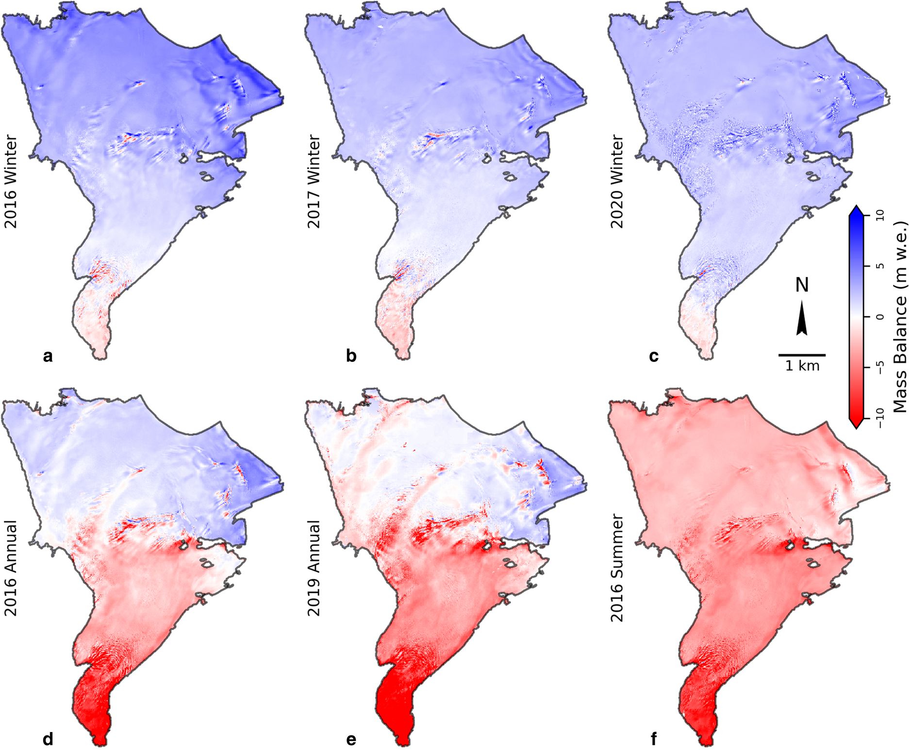
Distributed mass-balance calculations using both profile and GPR emergence velocity constraints gave realistic distributions of mass balance in all six time periods (Figs 5, S9). Strong elevation-dependent trends along with elevation-independent spatial variability are evident. The patterns in spatial variability are consistent across years (Figs 5, S9) and align with end-of-summer distributions of firn and ice (indicating areas of net ablation) in the accumulation zone (Fig. S10).
Distributed mass balances of the winter (a–c), annual (d, e) and summer (f) periods between the DEM survey dates (Table 1), calculated using GPR emergence velocities. Winter mass loss near the terminus in a–c is due to melt which occurred after the fall DEM surveys and before snow began accumulating.
7. Discussion
7.1. Comparison with in situ mass balances
Comparison between distributed mass balances and in situ mass-balance measurements at stakes (by extracting the pixel value of the distributed mass-balance product at each stake location) showed good agreement when using both profile and GPR emergence velocity products (Fig. 6). Using the GPR emergence was more accurate than the profile emergence constraints (RMSE of 0.62 vs 0.73 m w.e., r = 0.99 for both, n = 41) and less biased (−0.23 vs − 0.47 m w.e.; Table 2). Results tended to be more accurate over seasonal than annual time frames (Table 2).
Comparison of in situ stake mass-balance measurements and distributed mass balances. (a) The distributed mass balances using the GPR emergence constraints, and (b) results using the profile emergence. Statistics are presented in Table 2.

RMSE, mean bias (stake minus distributed) and Pearson correlation coefficient (r) for the comparison between distributed and stake mass-balance measurements, using both GPR and profile emergence constraints. Statistics are presented for all 41 observations, as well as subset into winter, summer and annual time periods. ‘Obs’ indicates the number of stake measurements for each time period. RMSE and bias are in units of m w.e.

Further comparison between GPR-derived snow depths converted to snow-water equivalent (SWE) using measured snow densities (McGrath and others, Reference McGrath2018) and winter-distributed mass balances revealed stronger agreement than stake comparisons (Table 3). The mass-balance model and stake-measured winter ablation were used to account for melt which occurred after the fall DEM in each year, such that the balance maps showed the SWE contained in snow on the date of the GPR surveys. Average RMSE of the three years were similar when using GPR and profile emergence constraints (0.35 and 0.38 m w.e.), with the RMSE of individual winters ranging from 0.32 to 0.41 m w.e. Correlation coefficients ranged from 0.69 to 0.95, with a mean of 0.85. Overall, the use of GPR emergence velocities gave less biased results than profile emergence constraints, with the magnitude of bias not exceeding 0.27 m w.e. in any year. Further comparisons between emergence constraints, individual years and differences between the accumulation and ablation zone can be found in Table 3.
Statistics for the distributed-minus-GPR winter balance comparisons (Fig. 7) showing the mean bias (distributed minus GPR), RMSE and Pearson correlation coefficient (r) of the differences over the entire glacier surface as well as for only the accumulation and ablation zones. Obs refers to the number of 10 m × 10 m grid cells observed each year. RMSE and bias are in units of m w.e.

Comparison of GPR measured winter mass balances with distributed mass balances, using GPR emergence (a, b, e, f, i, j) and profile emergence (c, d, g, h, k, l) in the three winters as shown by the labeled years on the left. Maps display the spatial distribution of differences (distributed minus GPR). Scatterplots compare the mass balances at each point to each other, displayed as a heatmap. Dashed blue lines indicate the line of perfect agreement between the two datasets. Statistics are presented in Table 3.

Glacier-wide average mass balance from the distributed mass-balance fields were compared to geodetically calibrated glaciological measurements (Fig. 8, Table S3; O'Neel and others, Reference O'Neel2019). Absolute differences were <0.87 m w.e. (RMSE = 0.47 m w.e., r = 0.98). The two mass-balance approaches gave very similar results across all seasonal and annual time periods, with maximum differences of 0.29 m w.e. (Fig. 8).
Glacier-wide balances, using both GPR and profile emergence constraints, compared to glaciological glacier-wide balances. W, A and S refer to winter, annual and summer balances of the respective year. Distributed balances were temporally aligned to the glaciological mass-balance dates using the mass-balance model. Black lines indicate error estimates. Errors for glaciological seasonal balances were not estimated.

Balance profiles were calculated from our distributed mass-balance maps using the mean for each 100 m elevation band on the glacier surface. Profiles calculated using GPR and profile emergence velocity constraints showed good agreement over the majority of the glacier surface, diverging most in the lowest 300–400 m near the terminus (Fig. 9). These profiles were compared to balance profiles constructed from stake observations (O'Neel and others, Reference O'Neel2019). Differences between the distributed and stake-derived profiles tended to be greatest at the profile tails (which contain only a small proportion of the total glacier area) where stake-derived profiles are linearly extrapolated beyond observations and where emergence velocities are more variable and less well constrained (Fig. 9).
Balance profiles from stake data (black lines), and balance profiles from distributed mass-balance maps in 100 m elevation bands using GPR (blue) and profile (red) emergence constraints. Filled blue and red areas indicate the interquartile range of pixel values within each elevation band. Note varying y-axis limits.

7.2. Emergence velocity measurements
The three methods presented for measuring emergence velocities produced consistent results (Fig. 3), but each give varying spatial and temporal resolution of the glacier-wide emergence field. GPR emergence velocities offer high spatial resolution snapshots of the emergence velocities across the entire glacier surface. However, they can only be measured over the winter (when minimal ablation occurs) and as such cannot capture seasonal variations and may introduce bias when used over summer or annual time periods. Alternatively, profile emergence velocities offer elevation profiles of emergence velocity averaged over multiple years, which are likely to be less prone to seasonal biases but do not reveal seasonal patterns or the same spatial resolution as GPR emergence products. Stake emergence velocities offer sparse point observations of emergence velocities on sub-seasonal to annual time frames, with the potential to track multi-year to decadal patterns. However, they do not reveal the same level of spatial coverage that can be derived from GPR or profile emergence products.
Although variability in stake emergence velocities was observed in most mass-balance stakes in this study, the largest variability was found at stakes closest to the terminus in both the historical and modern stake datasets (Figs 3, S5). This observation is in line with previous studies on mountain glaciers in western Canada (Beedle and others, Reference Beedle, Menounos and Wheate2014) and the French Alps (Vincent and others, Reference Vincent2021), where significant inter-annual and spatial variability was observed in dense stake networks (n ≈ 20) near each glacier's terminus. A year-long investigation of emergence velocities at five stakes in the slow-flowing (~10 m a−1) accumulation zone of a glacier in the French Alps found no significant temporal variability at monthly timescales, yet significant spatial variability (Réveillet and others, Reference Réveillet2021).
A long-term stake array spanning the entire elevation range of Kesselwandferner, Austria (Stocker-Waldhuber and others, Reference Stocker-Waldhuber, Fischer, Helfricht and Kuhn2019) captured inter-annual variability in emergence between 1965 and 1985 similar in magnitude to those observed on Wolverine Glacier. Over this time period Kesselwandferner was advancing and had comparable horizontal ice flow velocities to Wolverine Glacier. However, emergence velocities have been more stable on Kesselwandferner since 1985, during which time the glacier has been retreating and exhibited decreased horizontal flow velocities.
No significant correlation between individual measurements of horizontal velocities and emergence velocities of stakes on Wolverine Glacier was observed (R 2 < 0.1 in all historical stakes, R 2 < 0.3 in modern stakes; Fig. S11), except for modern stake AU where rapid simultaneous decreases in horizontal and emergence velocities were seen (Fig. S6). This suggests that although general seasonal patterns may be apparent (Fig. S7), individual seasonal to annual variations in measured horizontal velocities cannot be assumed to lead directly to changes in the magnitude of emergence. However, over longer time periods this seems to be the case (as observed in Stocker-Waldhuber and others, Reference Stocker-Waldhuber, Fischer, Helfricht and Kuhn2019).
The small-scale spatial variability in emergence velocities observed in these studies (Beedle and others, Reference Beedle, Menounos and Wheate2014; Réveillet and others, Reference Réveillet2021; Vincent and others, Reference Vincent2021) suggests that rapidly changing glacier geometry, temporal variability in mass-balance distributions, inherent small-scale spatial variability in the emergence field and uncertainties in the measurements all contribute to measured variability in the emergence at a given stake. The variability observed here shows that caution should be used when extrapolating sparse stake emergence velocity measurements across larger spatial and temporal scales.
7.3. Dynamic terminus characteristics
A consistent observation in the emergence velocities and distributed mass-balance measurements is that the terminus of Wolverine Glacier shows behaviors that are distinct from the upper glacier and is undergoing dynamic changes. Seasonal variations in emergence observed in the stake data (Fig. S7) were most pronounced at the terminus, where occasional summer submerging flow was estimated. The greater magnitude of seasonality in emergence is consistent with the more pronounced seasonality in horizontal velocities for lower elevation regions of the glacier in both the historical and modern stake datasets (Fig. S8). However, horizontal velocities and emergence velocities near the terminus vary inversely, with the greatest emergence occurring in the mid-winter when the horizontal velocities are at their lowest.
Wolverine Glacier is undergoing a dynamic response to recent mass loss, as evidenced by the declining magnitude of emergence near the terminus relative to the rest of the ablation zone that is captured in the GPR and profile emergence velocities (Figs 3, S3) and decreasing horizontal velocities (from 35 to 10 m a−1) and emergence velocities (from 5 to 0 m a−1) over the past decade (Fig. S6). Ice melt near the terminus is outpacing the rate of ice influx, leaving the remaining ice dynamically disconnected from the upper glacier, and leading to more rapid thinning of the terminus than the rest of the glacier. Similar patterns in glacier retreat and emergence were observed on Kesselwandferner (Stocker-Waldhuber and others, Reference Stocker-Waldhuber, Fischer, Helfricht and Kuhn2019), with the horizontal velocities and emergence velocities of the lowest elevation stake decreasing over time before eventually being lost to ice melt and glacier retreat. Decreasing magnitudes of emergence near the terminus of Findelengletscher were found using the same profile approach that is employed in this study (Sold and others, Reference Sold2013).
This pattern of decreasing emergence was observed on Wolverine Glacier in both the 2008–12 and 2015–19 profile emergence products, with a sharper inflection seen in the more recent period. The pattern was not seen in earlier periods (1972–79, 1972–95), suggesting it is a recent development. Findings from previous studies of emergence velocities which focus on areas near their respective glaciers’ termini may not be applicable to other areas of those glaciers, or in future years if the emergence field undergoes significant changes.
The dynamic nature of Wolverine Glacier's lowest elevations, in conjunction with limited stake and GPR observations, makes accurate measurements of short-interval distributed mass balances more difficult. Emergence magnitudes and distributions vary from year-to-year more than they do over the rest of the glacier and uncertainties in these values are greater (Fig. 3). More detailed investigation of the spatiotemporal patterns in this area, in the context of the wider glacier dynamics, is needed to provide more reliable short-term distributed mass-balance measurements of the terminus. Such investigations could include: detailed GPR surveys to better constrain snow depths, and repeat LiDAR surveys over short temporal scales to identify fine resolution patterns of ablation.
7.4. Insights on mass-balance processes
The distributed mass-balance maps and balance profiles derived from them (Fig. 9) allow insights into mass-balance processes that are not detectable with sparse stake networks. Previous studies have examined the spatial distribution of accumulation on Wolverine Glacier and other glaciers in detail using a variety of approaches (Sold and others, Reference Sold2013; McGrath and others, Reference McGrath2015), but observations of ablation patterns have remained limited. Here we show that ablation and accumulation have fundamentally different spatial distributions which both exert control on the annual mass-balance distribution, and they particularly diverge in areas of complex topography such as icefalls.
Winter balance profiles show consistently increasing mass balances with elevation (Figs 9a–c), suggesting that balance profiles can give reasonable estimates of the elevation-distribution of snow accumulation at Wolverine Glacier (given accurate measurements across the elevation range of the glacier). Conversely, summer and annual balances show variations from these linear increases at 900 and 1200 m a.s.l. (Figs 9d–f). The locations of these areas of increased ablation rates align with two icefalls: one at the border between the accumulation and ablation zone, and the other at the transition from the flat and smooth upper ablation area (~ 900–1200 m a.s.l.) to the lower and rougher icefall. This highlights the important roles that surface slope, roughness and albedo play in controlling ablation rates. Surface roughness in these heavily crevassed areas increases ablation rates via the alteration of turbulent heat fluxes and increased surface area over which ablation can occur (Colgan and others, Reference Colgan2016), while decreased albedo causes an increase in absorbed shortwave radiation and thus amount of energy available for melt (Braithwaite, Reference Braithwaite1995). The convex nature of icefalls can result in areas of decreased accumulation in the winter from enhanced wind scour, which in turn exposes lower-albedo ice surface earlier in the summer, increasing the net summer ablation.
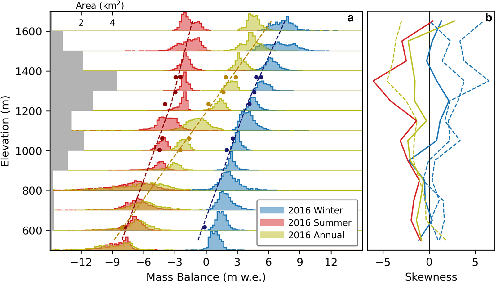
Binned at 100 m, winter mass-balance distributions demonstrate positive skewness whereas summer and annual mass-balance distributions exhibit negative skewness (Fig. 10). Positively skewed winter balances are the result of areas of snow accumulation which are greater than the elevation-mean (i.e. drifted areas) being more common than areas less than the elevation-mean (i.e. scoured areas). The negatively skewed summer balances highlight higher ablation rates relative to the elevation-mean, such as the icefalls and other crevassed areas with greater surface roughness and associated turbulent heat fluxes (Fitzpatrick and others, Reference Fitzpatrick, Radić and Menounos2017). The negative skewness of annual balances suggests that ablation patterns are ultimately more influential than accumulation patterns in determining annual balance distributions.
(a) Annual, summer and winter distributed mass-balance histograms for 2016, from 10 m × 10 m pixels binned within 100 m bands. Histograms are normalized and represent only the relative distribution of balances. Dots show stake-measured mass balances and the corresponding balance profile (dashed lines) from these points. Distributed mass balances were calculated using profile emergence constraints and have been temporally aligned with the dates of the stakes and balance profiles. (b) Skewness of the balance distribution within each band, with colors corresponding to winter (blue), summer (red) and annual (yellow) time periods. Solid lines correspond to the 2016 observations, shown in (a), and dashed lines are for other time periods (histograms shown in Figs S12, S13).
Objective hazards typically limit the placement of mass-balance stakes to the more topographically smooth terrain on mountain glaciers. This preferential placement will tend to positively bias the measured summer balances by avoiding crevassed zones, where increased ablation rates occur. Similarly, winter balances may be negatively biased by avoiding these same areas where deeper snow depths can occur. At Wolverine Glacier these biases in summer measurements are more significant than the biases in winter measurements, as shown by the tendency for annual glaciological balances to underestimate mass loss compared to decadal-scale geodetic reanalyses (O'Neel and others, Reference O'Neel2019).
The distributed mass-balance products (Fig. 5) were used to identify locations which tend to capture the average mass-balance changes of their respective elevation (Fig. 11). Only 3% of the glacier surface was within either 5% or 0.2 m w.e. of the mean balance of the surrounding 100 m elevation band in all six balance periods (Fig. 11d). There are no areas at the elevations containing the upper icefall, lower icefall or below the lower icefall. These patterns illustrate the conundrum of in situ mass-balance networks. Areas of relatively simple topography have stable seasonal to annual balance patterns which are able to be captured by well-placed mass-balance stakes. However, these areas tend to be associated with more positive mass balances than topographically complex areas, so limiting stake placements to those locations could increase the magnitude of geodetic calibrations.
Areas on Wolverine Glacier where summer (a), annual (b) and winter (c) mass balances were within 0.2 m w.e. or 5% of the mean balance of all areas within their respective 100 m elevation band. Open circles show the locations of the current mass-balance stake array. Darker areas in (b) and (c) indicate pixels that were within 0.2 m w.e. or 5% for multiple years (i.e. both annual years, and two or three winters). (d) Pixels which were within 0.2 m w.e. or 5% of their elevation band in all six mass-balance periods, indicating that they are more likely to accurately capture the average mass-balance changes of their respective elevations over summer, winter and annual time frames.

Topographically complex areas, which tend to have more negative balances, are difficult to measure with mass-balance stakes due to divergent patterns of accumulation and ablation. Furthermore, inter-annual changes in glacier geometry in these regions introduces year-to-year variability in mass-balance distributions, confounding the inter-annual changes which stakes are meant to measure. A similar problem is encountered in the area below the lower icefall (near AU, the lowest elevation stake). Because the lower glacier is stagnating and thinning rapidly, the surface geometry is changing at a similarly rapid rate. This introduces inter-annual variations in accumulation and ablation patterns which preclude a consistently placed stake from capturing the representative mass balance of the area over the course of multiple years.
Placing a stake at the same elevation as an icefall but in a less topographically complex area (such as stake S, the eastern-most stake) will not necessarily capture the average mass-balance of that elevation, and as such may give false confidence in the ability to constrain those mass changes. The areas highlighted in Figure 11 should be interpreted only as capturing the balance patterns of their respective elevations; they cannot reveal the mass-balance changes at other elevations. Fitting an elevation-dependent balance profile between these points to extrapolate glacier-wide mass balance would still give biased results in the icefalls and lower glacier areas.
These issues illustrate why even dense in situ networks tend to require geodetic calibration over decadal timescales (Zemp and others, Reference Zemp2013; Klug and others, Reference Klug2018; O'Neel and others, Reference O'Neel2019). While they may not allow unbiased absolute mass change estimates, the value of in situ programs lies in their ability to provide validation and calibration of geodetic surveys, annual to sub-annual temporal variability and process-based insights in glacier mass balance that would otherwise not be observable.
8. Conclusions
This study on a relatively data-rich glacier shows how geodetic products and in situ observations can be leveraged on fine spatiotemporal scales to gain detailed insights on mass-balance processes. We used a mass continuity approach to derive spatially resolved seasonal and annual distributed mass balances of Wolverine Glacier. Point comparisons of these distributed balances showed good agreement when compared with mass-balance stakes (RMSE = 0.67 m w.e., r = 0.99, n = 41), end-of-winter GPR-derived snow depths (RMSE = 0.36 m w.e., r = 0.85, n = 9024) and geodetically calibrated glacier-wide mass balances (RMSE = 0.47 m w.e., r = 0.98, n = 6).
Key differences revealed by three emergence velocity measurement methods suggest that small-scale spatiotemporal variations (seasonal and 10–100 m) in ice flow have important implications for the precision of measured mass-balance distributions, particularly in areas undergoing dynamic changes such as a thinning and retreating terminus. Caution should be used when spatially and temporally extrapolating limited point measurements of emergence velocities.
Stake-derived balance profiles tend to diverge the most from distributed estimates in areas where measurements are limited: at the highest elevations, lowest elevations and in heavily crevassed icefalls. Anomalously high ablation rates were found in icefalls, showing how physical factors other than elevation (surface roughness and albedo) play important roles in governing ablation rates in these areas. We observed positively skewed winter balance distributions and negatively skewed summer and annual balance distributions when controlling for elevation (Fig. 10), reflecting the distinct processes that govern spatial patterns in accumulation and ablation.
Only 3% of the glacier surface area was found to capture the average mass balance of its respective elevation band in all six mass-balance periods investigated. Those regions were all topographically simple areas of the glacier, while no such areas were found in the more complex regions near the terminus or in elevations associated with icefalls. Topographic complexity causes increased ablation, more divergent pattern of ablation and accumulation and temporal variability of mass-balance spatial patterns. Conventional glaciological methods are unlikely to reliably constrain the mass balances of these regions. This illustrates a fundamental limitation of in situ mass-balance measurements, shows why glaciological mass balances tend to require geodetic calibrations and offers physical explanations for the underestimation of mass loss in some glaciological observations.
The distributed mass balances offer insights into seasonal mass-balance processes that are not detectable with sparse stake networks or remotely sensed products alone. This highlights the value of long-term glaciological mass-balance observations: to provide data which are both complementary and independent of remote-sensing observations, and to facilitate integrated approaches to studying mountain glaciers.
Supplementary material
The supplementary material for this article can be found at https://doi.org/10.1017/jog.2022.46.
Data availability
All data used in this analysis are publicly available. Point mass-balance observations, glaciological seasonal and annual balances, stake GNSS data, firn density profiles, meteorological data and most geodetic surveys are available through the USGS (https://doi.org/10.5066/F7HD7SRF). Three DEMs (05/07/2016, 09/10/2016 and 9/20/2019) are available via CRREL's http://lidar.io archive. Derived products from this analysis (distributed mass balances, emergence velocities, firn compaction rates and co-registered 10 m resolution DEMs) can be found at https://doi.org/10.5281/zenodo.6126663. Analytical scripts are available from Lucas Zeller upon request.
Acknowledgements
This work was funded by the U.S. Geological Survey, Cooperative Ecosystems Studies Unit Agreement G19AC00166. LiDAR data collection and processing was contributed by the Remote Sensing/Geographic Information Systems Center, US Army Corps of Engineers Cold Regions Research and Engineering Laboratory (CRREL). Any use of trade, firm or product names is for descriptive purposes only and does not imply endorsement by the U.S. Government. Thank you to Michael Zemp and three anonymous reviewers whose insightful comments improved the quality of the paper.
Author contributions
Concept and design were done by DM, LS, LZ, SO; programming by LZ, CM, LS, DM; formal analyses by LZ; data curation by EB, CM; writing by LZ; edit and review by LZ, DM, LS, SO, CM, EB; visualization by LZ; funding acquisition and project administration by SO, DM, LS.


 Open access