2. GLEAM observing, imaging, and source finding

We refer the reader to Wayth et al. (Reference Wayth2015) and Hurley-Walker et al. (Reference Hurley-Walker2017) for details of the survey strategy and data reduction methods for the GLEAM year 1 extragalactic catalogue, respectively. In this section, we highlight the points salient to this paper.

The GLEAM survey was conducted using Phase 1 of the MWA, which consisted of 128 16-crossed-pair-dipole tiles, distributed over an area ≈3 km in diameter. The whole sky south of Dec +30º was surveyed using meridian drift scan observations. The sky was divided into seven declination strips and one declination strip was covered in a given night. The observing was broken into a series of 2-min scans in five frequency bands (72–103, 103–134, 139–170, 170–200, and 200–231 MHz), cycling through the five frequency bands in 10 min.

Each 2-min snapshot observation was imaged separately using wsclean (Offringa et al. Reference Offringa2014), a w-stacking deconvolution algorithm which appropriately handles the w term for widefield imaging. For imaging purposes, the 30.72-MHz bandwidth was split into four 7.68-MHz sub-bands. The final image products consist of 20 Stokes I 7.68-MHz sub-band mosaics spanning 72–231 MHz as well as four deep wide-band mosaics covering 170–231, 139–170, 103–134, and 72–103 MHz, formed by combining the 7.68-MHz sub-band mosaics.

The source finder aegean (Hancock et al. Reference Hancock2012; Hancock, Trott, & Hurley-Walker Reference Hancock, Trott and Hurley-Walker2018) was run on the 170–231 MHz image to create a blind source catalogue centred at 200 MHz. The catalogue was filtered to exclude areas within 10º of the Galactic plane and other areas affected by poor ionospheric conditions or containing bright, extended sources such as Centaurus A (see Table 1 for details). The filtered catalogue covers an area of 24 831 deg², hereafter referred to as region A, and contains 307 455 components above 5σ, where σ is the rms noise. It is estimated to be 90% complete at S _{200 MHz} = 170 mJy. In order to provide spectral information across the full frequency range, the priorised fitting mode of aegean was used to perform flux density estimates across the 20 7.68-MHz sub-bands. The catalogue provides both peak and integrated flux densities. The peak flux densities were corrected for ionospheric smearing as outlined below. The three lowest frequency wide-band images were not used to provide measurements for the catalogue.

Table 1.

Summary of sky regions excised from the GLEAM survey used in the analyses of this paper.

The top row indicates the total surveyed area in GLEAM. The GLEAM catalogue area covers 24 831 deg² and consists of the total surveyed area excluding the regions listed in the middle rows. The peeled sources are Hydra A, Pictor A, Hercules A, Virgo A, Crab, Cygnus A, and Cassiopeia A; their positions are listed in Hurley-Walker et al. (Reference Hurley-Walker2017).

The GLEAM flux densities are tied to the flux density scale of Baars et al. (Reference Baars, Genzel, Pauliny-Toth and Witzel1977). Overall, the GLEAM catalogue is consistent with Baars et al. to within 8% for 90% of the survey area, where the difference is primarily caused by uncertainty in the MWA primary beam model.

2.1. Correcting peak flux densities for ionospheric smearing

Ionospheric perturbations cause sources to be smeared out in the final, mosaicked images. The magnitude of the effect is proportional to v ⁻², where v is the frequency. Consequently, at any map position, the actual point spread function (PSF) is larger than the restoring beam by a certain amount, depending on the degree of ionospheric smearing. Hurley-Walker et al. (Reference Hurley-Walker2017) used sources known to be unresolved in higher resolution radio surveys to sample the shape of the PSF across each of the mosaics. Maps of the variation of a _psf, b _psf, and pa _psf were produced, where a _psf, b _psf, and pa _psf are the major and minor axes and position angle of the PSF, respectively.

The increase in area of the PSF resulting from ionospheric smearing is given by

\begin{equation}R = {{{a_{{\rm{PSF}}}}{b_{{\rm{PSF}}}}} \over {{a_{{\rm{rst}}}}{b_{{\rm{rst}}}}}},\end{equation}(1)

where a _rst and b _rst are the major and minor axes of the restoring beam, respectively. Sources detected in the 170–231 MHz image have a mean value of R of 1.14, with a standard deviation of 0.04, and in regions worst affected by ionospheric smearing, R reaches 1.44. Ionospheric smearing not only increases the source area by a factor of R but also reduces the peak flux density by the same amount, while integrated flux densities are preserved. In order to restore the peak flux density of the sources, the images were multiplied by R. In the catalogue, integrated flux densities were normalised with respect to the position-dependent PSF to ensure that, for bright point sources, peak and integrated flux densities agree.

3. Source finding at 154, 118, and 88 MHz

Since a statistically complete sample is required to measure the counts at any frequency, we cannot use the sub-band measurements quoted in the GLEAM catalogue, obtained from the priorised fitting, to measure the counts. In order to derive the counts at frequencies below 200 MHz, we use the wide-band images covering 139–170, 103–134, and 72–103 MHz, centred at 154, 118, and 88 MHz, respectively.

We create a blind source catalogue at each of these frequencies following a similar procedure to that employed by Hurley-Walker et al. (Reference Hurley-Walker2017). We first use bane (Hancock et al. Reference Hancock, Trott and Hurley-Walker2018) to remove the background structure and estimate the rms noise across the image. The ‘box’ parameter defining the angular scale on which the rms and background are evaluated is set to 20 times the synthesised beam size. We then run the source finder aegean using a 5σ detection threshold. The integrated flux densities are normalised using the PSF map at the relevant frequency. Sources lying within areas flagged from the GLEAM catalogue (see Table 1) are excluded. The number of sources detected at each frequency and other source-finding statistics are given in Table 2.

Table 2.

Source-finding statistics in region A, covering 24 831 deg². For the 5σ detection threshold, and PSF major and minor axes, we quote the mean and standard deviation. Sources are classified as extended as described in Section 4.1.

The mosaics used to create the source catalogues have a relatively large fractional bandwidth; the 88-MHz mosaic has the largest fractional bandwidth of ≈0.35. For any source with a non-zero spectral index, there is a discrepancy between the average flux density integrated over the band, S _w, and the monochromatic flux density, S ₀, at the central frequency, v ₀, for two reasons. Firstly, most sources are better described by a power–law slope across the band than a simple linear slope. S _w will always exceed S ₀ for a source with a power–law slope. The magnitude of this effect increases with fractional bandwidth and for a source with an increasingly nonflat spectrum. The second cause of the discrepancy is the inverse noise-squared weighting applied to the 7.68-MHz sub-band mosaics: in practice, the noise in the 7.68-MHz sub-band mosaics decreases slightly with frequency, causing more weight to be assigned to higher frequency mosaics. For a source with α < 0, where α is the spectral index (S ∝ v ^α), these two effects go in opposite directions: S _w increases as a result of the power–law slope of sources across the band and decreases as a result of the weighting scheme adopted in the mosaicking.

For sources detected in each of the wide-band mosaics, we calculate the required flux density correction factor, S ₀/S _w. At any position in the mosaic,

\begin{equation}{S_{\rm{w}}} = \Sigma _{i = 1}^N{w_i}{S_0}{\left( {{{{\nu _i}} \over {{\nu _0}}}} \right)^\alpha },\end{equation}(2)

where w_i is the weight assigned to the ith sub-band, normalised such that $ \Sigma _{i = 1}^N{w_i} = 1.0 $, v_i is the central frequency of the ith sub-band, and N is the number of 7.68 MHz sub-bands. The flux density correction factor is given by

\begin{equation}{{{S_0}} \over {{S_{\rm{w}}}}} = {\left[ {\Sigma _{i = 1}^N{w_i}{{\left( {{{{\nu _i}} \over {{\nu _0}}}} \right)}^\alpha }} \right]^{ - 1}}.\end{equation}(3)

We produce simulated images of the flux density correction factor using the mosaicking software swarp (Bertin et al. Reference Bertin, Mellier, Radovich, Missonnier, Didelon, Morin, Bohlender, Durand and Handley2002) assuming α = −0.8, the typical spectral index of GLEAM sources between 76 and 227 MHz. Using these images we extract the correction factor for sources detected in each of the wide-band images. We find that the mean ± standard deviation of the correction factor in the 200, 154, 118, and 88 MHz mosaics is 1.000 ± 0.009, 1.003 ± 0.001, 1.007 ± 0.002, and 1.002 ± 0.004, respectively. Given the correction factors are very close to unity ( < 1%), we ignore them.

4. Determining the source counts

We measure the source counts at 200 MHz using the wide-band flux densities quoted in the GLEAM catalogue and at 154, 118, and 88 MHz using the catalogues compiled in Section 3. At each frequency, the vast majority of sources are point like due to the large beam size. For unresolved sources, peak flux densities will be significantly more accurate than integrated flux densities at low signal-to-noise ratio (SNR). This is because more free parameters are required to measure an integrated flux density using Gaussian fitting. We note that peak flux densities are corrected for ionospheric smearing as outlined in Section 2.1. Therefore, in measuring the counts, we only use integrated flux densities for sources which are significantly resolved and use peak flux densities for the remaining sources. We distinguish between point-like and extended sources as described in Section 4.1.

The rms noise varies substantially across the survey due to varying observational data quality and the presence of image artefacts originating from bright sources and the Galactic Plane. It increases at lower frequency and becomes less Gaussian as the classical confusion noise becomes more dominant. The counts must be corrected for both incompleteness and Eddington bias (Eddington Reference Eddington1913) close to the survey detection limit. Incompleteness causes the counts to be underestimated close to the detection limit, while the Eddington bias makes it more likely for noise to scatter sources above the detection limit than to scatter them below it due to the steepness of source counts, consequently boosting the counts in the faintest bins. The magnitude of the Eddington bias only depends on the SNR and the source count slope (Hogg & Turner Reference Hogg and Turner1998).

The number of synthesised beams per source is often used as a measure of confusion as it indicates the typical separation of sources at the survey cut-off limit. The number of beams per source at each frequency is indicated in Table 2. It is only 24 at the lowest frequency, indicating that the average separation between sources is $ \sqrt {24} \approx 5 $ beams. Vernstrom et al. (Reference Vernstrom, Scott, Wall, Condon, Cotton and Perley2016) used simulated images to investigate the effect of confusion on the source-fitting accuracy for the source finders aegean and obit (Cotton Reference Cotton2008). Similar results were obtained for both source finders: sources separated by less than the beam size were fitted as a single source up to 95% of the time, while the total flux density of the sources was, on average, conserved. Thus the effect of confusion is either to prevent a source from being detected or to boost its flux density, which may, in turn, significantly bias the counts. In Section 4.2, we use Monte Carlo simulations to investigate the effect of incompleteness, Eddington bias, and source blending on the counts.

Conversely, sources (i.e. physical entities associated with a host galaxy) of largest angular size may also be broken up into multiple components in GLEAM. In measuring the source counts, physically related components should be counted as a single source and their flux densities summed together. In Section 4.3, we show that, given the large beam size, the source counts are well approximated as counts of components.

4.1. Classifying sources as point-like or extended

We use the method described in Franzen et al. (Reference Franzen2015) to identify extended sources based on the ratio of integrated flux density, S, to peak flux density S _peak. Assuming that the uncertainties on S and S _peak (σ _S and σ _{S peak} respectively) are independent, to detect source extension at the 2σ level, we require

\begin{equation}\ln \left( {{S \over {{S_{{\rm{peak}}}}}}} \right) \gt 2\sqrt {{{\left( {{{{\sigma _{\rm{S}}}} \over S}} \right)}^2} + {{\left( {{{{\sigma _{{S_{{\rm{peak}}}}}}} \over {{S_{{\rm{peak}}}}}}} \right)}^2}} \;.\end{equation}(4)

We take σ _{S peak} and σ _S as the sum in quadrature of the Gaussian parameter fitting uncertainties returned by aegean, which accounts for the local noise, and the GLEAM internal flux density calibration error. The latter is estimated to be 2% at −72º ≤ Dec < 18.5º and 3% at Dec < −72º and Dec ≥ 18.5º (Hurley-Walker et al. Reference Hurley-Walker2017). For bright sources, where the 2% calibration error dominates, $ {S \over {{S_{{\rm{peak}}}}}} \lt 1.06 $ is considered to be extended.

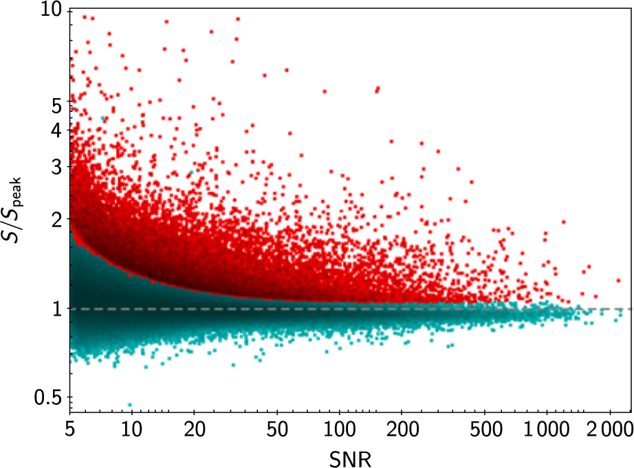
Table 2 gives the fraction of sources classified as extended at each frequency. Figure 1 shows $ {S \over {{S_{{\rm{peak}}}}}} $ as a function of SNR for all sources detected at 200 MHz. 7.3% of sources are classified as extended at this frequency, where the beam size (≈2.5 arcmin) is smallest; these are highlighted in red.

Figure 1.

S/S _peak as a function of SNR for all components detected at 200 MHz. The peak flux density values have been corrected for ionospheric smearing as described in Section 2.1. Components which are classified as point-like/extended are shown in turquoise/red.

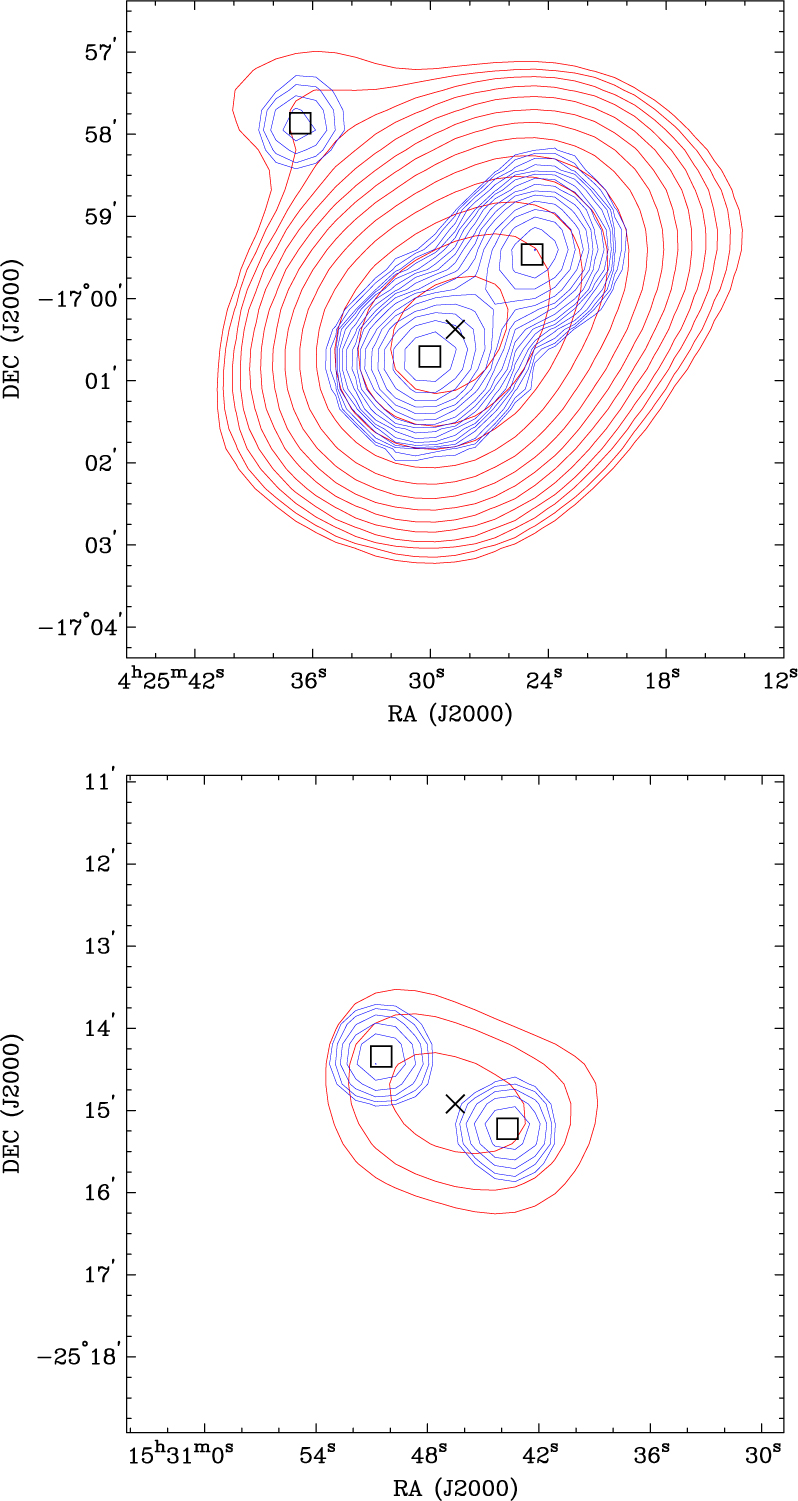
Investigations using higher resolution (45 arcsec) radio images from the NRAO VLA Sky Survey (NVSS; Condon et al. Reference Condon, Cotton, Greisen, Yin, Perley, Taylor and Broderick1998) at 1.4 GHz show that a large fraction of resolved sources in GLEAM are, in fact, artefacts of source confusion or noise fluctuations: we randomly select 50 sources classified as extended at 200 MHz in the region of sky covered by NVSS, i.e. at Dec > −40º. We find that 39 of the sources are resolved into multiple components in NVSS. Of these 39 sources, only 16 are likely to be genuinely extended because the NVSS components have similar peak flux densities and there is extended emission linking the components; the remaining 23 sources probably appear extended as a result of source blending. An example of each of these cases is shown in Figure 2.

Figure 2.

An example of an extended GLEAM source associated with a resolved NVSS double (top) and with two NVSS components determined to be unrelated (bottom). Red (GLEAM) and blue (NVSS) contours are shown with the lowest contour level at 3σ; the contour levels increase at each level by a factor of $ \sqrt 2 $. GLEAM and NVSS component positions are represented as crosses and squares, respectively.

4.2. Correcting the counts for incompleteness, Eddington bias, and source blending

We conduct Monte Carlo simulations to quantify the effect of incompleteness, Eddington bias, and source blending on the counts. Our approach is to inject synthetic point sources with a range of flux densities into the wide-band images using aeres from the aegean package. We then use exactly the same source-finding procedure as described in Section 3 to detect the simulated sources and measure their flux densities. The corrections to the counts as a function of flux density are obtained from the ratio of the injected count to the measured count of the simulated sources.

The major and minor axes of the simulated sources are set to a _psf and b _psf, respectively, which are obtained from the PSF map at the relevant frequency. The simulated sources lie at random positions within region A but we set a minimum separation of 20 arcmin (≈4 times the beam size at the lowest frequency) between simulated sources to avoid them affecting each other. A simulated source may lie too close to a real (>5σ) source to be detected separately. In such situations, if the recovered source is closer to the simulated source than the real source, the simulated source is considered to be detected, otherwise not. Thus we account for source confusion in the counts in this analysis.

It is important to ensure that the flux density distribution of the simulated sources is as realistic as possible and extends to well below the 5σ detection limit (≳ 50 mJy/beam at 154 MHz). This is because the Eddington bias is dependent on the slope of the counts and causes the flux densities of sources with low SNRs to be biased high, boosting the number of sources detected in the faintest bins. The flux density distribution of the simulated sources at 154 MHz is based on the following source count model: above 33 mJy, we use a third-order polynomial fit to 154-MHz counts from a 12-h pointed MWA observation of an EoR field, covering 570 deg² (Franzen et al. Reference Franzen2016). Between 6 and 33 mJy, deep 153-MHz GMRT counts from Williams, Intema, & Röttgering (Reference Williams, Intema and Röttgering2013) and Intema et al. (Reference Intema, van Weeren, Röttgering and Lal2011) are well represented by a power law of slope γ = 0.96, where $ {S^{2.5}}{{{\rm{d}}N} \over {{\rm{d}}S}} = k{S^\gamma } $. We therefore set γ = 0.96 in this flux density range. A total of 40,000 flux densities ranging between 6 mJy and 15 Jy are drawn randomly from the source count model. We extrapolate the simulated source flux densities to 200, 118, and 88 MHz assuming α = −0.8, as indicated by the typical spectral index seen in GLEAM.

The simulations are repeated 40 times to improve statistics. The solid lines in Figure 3 show the mean source counts correction factor in region A, c _A, in each of the wide-band images. The effects of both incompleteness and confusion are clearly evident. The sharp increase in the correction factor at low flux density is due to incompleteness. As expected, the survey becomes incomplete at a higher flux density in the lower frequency images. Source blending causes the correction factor to fall below 1.0 at higher flux densities. At 200 MHz, despite the large beam size of ≈2.5 arcmin, the number of beams per source (49) is low enough for confusion not to strongly affect the counts, which are only overestimated by up to 2–3%. As expected, the effect worsens at lower frequency due to the lower number of beams per source: at 88 MHz, the number of beams per source is 24 and the counts are overestimated by up to 7% as a result of confusion.

Figure 3.

Source count correction factor as a function of flux density at 200 MHz (black), 154 MHz (blue), 118 MHz (purple), and 88 MHz (red). The solid and dashed lines apply to regions A and B, respectively. For clarity, the source count correction factor in region B is only shown below 1 Jy and error bars are not included.

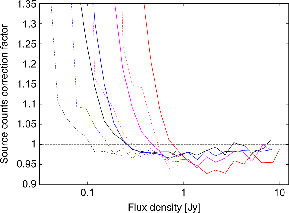
From visual inspection of the rms noise maps, we identify areas within region A where the rms noise is well below average at zenith angles ⪅30º, covering in total 6 516.2 deg². The lines of RA and Dec bounding this region, hereafter referred to as region B, are given in Table 3. The dashed lines show the correction factor in region B, c _B. The counts start becoming incomplete at a flux density about twice as low as in region A at all frequencies. The counts are measured in region A in flux density bins where c _A ≤ 1.2. If c _A > 1.2 and c _B ≤ 1.2, the counts are measured in region B. We do not measure the counts in bins where c _B > 1.2 as the correction factor rises sharply with decreasing flux density in these bins and becomes unreliable.

Table 3.

Region B used to measure the source counts.

4.3. Complex sources

We report counts of components rather than counts for integrated sources. The magnitude of the difference between the two will depend on the beam size and the intrinsic angular source size distribution. S. White et al., in preparation, are analysing a subset of the GLEAM catalogue in detail to study the nature and evolution of the bright end of the low-frequency population. The GLEAM 4 Jy sample is a statistically complete sample of 1 845 sources with S _151MHz > 4.0 Jy, covering region A. Only 44 (2.4%) of the sources are resolved into multiple components, where the beam size is ≈2.5 arcmin. Multi-component sources are identified through visual inspection of higher resolution radio images from NVSS, the Sydney University Molonglo Sky Survey (SUMSS; Bock, Large & Sadler Reference Bock, Large and Sadler1999), and the Faint Images of the Radio Sky at Twenty Centimetres (FIRST; Becker, White, & Helfand Reference Becker, White and Helfand1995) survey. The likelihood of a source showing complex structure increases with flux density above 4 Jy due to the increasing fraction of objects at very low redshifts, as shown in the bottom panel of Figure 4. No multi-component sources are detected in the highest flux density bin (57–114 Jy) but it only contains five sources, three of which are extended in GLEAM and resolved into multiple components in NVSS/SUMSS.

Figure 4.

Top: Euclidean normalised ($ {S^{2.5}}{{{\rm{d}}N} \over {{\rm{d}}S}} $) differential counts of the GLEAM 4 Jy sample at 151 MHz. The red circles show component counts while the black circles show counts for integrated sources. Bottom: fraction of multi-component sources in each flux density bin.

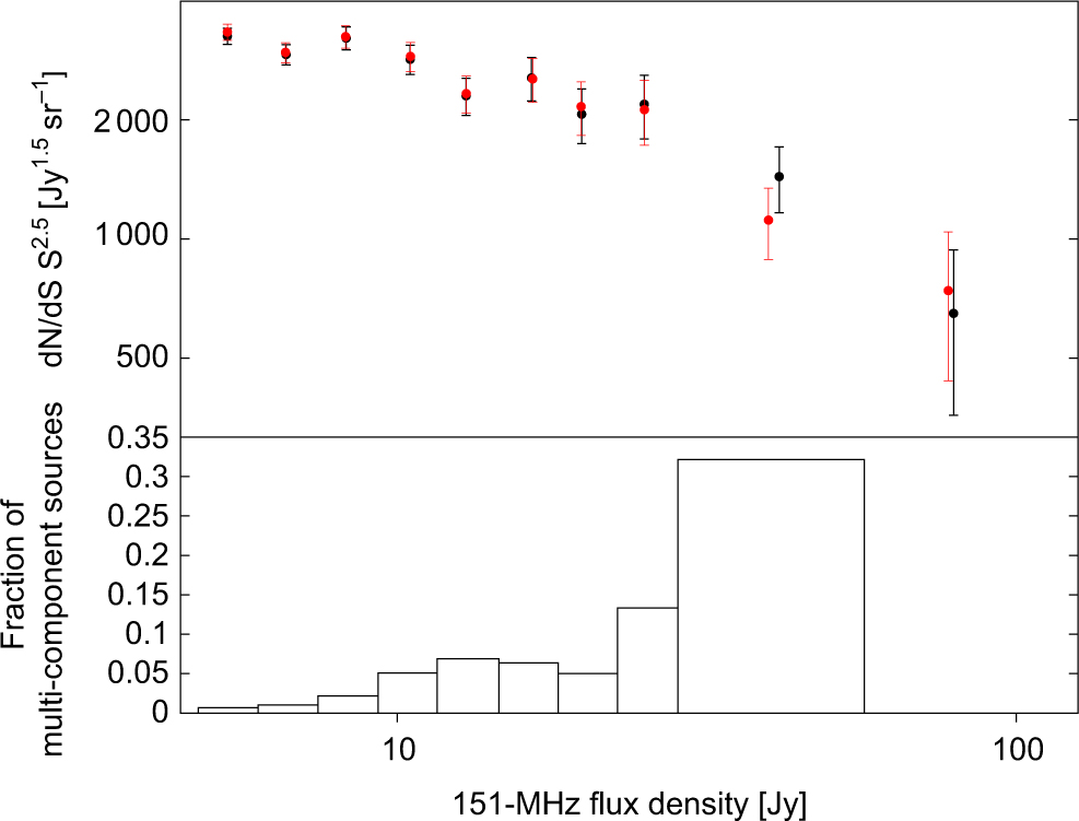
We use the GLEAM 4 Jy sample to measure both the source and component counts at S _151MHz > 4.0 Jy. We find that the component and source counts agree within the Poisson uncertainties, as shown in the top panel of Figure 4, given the small fraction of sources which are resolved into multiple components. Windhorst, Mathis, & Neuschaefer (Reference Windhorst, Mathis and Neuschaefer1990) found that, below S _{1.4 GHz} = 3 Jy, the median angular size of radio galaxies, θ _med, decreases continuously towards fainter flux densities, with θ _med ∝(S _{1.4 GHz})^0.3. Assuming that a similar relation holds at lower frequency, we expect our multi-frequency component counts to be a good approximation of the counts for integrated sources.

Finally, we note that the following bright, complex sources were peeled from the GLEAM data and subsequently lie outside region A: Hydra A, Pictor A, Hercules A, Virgo A, Crab, Cygnus A, and Cassiopeia A. Centaurus A also lies outside region A. From measurements over 60–1 400 MHz available via the NASA/IPAC Extragalactic Database (NED),Footnote ^a these sources are all brighter than 100 Jy at 200, 154, 118, and 88 MHz. Since our highest source count bin does not exceed 100 Jy at any of these frequencies, the exclusion of these sources does not bias our source count measurements.

4.4. Analysis of the GLEAM source counts

The corrected GLEAM differential source counts are shown in Figure 5, while the source count data are provided in Table A1 in Appendix. Uncertainties on the counts are propagated from Poisson errors on the number of sources per bin and the errors on the correction factors derived in Section 4.2. The Poisson error on N is approximated as $ \sqrt N $ in all bins with N ≥ 20. In bins with N < 20, we use approximate expressions for 84% confidence upper and lower limits based on Poisson statistics by Gehrels (Reference Gehrels1986).

Figure 5.

Euclidean normalised differential counts at 200 MHz (black), 154 MHz (blue), 118 MHz (purple), and 88 MHz (red) from GLEAM. The different symbols distinguish between the areas used to derive the counts in the various flux density bins: the filled circles correspond to region A, while the open squares correspond to region B. The solid blue line is a weighted least squares fifth-order polyomial fit to the 154-MHz counts.

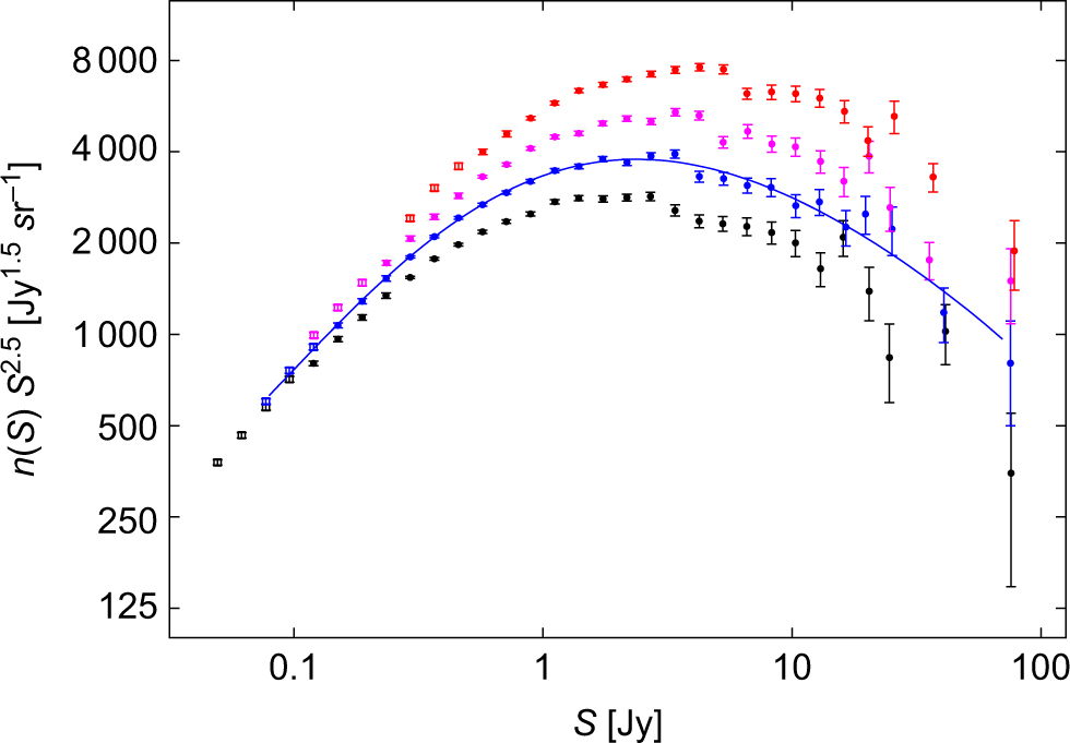
The bulge due to source evolution is clearly evident at all four frequencies given the large areal sky coverage and the range of flux densities sampled. A detailed comparison of the shape of the multi-frequency counts is undertaken in Section 5.

In Figure 6, we compare the GLEAM counts with other counts in the literature at a similar frequency covering more than 100 deg²: the 154-MHz counts by Franzen et al. (Reference Franzen2016), 7C counts at 151 MHz by McGilchrist et al. (Reference McGilchrist, Baldwin, Riley, Titterington, Waldram and Warner1990) and Hales et al. (Reference Hales2007), and TGSS First Alternative Data Release (ADR1) counts at 150 MHz by Intema et al. (Reference Intema, Jagannathan, Mooley and Frail2017). The 7C and TGSS counts are extrapolated to 154 MHz assuming α = −0.8.

Figure 6.

Top: Euclidean normalised differential counts in the frequency range 150–154 MHz, extrapolated to 154 MHz assuming α = −0.8. Black circles: this paper; green circles: Franzen et al. (Reference Franzen2016); turquoise circles: Intema et al. (Reference Intema, Jagannathan, Mooley and Frail2017); purple squares: Hales et al. (Reference Hales2007); blue squares: McGilchrist et al. (Reference McGilchrist, Baldwin, Riley, Titterington, Waldram and Warner1990). Bottom: the GLEAM and TGSS counts are normalised with respect to a polynomial fit to the GLEAM counts to highlight differences.

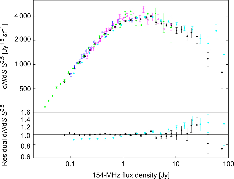
The GLEAM counts are generally in excellent agreement with the other counts. We note that GLEAM and TGSS are on different flux density scales, with TGSS on the scale of Scaife & Heald (Reference Scaife and Heald2012). There is, however, a flux-density-dependent offset between the GLEAM and TGSS counts. While the ratio of TGSS to GLEAM counts lies close to 1.0 at a few Jy, it decreases to ≈09. below ∼1 Jy. This is consistent with a ≈6% decrease in the mean ratio of TGSS to GLEAM flux densities below ∼1 Jy and may be due to missing low surface brightness emission in TGSS. The TGSS observations have a far less centrally concentrated uv coverage than the GLEAM observations. At 154 MHz, GLEAM has a resolution of ≈3 arcmin while TGSS has a resolution of 25 by 25/cos(δ − 19º) arcsec.

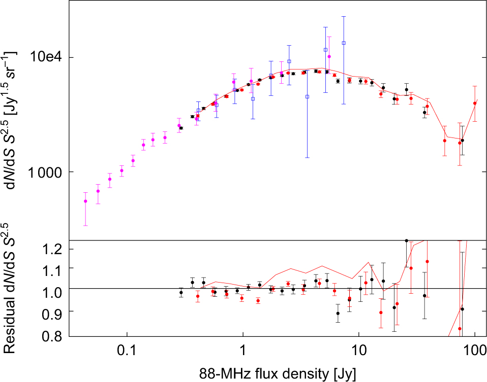
Source counts below 100 MHz are comparatively sparse. In Figure 7, we compare the 88-MHz GLEAM counts with the VLSSr counts at 74 MHz, placed on the Baars et al. (Reference Baars, Genzel, Pauliny-Toth and Witzel1977) flux density scale (Lane et al. Reference Lane, Cotton, van Velzen, Clarke, Kassim, Helmboldt, Lazio and Cohen2014); 62-MHz counts from LOFAR observations of the 3C295 and Boötes fields, covering 36 deg² (vanWeeren et al. Reference van Weeren2014); and 93.75-MHz counts from a 12-h pointed observation with the 21 Centimetre Array (CMA) of a 25 deg² region of sky coincident with the North Celestial Pole (Zheng et al. Reference Zheng, Wu, Johnston-Hollitt, Gu and Xu2016). The GLEAM counts, which cover the largest area of sky, show good agreement with the other counts extrapolated to 88 MHz with α = –0.8. Below ~1 Jy, the GLEAM counts lie very slightly (2–3%) above the VLSSr counts but this is sensitive to the spectral index used in the extrapolation. We note that VLSSr has a resolution of 75 arcsec as compared to the GLEAM resolution of ≈5 arcmin at 88 MHz.

Figure 7.

Top: Euclidean normalised differential counts in the frequency range 62–93.75 MHz, extrapolated to 88 MHz assuming α = −0.8. Black circles: this paper; red circles: Lane et al. (Reference Lane, Cotton, van Velzen, Clarke, Kassim, Helmboldt, Lazio and Cohen2014); blue squares: Zheng et al. (Reference Zheng, Wu, Johnston-Hollitt, Gu and Xu2016); purple circles: van Weeren et al. (Reference van Weeren2014). The red line displays the 74 MHz counts by Lane et al. (Reference Lane, Cotton, van Velzen, Clarke, Kassim, Helmboldt, Lazio and Cohen2014) scaled with α = −0.5. Bottom: the GLEAM and VLSSr counts are normalised with respect to a polynomial fit to the GLEAM counts to highlight differences.

5. Investigating changes in the source count shape with frequency

In this section, we analyse any change in the shape of the GLEAM counts with frequency and the dependence of the spectral index on flux density and frequency. We also show that the behaviour of the counts is broadly consistent with the typical spectra of sources across the MWA band.

The solid line in Figure 5 is a weighted least squares fifth-order polynomial fit to the GLEAM 154 MHz counts. We extrapolate the 200, 118, and 88 MHz GLEAM counts to 154 MHz assuming various spectral indices and divide the extrapolated counts by the 154-MHz source count fit calculated above, as shown in Figure 8.

Figure 8.

Top: the 200-MHz GLEAM counts are extrapolated to 154 MHz and divided by a polynomial fit to the 154-MHz GLEAM counts to highlight differences. The spectral index used in the extrapolation is –0.4 (dashed blue line), –0.6 (solid blue line), –0.8 (black circles), –1.0 (solid red line), and –1.2 (dashed red line). The 200-MHz counts are replaced by the 118- and 88-MHz counts in the central and bottom panels, respectively. At S _154MHZ > 0.5 Jy (dashed vertical line), α ≈ –0.8 provides a good match between the counts.

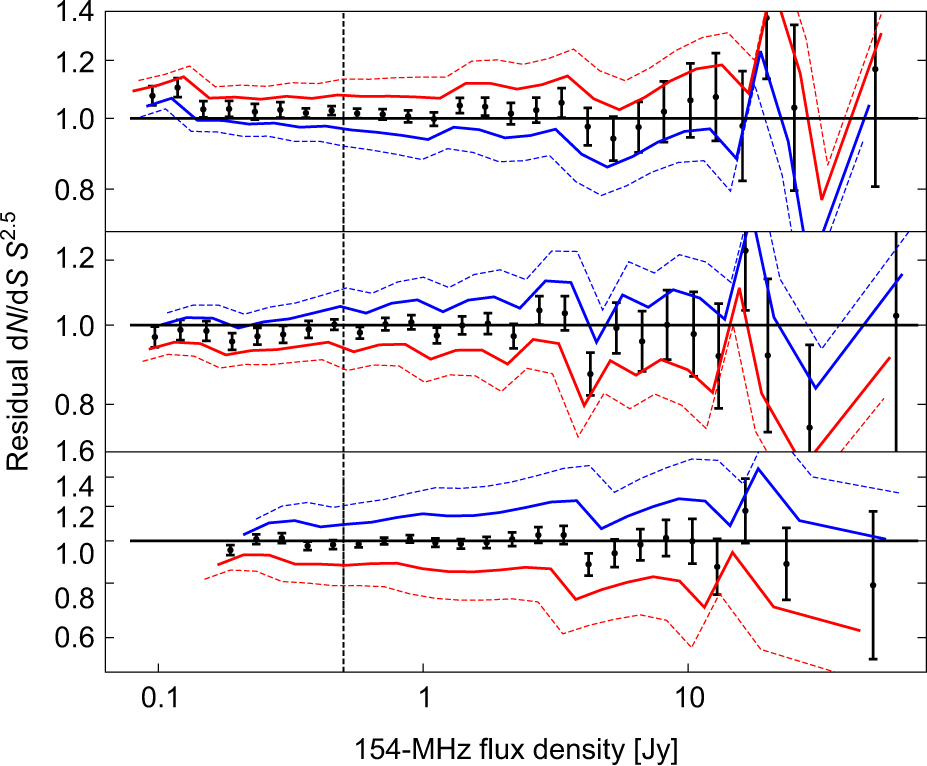
We find that, at S _154MHZ ≳ 0.5 Jy, there is no significant change in the shape of the counts at the four frequencies. We calculate the value of α which minimises the χ ² difference between the counts at each of the three pairs of frequencies. When computing χ ², we exclude the region of the 154-MHz source count fit below 0.5 Jy. For example, for the 154–200-MHz source count pair,

\begin{equation}{\chi ^2} = \Sigma _{i = 1}^N{w_i}{\left[ {{n_{i,200}} - y{n_{154}}\left( {{{{S_{i,200}}} \over x}} \right)} \right]^2},\end{equation}(5)

where

\begin{equation}{w_i} = \left\{ {\matrix{{{{\left[ {\sigma _{{n_{i,200}}}^2 + \sigma _{{n_{154}}({S_{i,200}}/x)}^2} \right]}^{ - 1}}} \hfill & {{\rm{if }}{{{S_{i,200}}} \over x} \gt 0.5 {\rm{Jy,}}} \hfill \cr 0 \hfill & {{\rm{otherwise}}{\rm{.}}} \hfill \cr } } \right.\end{equation}(6)

n_{i ,200} is the Euclidean normalised source count in the ith bin at 200 MHz, $ {\sigma _{{n_{i,200}}}} $ is the error on n_{i ,200}, $ {n_{154}}\left( {{{{S_{i,200}}} \over x}} \right) $ is the 154-MHz source count fit above evaluated at $ {{{S_{i,200}}} \over x} $, S_{i ,200} is the central flux density of the ith bin at 200 MHz, x = (200/154)^α, and y = x ^1.5. For the 154–200-, 154–118-, and 154–88-MHz source count pairs, χ ² is minimised with α = –0.75, –0.77, and –0.79, respectively. Thus there is no strong dependence of the spectral index on frequency.

At S _154MHZ < 0.5 Jy, it becomes hard to discriminate between different spectral indices given the steep slope of the counts. There is, however, tentative evidence that a flatter spectral index provides a better match between the 154–200- and 154–118-MHz source count pairs.

Hurley-Walker et al. (Reference Hurley-Walker2017) calculated the 76–227-MHz spectral indices of sources in the GLEAM catalogue using the 7.68-MHz sub-band flux densities. For the spectral index of a source to be quoted in the catalogue, the source must have a positive flux density in each of the 20 sub-bands (this is not always the case at low SNR) and the spectrum must be well fit by a power law. From the completeness maps presented in Hurley-Walker et al., in region B, the GLEAM catalogue is 90% complete at S _200MHz = 60 mJy. Of the 84 003 sources with S _200MHz > 60 mJy in region B, 75 905 (90.4%) have measured spectral indices in the GLEAM catalogue. Figure 9 shows the spectral index distribution for these sources. The distribution is roughly symmetric about the median value of –0.79 but there is a positive tail which extends to α ≈ 0.5.

Figure 9.

Spectral index distribution between 76 and 227 MHz for sources with S _200MHz > 60 mJy in region B of the GLEAM catalogue. The vertical dotted and dashed lines show the median and mean values of –0.79 and –0.76, respectively.

The top panel of Figure 10 shows the median spectral index, α _med, as a function of S _200MHz. Sources which are missing from the spectral index sample because they are not well fit by a power law are represented by the red histogram in the bottom panel. These sources include compact-steep spectrum (CSS) sources with a peak in their spectra across the MWA band, hypothesised to be the precursors to massive radio galaxies, and are studied in detail in Callingham et al. (Reference Callingham2017).

Figure 10.

Top: the black data points show the median 76–227-MHz spectral index as a function of flux density; the error bars are standard errors of the median. The red bars extend from the first to the third quartile. Bottom: percentage of sources which have no measured spectral indices in the GLEAM catalogue because they are not well fit by a power law (red) or because they have a negative flux density in at least one of the 7.68 MHz sub-bands (black).

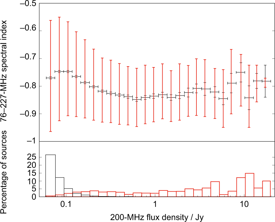
Above 0.5 Jy, we find that there is no significant change in the median spectral index, α _med, with flux density, whereas α _med flattens from ≈ –0.85 to ≈ –0.75 between 0.5 and 0.1 Jy. We caution that α _med is biased towards steep values below 0.1 Jy. Indeed, a substantial fraction of sources have no measured spectral indices in bins below 0.1 Jy because they do not have positive flux densities in all sub-bands; the negative flux densities mostly occur in lower frequency sub-bands due to the low SNR (see black histogram in bottom panel of Figure 10). This probably explains the steepening in α _med with decreasing flux density below 0.1 Jy.

Spectral flattening towards lower frequencies is expected for some sources due to absorption effects including synchrotron self-absorption and thermal absorption of a synchrotron power law component. Spectral ageing, which causes the spectrum to steepen towards higher frequencies, may introduce additional curvature in the source spectrum.

Given the weak dependence of the median redshift of radio galaxies on flux density (see e.g. Condon Reference Condon and Soifer1993), the flux density range 0.1 –0.5 Jy is expected to correspond to the least-luminous radio galaxies. By studying a number of complete samples of radio sources at frequencies close to 151 MHz with good coverage of the luminosity–redshift plane, Blundell, Rawlings, & Willott (Reference Blundell, Rawlings and Willott1999) found an anti-correlation between the rest-frame spectral index at low frequency and the source luminosity. This correlation is understood to arise through the steepening of the injection spectrum of particles by radiative losses in the enhanced magnetic fields of the hotspots of sources with more powerful jets. It is possible that the spectral flattening observed for GLEAM sources in this flux density range also results from this effect.

At S _{154 MHz} > 0.5 Jy, we find no evidence of any flattening in the average spectral index with decreasing frequency. van Weeren et al. (Reference van Weeren2014) measured source counts at 34, 46, and 62 MHz down to 136, 72, and 51 mJy, respectively, from LOFAR observations of the 3C295 and Boötes fields, covering a few tens of square degrees (their 62 MHz counts are displayed in Figure 7 of this paper). They found that (1) the 62-MHz counts are in good agreement with 153-MHz GMRT and 74-MHz VLA counts, scaling with α = –0.7; (2) the 34-MHz counts fall significantly below the extrapolated counts from 74 and 153 MHz with α = –0.7. Instead, α = –0.5 provides a better match to the 34-MHz counts.

6. Comparison with SKADS-Simulated Skies

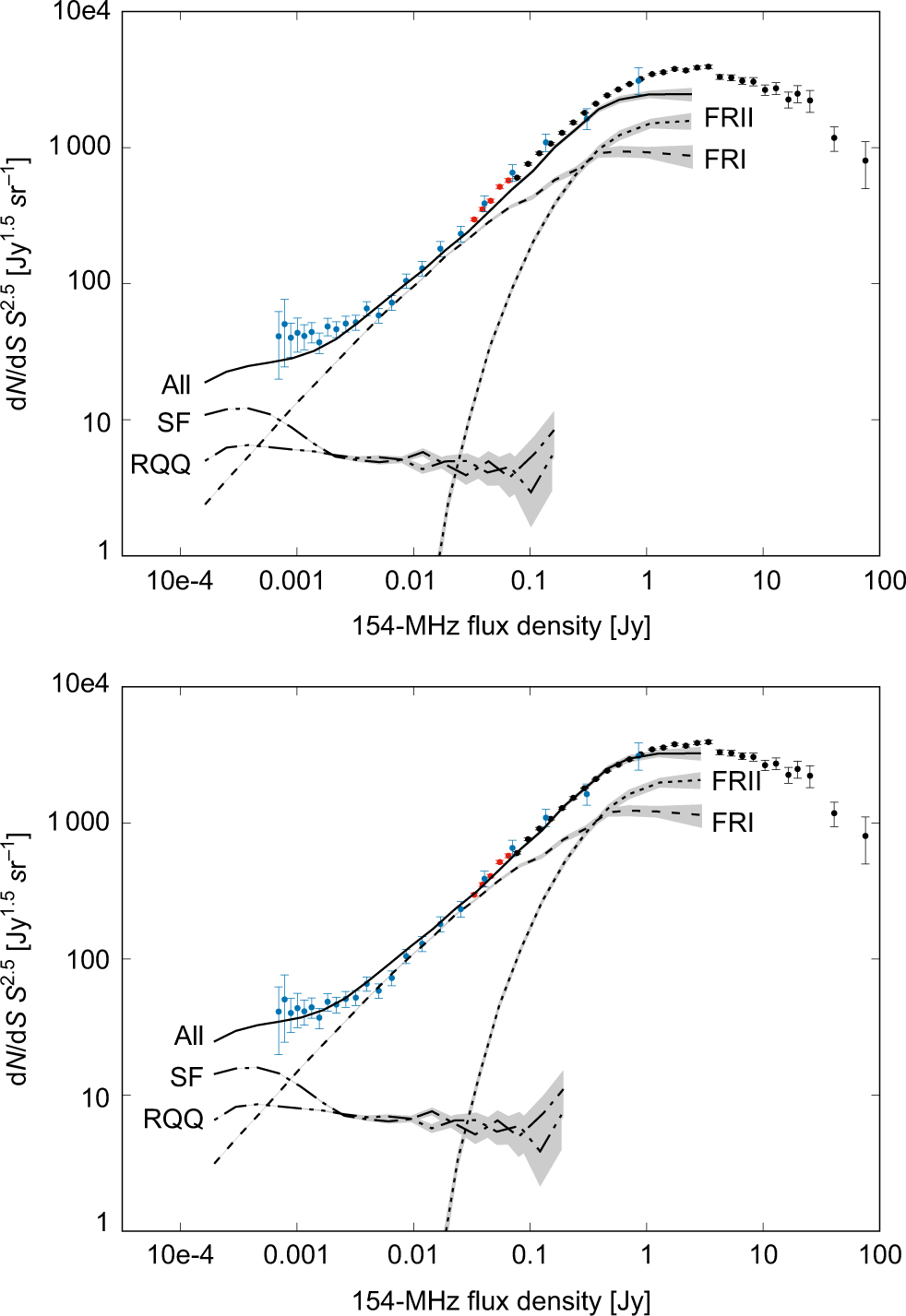
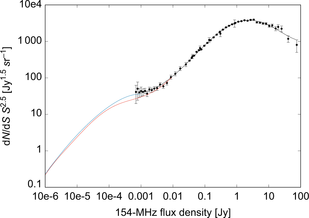
The SKADS model by Wilman et al. (Reference Wilman2008) gives radio flux densities at 151 MHz, 610 MHz, 1.4 GHz, 4.86 GHz, and 18 GHz, down to 10 nJy, in a sky area of 20 × 20 deg², and includes four distinct source types: FRI and FRII sources, radio-quiet AGN, and star-forming galaxies. We compare observed counts at 154 MHz covering over five orders of magnitude in flux density with the source count prediction from the simulated database. We use the 154-MHz GLEAM counts, the deeper MWA EoR counts in the flux density range 30–75 mJy, and 150-MHz LOFAR counts by Williams et al. (Reference Williams2016), extrapolated to 154 MHz with α = –0.8.

In the top panel of Figure 11, we see that the 151-MHz SKADS model lies within the scatter of the observations except at S ≳ 50 mJy, where it increasingly underpredicts the measured counts with flux density. The GLEAM counts provide a very stringent test above this flux density given their high precision. The model underpredicts the number of sources by ≈50% by ≈2 Jy. Since the model only covers 400 deg², the source population is too poorly sampled above this flux density to perform a precise comparison.

Figure 11.

Top: the data points show the counts from this paper (black), MWA counts from Franzen et al. (Reference Franzen2016) (red), and LOFAR counts from Williams et al. (Reference Williams2016) (blue) at 154 MHz. These are compared with the SKADS simulations by Wilman et al. (Reference Wilman2008), including contributions from FRI and FRII sources, star-forming galaxies, and radio-quiet AGN. The 151-MHz SKADS model count is extrapolated to 154 MHz assuming α = –0.8. The shaded area indicates the 1σ errors. Bottom: same as above except that the simulated flux densities in the model are multiplied by 1.2 to obtain a better fit to the data.

Mauch et al. (Reference Mauch2013) compared 325 MHz counts from a GMRT survey of the Herschel-ATLAS/GAMA fields with the SKADS model and found a similar result, albeit to a lower significance. They determined the 325 MHz simulated flux density by calculating the power law spectral index between 151 and 610 MHz. Their measured counts, which sample the flux density range 10–200 mJy, tend to lie slightly above the simulated counts above S _325MHz ≈ 0.5 mJy.

We find that the model is statistically in much better agreement with the data at high flux density after multiplying the simulated flux densities by 1.2, as shown in the bottom panel of Figure 11. The fit is also somewhat improved at the low flux density end sampled by LOFAR although the data points have larger error bars making it harder to assess the model’s accuracy.

Mauch et al. suggest that the simulated flux densities at low frequency could be too low as a result of excessive spectral curvature implemented in the model. However, it is difficult to see how this is possible: radio-loud AGN dominates the source population at S _{154 MHz} > 0.5 mJy in the model. The overwhelming majority of these sources have power law spectra between 154 MHz and 1.4 GHz, as the emission is lobe dominated.

At the bright end, the model is based on a compilation of source counts at 151 MHz by Willott et al. (Reference Willott2001). The GLEAM counts provide much tighter constraints. The model is also based on the 151-MHz luminosity function of high-luminosity radio galaxies by Willott et al. They chose to fit a Schechter luminosity function, whose exponential high-luminosity cut-off is likely too sharp to describe radio galaxies.

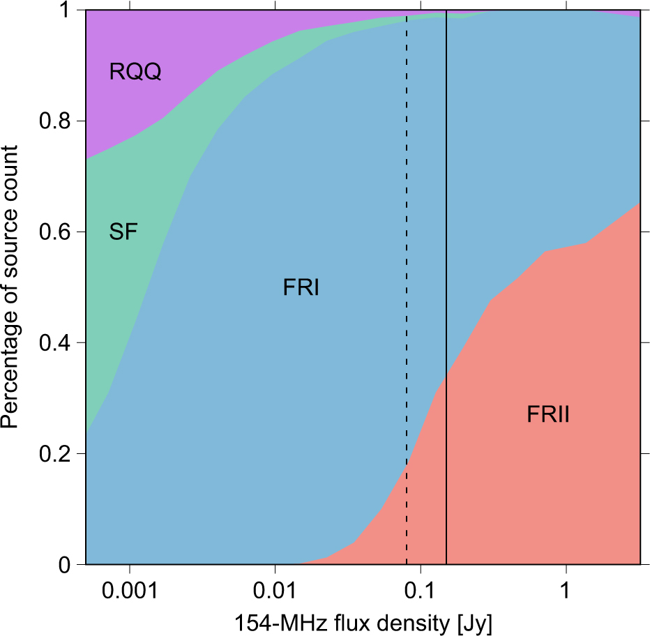
Figure 12 shows the fraction of each source type as a function of S _{154 MHz} as predicted by the SKADS model, after rescaling the simulated flux densities. According to the model, FRII sources are dominant above ~500 mJy, FRI sources in the flux density range ~1–500 mJy and star-forming galaxies below ~1 mJy.

Figure 12.

The population mix at 154 MHz as predicted by the SKADS model after multiplying the simulated flux densities by 1.2. For reference, the 154-MHz GLEAM counts are measured above 150 mJy (solid line) and 80 mJy (dashed line) in regions A and B, respectively.

7. Noise and confusion properties of GLEAM mosaics

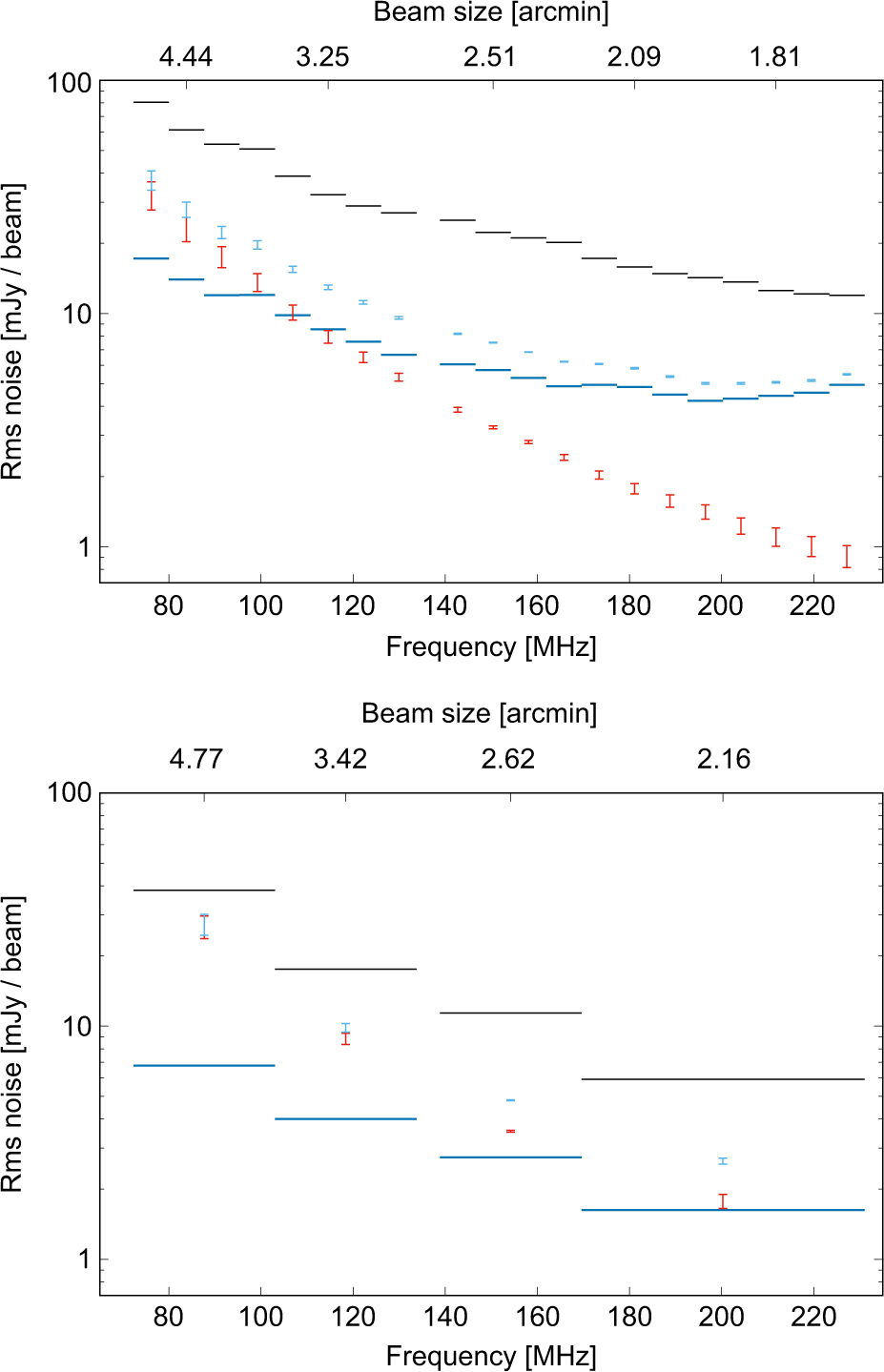
Figure 13 shows the mean rms noise, measured using bane, in the narrow- and wide-band mosaics in a circular region within 8.5º of the Chandra Deep Field-South (CDFS) at J2000 α = 03^h30^m, δ = –28º00 arcmin, hereafter referred to as region C; this region lies close to zenith (i.e. at δ = –26.7º) and 55º from the Galactic Plane.

We derive the expected thermal noise in this cold region of extragalactic sky. We then use our knowledge of the low-frequency source counts below the flux densities sampled by GLEAM to derive the theoretical noise limit, accounting for both the thermal noise and classical confusion, and compare it with the measured rms noise.

Figure 13.

Top: rms noise in the narrow-band mosaics in a region within 8.5º from CDFS (black horizontal bars), expected thermal noise sensitivity from Stokes V mosaics (blue horizontal bars), range of classical confusion noise estimates (red), and range of theoretical noise limits (turquoise points). The approximate beam size is shown on the top. Bottom: same as above in the wide-band mosaics.

7.1. Estimating the thermal noise

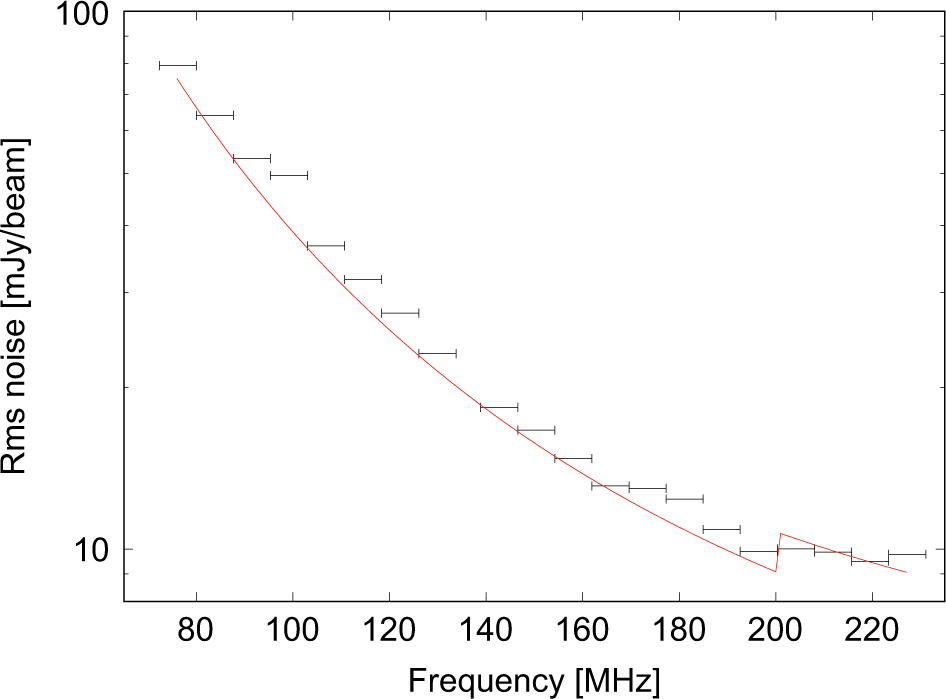
Since no circular polarisation is expected from extragalactic sources, Stokes V images should provide a good measure of the thermal noise. We download all narrow-band, uniformly weighted Stokes V snapshot images contributing to region C from the GLEAM Data Centre,Footnote ^boriginating from four different declination strips (–13º, –27º, –40º, and –55º). We verify that the rms noise in Stokes V images from the Dec –27º strip is in good agreement with the theoretical prediction.

The naturally weighted, point-source sensitivity of the MWA, in Jy/beam, is given by

\begin{equation}{\sigma _{\rm{t}}} = {{2{k_{\rm{B}}}T} \over {{A_{{\rm{eff}}}}{\varepsilon _{\rm{c}}}}}\sqrt {{1 \over {\tau B{n_{\rm{p}}}N(N - 1)}}} {\kern 1pt} ,\end{equation}(7)

where k _B is the Boltzmann constant, T the system temperature in K, A _eff the effective area of each antenna tile in m², N the number of antenna tiles, ɛ _c the correlator efficiency, τ the integration time in seconds, B the bandwidth in Hz, and n _p the number of polarisations (Tingay et al. Reference Tingay2013).

The system temperature is given by T = T _sky + T _rec, where T _sky is the sky temperature and T _rec the receiver temperature. Wayth et al. (Reference Wayth2015) present measurements of the average sky temperature for pointings at different declinations and local sidereal time at multiple GLEAM frequencies. From this information, we obtain T _sky ≈ 228 K (ν/150 MHz)^–2.53 at the location of the CDFS. Following Wayth et al. (Reference Wayth2015), we set T _rec = 50 K except at ν > 200 MHz, where we set T _rec = 80 K; laboratory measurements by Sutinjo, Ung, & Juswardy (Reference Sutinjo, Ung and Juswardy2018), indicate that T _rec = 80 K at ν > 200 MHz. We set B = 0.75 × 7.68 MHz given a 25% reduction in the bandwidth due to flagged edge channels. We set the remaining parameters as follows: A _eff = 21.5 m², N = 128, ϵ _c = 1.0, τ = 2 min, and n _p = 2. We also account for a 2.1-fold loss in sensitivity due to uniform weighting (Wayth et al. Reference Wayth2015). We find that the theoretical prediction agrees within 25% with the Stokes V noise measurements across the entire frequency range (see Figure 14).

Figure 14.

Horizontal bars: rms noise in uniformly weighted Stokes V snapshot images with a bandwidth of 7.68 MHz, centred within a few degrees from J2000 α = 03^h30^m, δ = 28º00 arcmin. Red curve: theoretical noise prediction using equation (7).

We combine all the Stokes V snapshot images to produce narrow- and wide-band Stokes V mosaics, following the procedure described in Hurley-Walker et al. (Reference Hurley-Walker2017) for Stokes I. We measure the mean rms noise in region C of each Stokes V mosaic. The blue horizontal bars in Figure 13 show our thermal noise estimates for the narrow- and wide-band mosaics.

7.2. Estimating the theoretical noise limit

Given a source count model and beam size, we use the method of probability of deflection (Scheuer Reference Scheuer1957) to derive the exact shape of the source P(D) distribution, P _c(D), that is the probability distribution of pixel values resulting from all sources present in the image. We then estimate the rms classical confusion noise, σ_c, from the core width of this distribution.

A detailed explanation of the equations used to derive the P _c(D) can be found in Vernstrom et al. (Reference Vernstrom2014). Briefly, we calculate the mean number of pixels per steradian with observed intensities between x and x + dx:

\begin{equation}R(x) {\rm{d}}x = \int_\Omega {{{\rm{d}}N} \over {{\rm{d}}S}}\left( {{x \over {B(\theta ,\phi )}}} \right)B{(\theta ,\phi )^{ - 1}} {\rm{d}}\Omega {\rm{d}}x,\end{equation}(8)

where dN/dS is the differential source count and x = SB (θ, ϕ) is the image response to a point source of flux density S at a point in the synthesised beam where the relative gain is B(θ, ϕ). The predicted P _c(D distribution is then computed from the Fourier Transform of R(x), such that

\begin{equation}P(D) = {{\cal F}^{ - 1}}[p(\omega )],\end{equation}(9)

where

\begin{equation}p(\omega ) = \exp \left[ {\int_0^\infty R(x) \exp (i\omega x) {\rm{d}}x - \int_0^\infty R(x) {\rm{d}}x} \right].\end{equation}(10)

The black curve in Figure 15 is a weighted least squares fifth-order polynomial fit to the 154-MHz GLEAM counts and the 150 MHz counts by Williams et al. (Reference Williams2016), extrapolated to 154 MHz with α = –0.8. The polynomial fit is given by

\begin{equation}\mathop {\log }\nolimits_{10} \left( {{S^{2.5}}{{{\rm{d}}N} \over {{\rm{d}}S}}} \right) = \sum\limits_{i = 0}^5 {a_i}{[\mathop {\log }\nolimits_{10} (S)]^i}{\rm{,}}\end{equation}(11)

where a ₀ = 3.52, a ₁ = 0.307, a ₂ = 0.388, a ₃ = –0.0404, a ₄ = 0.0351, and a ₅ = 0.00600. The fit is valid over the flux density range 1 mJy–75 Jy.

Figure 15.

The data points show the 154-MHz counts from this paper, Franzen et al. (Reference Franzen2016), and Williams et al. (Reference Williams2016). The black curve is a polynomial fit to these counts. The red curve shows the 151-MHz SKADS model count (Wilman et al. Reference Wilman2008), while the blue curve shows the 151-MHz SKADS model count, applying a flux density scaling factor of 1.2.

Since no 154-MHz source count data are available below ≈ 1 mJy, we use the 151-MHz SKADS model count after multiplying the simulated flux densities by 1.2 (see blue curve in Figure 15). We choose to apply this flux density scaling factor as the model is then in better agreement with the observed counts above 1 mJy, as shown in Section 6. At 1 mJy, there is minimal discontinuity between the rescaled SKADS model and the above polynomial fit to the observed counts. Our preferred model, source count model A, consists of our polynomial fit to the observed counts above 1 mJy and the rescaled SKADS model below 1 mJy.

Below a few milliJansky, the LOFAR counts have relatively large uncertainties and the 151-MHz SKADS model, displayed as the red curve in Figure 15, lies significantly below the LOFAR counts. There is minimal discontinuity between our polynomial fit to the observed counts and the SKADS model at 10 mJy. We therefore consider a second model, source count model B, consisting of the polynomial fit above 10 mJy and the SKADS model below 10 mJy.

In Section 5, we showed that a spectral index scaling of ≈ –0.8 provides a good match between the GLEAM counts at S _{154 MHz} > 0.5 Jy. It is not clear whether this continues to be the case at lower flux densities. We extrapolate the models to other frequencies with α = –0.6, –0.8, and –1.0 in order to gauge the effect of spectral indices flatter and steeper than –0.8 on σ_c.

In calculating P _c(D), we assume that the beam is a circular Gaussian with a full width at half-maximum (FWHM) $ \theta {\kern 1pt} = {\kern 1pt} \sqrt {{a_{{\rm{psf,mean}}}}{b_{{\rm{psf,mean}}}}} $, where a _psf,mean and b _psf,mean are the mean values of a _psf and b _psf in region C of the PSF map, respectively. This accounts for the increase in area of the PSF, resulting from ionospheric smearing.

The black curve in Figure 16 shows the P _c(D) distribution that we derive in the wide-band image at 139–170 MHz using source count model A, where θ = 2.6 arcmin. The width of the distribution is measured by dividing the interquartile range by 1.349, i.e. the rms for a Gaussian distribution, obtaining σ_c = 3.6 mJy/beam.

Figure 16.

Source P(D) distribution (black curve), thermal noise distribution (red curve), and source P(D) distribution convolved with thermal noise distribution (blue curve) in region C of the 139–170-MHz GLEAM mosaic. The source P(D) distribution was derived using source count model A.

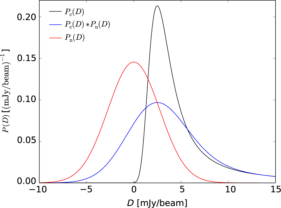
To account for the thermal noise, σ_t, P _c(D) must be convolved with the thermal noise distribution, P _n(D), represented as a Gaussian with rms σ_t. The convolution of P _c(D) with P _n(D) can be expressed as

\begin{equation}{P_{\rm{c}}}(D)*{P_{\rm{n}}}(D) = {{\cal F}^{ - 1}}\left[ {p(\omega ) \exp \left( {{{ - \sigma _{\rm{t}}^2{\omega ^2}} \over 2}} \right)} \right].\end{equation}(12)

Our thermal noise estimate in region C of the 139–170 MHz mosaic is 2.7 mJy/beam. The red curve in Figure 16 is a Gaussian centred on zero with a standard deviation of 2.7 mJy/beam, representing P _n(D), while the blue curve is the convolution of P _c(D) with P _n(D). The blue curve has a core width of 4.8 mJy/beam, and we take this to be the theoretical noise limit, σ_lim.

We follow this procedure to derive σ_c and σ_lim for the narrow- and wide-band mosaics at all frequencies. We derive σ_c and σ_lim using both 154 MHz source count models and α = –0.6, –0.8, and –1.0 to extrapolate the models to other frequencies. The range of σ_c and σ_lim values is displayed in Figure 13. We find that, at 154 MHz, σ_c changes by no more than 3% depending on the source count model adopted. Varying the spectral index has a greater effect on σ_c at the upper and lower ends of the GLEAM frequency range.

8. Origin of excess background noise in GLEAM images

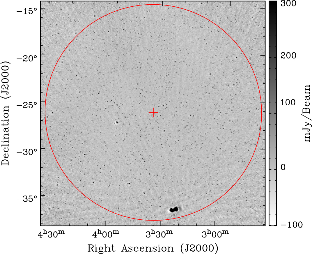
Possible causes of the excess background noise in GLEAM images include sidelobe confusion, calibration errors, background emission from the Galactic Plane, and extended sources not included in the source count model used to derive σ_c. We analyse the noise contribution in a GLEAM snapshot image at 139–170 MHz with a beam size of 2.4 arcmin, lying close to the CDFS; the image is displayed in Figure 17. We then predict the visibilities for the measurement set using a realistic distribution of point sources and image the simulated uv data using exactly the same parameters in wsclean as those used to image the real data. By comparing the P(D) distributions in the real and simulated images, we show that the excess background noise is primarily caused by confusion from sidelobes of the ideal synthesised beam. Finally, we attempt to approach the theoretical noise limit using an improved deconvolution method.

Figure 17.

GLEAM snapshot image at 139–170 MHz after primary beam correction. The image is centred close to the CDFS and Fornax A is visible in the south of the image. The red circle shows the half-power contour of the primary beam.

8.1. Noise properties of a real GLEAM snapshot image at 139–170 MHz

We use the method described in Section 7.2 to calculate P _c(D) * P _n(D) within the half-power contour of the primary beam. We derive P _c(D) given the beam size of 2.4 arcmin and assuming source count model A.

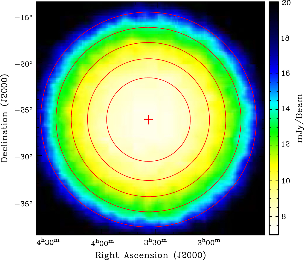
Figure 18 shows the rms noise map of the Stokes V image. The thermal noise in the centre of the field is 8 mJy/beam but varies by a factor of two across the field given the primary beam response. It follows that the thermal noise distribution cannot be well approximated as a Gaussian. To address this problem, we divide the region into five concentric annuli such that the thermal noise varies by no more than 20% in each annulus. The thermal noise in each annulus, σ_t,i is taken as the mean rms noise in each annulus of the Stokes V image. P _c(D) * P _n(D) is then taken as

\begin{equation}{{\sum\limits_{i = 1}^5 {A_i} {P_{\rm{c}}}(D)*{P_{{\rm{n}},i}}(D)} \over {\sum\limits_{i = 1}^5 {A_i}}},\end{equation}(13)

where P _{n, i} (D) is a Gaussian of width σ_{t, i} representing the thermal noise distribution in the ith annulus and A_i is the area of the ith annulus.

Figure 18.

Rms noise map of the Stokes V snapshot image, representative of the thermal noise. The red circles show the concentric annuli into which the image was divided to calculate P _c(D) * P _n(D).

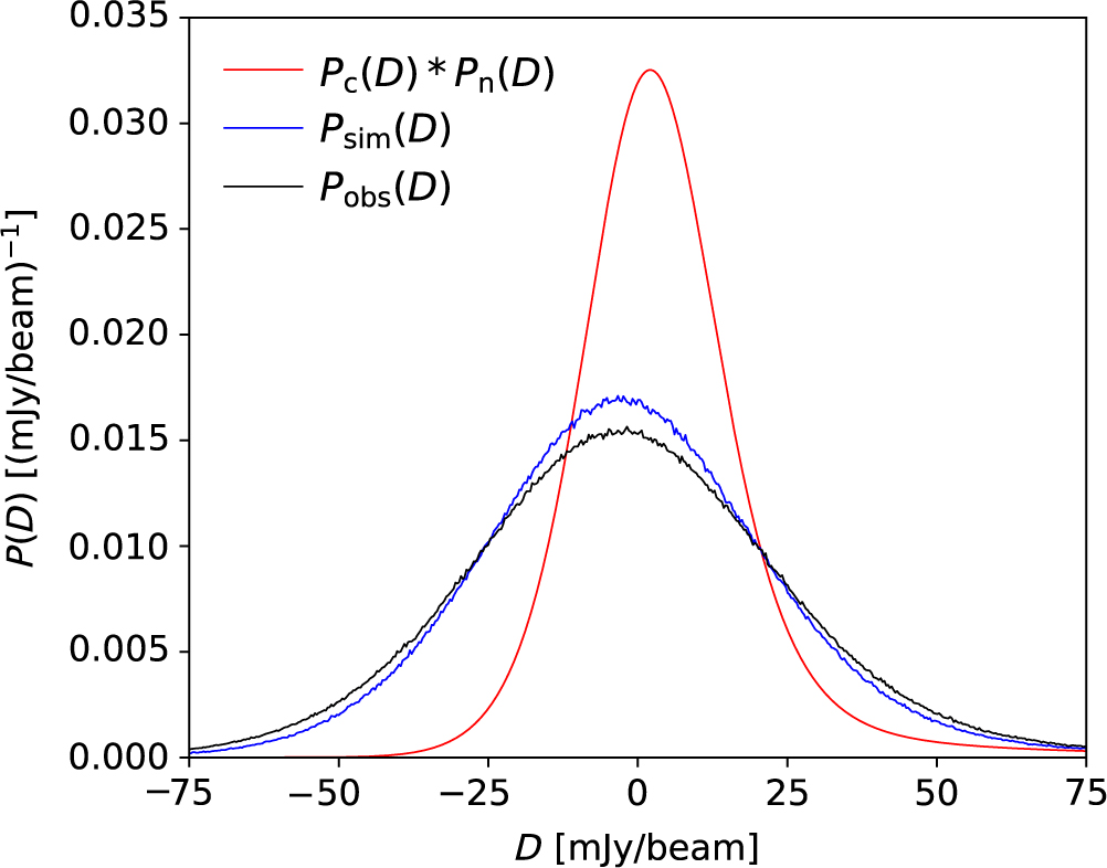
The observed P(D) distribution within the half-power contour of the primary beam, P _obs(D), is compared with P _c(D) * P _n(D) in Figure 19. The theoretical noise limit obtained from the core width of P _c(D) * P _n(D) is 12.7 mJy/beam. In comparison, the core width of P _obs(D), σ_obs = 26.3 mJy/beam.

Figure 19.

The P _obs(D) distribution is shown in black, P _c(D) * P _n(D) distribution in red, and P _sim(D) distribution in blue.

8.3. Improving the deconvolution

The GLEAM snapshot referred to at the beginning of Section 8 was imaged using wsclean v1.10. The pixel size was set to 32.7 × 32.7 arcsec² and the image size to 4000 × 4000 pixels, such that the image encompasses the ≈10% level of the primary beam. The snapshot was imaged down to the first negative CLEAN component. The rms noise of this initial image, σ = 50 mJy/beam, was measured and the snapshot was re-imaged down to a CLEAN threshold of 3σ (150 mJy/beam). In practice, this CLEANing strategy generally leaves significant residual emission undeconvolved.

We re-image the snapshot using wsclean v2.5, which is more efficient for large images thanks to the implementation of the Clark CLEAN algorithm (Clark Reference Clark1980). In minor CLEAN cycles, CLEAN components are subtracted from the image using only the central portion of the PSF and only the largest residuals are searched. This is sufficient to find the CLEAN components providing that the synthesised beam is well behaved; the accuracy of the subtraction is improved during major CLEAN cycles where the FT of the CLEAN components is subtracted from the residual visibility data.

Using wsclean v2.5, we CLEAN the entire image to 3σ, construct a mask from the identified CLEAN components, and continue CLEANing with the mask to 1σ. This is conducted in an automated fashion using the ‘auto-mask’ and ‘auto-threshold’ parameters. It is not necessary to provide wsclean with an estimate of σ as the algorithm automatically calculates the standard deviation of the residual image before the start of every major CLEAN cycle, which it then uses to set the CLEAN threshold. This is desirable since, in practice, the noise can drop considerably after the first few major CLEAN cycles as the image quality improves. The use of a mask permits CLEANing down to the noise level.

The total number of CLEAN iterations using wsclean v2.5 is ≈ 190000 while it is only ≈ 25000 using wsclean v1.10. Despite the much larger number of CLEAN iterations, the processing time for wsclean v2.5 is ≈ 4 times shorter. The P(D) distributions obtained using the two versions of wsclean are compared with the theoretical noise limit in Figure 20. There is a ≈29% reduction in σ_obs using wsclean v2.5.

Figure 20.

Observed P(D) distributions obtained using different versions of wsclean and image sizes. The theoretical noise limit is shown in red.

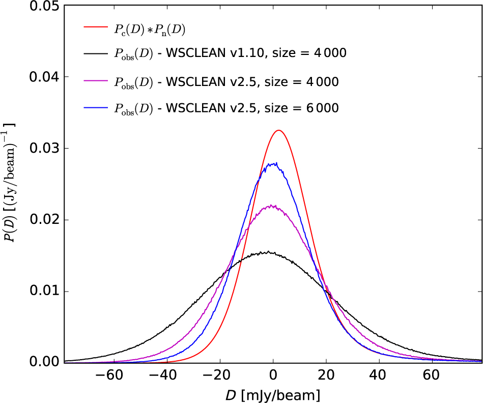
We investigate whether the noise can be reduced further by increasing the size of the region being CLEANed. We re-run wsclean v2.5 increasing the image size from 4000 × 4000 to 6000 × 6000 pixels. The imaged field-of-view now encompasses the first null of the primary beam. The resulting P(D) distribution is displayed in Figure 20. There is a further ≈21% reduction in σ_obs, which is now only ≈15% above σ_lim.

The results of this analysis are summarised in Table 4. We conclude that both the limited CLEANing depth and far-field sources that have not been deconvolved contribute significantly to the sidelobe confusion in GLEAM. The Clark optimisation is highly effective for large MWA images, permitting deeper CLEANing. We recommend adopting this technique in the future to ensure full exploitation of MWA survey images with the auto-masking and deeper thresholding.

Table 4.

Key parameters recorded for three different runs of wsclean on a 154-MHz snapshot image (see text for details). The theoretical noise limit is 12.7 mJy/beam.

9. Prospects for MWA phase 2

Since the GLEAM survey observations were carried out, the MWA has been upgraded with the addition of a further 128 tiles, 56 of which lie on baselines up to ≈6 km, roughly improving the array resolution by a factor of two (Wayth et al. Reference Wayth2018). The correlator capacity was not increased in Phase 2 of the MWA, so it is still only possible to correlate 128 tiles. In this section, we give an overview of how we expect σ_c and the rms sidelobe confusion noise, σ_s, to change for MWA Phase 2 observations.

We use the miriad (Sault, Teuben, & Wright Reference Sault, Teuben, Wright, Shaw, Payne and Hayes1995) task uvgen to simulate an image of the MWA Phase 2 PSF for a 2-min snapshot with a central frequency of 154 MHz and a bandwidth of 30.72 MHz, using a uniform weighting scheme. We fit a Gaussian to the main lobe of the synthesised beam; the geometric average of the major and minor axes of the fitted Gaussian is 1.15 arcmin. We use the method described in Section 7.2 to derive σ_c as a function of frequency for MWA Phase 2, setting the beam size θ _Phase2 = 1.15 arcmin (ν/154 MHz)^–1. We find that σ_{c,Phase 1}/σ_c,Phase2 varies from ≈5 at the high end of the band to ≈7 at the low end of the band, as shown in the top panel of Figure 21. The top panel of Figure 21 also includes estimates of σ_c for larger, hypothetical arrays with maximum baselines of 9, 12, and 18 km, where we set the beam size to $ {2 \over 3}{\theta _{{\rm{Phase 2}}}}, \ {1 \over 2}{\theta _{{\rm{Phase 2}}}} $, and $ {1 \over 3}{\theta _{{\rm{Phase 2}}}} $, respectively.

Figure 21.

Top: classical confusion noise as a function of frequency for MWA Phase 1 (black), MWA Phase 2 (red), and larger, hypothetical arrays with maximum baselines of 9 km (blue), 12 km (purple), and 18 km (turquoise). Bottom: classical confusion noise at 154 MHz as a function of beam size. The diagonal lines show power law fits to the data points in three different θ ranges. Dashed lines indicate the beam sizes at 154 MHz for the different arrays.

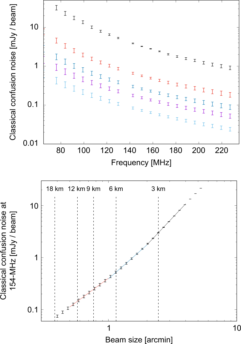
The classical confusion noise at 154 MHz as a function of beam size is also displayed in the bottom panel of Figure 21. We fit the function σ_c = aθ^b in three different θ ranges and find that b drops with decreasing θ, with b = 2.61 for θ = 2.0–4.0 arcmin, b = 2.18 for θ = 1.0–2.0 arcmin, and b = 1.83 for θ = 0.5–1.0 arcmin. Condon (Reference Condon1974) showed that for a power law differential source count n(S) = kS ^–γ, $ {\sigma _{\rm{c}}} \propto {\theta ^{{2 \over {\gamma - 1}}}} $. The flattening of the 154-MHz Euclidean normalised differential counts below ≈10 mJy (corresponding to an increase in γ) can therefore explain the drop in b with decreasing θ.

Bowman, Morales, & Hewitt (Reference Bowman, Morales and Hewitt2009) derive an expression for the variance in the intensity of a dirty sky map assuming that the primary and synthesised beams are described by top-hat functions, such that the response is defined to be one within a region of diameter Θ_P in the case of the primary beam and within a region of diameter Θ_B in the case of the synthesised beam. Outside this region, the response is taken to be zero for the primary beam and a constant value of B _rms ≪ 1 for the synthesised beam, representing the standard deviation of the synthesised beam sidelobes. With these simplifications,

\begin{equation}{\sigma _{\rm{s}}} \approx {\sigma _{\rm{c}}}{B_{{\rm{rms}}}}\sqrt {{{{\Omega _{\rm{P}}}} \over {{\Omega _{\rm{B}}}}}} {\kern 1pt} ,\end{equation}(14)

where $ {\Omega _{\rm{B}}} \approx \Theta _{\rm{B}}^2 $ is the solid angle of the synthesised beam and $ {\Omega _{\rm{P}}} \approx \Theta _{\rm{P}}^2 $ is the solid angle of the primary beam.

For the MWA, B _rms varies strongly with distance, d, from the beam centre. We measure B _rms in MWA Phase 1 and 2 PSF images as a function of d (see Figure 22). Since B _rms,Phase1 ≳ 2 B _{rms,Phase 2}, Ω_P,Phase1 = Ω_{P,Phase 2}, and Ω_B,Phase1 ≈ 4 Ω_{B,Phase 2},

\begin{equation}{{{\sigma _{{\rm{s, Phase 1}}}}} \over {{\sigma _{{\rm{s, Phase 2}}}}}} \mathbin{\lower.3ex\hbox{$\buildrel \gt \over{\smash{\scriptstyle\approx}\vphantom{_2}}$}} {{{\sigma _{{\rm{c, Phase 1}}}}} \over {{\sigma _{{\rm{c, Phase 2}}}}}}{\kern 1pt} .\end{equation}(15)

Figure 22.

Comparison of the MWA phase 1 (black) and 2 (red) synthesised beams for a 2-min snapshot with a central frequency of 154 MHz and bandwidth of 30.72 MHz, using a uniform weighting scheme. The standard deviation of the pixel values in the synthesised beam is plotted as a function of distance from the pointing centre. The standard deviation is calculated in a thin annulus at the given radius.

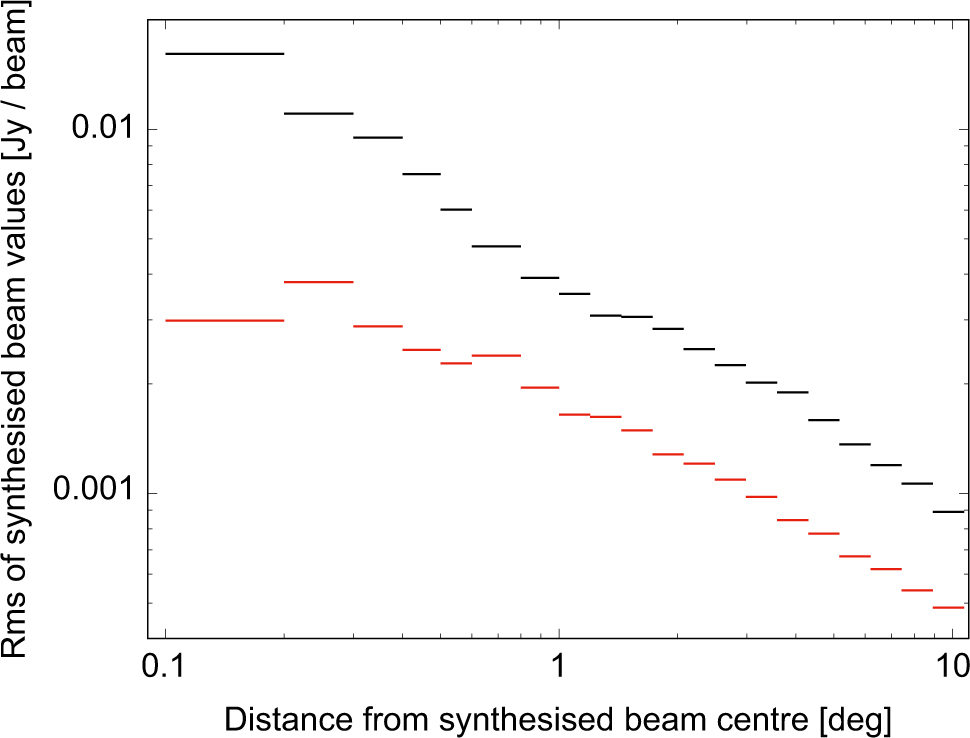
We therefore expect that σ_{s,Phase 1}/σ_s,Phase2 ≳ 5 across the MWA frequency range, assuming that the MWA Phase 1 and 2 images are CLEANed to the same flux density threshold. We must also consider that MWA Phase 2 images will take longer to image because of the increased resolution. The calibration of MWA Phase 2 data will be more challenging and, depending on the ionospheric conditions, direction-dependent calibration techniques will probably be required to reach the theoretical noise limit (see e.g. Offringa et al. Reference Offringa2016; Rioja, Dodson, & Franzen Reference Rioja, Dodson and Franzen2018).

10. Summary and future work

GLEAM is a contiguous 72–231 MHz survey of the entire sky south of declination +30º and has the widest fractional bandwidth and highest surface brightness sensitivity among low radio frequency surveys. We have determined the GLEAM source counts at 200, 154, 118, and 88 MHz to a flux density limit of 50, 80, 120, and 290 mJy, respectively, to high precision. The 200-MHz counts are based on the GLEAM extragalactic catalogue by Hurley-Walker et al. (Reference Hurley-Walker2017). From the three lowest 30.72-MHz sub-band images of GLEAM, we have constructed additional, statistically complete source samples at 154, 118, and 88 MHz to measure the counts at these frequencies.

The counts at 154 and 88 MHz are overall in good agreement with other counts in the literature at a similar frequency. The 151-MHz SKADS model significantly underpredicts the 154-MHz GLEAM counts at S ≳ 50 mJy. The cause of the discrepancy is unclear. The model is based on the 151-MHz luminosity function of high-luminosity radio galaxies by Willott et al. (Reference Willott2001), which in turn was determined using measurements of the local radio luminosity function (LRLF) for AGN. Since no measurements of the LRLF for AGN were available at 151 MHz, Willott et al. used the LRLF for AGN at 1.4 GHz by Cotton Condon (Reference Cotton and Condon1998) and made a simple shift in radio power assuming α = –0.8. They also chose to fit a Schechter luminosity function, whose exponential high-luminosity cut-off is likely too sharp to describe radio galaxies. We find that the model is statistically in much better agreement with the data after multiplying the simulated flux densities by 1.2.

At S _{154 MHz} > 0.5 Jy, there is no discernible change in the shape of the counts at the four frequencies: a spectral index scaling of ≈ –0.8 provides a good match between the counts. The spectra of individual sources show, on average, a slight but significant flattening of $ \delta \alpha _{76}^{227} \approx 0.1 $ between 0.5 and 0.1 Jy.

We may have expected to see a change in the source count shape with frequency due to spectral curvature of generations of sources at different redshifts. The fact that GLEAM is overwhelmingly dominated by sources with steep power law spectra indicates that there is no simple way of tracing ageing or evolution of the bright source population from this set of frequencies.

The low-frequency emission from star-forming galaxies remains largely unstudied. Detailed measurements of their spectra are important for understanding the physical processes which contribute to the radio emission from star formation. They can also be used to construct more accurate low-frequency source counts, which will be invaluable for planning deep low-frequency surveys with future facilities. Galvin et al. (Reference Galvin2018) measured the radio spectra of 19 luminous infrared galaxies (LIRGs) at 0.067 < z < 0.227 using GLEAM and Australia Telescope Compact Array (ATCA) follow-up observations at 2.1–45 GHz. They found that many of the sources exhibit low-frequency turnovers in their spectra which can be attributed, in large part, to free-free absorption. Deep LOFAR observations in small-area fields are also probing the low-frequency behaviour of star-forming galaxies. The LoTSS is expected to detect hundreds of thousands of star-forming galaxies, primarily at lower redshifts but extending out to z ≥ 1.

Although GLEAM is overwhelmingly dominated by radio-loud AGN, the SKADS model predicts that GLEAM contains 375 ± 80 local (z < 0.1) star-forming galaxies with S _200MHz > 50 mJy in region B, covering ≈6500 deg². In a future paper, we will cross-match the GLEAM catalogue with nearby optical samples to determine the LRLF for both AGN and star-forming galaxies at 154 MHz. We will correlate the local radio sample with higher frequency surveys including NVSS and SUMSS to characterise the typical spectra of these two populations. We also plan to investigate changes in the spectral behaviour of AGN with respect to radio morphology and luminosity.

Using deep 150-MHz LOFAR counts by Williams et al. (Reference Williams2016) and the SKADS model, we have conducted a P(D) analysis to derive the classical confusion noise in GLEAM images. While the images are limited by classical confusion below ≈100 MHz, the rms noise is a factor of ≈2 higher than the theoretical noise limit, accounting for both the thermal noise and classical confusion, at higher frequencies. By analysing a synthetic snapshot image containing a realistic distribution of point sources, we have demonstrated that the excess background noise is primarily due to confusion from sidelobes of the ideal synthesised beam. We have shown that we can approach the theoretical noise limit using the Clark CLEAN algorithm implemented in wsclean, along with deeper deconvolution and larger image size to encompass the first null of the primary beam.

For the MWA Phase 2 array with the angular resolution improved by a factor of two, we anticipate that both the classical and sidelobe confusion noise will drop by a factor of ≈5 at the high end of the band. Deep pointed observations of the Galaxy and Mass Assembly (GAMA; Driver et al. Reference Driver2009) 23 field, centred at Dec –32.5º, have been made with MWA Phase 2 (N. Seymour et al., in preparation) at 72–231 MHz with the goal of producing a radio luminosity function and investigating its dependence on MWA in-band spectral index. This work will demonstrate the ‘deep’ imaging quality which MWA Phase 2 can provide and will include an investigation of the factors which affect the noise.