


1 Introduction
Overestimation of voter turnout has been a persistent challenge for election surveys. Since the late 1940s, turnout estimates from the American National Election Study (ANES) have consistently exceeded official reports, often by more than 15 percentage points in recent presidential elections (Brehm Reference Brehm2009; Burden Reference Burden2000; Dahlgaard et al. Reference Dahlgaard, Hansen, Hansen and Bhatti2019; Enamorado and Imai Reference Enamorado and Imai2019; Jackman and Spahn Reference Jackman and Spahn2019). A key source of bias is the presence of nonignorable nonresponse bias: those who do not vote are less likely to respond to the election survey (Berent, Krosnick, and Lupia Reference Berent, Krosnick and Lupia2011; Sciarini and Goldberg Reference Sciarini and Goldberg2017). In this situation, the missingness is typically related to the unobserved outcome itself, referred to as nonignorable or missingness not at random (MNAR; Little and Rubin Reference Little and Rubin2019), making valid adjustment substantially more challenging than under the missingness at random (MAR) assumption, where the missingness is independent of the missing outcome conditional on fully observed covariates.
Recent work has developed parametric and auxiliary variable-based approaches for MNAR adjustment (Heckman Reference Heckman1979; Liu et al. Reference Liu, Miao, Sun, Robins and Tchetgen2020; Miao and Tchetgen Reference Miao and Tchetgen2016; Miao, Ding, and Geng Reference Miao, Ding and Geng2016; Sun et al. Reference Sun, Liu, Miao, Wirth, Robins and Tchetgen2018). Notably, Bailey (Reference Bailey2024, Reference Bailey2025) proposed a randomized response instrument (RRI) framework by using randomized treatments as response instruments to adjust for nonresponse bias, which is an important step in advancing political survey research toward MNAR-based analysis. Alternatively, a promising direction is the use of callback data—records about the data collection process. In political surveys, callback data are particularly valuable, as they record the effort needed to obtain responses and are widely available (Biemer, Chen, and Wang Reference Biemer, Chen and Wang2013; Couper Reference Couper1998; Olson Reference Olson2013). With callback data, the continuum of resistance (COR) model approximates nonrespondents by the most reluctant respondents (Clarsen et al. Reference Clarsen, Skogen, Nilsen and Aarø2021; Lin and Schaeffer Reference Lin and Schaeffer1995), although, in certain situations, nonrespondents are still quite different from the hardest-to-reach respondents, limiting the model’s ability to fully correct nonresponse bias in certain contexts.
This article introduces a stableness of resistance (SOR) model for leveraging callback data to adjust for nonignorable nonresponse and applies it to the ANES Non-Response Follow-Up (NRFU) survey concerning the 2020 U.S. presidential election to estimate the voter turnout. It offers a promising complement to the RRI framework of Bailey (Reference Bailey2025). The SOR model assumes that the impact of the missing outcome on the resistance or willingness to respond remains the same across the first two call attempts. Similar ideas have been applied by Alho (Reference Alho1990), Guan, Leung, and Qin (Reference Guan, Leung and Qin2018), Kim and Im (Reference Kim and Im2014), Peress (Reference Peress2010), and Qin and Follmann (Reference Qin and Follmann2014) with a fully parametric propensity score model. Building on a previous framework (Miao et al. Reference Miao, Li, Zhang and Sun2025), this article adopts a semiparametric approach that only requires partially parametric specification of the joint distribution, and extends the framework of Miao et al. (Reference Miao, Li, Zhang and Sun2025) to accommodate the joint missingness of both the outcome and covariates, using census data to recover the covariates distribution. We develop semiparametric estimators, including a doubly robust one that yields consistent estimates when either the second-call response propensity model or the outcome model is correctly specified, provided correct specification of the first-call response propensity model and an odds ratio model about the outcome–missingness relationship.
Our analysis produces turnout estimates closely aligned with official reports, provides strong evidence of nonignorable nonresponse in the NRFU survey and reveals systematic heterogeneity in survey participation and voting behavior. For example, women and senior people are more likely to respond, better-educated and senior people are more likely to vote, while Hispanics exhibit lower likelihoods of both responding and voting. Besides, the association between design covariates and response may be heterogeneous across different demographic groups, for instance, visible cash incentives tend to increase response rates more among men than among women. These findings highlight both the methodological potential of callback data and the practical implications for designing future political surveys.
2 The ANES 2020 NRFU study
The ANES 2020 NRFU study is a follow-up to the ANES 2020 Time Series Study, designed to collect data to analyze nonresponse bias, providing a valuable case study to explore self-reported turnout. The study was conducted by mail with 8,000 addresses from the ANES 2020 Time Series Study, constituting a weighted sample from the original ANES population. It began on January 28, 2021, with an advance postcard randomly sent as part of a factorial design. The study contains a two-stage callback design: The first class invitation was mailed on February 1, followed by the second class invitation sent to nonrespondents in the first class with replacement questionnaire on March 2 and March 30. This survey procedure provides us with high-quality callback data for nonresponse adjustment. Besides, reminder postcards were sent on February 16 and April 5.
The NRFU study also embedded a factorial design for several methodological experiments to investigate the effects of mail-based design features on the response rate, concerning the study title, advance postcard, questionnaire length and content and visible cash incentives. These methodological experiments are independently randomized.
After two callback stages, the NRFU survey closed on June 1, 2021, with 3,779 completed questionnaires. The response rate is 48.3% after excluding 168 undeliverable, deceased and removed cases from the total samples. According to McDonald (Reference McDonald2024), the official turnout in voting-age population (VAP) and voting-eligible population (VEP) in the 2020 presidential election is 62.0% and 66.4%, respectively. Since the ANES sampling framework excludes noncitizens, the VEP rate can be viewed as an approximation to the true turnout of ANES population. However, the weighted voter turnout based on the respondents in the NRFU study is over 85%, which is much higher than the VEP or VAP turnout, indicating a severe nonresponse bias.
3 Methodology
3.1 Model assumptions and identification
In this section, we illustrate how to use callback data and external census data to identify the true turnout and adjust for nonresponse bias in the NRFU study, where both demographic covariates and outcomes are subject to missingness due to nonresponse. Intuitively, callback data reflect the reluctance of units to respond and differences in turnout across callback stages suggest an association between voting and response propensity, indicating nonignorable nonresponse. In the NRFU survey, voter turnout declines from 87.9% among first-call respondents to 81.9% among second-call respondents, and falls to 42.4% among nonrespondents (based on VEP). This declining trend provides empirical evidence that harder-to-reach individuals are less likely to vote, motivating our modeling strategy to adjust for such nonignorable nonresponse using callback data.
Data structure of a survey with callbacks

Note: NA stands for missing values.
We now formalize this idea. Let Y denote the voting behavior, with $Y=1$
indicating that an individual voted and
$Y=1$
indicating that an individual voted and $Y=0$
otherwise. We are interested in the outcome mean
$Y=0$
otherwise. We are interested in the outcome mean $E(Y)$
, that is, the voter turnout in the ANES population. Let X denote a vector of covariates collected in the survey, possibly including components
$E(Y)$
, that is, the voter turnout in the ANES population. Let X denote a vector of covariates collected in the survey, possibly including components $X_1$
(e.g., age and gender) that are missing together with Y and also components
$X_1$
(e.g., age and gender) that are missing together with Y and also components $X_2$
that are fully observed. Note that
$X_2$
that are fully observed. Note that $X_2$
could be an empty set. In the NRFU study,
$X_2$
could be an empty set. In the NRFU study, $(X_1,Y)$
are missing for nonrespondents, and
$(X_1,Y)$
are missing for nonrespondents, and $X_2$
is a vector related to the factorial design experiments, for example, questionnaire version and whether the prepaid cash incentives are visible. The experimental design is randomized, that is,
$X_2$
is a vector related to the factorial design experiments, for example, questionnaire version and whether the prepaid cash incentives are visible. The experimental design is randomized, that is, $X_2$
is independent of
$X_2$
is independent of $X_1$
. To simplify the notation, we no longer isolate demographic covariates or design covariates from X unless otherwise specified. Follow-ups are conducted to increase the response rate. Let
$X_1$
. To simplify the notation, we no longer isolate demographic covariates or design covariates from X unless otherwise specified. Follow-ups are conducted to increase the response rate. Let $R_k$
(
$R_k$
( $k = 1, \ldots , K$
) denote the callback data, where
$k = 1, \ldots , K$
) denote the callback data, where $R_k = 1$
if an individual’s answers are available at the kth contact and
$R_k = 1$
if an individual’s answers are available at the kth contact and $R_k = 0$
otherwise. By definition, respondents with
$R_k = 0$
otherwise. By definition, respondents with $R_{k+1}=1$
include those who respond before the
$R_{k+1}=1$
include those who respond before the $k+1$
th call and those who respond in the
$k+1$
th call and those who respond in the $k+1$
th call. Let f denote a generic probability density or mass function,
$k+1$
th call. Let f denote a generic probability density or mass function, $f(X,Y,R_1,\ldots ,R_K)$
denote the unknown full-data distribution of interest and
$f(X,Y,R_1,\ldots ,R_K)$
denote the unknown full-data distribution of interest and $\mathcal {O}=\{R_K X_1,X_2, R_K Y,R_1,\ldots ,R_K\}$
denote the observed variables, including the questionnaire data and callback data. Table 1 illustrates the data structure of a survey with callbacks. The observed data consist of n independent samples of
$\mathcal {O}=\{R_K X_1,X_2, R_K Y,R_1,\ldots ,R_K\}$
denote the observed variables, including the questionnaire data and callback data. Table 1 illustrates the data structure of a survey with callbacks. The observed data consist of n independent samples of $\mathcal {O}$
with known sampling weights
$\mathcal {O}$
with known sampling weights $w_i$
attached to the ith unit,
$w_i$
attached to the ith unit, $i=1,\ldots ,n$
. For notational convenience, we use capital letters for random variables and lowercase letters for their realized values. In the NRFU study, adjusting for the sampling weights ensures that the NRFU sample is representative of the ANES population.
$i=1,\ldots ,n$
. For notational convenience, we use capital letters for random variables and lowercase letters for their realized values. In the NRFU study, adjusting for the sampling weights ensures that the NRFU sample is representative of the ANES population.
Let $\pi _1(X,Y)=f(R_1=1\mid X,Y)$
and
$\pi _1(X,Y)=f(R_1=1\mid X,Y)$
and $\pi _k(X,Y)=f(R_k=1\mid R_{k-1}=0, X,Y)$
for
$\pi _k(X,Y)=f(R_k=1\mid R_{k-1}=0, X,Y)$
for $k=2,\ldots ,K$
denote the response propensity scores for each call attempt. Without loss of generality, the propensity score can be written as
$k=2,\ldots ,K$
denote the response propensity scores for each call attempt. Without loss of generality, the propensity score can be written as
 $$ \begin{align} \pi_k(X,Y)=\operatorname{expit}\{A_k(X)+\Gamma_k(X,Y)\}, \end{align} $$
where $A_k(x)=\operatorname {logit} \{\pi _k(X=x,Y=0)\}$
is referred to as the baseline propensity score and
$A_k(x)=\operatorname {logit} \{\pi _k(X=x,Y=0)\}$
is referred to as the baseline propensity score and
 $$ \begin{align*}\Gamma_k(x,y)=\log \frac{\pi_k(X=x,Y=y) \{1-\pi_k(X=x,Y=0)\}}{\{1-\pi_k(X=x,Y=y)\}\pi_k(X=x,Y=0) }\end{align*} $$
is the log odds ratio function for the propensity score $\pi _k$
with
$\pi _k$
with $\Gamma _k(x,y=0)=0$
. The function
$\Gamma _k(x,y=0)=0$
. The function $\Gamma _k(x,y)$
quantifies the log-scale change in the odds of response probability caused by a shift of Y from the reference value
$\Gamma _k(x,y)$
quantifies the log-scale change in the odds of response probability caused by a shift of Y from the reference value $Y=0$
to a level y while the covariates are controlled at a fixed value
$Y=0$
to a level y while the covariates are controlled at a fixed value $X=x$
. By this definition,
$X=x$
. By this definition, $\Gamma _k(x,y)$
can be viewed as a measure of the resistance/willingness to respond caused by the outcome, that is, the degree of nonignorable missingness. If
$\Gamma _k(x,y)$
can be viewed as a measure of the resistance/willingness to respond caused by the outcome, that is, the degree of nonignorable missingness. If $\Gamma _k(x,y)=0$
for all possible
$\Gamma _k(x,y)=0$
for all possible $(x,y)$
, the missingness mechanism reduces to MAR, in which case the outcome is not associated with the response probability after conditioning on covariates X. The function
$(x,y)$
, the missingness mechanism reduces to MAR, in which case the outcome is not associated with the response probability after conditioning on covariates X. The function $\Gamma _k(x,y)$
can be equivalently defined with respect to the conditional distribution of the outcome and covariates on the response status, which characterizes the difference of units across different response patterns
$\Gamma _k(x,y)$
can be equivalently defined with respect to the conditional distribution of the outcome and covariates on the response status, which characterizes the difference of units across different response patterns
 $$ \begin{align*} \Gamma_k(x,y) = \log \frac{f(Y=y, X=x\mid R_{k-1}=0, R_k=1) f(Y=0, X=x\mid R_{k-1}=0,R_k=0)}{f(Y=y, X=x\mid R_{k-1}=0,R_k=0) f(Y=0, X=x\mid R_{k-1}=0, R_k=1)}. \end{align*} $$
The log odds ratio function is widely used in the missing data literature for characterizing the association between the missing outcome and response propensity (see Chen Reference Chen2007, Kim and Yu Reference Kim and Yu2011, and Miao et al. Reference Miao, Li, Zhang and Sun2025 for detailed discussions).
Without additional assumptions, the propensity scores and the full-data distribution are not identified under MNAR. To achieve identification, we make the following SOR assumption.
Assumption 1 Stableness of resistance $\Gamma _1(X,Y)=\Gamma _2(X,Y)$
almost surely.
$\Gamma _1(X,Y)=\Gamma _2(X,Y)$
almost surely.
Assumption 1 states that, conditional on the covariates, the impact of the voting behavior on the willingness to respond remains the same across the first two contact attempts. Nonetheless, it admits heterogeneous associations between observed covariates X and response propensity across different calls, which can be explicitly modeled. The assumption imposes restrictions only on the propensity scores of the first two calls, leaving the propensity scores and outcome distributions for later call attempts unrestricted. The assumption imposes no parametric models on the propensity scores, which thus accommodates flexible modeling strategies for estimation. In the special case where $\pi _k$
follows a linear logistic model, Assumption 1 has a more explicit form.
$\pi _k$
follows a linear logistic model, Assumption 1 has a more explicit form.
Example 1 Assuming $\pi _k(X,Y)=\operatorname {expit}(\alpha _{k0}+\alpha _{k1}^TX+\gamma _kY)$
for the propensity score model, it is a special case of Equation (1) with
$\pi _k(X,Y)=\operatorname {expit}(\alpha _{k0}+\alpha _{k1}^TX+\gamma _kY)$
for the propensity score model, it is a special case of Equation (1) with $A_k(X)=\alpha _{k0}+\alpha _{k1}^TX$
and
$A_k(X)=\alpha _{k0}+\alpha _{k1}^TX$
and $\Gamma _k(X,Y)=\gamma _kY$
. In this case, Assumption 1 is equivalent to that
$\Gamma _k(X,Y)=\gamma _kY$
. In this case, Assumption 1 is equivalent to that $\gamma _1=\gamma _2$
, that is, equal odds ratio parameters. However, coefficients of covariates
$\gamma _1=\gamma _2$
, that is, equal odds ratio parameters. However, coefficients of covariates $\alpha _{k1}$
can be arbitrary and vary across different calls.
$\alpha _{k1}$
can be arbitrary and vary across different calls.
Like most identifying assumptions for nonignorable missing data, Assumption 1 is untestable based on observed data. Moreover, we caution that it could be fairly strong in certain situations discussed below. Thus, its validity should be justified based on domain-specific knowledge and needs to be investigated on a case-by-case basis. To further illustrate the intuition behind the stableness assumption, in Section S1.1 of the Supplementary Material, we provide a generative model about how a unit makes choice to vote and decides to respond in the election survey, which is motivated from the discrete choice theory (McFadden Reference McFadden2001). For example, a unit’s interest in politics or the local political climate influences both the voting behavior and the willingness to respond to election surveys, which is unobserved and thus constitutes an important source of nonignorable nonresponse. The stableness assumption is a good approximation if such unobserved characteristics do not dramatically change in a short period of time, that is, in two adjacent calls. In this case, we may expect the relationship between voting and response to be stable in two adjacent calls. However, if the interest in politics or the local political climate dramatically changes, or the survey spans a long time range, the relationship between the voting behavior and the response may shift during the survey course and thus violate Assumption 1. As an anonymous reviewer commented, the assumption may also be violated by underlying heterogeneity in population. Consider two types of respondents: those who always respond to the first call and those who do so probabilistically based on their characteristics. If the proportion of “always responders” is small, the stableness assumption could still be a good approximation, but otherwise, conditioning on first-call nonresponse may yield a systematically different subpopulation, potentially violating this assumption. These issues of heterogeneous unmeasured factors or population strata could be partially addressed by collecting richer measures of political orientation and prosocial behavior. In addition, sensitivity analysis is warranted to assess the robustness of inference to potential violation of Assumption 1 (see Section 5.2).
If covariates are fully observed, Miao et al. (Reference Miao, Li, Zhang and Sun2025) have shown that the full-data distribution is identified under a stableness assumption for the missing outcome; otherwise, a much stronger assumption covering the joint vector of both the missing outcome and missing covariates is required for identification. However, a key difference in our setting here is that we only require the stableness assumption for the missing outcome (i.e., the voting behavior) and have no restriction on that of the missing covariates, because assuming stable influence of the demographic covariates could be fairly stringent in the election survey. Therefore, the identification results by Miao et al. (Reference Miao, Li, Zhang and Sun2025) are not directly applicable here. Instead, we consider the following identification strategy.
Theorem 1 Under Assumption 1, and suppose that $0<\pi _k(X,Y)<1$
for
$0<\pi _k(X,Y)<1$
for $k=1,2$
, then the full-data distribution
$k=1,2$
, then the full-data distribution $f(X, Y, R_1, \ldots ,R_K)$
is identified from the observed-data distribution
$f(X, Y, R_1, \ldots ,R_K)$
is identified from the observed-data distribution $f(\mathcal {O})$
and the covariates distribution
$f(\mathcal {O})$
and the covariates distribution $f(X)$
.
$f(X)$
.
The proof of Theorem 1 is provided in Section S3.1 of the Supplementary Material, and a parameter-counting illustration of the identification result is provided in Section S1.2 of the Supplementary Material. To the best of our knowledge, Theorem 1 is so far the most general result for identification with callback data. Assumption 1 is a minimal assumption for identification and is considerably more flexible than previous proposals (e.g., Alho Reference Alho1990; Guan et al. Reference Guan, Leung and Qin2018; Kim and Im Reference Kim and Im2014) that rely on strong parametric models to achieve identification. Note that when multiple calls $(K\geq 3)$
are available, identification of the joint distribution
$(K\geq 3)$
are available, identification of the joint distribution $f(X,Y,R_1, \ldots ,R_K)$
equally holds even if the stableness assumption only holds for the first two calls. Theorem 1 complements the identification strategy of Miao et al. (Reference Miao, Li, Zhang and Sun2025) by incorporating covariates information from census data while only requiring stableness for the missing outcome. In the NRFU study, we obtain the distribution
$f(X,Y,R_1, \ldots ,R_K)$
equally holds even if the stableness assumption only holds for the first two calls. Theorem 1 complements the identification strategy of Miao et al. (Reference Miao, Li, Zhang and Sun2025) by incorporating covariates information from census data while only requiring stableness for the missing outcome. In the NRFU study, we obtain the distribution $f(X_1)$
of missing demographic covariates from the census data and the distribution
$f(X_1)$
of missing demographic covariates from the census data and the distribution $f(X_2)$
of randomized design covariates is available directly from the survey. Consequently, the joint distribution of covariates
$f(X_2)$
of randomized design covariates is available directly from the survey. Consequently, the joint distribution of covariates $f(X)=f(X_1)f(X_2)$
can be obtained as their product. The propensity scores
$f(X)=f(X_1)f(X_2)$
can be obtained as their product. The propensity scores $\pi _k(X,Y)$
for the first two calls are assumed to be bounded away from zero and one, which is a regularity condition often entailed in missing data analysis. The identification result does not require additional restriction on the functional form of the propensity score or on the outcome distribution. Based on this identification result, we next propose feasible modeling and estimation methods for inference about the voter turnout.
$\pi _k(X,Y)$
for the first two calls are assumed to be bounded away from zero and one, which is a regularity condition often entailed in missing data analysis. The identification result does not require additional restriction on the functional form of the propensity score or on the outcome distribution. Based on this identification result, we next propose feasible modeling and estimation methods for inference about the voter turnout.
3.2 Estimation methods
Let $\theta $
denote a generic parameter of interest, which is defined as the unique solution to a given full-data estimating equation
$\theta $
denote a generic parameter of interest, which is defined as the unique solution to a given full-data estimating equation $E\{m(X, Y; \theta )\} = 0$
, where
$E\{m(X, Y; \theta )\} = 0$
, where $E(\cdot )$
denotes the expectation evaluated in the ANES population. In particular,
$E(\cdot )$
denotes the expectation evaluated in the ANES population. In particular, $m(x, y; \theta )=y-\theta $
when
$m(x, y; \theta )=y-\theta $
when $\theta $
represents the voter turnout, and
$\theta $
represents the voter turnout, and $m(x, y; \theta )=x\{y-\operatorname {expit}(x^T\theta )\}$
when
$m(x, y; \theta )=x\{y-\operatorname {expit}(x^T\theta )\}$
when $\theta $
characterizes the association between the covariates and the voting behavior under a logistic outcome model. Recall that
$\theta $
characterizes the association between the covariates and the voting behavior under a logistic outcome model. Recall that $w_i$
is the sampling weight associated with unit i, if there were no missing data in the NRFU sample, then a consistent estimator of
$w_i$
is the sampling weight associated with unit i, if there were no missing data in the NRFU sample, then a consistent estimator of $\theta $
could be obtained by solving
$\theta $
could be obtained by solving $\sum _{i=1}^{n}w_i m(x_i,y_i;\theta )=0$
. In the presence of missing data, Theorem 1 shows that under the SOR assumption, it suffices to identify
$\sum _{i=1}^{n}w_i m(x_i,y_i;\theta )=0$
. In the presence of missing data, Theorem 1 shows that under the SOR assumption, it suffices to identify $\theta $
with a two-stage callback design and the aid of demographic covariates distribution available from the census data. For simplicity, the following focuses on estimation under two callback attempts, with extensions to multiple calls provided in Section S2 of the Supplementary Material.
$\theta $
with a two-stage callback design and the aid of demographic covariates distribution available from the census data. For simplicity, the following focuses on estimation under two callback attempts, with extensions to multiple calls provided in Section S2 of the Supplementary Material.
3.2.1 Inverse probability weighting
For the ease of interpretation, we specify parametric working models for propensity scores $\pi _k(x,y)$
while leaving the outcome distribution unrestricted. From Equation (1), this is equivalent to specifying parametric working models
$\pi _k(x,y)$
while leaving the outcome distribution unrestricted. From Equation (1), this is equivalent to specifying parametric working models $A_k(x;\alpha _k)$
for the baseline propensity scores and
$A_k(x;\alpha _k)$
for the baseline propensity scores and $\Gamma (x,y;\gamma )$
for the log odds ratio function, respectively. For notational simplicity, we denote
$\Gamma (x,y;\gamma )$
for the log odds ratio function, respectively. For notational simplicity, we denote $\pi _{k,i}(\alpha _k,\gamma )=\pi _k(x_i,y_i;\alpha _k,\gamma )$
.
$\pi _{k,i}(\alpha _k,\gamma )=\pi _k(x_i,y_i;\alpha _k,\gamma )$
.
We first obtain estimators $(\hat \alpha _{1,\mathrm {ipw}},\hat \alpha _{2,\mathrm {ipw}}, \hat \gamma _{\mathrm {ipw}})$
of the nuisance parameters
$(\hat \alpha _{1,\mathrm {ipw}},\hat \alpha _{2,\mathrm {ipw}}, \hat \gamma _{\mathrm {ipw}})$
of the nuisance parameters $(\alpha _1,\alpha _2,\gamma )$
by solving the following estimating equations:
$(\alpha _1,\alpha _2,\gamma )$
by solving the following estimating equations:
 $$ \begin{align} E_{{f}}\{V_1(X)\}&= \sum\limits_{i=1}^n w_i\left\{\frac{r_{1,i}}{\pi_{1,i}(\hat \alpha_{1,\mathrm{ipw}},\hat \gamma_{\mathrm{ipw}})} \cdot V_1(x_i)\right\}, \end{align} $$
 $$ \begin{align} E_{{f}}\{V_2(X)\}&= \sum\limits_{i=1}^n w_i \left[\left\{\frac{r_{2,i}-r_{1,i}}{\pi_{2,i}(\hat \alpha_{2,\mathrm{ipw}},\hat \gamma_{\mathrm{ipw}})}+r_{1,i}\right\}\cdot V_2(x_i) \right], \end{align} $$
 $$ \begin{align} 0&= \sum\limits_{i=1}^n w_i \left[\left\{\frac{r_{2,i} - r_{1,i}}{ \pi_{2,i}(\hat\alpha_{2,\mathrm{ipw}},\hat \gamma_{\mathrm{ipw}})} - \frac{1-\pi_{1,i}(\hat\alpha_{1,\mathrm{ipw}},\hat \gamma_{\mathrm{ipw}})}{\pi_{1,i}(\hat \alpha_{1,\mathrm{ipw}},\hat \gamma_{\mathrm{ ipw}})}r_{1,i} \right\}\cdot U(x_i,y_i)\right]. \end{align} $$
Equations (2) and (3) are constructed by calibrating the sample mean of covariates functions in the first- and second-call respondents to that of the target population, respectively. Here, $V_1(x) = \partial A_1(x; \alpha _1)/\partial \alpha _1$
,
$V_1(x) = \partial A_1(x; \alpha _1)/\partial \alpha _1$
, $V_2(x) = \partial A_2(x; \alpha _2)/\partial \alpha _2$
and
$V_2(x) = \partial A_2(x; \alpha _2)/\partial \alpha _2$
and $U(x, y) =\partial \Gamma (x, y; \gamma )/\partial \gamma $
. For instance, under a linear logistic model with
$U(x, y) =\partial \Gamma (x, y; \gamma )/\partial \gamma $
. For instance, under a linear logistic model with $A_1(x; \alpha _1) =x^T\alpha _1$
,
$A_1(x; \alpha _1) =x^T\alpha _1$
, $A_2(x; \alpha _2) =x^T\alpha _2$
,
$A_2(x; \alpha _2) =x^T\alpha _2$
, $\Gamma (x, y; \gamma ) = y\gamma $
, one may use
$\Gamma (x, y; \gamma ) = y\gamma $
, one may use $V_1(x) = V_2(x) = x$
,
$V_1(x) = V_2(x) = x$
, $U(x, y) =y$
. Note that
$U(x, y) =y$
. Note that $V_1, V_2, U$
can be chosen as other user-specified vector functions (see Tsiatis Reference Tsiatis2006, Reference Miao, Li, Zhang and Sun30 for a general recommendation). The expectation
$V_1, V_2, U$
can be chosen as other user-specified vector functions (see Tsiatis Reference Tsiatis2006, Reference Miao, Li, Zhang and Sun30 for a general recommendation). The expectation $E_{{f}}\{V_k(X)\}=\int V_k(x){f}(x)dx$
is calculated according to the distribution of covariates in the target population, with
$E_{{f}}\{V_k(X)\}=\int V_k(x){f}(x)dx$
is calculated according to the distribution of covariates in the target population, with $ f(x)$
being the distribution of X obtained from the observed data and census data.
$ f(x)$
being the distribution of X obtained from the observed data and census data.
Given nuisance estimators $(\hat \alpha _{1,\mathrm {ipw}},\hat \alpha _{2,\mathrm {ipw}}, \hat \gamma _{\mathrm {ipw}})$
, an inverse probability weighted (IPW) estimator of
$(\hat \alpha _{1,\mathrm {ipw}},\hat \alpha _{2,\mathrm {ipw}}, \hat \gamma _{\mathrm {ipw}})$
, an inverse probability weighted (IPW) estimator of $\theta $
is the solution
$\theta $
is the solution $\hat \theta _{\mathrm {ipw}}$
to the following equation:
$\hat \theta _{\mathrm {ipw}}$
to the following equation:
 $$ \begin{align} 0 = \sum\limits_{i=1}^n w_i\left[ \frac{r_{2,i}\cdot m(x_i,y_i;\hat\theta_{\mathrm{ipw}})}{\pi_{1,i}(\hat\alpha_{1,\mathrm{ ipw}},\hat \gamma_{\mathrm{ipw}}) + \pi_{2,i} (\hat\alpha_{2,\mathrm{ipw}},\hat \gamma_{\mathrm{ipw}}) \{1- \pi_{1,i} (\hat\alpha_{1,\mathrm{ipw}},\hat \gamma_{\mathrm{ipw}}) \}} \right]. \end{align} $$
Equations (2)–(5) can be jointly solved using the generalized method of moments (Hansen Reference Hansen1982).
3.2.2 Imputation/regression-based estimation
An alternative estimation strategy is to impute the missing values in the construction of estimating equations, which entails parametric working models $\{f_2(y\mid x;\beta ),\pi _1(x,y;\alpha _1,\gamma )\}$
for the second-call conditional outcome distribution
$\{f_2(y\mid x;\beta ),\pi _1(x,y;\alpha _1,\gamma )\}$
for the second-call conditional outcome distribution $f_2(y\mid x)=f(y\mid x, r_2=1,r_1=0)$
and the first-call propensity score
$f_2(y\mid x)=f(y\mid x, r_2=1,r_1=0)$
and the first-call propensity score $\pi _1(x,y)$
. We estimate the nuisance parameters
$\pi _1(x,y)$
. We estimate the nuisance parameters $(\alpha _1,\gamma , \beta )$
by solving
$(\alpha _1,\gamma , \beta )$
by solving
 $$ \begin{align} 0&=\sum\limits_{i=1}^n w_i \left\{ (r_{2,i}-r_{1,i}) \cdot \left. \frac{ \partial \log f_2(y_i\mid x_i;\beta)}{\partial \beta}\right|{}_{\beta=\hat \beta_{\mathrm{reg}}} \right\}, \end{align} $$
 $$ \begin{align} E_{ f}\{h_U(X;\hat{\beta}_{\mathrm{reg}},\hat{\gamma}_{\mathrm{reg}})\}&=\sum\limits_{i=1}^n w_i\left[ \begin{aligned} \left\{\frac{r_{1,i}}{\pi_{1,i}(\hat \alpha_{1,\mathrm{reg}},\hat \gamma_{\mathrm{reg}})} -r_{2,i}\right\} U(x_i,y_i)\\ + r_{2,i} h_U(x_i;\hat\beta_{\mathrm{reg}},\hat \gamma_{\mathrm{reg}}) \end{aligned} \right], \end{align} $$
where $U(x,y)=\{\partial A_1(x; \alpha _1)/\partial \alpha _1,\partial \Gamma (x, y; \gamma )/\partial \gamma \}$
. Note that U can be chosen as other user-specified vector functions (see Tsiatis Reference Tsiatis2006, Reference Miao, Li, Zhang and Sun30). The imputation equation (7) is motivated by the following equation:
$U(x,y)=\{\partial A_1(x; \alpha _1)/\partial \alpha _1,\partial \Gamma (x, y; \gamma )/\partial \gamma \}$
. Note that U can be chosen as other user-specified vector functions (see Tsiatis Reference Tsiatis2006, Reference Miao, Li, Zhang and Sun30). The imputation equation (7) is motivated by the following equation:
 $$ \begin{align*} f(Y\mid X,R_2=0)=\frac{\exp(-\Gamma)f(Y\mid X,R_2=1,R_1=0)}{E\{\exp(-\Gamma)\mid R_2=1,R_1=0\}}, \end{align*} $$
which recovers the conditional outcome distribution in the nonrespondents with the observed-data distribution and the odds ratio function. This equation, known as exponential tilting, has been widely used in the analysis of nonignorable missing data (see, e.g., Bailey Reference Bailey2025; Kim and Yu Reference Kim and Yu2011; Miao et al. Reference Miao, Li, Zhang and Sun2025; Sun et al. Reference Sun, Liu, Miao, Wirth, Robins and Tchetgen2018). Based on this equation, we can impute the missing values of any function $U(X,Y)$
that involves the missing outcome, with
$U(X,Y)$
that involves the missing outcome, with
 $$ \begin{align*} h_U(x;\beta,\gamma)=E\{U(X,Y) \mid X=x, R_2=0;\beta,\gamma\} = \int U(x,y) \frac{\exp\{-\Gamma(x,y;\gamma)\}f_2(y\mid x;\beta)}{\int \exp\{-\Gamma(x,y;\gamma)\}f_2(y\mid x;\beta) dy} dy. \end{align*} $$
Then we solve the following estimating equation to obtain the estimator $\hat \theta _{\mathrm {reg}}$
:
$\hat \theta _{\mathrm {reg}}$
:
 $$ \begin{align} 0 = \sum\limits_{i=1}^n w_i\left[ r_{2,i} \Big\{m(x_i,y_i;\hat\theta_{\mathrm{reg}})-h_m(x_i;\hat\theta_{\mathrm{ reg}},\hat\beta_{\mathrm{reg}},\hat\gamma_{\mathrm{reg}}) \Big\}\right]+E_{ f}\Big\{h_m(X;\hat\theta_{\mathrm{reg}},\hat\beta_{\mathrm{ reg}},\hat\gamma_{\mathrm{reg}})\Big\}, \end{align} $$
where $h_m(x;\theta ,\beta ,\gamma )=E\{m(X,Y;\theta ) \mid X=x, R_2=0;\beta ,\gamma \}$
imputes the missing values of
$h_m(x;\theta ,\beta ,\gamma )=E\{m(X,Y;\theta ) \mid X=x, R_2=0;\beta ,\gamma \}$
imputes the missing values of $m(X,Y;\theta )$
. We call
$m(X,Y;\theta )$
. We call $\hat \theta _{\mathrm {reg}}$
an imputation/regression-based (REG) estimator. The covariates distribution
$\hat \theta _{\mathrm {reg}}$
an imputation/regression-based (REG) estimator. The covariates distribution $ f(x)$
obtained from the observed data and census data is involved in the expectation
$ f(x)$
obtained from the observed data and census data is involved in the expectation $E_{ f}$
to calibrate the estimation of
$E_{ f}$
to calibrate the estimation of $(\alpha _1, \gamma )$
.
$(\alpha _1, \gamma )$
.
Under the conditions of Theorem 1, a stronger positivity assumption that $c<\pi _k(X,Y)<1-c$
,
$c<\pi _k(X,Y)<1-c$
, ${k=1,2}$
for some constant
${k=1,2}$
for some constant $0<c<1$
, and regularity conditions described by Newey and McFadden (Reference Newey, McFadden, Engle and McFadden1994, Theorems 2.6 and 3.4), the IPW estimators
$0<c<1$
, and regularity conditions described by Newey and McFadden (Reference Newey, McFadden, Engle and McFadden1994, Theorems 2.6 and 3.4), the IPW estimators $(\hat \theta _{\mathrm {ipw}},\hat \alpha _{1, \mathrm {ipw}},\hat \alpha _{2,\mathrm {ipw}},\hat \gamma _{\mathrm {ipw}})$
are consistent and asymptotically normal if the propensity score models
$(\hat \theta _{\mathrm {ipw}},\hat \alpha _{1, \mathrm {ipw}},\hat \alpha _{2,\mathrm {ipw}},\hat \gamma _{\mathrm {ipw}})$
are consistent and asymptotically normal if the propensity score models $\pi _1 (x, y;\alpha _1,\gamma )$
and
$\pi _1 (x, y;\alpha _1,\gamma )$
and $\pi _2 (x, y;\alpha _2,\gamma )$
are correctly specified, and the REG estimators
$\pi _2 (x, y;\alpha _2,\gamma )$
are correctly specified, and the REG estimators $(\hat \theta _{\mathrm {reg}},\hat \alpha _{1, \mathrm {reg}}, \hat \gamma _{\mathrm {reg}}, \hat \beta _{\mathrm {reg}})$
are consistent and asymptotically normal if
$(\hat \theta _{\mathrm {reg}},\hat \alpha _{1, \mathrm {reg}}, \hat \gamma _{\mathrm {reg}}, \hat \beta _{\mathrm {reg}})$
are consistent and asymptotically normal if $\pi _1 (x, y;\alpha _1,\gamma )$
and
$\pi _1 (x, y;\alpha _1,\gamma )$
and $f_2 (y\mid x,\beta )$
are correctly specified.
$f_2 (y\mid x,\beta )$
are correctly specified.
3.2.3 Doubly robust estimation
If the required propensity score or outcome distribution model is misspecified, the corresponding IPW or REG estimator is no longer consistent. It is thus desirable to develop a doubly robust estimator that remains consistent even if one of the working models is misspecified, without knowing which is misspecified. Such estimators have become increasingly popular in recent years for missing data analysis, causal inference and other problems with data coarsening (Bang and Robins Reference Bang and Robins2005; Tsiatis Reference Tsiatis2006).
We specify working models $\{\pi _1(x,y;\alpha _1,\gamma ),\pi _2(x,y;\alpha _2,\gamma ), f_2(y\mid x;\beta )\}$
and solve the following equations to obtain the nuisance estimators
$\{\pi _1(x,y;\alpha _1,\gamma ),\pi _2(x,y;\alpha _2,\gamma ), f_2(y\mid x;\beta )\}$
and solve the following equations to obtain the nuisance estimators $(\hat \alpha _{1,\mathrm {dr}},\hat \alpha _{2,\mathrm {dr}}, \hat \beta _{\mathrm {dr}}, \hat \gamma _{\mathrm {dr}})$
:
$(\hat \alpha _{1,\mathrm {dr}},\hat \alpha _{2,\mathrm {dr}}, \hat \beta _{\mathrm {dr}}, \hat \gamma _{\mathrm {dr}})$
:
 $$ \begin{align} E_{ f}\{V_1(X)\}&= \sum\limits_{i=1}^n w_i\left\{\frac{r_{1,i}}{\pi_{1,i}(\hat \alpha_{1,\mathrm{dr}},\hat \gamma_{\mathrm{dr}})} \cdot V_1(x_i)\right\}, \end{align} $$
 $$ \begin{align} E_{ f}\{V_2(X)\}&= \sum\limits_{i=1}^n w_i \left[\left\{\frac{r_{2,i}-r_{1,i}}{\pi_{2,i}(\hat \alpha_{2,\mathrm{dr}},\hat \gamma_{\mathrm{ dr}})}+r_{1,i}\right\}\cdot V_2(x_i) \right] \end{align} $$
 $$ \begin{align} 0 &= \sum\limits_{i=1}^n w_i \left\{ (r_{2,i}-r_{1,i}) \cdot \left.\frac{ \partial \log f_2(y_i\mid x_i;\beta)}{\partial \beta}\right|{}_{\beta=\hat \beta_{\mathrm{dr}}} \right\},\end{align} $$
 $$ \begin{align} 0&=\sum\limits_{i=1}^n w_i \left[ \begin{aligned} \left\{r_{1,i} - \frac{\pi_{1,i}(\hat\alpha_{1,\mathrm{dr}},\hat\gamma_{\mathrm{dr}})}{1-\pi_{1,i}(\hat\alpha_{1,\mathrm{ dr}},\hat\gamma_{\mathrm{dr}})}\frac{r_{2,i} - r_{1,i}}{ \pi_{2,i}(\hat\alpha_{2,\mathrm{dr}},\hat\gamma_{\mathrm{dr}})} \right\}\\ \cdot \left\{ U(x_i,y_i) - g_U(x_i;\hat \beta_{\mathrm{dr}}) \right\} \end{aligned} \right], \end{align} $$
where $V_1(x) = \partial A_1(x; \alpha _1)/\partial \alpha _1$
,
$V_1(x) = \partial A_1(x; \alpha _1)/\partial \alpha _1$
, $V_2(x) = \partial A_2(x; \alpha _2)/\partial \alpha _2$
,
$V_2(x) = \partial A_2(x; \alpha _2)/\partial \alpha _2$
, $U(x, y) =\partial \Gamma (x, y; \gamma )/\partial \gamma $
and
$U(x, y) =\partial \Gamma (x, y; \gamma )/\partial \gamma $
and $g_U(x;\beta )=E\left \{U(X,Y)\mid X=x, R_2=1,R_1=0;\beta \right \}=\int U(x,y)f_2(y\mid x;\beta )dy$
. Note that U can be chosen as other user-specified vector functions (see Tsiatis Reference Tsiatis2006, Reference Miao, Li, Zhang and Sun30). Then the doubly robust estimator
$g_U(x;\beta )=E\left \{U(X,Y)\mid X=x, R_2=1,R_1=0;\beta \right \}=\int U(x,y)f_2(y\mid x;\beta )dy$
. Note that U can be chosen as other user-specified vector functions (see Tsiatis Reference Tsiatis2006, Reference Miao, Li, Zhang and Sun30). Then the doubly robust estimator $\hat \theta _{\mathrm {dr}}$
is obtained by solving
$\hat \theta _{\mathrm {dr}}$
is obtained by solving
 $$ \begin{align} 0 & = \sum\limits_{i=1}^n w_i\left[ \left\{ r_{1,i} + \frac{r_{2,i}-r_{1,i}}{\pi_{2,i}(\hat \alpha_{2,\mathrm{dr}},\hat\gamma_{\mathrm{ dr}})}\right\}\{m(x_i,y_i;\hat\theta_{\mathrm{dr}})-h_m(x_i;\hat\theta_{\mathrm{ dr}},\hat\beta_{\mathrm{dr}},\hat\gamma_{\mathrm{dr}})\} \right]\nonumber\\ & \quad +E_{ f}\Big\{h_m(X;\hat\theta_{\mathrm{dr}},\hat\beta_{\mathrm{dr}},\hat\gamma_{\mathrm{dr}})\Big\}. \end{align} $$
Under the conditions of Theorem 1, a stronger positivity assumption that $c<\pi _k(X,Y)<1-c$
,
$c<\pi _k(X,Y)<1-c$
, $k=1,2$
for some constant
$k=1,2$
for some constant $0<c<1$
, and regularity conditions described by Newey and McFadden (Reference Newey, McFadden, Engle and McFadden1994, Theorems 2.6 and 3.4), estimators
$0<c<1$
, and regularity conditions described by Newey and McFadden (Reference Newey, McFadden, Engle and McFadden1994, Theorems 2.6 and 3.4), estimators $(\hat \alpha _{1,\mathrm {dr}}, \hat \gamma _{\mathrm {dr}}, \hat \theta _{\mathrm {dr}})$
are consistent and asymptotically normal provided either one of the following conditions holds:
$(\hat \alpha _{1,\mathrm {dr}}, \hat \gamma _{\mathrm {dr}}, \hat \theta _{\mathrm {dr}})$
are consistent and asymptotically normal provided either one of the following conditions holds:
-
• $A_1(x;\alpha _1)$
,
$\Gamma (x,y;\gamma )$
and
$A_2(x;\alpha _2)$
are correctly specified; or
$A_1(x;\alpha _1)$
,
$\Gamma (x,y;\gamma )$
and
$A_2(x;\alpha _2)$
are correctly specified; or -
•
$A_1(x;\alpha _1)$
,
$\Gamma (x,y;\gamma )$
and
$f_2(y\mid x;\beta )$
are correctly specified.


Compared to $\hat \theta _{\mathrm {ipw}}$
and
$\hat \theta _{\mathrm {ipw}}$
and $\hat \theta _{\mathrm {reg}}$
, the doubly robust estimator
$\hat \theta _{\mathrm {reg}}$
, the doubly robust estimator $\hat \theta _{\mathrm {dr}}$
offers one more chance to correct the bias due to model misspecification of
$\hat \theta _{\mathrm {dr}}$
offers one more chance to correct the bias due to model misspecification of $A_2(x;\alpha _2)$
or
$A_2(x;\alpha _2)$
or $f_2(y\mid x;\beta )$
. Note that
$f_2(y\mid x;\beta )$
. Note that $\Gamma (x,y;\gamma )$
and
$\Gamma (x,y;\gamma )$
and $A_1(x;\alpha _1)$
, that is, the first-call propensity score model
$A_1(x;\alpha _1)$
, that is, the first-call propensity score model $\pi _1(x,y;\alpha _1,\gamma ),$
need to be correctly specified for the doubly robust estimator.
$\pi _1(x,y;\alpha _1,\gamma ),$
need to be correctly specified for the doubly robust estimator.
In practice, a political survey may involve multiple callbacks. In Section S2 of the Supplementary Material, we illustrate how to construct estimators that make use of data from all calls. In addition, identification can be also achieved if Assumption 1 holds for any other two given adjacent calls, by viewing the kth and $k+1$
th calls as the first two calls in a subsurvey on nonrespondents from the
$k+1$
th calls as the first two calls in a subsurvey on nonrespondents from the $k-1$
th call (i.e.,
$k-1$
th call (i.e., $R_{k-1}=0$
). In this spirit, it is viable to conduct robustness checks by taking different combinations of the callbacks for the stableness assumption. Alternatively, assuming stableness across all calls will lead to more efficient estimation because the model class or number of parameters becomes much smaller. However, this assumption could be overly restrictive and lead to less robust inference.
$R_{k-1}=0$
). In this spirit, it is viable to conduct robustness checks by taking different combinations of the callbacks for the stableness assumption. Alternatively, assuming stableness across all calls will lead to more efficient estimation because the model class or number of parameters becomes much smaller. However, this assumption could be overly restrictive and lead to less robust inference.
4 Simulation study
We evaluate the performance of the proposed estimators via simulation studies. Here, we consider a binary outcome and simulations for continuous outcome settings are presented in Section S4.2 of the Supplementary Material. Let $X = (1,X_a,X_b)^T$
and
$X = (1,X_a,X_b)^T$
and $\widetilde {X} = (1,X_a^2,X_b^2)^T$
with
$\widetilde {X} = (1,X_a^2,X_b^2)^T$
with $X_a,X_b$
independent following a uniform distribution
$X_a,X_b$
independent following a uniform distribution $\operatorname {Unif}(-1,1)$
. Table 2 presents settings for data generation and estimation in the simulation. The samples of
$\operatorname {Unif}(-1,1)$
. Table 2 presents settings for data generation and estimation in the simulation. The samples of $(X,Y)$
are dropped for
$(X,Y)$
are dropped for $R_2=0$
and the marginal distribution of X is given for estimation.
$R_2=0$
and the marginal distribution of X is given for estimation.
Models for data generation and estimation in the simulation

All working models are correctly specified in Scenario (TT). In Scenarios (TF) and (FF), the working model for the second-call outcome model is misspecified, and in Scenarios (FT) and (FF), the working model for the second-call baseline propensity score model is misspecified. We implement the proposed IPW, REG and DR methods to estimate the outcome mean, that is, the solution to $E\{m(X,Y;\theta )\}=E(Y-\theta )=0$
.
$E\{m(X,Y;\theta )\}=E(Y-\theta )=0$
.
We simulate 1,000 replicates for each scenario with a sample size of 5,000 in each replicate. We set the functions $V_1(x)=V_2(x)=x$
and
$V_1(x)=V_2(x)=x$
and $U(x,y)=y$
in (2)–(4) for the IPW estimator;
$U(x,y)=y$
in (2)–(4) for the IPW estimator; $U(x,y)=(x^T,y)^T$
for the REG estimator and
$U(x,y)=(x^T,y)^T$
for the REG estimator and $V_1(x)=V_2(x)=x$
and
$V_1(x)=V_2(x)=x$
and $U(x,y)=y$
for the DR estimator. For comparison, we also implement standard estimators
$U(x,y)=y$
for the DR estimator. For comparison, we also implement standard estimators $(\hat \theta _{\mathrm {ipw}}^{\mathrm {mar}},\hat \theta _{\mathrm { reg}}^{\mathrm {mar}},\hat \theta _{\mathrm {dr}}^{\mathrm {mar}})$
that are IPW, REG and DR analogs based on MAR, with the number of callbacks included as an additional covariate, and all covariates are fully available. The simulation results are summarized with boxplots of estimation bias in Figure 1 for the outcome mean
$(\hat \theta _{\mathrm {ipw}}^{\mathrm {mar}},\hat \theta _{\mathrm { reg}}^{\mathrm {mar}},\hat \theta _{\mathrm {dr}}^{\mathrm {mar}})$
that are IPW, REG and DR analogs based on MAR, with the number of callbacks included as an additional covariate, and all covariates are fully available. The simulation results are summarized with boxplots of estimation bias in Figure 1 for the outcome mean $\theta $
and Figure 2 for the odds ratio parameter
$\theta $
and Figure 2 for the odds ratio parameter $\gamma $
.
$\gamma $
.
Bias of estimators of $\theta $
in the binary outcome simulation.
$\theta $
in the binary outcome simulation.
Note: Model $A_2$
is correctly specified in Scenarios (TT, TF),
$A_2$
is correctly specified in Scenarios (TT, TF), $f_2$
is correctly specified in Scenarios (TT, FT) and they are both misspecified in Scenario (FF).
$f_2$
is correctly specified in Scenarios (TT, FT) and they are both misspecified in Scenario (FF).

Bias of estimators of $\gamma $
in the binary outcome simulation.
$\gamma $
in the binary outcome simulation.
Note: Model $A_2$
is correctly specified in Scenarios (TT, TF),
$A_2$
is correctly specified in Scenarios (TT, TF), $f_2$
is correctly specified in Scenarios (TT, FT) and they are both misspecified in Scenario (FF).
$f_2$
is correctly specified in Scenarios (TT, FT) and they are both misspecified in Scenario (FF).

As expected, the three proposed estimators have little bias in Scenario (TT) where all working models are correctly specified. However, the IPW and REG estimators have substantial bias when the second-call baseline propensity score model $A_2(x;\alpha _2)$
and the second-call outcome model
$A_2(x;\alpha _2)$
and the second-call outcome model $f_2(y\mid x;\beta )$
are misspecified, respectively. In contrast, the DR estimator continues to exhibit little bias in these scenarios. These results demonstrate the double robustness of
$f_2(y\mid x;\beta )$
are misspecified, respectively. In contrast, the DR estimator continues to exhibit little bias in these scenarios. These results demonstrate the double robustness of $(\hat \theta _{\mathrm {dr}}, \hat \gamma _{\mathrm {dr}})$
against misspecification of either
$(\hat \theta _{\mathrm {dr}}, \hat \gamma _{\mathrm {dr}})$
against misspecification of either $A_2(x;\alpha _2)$
or
$A_2(x;\alpha _2)$
or $f_2(y\mid x;\beta )$
. In Scenario (FF), where both
$f_2(y\mid x;\beta )$
. In Scenario (FF), where both $A_2(x;\alpha _2)$
and
$A_2(x;\alpha _2)$
and $f_2(y\mid x;\beta )$
are misspecified, all three proposed estimators lead to biased estimates. Besides, the three standard MAR estimators have large bias in all four scenarios, even if the number of callbacks is included as a covariate and all covariates are fully available.
$f_2(y\mid x;\beta )$
are misspecified, all three proposed estimators lead to biased estimates. Besides, the three standard MAR estimators have large bias in all four scenarios, even if the number of callbacks is included as a covariate and all covariates are fully available.
We compute the variance of the proposed estimators and construct 95% confidence intervals based on the normal approximation of their distributions. We then assess the coverage rate of the confidence intervals and summarize the results in Table 3. In Scenarios (TT), (FT) and (TF), the 95% confidence interval based on the DR estimator has a coverage rate that is very close to the nominal level of 0.95. However, when the corresponding working model being misspecified, the 95% confidence intervals based on the IPW and REG estimators have undersized coverage rates.
Coverage rate of $95\%$
confidence interval in the binary outcome simulation
$95\%$
confidence interval in the binary outcome simulation

In addition to model misspecification, we also evaluate sensitivity of the proposed methods against violation of Assumption 1. The difference between the log odds ratios $\Gamma _1$
and
$\Gamma _1$
and $\Gamma _2$
in two calls is used as the sensitivity parameter to capture the degree of departure from the assumption. The proposed estimators exhibit small bias when the sensitivity parameter varies within a moderate range but it could be large if the stableness assumption is severely violated. See Section S4.1 of the Supplementary Material for details. Therefore, to obtain reliable inference in practice, we suggest using several different working models and recommend the sensitivity analysis for assessing the robustness of inference.
$\Gamma _2$
in two calls is used as the sensitivity parameter to capture the degree of departure from the assumption. The proposed estimators exhibit small bias when the sensitivity parameter varies within a moderate range but it could be large if the stableness assumption is severely violated. See Section S4.1 of the Supplementary Material for details. Therefore, to obtain reliable inference in practice, we suggest using several different working models and recommend the sensitivity analysis for assessing the robustness of inference.
5 Real data analysis
5.1 Dataset
We apply the proposed methods to the NRFU study to estimate the voter turnout in the 2020 U.S. presidential election. The survey data are publicly available online (American National Election Studies 2021). After excluding the undeliverable, deceased and removed cases, our analysis utilizes data from 3,892 samples who received questionnaire containing both political content and information on the demographic covariates. This dataset remains a representative sample of the total population. The outcome of interest is whether the person voted or not ( $Y=1$
or
$Y=1$
or $0$
) in the 2020 presidential election. The respondents include 1,558 people who answered “I am sure I voted,” 228 who answered “I am sure I did not vote” and 21 who answered “I am not completely sure.” The contact phase includes two classes of invitation and among the 3,892 samples we analyze, 1,312 responded to the first class invitation questionnaire, 495 responded later to the second class and 2,085 never responded.
$0$
) in the 2020 presidential election. The respondents include 1,558 people who answered “I am sure I voted,” 228 who answered “I am sure I did not vote” and 21 who answered “I am not completely sure.” The contact phase includes two classes of invitation and among the 3,892 samples we analyze, 1,312 responded to the first class invitation questionnaire, 495 responded later to the second class and 2,085 never responded.
We consider demographic covariates, including age, gender, race, ethnicity and educational attainment, which are also missing for nonrespondents. These covariates potentially influence the outcome and the response, and should be controlled for reducing bias and estimation error. Race is encoded in two categories (white and nonwhite), ethnicity in two categories (Hispanic and Non-Hispanic), age in three categories (18–29, 30–59 and 60+) and educational attainment in three categories (high school or less, some college and Bachelor’s degree or above). The distribution of these variables is obtained from the U.S. Census data (U.S. Census Bureau 2021), see Section S5.1 of the Supplementary Material for details. In addition, there are some fully observed factorial design variables in the NRFU study, including the advance postcard (m1sent, sent or not), the questionnaire version (version, political content on page 2 or on page 1), study title (title, short or long) and prepaid incentive presentation (invis, visible or not); these covariates are randomized and independent of the demographic covariates, and their distribution is known by design. Let $X_1=(1, \textit {race}, \textit {ethnicity}, \textit {gender}, \textit {age2}, \textit {age3}, \textit {edu2}, \textit {edu3})^T$
and
$X_1=(1, \textit {race}, \textit {ethnicity}, \textit {gender}, \textit {age2}, \textit {age3}, \textit {edu2}, \textit {edu3})^T$
and $X_2=(\textit {m1sent},\textit {version}, \textit {title}, \textit {incvis})^T$
denote the demographic and design covariates, respectively, and let
$X_2=(\textit {m1sent},\textit {version}, \textit {title}, \textit {incvis})^T$
denote the demographic and design covariates, respectively, and let $X=(X_1^T,X_2^T)^T$
, where age2, age3, edu2 and edu3 are dummy variables for age and educational attainment categories. For the 21 respondents who answered “I am not completely sure,” they are substantially different from nonrespondents and closer to the respondents. A reasonable approach is to impute their outcomes using their demographic characteristics. We first fit a logistic regression model of Y on X among respondents except these 21 units, and then combine this model and their covariates to impute their voting outcome.
$X=(X_1^T,X_2^T)^T$
, where age2, age3, edu2 and edu3 are dummy variables for age and educational attainment categories. For the 21 respondents who answered “I am not completely sure,” they are substantially different from nonrespondents and closer to the respondents. A reasonable approach is to impute their outcomes using their demographic characteristics. We first fit a logistic regression model of Y on X among respondents except these 21 units, and then combine this model and their covariates to impute their voting outcome.
5.2 Estimation of voter turnout
The primary estimand of interest is the voter turnout rate, that is, $\theta =E(Y)$
. For estimation of
$\theta =E(Y)$
. For estimation of $\theta $
, we specify working models
$\theta $
, we specify working models $\pi _1(x,y;\alpha _1,\gamma )=\operatorname {expit}(\alpha _1^T x+\gamma y)$
,
$\pi _1(x,y;\alpha _1,\gamma )=\operatorname {expit}(\alpha _1^T x+\gamma y)$
, $\pi _2(x,y;\alpha _2,\gamma )=\operatorname {expit}(\alpha _2^T x+\gamma y)$
and
$\pi _2(x,y;\alpha _2,\gamma )=\operatorname {expit}(\alpha _2^T x+\gamma y)$
and $f_2(y=1\mid x;\beta )=\operatorname {expit}(\beta ^T x)$
, and implement the proposed IPW, REG and DR estimators. In addition, we are also interested in
$f_2(y=1\mid x;\beta )=\operatorname {expit}(\beta ^T x)$
, and implement the proposed IPW, REG and DR estimators. In addition, we are also interested in $\gamma $
that characterizes the resistance to respond due to the outcome, and
$\gamma $
that characterizes the resistance to respond due to the outcome, and $\alpha _1$
and
$\alpha _1$
and $\alpha _2$
that encode the association between covariates and the response propensity in the first and second calls, respectively.
$\alpha _2$
that encode the association between covariates and the response propensity in the first and second calls, respectively.
For comparison, we also apply standard estimation methods, including the complete-case (CC) estimator, which is the outcome mean of complete cases without adjustment for covariates; the MAR estimator that adjusts for covariates by assuming MAR, obtained by letting $\gamma =0$
in the IPW estimating equations (2), (3) and (5); the COR estimator, obtained by substituting the mean of nonrespondents with the mean of respondents in the last call; the X-adjusted COR estimator (
$\gamma =0$
in the IPW estimating equations (2), (3) and (5); the COR estimator, obtained by substituting the mean of nonrespondents with the mean of respondents in the last call; the X-adjusted COR estimator ( $\text {COR}_{\text {x}}$
), which approximates the conditional outcome distribution of nonrespondents with that of respondents in the last call; and the traditional multiple imputation (MI) estimator with 50 independent imputations, where the callback data are incorporated as a fully observed covariate. We also implement two SOR estimators without controlling covariates, including a DR estimator (DR
$\text {COR}_{\text {x}}$
), which approximates the conditional outcome distribution of nonrespondents with that of respondents in the last call; and the traditional multiple imputation (MI) estimator with 50 independent imputations, where the callback data are incorporated as a fully observed covariate. We also implement two SOR estimators without controlling covariates, including a DR estimator (DR $_0$
) and an estimator based on the parameter-counting approach (PC) described in Section S1.2 of the Supplementary Material.
$_0$
) and an estimator based on the parameter-counting approach (PC) described in Section S1.2 of the Supplementary Material.
Table 4 summarizes the estimation results. The CC estimate departs far from the VEP voter turnout (0.664), which indicates a large deviation in the turnout rates between the total respondents and nonrespondents. The MAR and MI estimates are also severely biased from the VEP turnout, suggesting that solely adjusting for covariates is insufficient to correct the nonresponse bias, even when the callback data are included as a covariate. The COR and $\text {COR}_{\text {x}}$
estimates attenuate slightly toward the VEP turnout, but still depart far from the latter, suggesting a large deviation in the turnout rates between the respondents in the second call and nonrespondents. Nonetheless, after adjustment with the SOR model, the IPW point estimate of the voter turnout is 0.665 with 95% confidence interval (0.548, 0.781), and the DR estimate is close to the IPW estimate. The REG estimator has slightly larger bias and variance than the IPW and DR estimators, which is likely due to misspecification of the outcome model in this data example. The IPW, DR and REG estimates of the odds ratio parameter
$\text {COR}_{\text {x}}$
estimates attenuate slightly toward the VEP turnout, but still depart far from the latter, suggesting a large deviation in the turnout rates between the respondents in the second call and nonrespondents. Nonetheless, after adjustment with the SOR model, the IPW point estimate of the voter turnout is 0.665 with 95% confidence interval (0.548, 0.781), and the DR estimate is close to the IPW estimate. The REG estimator has slightly larger bias and variance than the IPW and DR estimators, which is likely due to misspecification of the outcome model in this data example. The IPW, DR and REG estimates of the odds ratio parameter $\gamma $
are positive with 95% C.I.s far away from zero. This is evidence for significant nonignorability of the nonresponse. The odds ratio estimates reveal that people who are less likely to vote in the election are also less likely to respond to the election survey or more difficult to contact. The proposed DR, IPW and REG estimates are close to the official report of VEP voter turnout, which significantly reduce the nonresponse bias. In this data example, the SOR model is able to capture this nonignorable missingness mechanism, but the other methods are agnostic to this mechanism and thus fail to correct the nonresponse bias. Without controlling covariates, DR
$\gamma $
are positive with 95% C.I.s far away from zero. This is evidence for significant nonignorability of the nonresponse. The odds ratio estimates reveal that people who are less likely to vote in the election are also less likely to respond to the election survey or more difficult to contact. The proposed DR, IPW and REG estimates are close to the official report of VEP voter turnout, which significantly reduce the nonresponse bias. In this data example, the SOR model is able to capture this nonignorable missingness mechanism, but the other methods are agnostic to this mechanism and thus fail to correct the nonresponse bias. Without controlling covariates, DR $_0$
and PC estimates are also effective for correcting the nonresponse bias, but in general, they are not as good as those with covariates controlled. In practice, it is crucial to control relevant covariates to achieve the best performance in reducing nonresponse bias and estimation error.
$_0$
and PC estimates are also effective for correcting the nonresponse bias, but in general, they are not as good as those with covariates controlled. In practice, it is crucial to control relevant covariates to achieve the best performance in reducing nonresponse bias and estimation error.
Point estimates and 95% confidence intervals (C.I.) for the voter turnout and the odds ratio parameter

Figure 3 further illustrates how the turnout rates alter across the contact stages. The turnout rate for nonrespondents is estimated with CC, MAR, COR, $\text {COR}_{\text {x}}$
, MI and the proposed SOR methods. The true turnout rate in nonrespondents can be calculated from the official VEP turnout rate, which shows a dramatic decline as the response unwillingness or contact difficulty increases. The SOR approach can account for such a decline trend in nonrespondents as it can capture the association between the willingness to vote in the election and the willingness to respond in the survey. However, the CC and COR methods assume that the turnout rate in the nonrespondents is close to either the total respondents or the latest respondents. As a result, these methods cannot detect such a decline trend in nonrepondents and therefore lead to considerable overestimation.
$\text {COR}_{\text {x}}$
, MI and the proposed SOR methods. The true turnout rate in nonrespondents can be calculated from the official VEP turnout rate, which shows a dramatic decline as the response unwillingness or contact difficulty increases. The SOR approach can account for such a decline trend in nonrespondents as it can capture the association between the willingness to vote in the election and the willingness to respond in the survey. However, the CC and COR methods assume that the turnout rate in the nonrespondents is close to either the total respondents or the latest respondents. As a result, these methods cannot detect such a decline trend in nonrepondents and therefore lead to considerable overestimation.
Turnout estimation at each contact stage by different methods. The dashed horizontal line marks the turnout of nonrespondents inferred from the VEP turnout.

The stableness assumption, while plausible when a unit’s interest in politics and the local political climate are relatively stable across two adjacent calls, may not hold perfectly in practice. To assess the robustness of the above results against potential violations of the stableness assumption, we conduct a sensitivity analysis where we allow the log odds ratio parameter to differ between the first two calls by a specified amount $\Delta $
. We use working models
$\Delta $
. We use working models $\pi _1 = \mathrm {expit} (\alpha _1^T X + \gamma _1Y)$
and
$\pi _1 = \mathrm {expit} (\alpha _1^T X + \gamma _1Y)$
and $\pi _2 = \mathrm {expit} \left \{\alpha _2^T X +(\gamma _1+\Delta )Y\right \}$
, and use
$\pi _2 = \mathrm {expit} \left \{\alpha _2^T X +(\gamma _1+\Delta )Y\right \}$
, and use $\Delta $
as the sensitivity parameter, which takes value in
$\Delta $
as the sensitivity parameter, which takes value in $(-0.5,-0.2,-0.1,0,0.1, 0.2,0.5)$
. Figure 4 summarizes the DR estimates of the turnout and odds ratio parameter
$(-0.5,-0.2,-0.1,0,0.1, 0.2,0.5)$
. Figure 4 summarizes the DR estimates of the turnout and odds ratio parameter $(\theta ,\gamma _1)$
under different values of
$(\theta ,\gamma _1)$
under different values of $\Delta $
. When the sensitivity parameter varies within a moderate range, the DR estimates do not change dramatically. In particular, the estimates of
$\Delta $
. When the sensitivity parameter varies within a moderate range, the DR estimates do not change dramatically. In particular, the estimates of $\theta $
remain lower than the CC sample mean, and the estimates of
$\theta $
remain lower than the CC sample mean, and the estimates of $\gamma _1$
remain positive. Such results reinforce our finding that people who are less likely to vote in the election are also less likely to respond to the election survey.
$\gamma _1$
remain positive. Such results reinforce our finding that people who are less likely to vote in the election are also less likely to respond to the election survey.
Sensitivity analysis of the DR estimation at different values of $\Delta $
. The horizontal lines mark the complete-case (CC) sample mean and zero, respectively. Blue bars represent 95% confidence intervals.
$\Delta $
. The horizontal lines mark the complete-case (CC) sample mean and zero, respectively. Blue bars represent 95% confidence intervals.

5.3 The association between covariates and nonresponse as well as turnout
The SOR approach also allows us to analyze the association between covariates and response propensity at each contact stage. Table 5 reports the point estimates and 95% confidence intervals for covariates coefficients in the propensity score models. From Table 5, the advance postcard, questionnaire version, title length and incentive presentation show no discernible effects on response propensity in either contact. Mailed advance postcards may not promote response and could be skipped in future surveys to reduce cost; this has also been discovered by DeBell (Reference DeBell2022) in the NRFU study. Among demographic characteristics, gender, age and ethnicity are significantly associated with response rates. In particular, female and senior people are more likely to respond in each contact, suggesting female and senior people are more active in political surveys or easier to reach by mail. Besides, the association between gender and the response propensity increases with repeated contacts, suggesting that repeated contacts are more useful to encourage females to respond compared to males. In addition, Hispanics are less likely to respond, especially in the second contact. These findings offer valuable insights for the design and promotion strategies in election surveys, assisting researchers in developing more effective and feasible methods to attract diverse demographic groups and encourage their participation in surveys.
Point estimates and 95% confidence intervals (C.I.) for covariates coefficients in propensity score models

Point estimates and 95% confidence intervals (C.I.) for covariates coefficients in the voting-demographic model

Note: The column “CC estimates” corresponds to estimates obtained by logistic regression with complete cases. The column “SOR estimates” corresponds to estimates by the proposed SOR-IPW method.
We also investigate the association between demographic covariates and voting after the adjustment of nonresponse, which we call the voting–demographic model. The parameter of interest now is the regression coefficients in the logistic regression of Y on $X_1$
, and the corresponding estimating function defining the parameter is
$X_1$
, and the corresponding estimating function defining the parameter is $m(x, y; \theta )=x_1\{y-\operatorname {expit}(x_1^T\theta )\}$
. We summarize in Table 6 the estimates of the coefficients obtained with the proposed IPW method. The results suggest that age and educational attainment are significantly associated with voting, and senior and better-educated people are more likely to vote. Hispanics have significantly lower turnout at the 10% level (90% C.I. (
$m(x, y; \theta )=x_1\{y-\operatorname {expit}(x_1^T\theta )\}$
. We summarize in Table 6 the estimates of the coefficients obtained with the proposed IPW method. The results suggest that age and educational attainment are significantly associated with voting, and senior and better-educated people are more likely to vote. Hispanics have significantly lower turnout at the 10% level (90% C.I. ( $-$
0.826,
$-$
0.826, $-$
0.066)). The results do not show strong association of gender or race with voting. The estimate of intercept in the respondents (
$-$
0.066)). The results do not show strong association of gender or race with voting. The estimate of intercept in the respondents ( $-$
0.011, 95% C.I. (
$-$
0.011, 95% C.I. ( $-$
0.527, 0.505)) is much larger than that after adjusting for nonresponse (
$-$
0.527, 0.505)) is much larger than that after adjusting for nonresponse ( $-$
1.095, 95% C.I. (
$-$
1.095, 95% C.I. ( $-$
1.941,
$-$
1.941, $-$
0.249)), suggesting that the respondents-based logistic regression may severely overestimate turnout. Although, additional research is required to further investigate the reliability and robustness of these findings in a broader context.
$-$
0.249)), suggesting that the respondents-based logistic regression may severely overestimate turnout. Although, additional research is required to further investigate the reliability and robustness of these findings in a broader context.
5.4 Heterogeneity of response
We conduct additional analysis to investigate heterogeneous effects of the design covariates on the response and heterogeneous nonigorability across demographic groups. Specifically, we examine the interaction of the visible cash incentive with gender and age, and the interaction of voting and gender in the propensity score models. Table S.6 in the Supplementary Material shows a statistically significant interaction effect between visible cash incentive and gender on first-call response (point estimate 0.676, 95% C.I. (0.108, 1.244)), suggesting that visible cash incentives increase response rates more effectively among men than women, and thus, proper cash incentives could partially compensate for overrepresentation in gender-imbalanced samples. This finding aligns with prior evidence that monetary incentives tend to motivate men more strongly than women in task performance (e.g., Czap et al. Reference Czap, Czap, Khachaturyan and Burbach2018; Spreckelmeyer et al. Reference Spreckelmeyer2009).
5.5 Estimation of Trump’s popular vote
The underestimation of Trump support is also noteworthy in the ANES. We apply the proposed SOR approach to estimate Trump’s popular vote in the 2020 presidential election, defining $Y=1$
for voting Trump,
$Y=1$
for voting Trump, $Y=0$
for voting others and
$Y=0$
for voting others and $Y=-1$
for not voting. The parameter of interest is Trump’s popular vote, that is,
$Y=-1$
for not voting. The parameter of interest is Trump’s popular vote, that is, $\theta =P(Y=1)/\{P(Y=1)+P(Y=0)\}$
. As shown in Table 7, standard estimates—CC (0.416), MAR (0.421), COR (0.417) and COR
$\theta =P(Y=1)/\{P(Y=1)+P(Y=0)\}$
. As shown in Table 7, standard estimates—CC (0.416), MAR (0.421), COR (0.417) and COR $_{\text {x}}$
(0.411)—all fall approximately 0.05 below the official report (0.468). The proposed DR estimate (0.428, 95% C.I. (0.363, 0.493)) is close to these, and the estimate of the odds ratio parameter
$_{\text {x}}$
(0.411)—all fall approximately 0.05 below the official report (0.468). The proposed DR estimate (0.428, 95% C.I. (0.363, 0.493)) is close to these, and the estimate of the odds ratio parameter $\gamma $
(
$\gamma $
( $-$
0.399, 95% C.I. (
$-$
0.399, 95% C.I. ( $-$
1.009, 0.210)) associated with voting Trump versus voting others provides no strong evidence of nonignorable nonresponse. Previously, Bailey’s (Reference Bailey2025) analysis of Trump approval in a 2019 Ipsos Knowledge Panel survey suggests that while nonignorable nonresponse is not detected when the data are not stratified by region and party, it becomes significant once these variables are incorporated. This reinforces the heterogeneous nature of nonignorability by subgroups, which cannot be fully examined in the current study because we have no access to the distribution of such covariates in the census data. We emphasize incorporating more politically directional covariates in future studies and refer to Bailey (Reference Bailey2025) for a practical strategy and insightful discussion.
$-$
1.009, 0.210)) associated with voting Trump versus voting others provides no strong evidence of nonignorable nonresponse. Previously, Bailey’s (Reference Bailey2025) analysis of Trump approval in a 2019 Ipsos Knowledge Panel survey suggests that while nonignorable nonresponse is not detected when the data are not stratified by region and party, it becomes significant once these variables are incorporated. This reinforces the heterogeneous nature of nonignorability by subgroups, which cannot be fully examined in the current study because we have no access to the distribution of such covariates in the census data. We emphasize incorporating more politically directional covariates in future studies and refer to Bailey (Reference Bailey2025) for a practical strategy and insightful discussion.
Point estimates and 95% confidence intervals (C.I.) for Trump’s popular vote and the odds ratio parameter

6 Discussion
Nonresponse remains a crucial issue in election surveys. This article demonstrates how the SOR model, with callback and census data, can adjust for nonignorable missingness in both outcomes and covariates. Our approach captures declining likelihood of voting among more reluctant respondents and produces turnout estimates close to official statistics. The SOR assumption is most plausible when political interest and local environment remain stable across adjacent call attempts, though it may break down over longer periods. Its justification requires case-specific domain knowledge, and sensitivity analysis is essential to evaluate robustness against possible violations. Our work complements the RRI framework of Bailey (Reference Bailey2024, Reference Bailey2025). Whereas RRI relies on randomized survey features, SOR leverages callback data without randomization. Although the NRFU study encompasses an RRI design, the RRI approach is not applicable here due to weak association between randomized design features and response as shown in Section S5.3 of the Supplementary Material. In contrast, the two-stage callback design made SOR particularly suitable here. Future studies should combine both approaches when applicable to exploit their complementary strengths. Finally, while we focus on nonresponse bias, overreporting also threatens survey validity. This issue may be less severe in the NRFU study, which uses post-election mail surveys, but remains a concern for pre-election settings. Addressing both overreporting and nonresponse is critical for improving political survey accuracy.
Acknowledgements
We are grateful to valuable comments from the editor and four anonymous reviewers.
Funding statement
This work is partially supported by the National Natural Science Foundation of China (42450214) and the National Key R&D Program of China (2022YFA1008100).
Data availability statement
Replication code for this article is available at Li et al. (Reference Li, Ying, Li, Shi and Miao2026) at https://doi.org/10.7910/DVN/TNABTF.
Competing interests
The authors declare none.
Supplementary material
The supplementary material for this article can be found at https://doi.org/10.1017/pan.2026.10035.


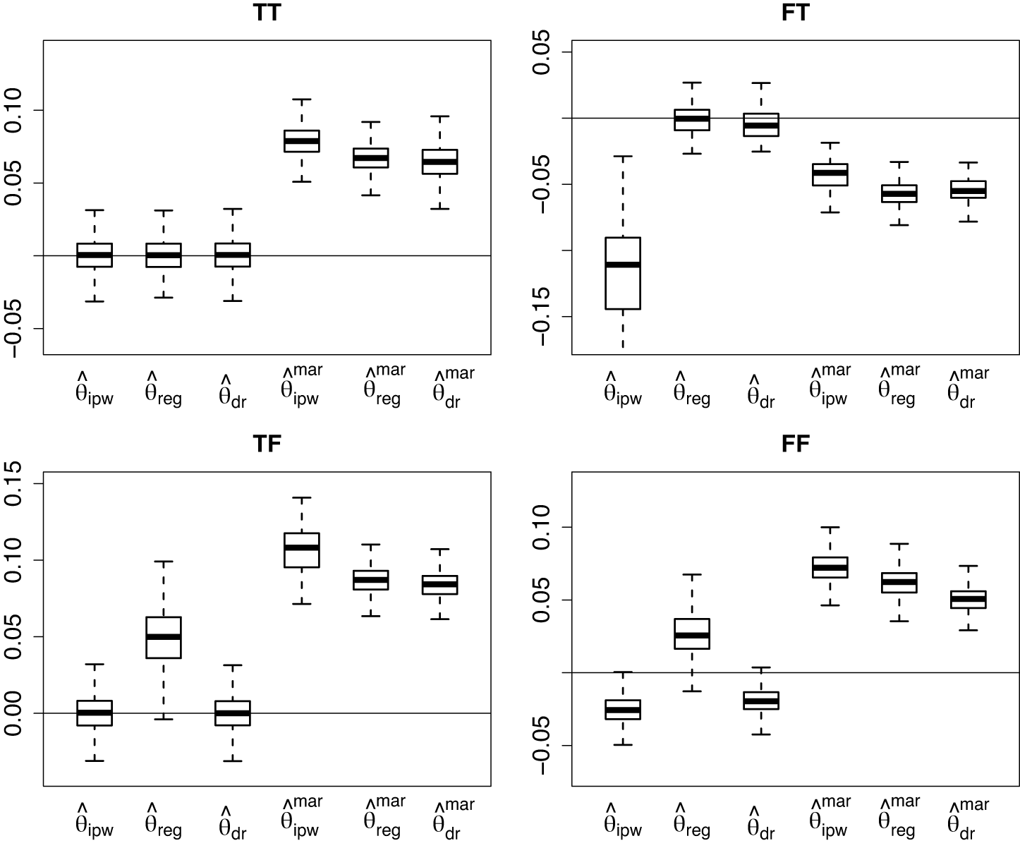


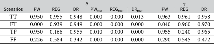

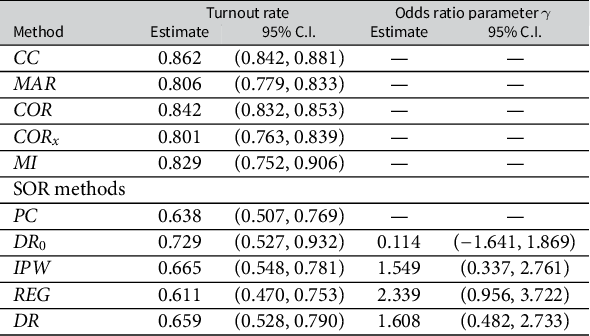


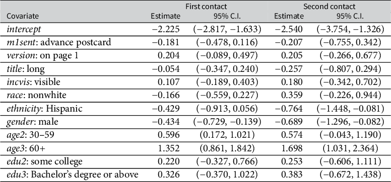
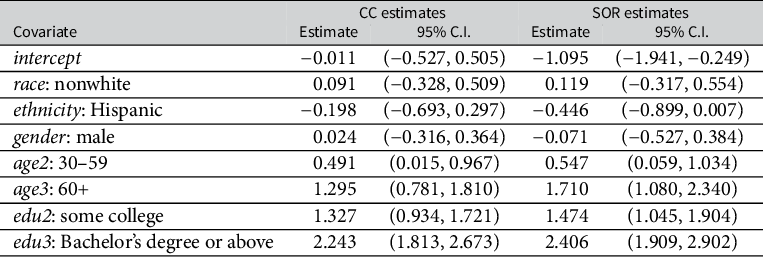
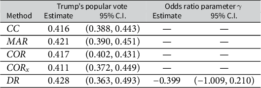


 Open access