





Introduction
Geothermal heat flux at the base of ice sheets (BGHF) is a critical boundary constraint on ice-sheet models because it plays a key role in the basal temperature and thermal gradients within glaciers (Pittard and others, Reference Pittard, Roberts, Galton-Fenzi and Watson2016). Accurate models of BGHF are necessary to predict subglacial melting rates, flow velocities in continental ice sheets and identify regions of extremely old ice (Larour and others, Reference Larour, Morlighem, Seroussi, Schiermeier and Rignot2012a; Liefferinge and Pattyn, Reference Liefferinge and Pattyn2013; Pittard and others, Reference Pittard, Roberts, Galton-Fenzi and Watson2016; Parrenin and others, Reference Parrenin2017). Despite the importance of BGHF, there are very few direct estimates aside from a few core sites (e.g. Parrenin and others, Reference Parrenin2017) and estimates made using subglacial lakes (Siegert and Dowdeswell, Reference Siegert and Dowdeswell1996).
Heat flux at the base of the Antarctic ice sheet is poorly constrained, leading many glacial modelers to use simple BGHF estimates to estimate temperature at the base of the Antarctic ice sheet (Llubes and others, Reference Llubes, Lanseau and Rémy2006; Larour and others, Reference Larour, Seroussi, Morlighem and Rignot2012b). Uncertainty in BGHF results in subglacial temperature models that cannot accurately predict subglacial melting. While more recent BGHF models derived from seismic tomography and Curie depth estimates are available (An and others, Reference An2015; Martos and others, Reference Martos2017; Lösing and others, Reference Lösing, Ebbing and Szwillus2020; Shen and others, Reference Shen, Wiens, Lloyd and Nyblade2020), these models are not of sufficient resolution to observe local thermal variations that may be significant to glacial processes (Liefferinge and Pattyn, Reference Liefferinge and Pattyn2013). These processes include the raising or lowering of the strain rate of ice (Goldsby and Kohlstedt, Reference Goldsby and Kohlstedt2001), the formation of fast sliding ice streams (Engelhardt, Reference Engelhardt2004) and the formation of subglacial lakes in regions not defined by basic 1-D thermal gradients (Llubes and others, Reference Llubes, Lanseau and Rémy2006). Furthermore, to estimate BGHF, these geophysical models rely on simple estimates of crustal heat production and thermal conductivity that are poorly constrained. In this study, we focus on the implications of shallow differences in thermal conductivity on temperature and heat flux at the ice–bedrock interface.
Heat moves from the lithosphere to the surface via the path of least resistance (Beardsmore and Cull, Reference Beardsmore and Cull2001), which is predominantly vertical due to the difference in temperature between the base of the lithosphere and the surface. Surface topography and lateral variations in composition cause the flow of heat to deviate from a straight path, resulting in a horizontal component of heat flux and creating local anomalies (Lees, Reference Lees1910; Lachenbruch, Reference Lachenbruch1968). A prior model for heat flux at the base of glaciers assumed the interface could be modeled as a topographic free surface (van der Veen and others, Reference van der Veen, Leftwich, von Frese, Csatho and Li2007). However, this assumption is physically incorrect because it ignores refraction of heat flux and temperature at the ice–bedrock interface as a result of a finite thermal conductivity of ice.
Thermal refraction distorts local thermal gradients in response to a contrast in thermal conductivity (Fig. 1). The effects of thermal refraction have been observed and accurately modeled within and around sedimentary basins (Stephenson and others, Reference Stephenson, Egholm, Nielsen and Stovba2009; Fuchs and Balling, Reference Fuchs and Balling2016). This refraction effect also has the potential to influence glacial and geothermal processes, as refraction locally focuses heat and temperatures relative to the surrounding area. This redistribution of heat affects viscosity due to its temperature sensitivity (Goldsby and Kohlstedt, Reference Goldsby and Kohlstedt2001) and the potential for subglacial melting. Furthermore, this phenomenon also accounts for local heat flux variations in the absence of subglacial topography.
Thermal refraction as a result of a conductivity contrast between ice and bedrock. The solid lines are for a 1-D temperature model where the underlying bedrock is more conductive than the ice (blue), less conductive (red) and equal (black). The dashed lines are computed for a 2-D temperature model through the center of a Gaussian-shaped valley (same models in Fig. 5). Because we do not factor in latent heat effects, temperatures above the melting point can be considered a melt potential (gray).

In this study, we demonstrate that, with or without subglacial topography, thermal refraction can affect the heat flux at the ice–bedrock interface, alluding to much warmer and cooler sections under the ice sheet. We suggest that thermal refraction creates regions of localized high temperature and heat flux anomalies that can raise melt potential, and may be responsible for subglacial lake formation.
Background
Topographic effect
The topographic method, originally theorized by Lees (Reference Lees1910) and later expanded by Lachenbruch (Reference Lachenbruch1968), accounts for surface heat flux into regions of low topography and away from high topography. van der Veen and others (Reference van der Veen, Leftwich, von Frese, Csatho and Li2007) proposed that the heat flux across the glacial–bedrock boundary can be described as a free surface and modeled using a topographic method, which they employed to describe the heat flux across the Petermann and Jakobshavn Isbræ subglacial boundaries in Greenland.
While air is very resistive, air currents – unlike ice – can convect thereby rapidly removing heat and creating a relatively constant temperature along the surface topography (i.e. the topographic effect). The result is a compression of isotherms in the vicinity of topographic depressions and associated increase in heat flux (Fig. 2). Beneath topographic highs, the opposite occurs, the distance between isotherms increases and heat flows away from the peak. The topographic model has been used by a number of glaciological studies and site planning. For example, in their recommendation for selection of an ice coring site, Passalacqua and others (Reference Passalacqua2018) suggest avoiding sites above subglacial valleys under the assumption that heat would be drawn into a valley and increasing the possibility of positive melting. In a separate study by Young and others (Reference Young2017), the authors assumed topography would increase the potential for subglacial lakes in regions of deeply incised topography.
A comparison of the topographic method (red) with the finite difference solution (blue) for a subglacial ridge and valley. The ice layer (light blue) is assigned a conductivity of 2 W m−1 K−1and the bedrock (light brown) is assigned a conductivity of 3 W m−1 K−1. The dashed lines and solid lines in (a) refer to the isotherms and heat flux lines, respectively. The topographic model is undefined in the ice whereas the isotherms extend across both layers in the finite difference model. (b) Basal heat flux anomalies for the topographic (red) and finite difference solutions (blue). The left axis displays the normalized heat flux anomaly (Eqn (6)) whereas the right axis displays the heat flux computed for regional heat flux of 40 mW m−2.
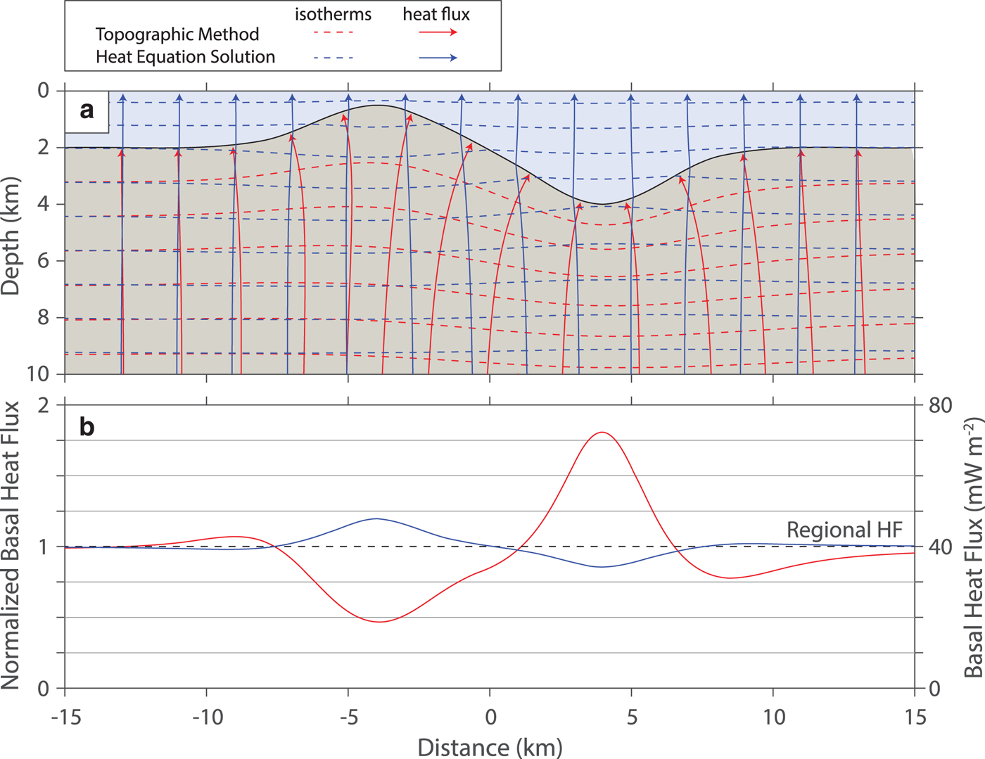
By using the topographic method, van der Veen and others (Reference van der Veen, Leftwich, von Frese, Csatho and Li2007) assumed the ice–bedrock boundary can be recast as Earth's free surface (Fig. 2), however this assumption is incorrect. For the topographic method to work in glacial systems, ice would need to be much more conductive than the bedrock or convect rapidly, both beyond what is practically possible. Earth materials – including ice – vary in thermal conductivity due to differences in composition, porosity and pore fluid. A conductivity contrast between ice and bedrock can result in thermal refraction of heat that can produce the opposite effect on heat flow above subglacial highs and valleys as predicted by the topographic method (Fig. 2). Therefore, thermal refractive effects must be considered for accurate glacial and ice-sheet models.
In this study, we revisit the basal heat flux in response to subglacial topography using the finite difference method, which can account for variations in thermal conductivity.
Thermal conductivity
Ice
The thermal conductivity of Antarctic ice varies considerably as a function of porosity and temperature (Pringle and others, Reference Pringle, Eicken, Trodahl and Backstrom2007). Pure ice at 0°C has a thermal conductivity of ~2.1 W m−1 K−1 and at −50°C (typical surface temperature in East Antarctica) ice is more conductive, 2.8 W m−1 K−1 (Paterson, Reference Paterson1994). In practice, the conductivity of glacial ice is lower than the pure ice limit as air bubbles in accumulating snow are trapped as the snow compacts into glacial ice. As snow compacts, it increases in both density and thermal conductivity (Eqns (9.3) and (9.4) in Paterson, Reference Paterson1994). Using density data from Kuivinen and Koci (Reference Kuivinen and Koci1982), we can estimate the upper and lower bounds of glacial ice thermal conductivity, which can be as low as 0.5 W m−1 K−1 near the surface and rapidly increases with depth to that of pure ice around 200 m (Fig. 3a). Observations of sea ice conductivity compiled by Pringle and others (Reference Pringle, Eicken, Trodahl and Backstrom2007) are consistent with this theoretical model. A complete set of equations to estimate the conductivity of ice with depth is provided in the Appendix.
(a) Models for the thermal conductivity of ice (see Appendix). (b) Distribution of thermal conductivities for selected igneous rock types (Jennings and others, Reference Jennings, Hasterok and Payne2019, and references therein). (c) Distribution of thermal conductivities for selected sedimentary rock types (Fuchs and others, Reference Fuchs, Schütz, Förster and Förster2013).

Bedrock
The vast array of rock compositions is associated with significant variations in thermal conductivity of about 5 W m−1 K−1 (Figs 3b, c). Porosity and pore fluid compositions further broaden the range of conductivities in shallow bedrock. Unweathered plutonic rocks have a relatively well-defined conductivity range from 1.8 W m−1 K−1 for alkali basalts up to 3.8 W m−1 K−1 for granites (Jennings and others, Reference Jennings, Hasterok and Payne2019). By contrast sedimentary rocks have much larger variations in conductivity ranging from 1 W m−1 K−1 for mudstones to 5.25 W m−1 K−1 for quartz-rich sandstones (Fuchs and others, Reference Fuchs, Schütz, Förster and Förster2013). This large conductivity range for sedimentary rocks is related to the large range of porosities and quartz fraction. Quartz has a conductivity of 6–8 W m−1 K−1 whereas most common rock-forming minerals have conductivities < 3 W m−1 K−1.
In general, most rock types will have thermal conductivities higher than that of ice and those with lower conductivities are likely to be easily eroded by moving ice. In Figure 3, we compare the thermal conductivity of ice with that of a few common igneous and sedimentary rocks. The median thermal conductivity of the rocks shown is similar to or above the asymptotic thermal conductivity of ice, but there are a significant number of rocks that have conductivity lower than ice. Therefore, it is important to consider the conductivity contrast between rock and ice in order to produce accurate models of heat flow.
Greenland and Antarctica are sufficiently large with lengthy and diverse tectonic histories (Harley and others, Reference Harley, Fitzsimons and Zhao2013; White and others, Reference White2016). Therefore, one can reasonably expect a very large range of rock types similar to what one may find on any other continent. There are some regions where sufficiently large exposures of rocks outcrop, generally near the coasts, that can be used to model the subsurface geology allowing one to produce accurate models of thermal conductivity. There are some subglacial basins beneath Antarctica where one can expect relatively low thermal conductivity sediments juxtaposed against crystalline rocks with significantly higher thermal conductivity. One may also find that crustal sutures are regions where there are significant contrasts in rock types and possibly conductivity. However, there are no thermal conductivity measurements specific to rocks exposed in Antarctica.
Some thermal studies estimate thermal conductivity using various mixing formulae in combination with modal mineralogy. Another possibility is the use of bulk geochemistry to estimate thermal conductivity (Jennings and others, Reference Jennings, Hasterok and Payne2019). Bulk geochemistry data are advantageous as it is often widely available where bedrock is accessible. While these techniques are physically sound and frequently accurate (e.g. Ray and others, Reference Ray2015; Chopra and others, Reference Chopra, Ray, Satyanarayanan and Elangovan2018; Fuchs and others, Reference Fuchs, Förster, Braune and Förster2018), they require in-depth knowledge of the bedrock and thus have limited utility for most sub-glacial heat flux studies.
In reality, the rock types beneath much of Greenland or Antarctica are unknown. When access to bedrock is not possible, empirically derived covariance relationships between thermal conductivity and other petrophysical parameters such as P-wave velocity and density may be used to estimate thermal conductivity (e.g. Hartmann and others, Reference Hartmann, Rath and Clauser2005; Sundberg and others, Reference Sundberg, Back, Ericsson and Wrafter2009). However, such regional settings are not geographically transferable as they typically depend on site-specific parameters that are often not discernible without access to bedrock samples. A recent study by Jennings and others (Reference Jennings, Hasterok and Payne2019) developed a model to estimate thermal conductivity from P-wave velocity from a global set of 340 non-porous igneous rocks,

with an accuracy of 0.31 W m−1 K−1. Therefore, it may be possible to remotely estimate the thermal conductivity of bedrock without direct access to the geology.
Because of the broad range of geologic environments and thermal conductivity contrasts possible beneath ice sheets, we have chosen to illustrate the range of refractive effects on simplified geologic structures rather than focus on any particular locality.
Methods
Topographic solution
The topographic method developed by Lees (Reference Lees1910) and Lachenbruch (Reference Lachenbruch1968) uses a series of planes and slopes to compute the topographic perturbation to the background thermal field. However, this method is cumbersome and more difficult to implement than an alternative formulation based on Fourier series proposed by Blackwell and others (Reference Blackwell, Steele and Brott1980). Both methods assume a homogeneous thermal conductivity medium and produce similar estimates for the topographic disturbance to the heat flow field. Therefore, due to its ease of use, we prefer the topographic method based on Fourier series.
The topographic effect on temperature at depth for a known temperature distribution along an uneven surface, T(x, 0), temperature can be computed by

at a distance x along a profile and a depth z relative to the surface (z(x) = 0), where Q is the regional heat flux defined in the absence of topography, k r is the thermal conductivity of bedrock, λ is the width of region of observation, and A n and B n are Fourier coefficients (Blackwell and others, Reference Blackwell, Steele and Brott1980). The Fourier coefficients can be determined by inversion of a surface temperature at a set of known or estimated points (Henderson and Cordell, Reference Henderson and Cordell1971). The local (topographically perturbed) heat flux, q, is then determined by Fourier's law applied to the equation above in both the horizontal ($\hat {{\bf x}}$ ) and vertical ($\hat {{\bf z}}$
 ) directions, i.e.

The topographic method is attractive because it does not rely on detailed information about the bedrock if the equations are recast in terms of the thermal gradient, Γ = Q/k r, such that the equations do not explicitly contain the thermal conductivity.
The topographic method fails to account for the presence of ice and as a result will not produce an accurate refractive effect. Therefore, we resort to solving the heat equation that incorporates a layer of ice over bedrock using a finite difference method. To demonstrate the impact of a glacial layer on the heat flux at the ice–bedrock interface, we solve the 2-dimensional, steady-state heat equation without sources,

where k and T are the conductivity and temperature, respectively, at a specific point in the medium. We solve this form of the thermal diffusion equation using successive over-relaxation applied to a finite difference approximation over a 2-D subglacial cross-section with cell sizes of ~0.01 × 0.01 km2 with the following boundary conditions:
• fixed surface temperature, T s(x);
• fixed temperature at the vertical boundaries consistent with 1-D model; and
• fixed heat flux, Q, on the lower boundary.
To reduce the number of iterations and shorten convergence time, we solve a coarse grid first and progressively double the resolution until the target resolution is attained. The convergence criteria is set to 1 × 10⁻³ °C for the maximum temperature change of any cell during an iteration. To estimate heat flux, we apply Fourier's Law by differentiating the temperature grid and multiplying by thermal conductivity. We then interpolate the temperature and heat flux at the ice-rock boundary.
To extend the utility of our calculations, we recast our results in terms of a non-dimensionalized temperature and heat flux. The use of non-dimensional quantities is independent of the regional heat flux and surface temperature chosen for the model and thus do not limit our results to the specific examples demonstrated in this study. The non-dimensionalized temperature, θ, and heat flux, Φ at the ice–bedrock boundary are given by


where T b and |q b| are the magnitude of temperature and heat flux at the boundary, and T b,1D and q b,1D are the boundary temperature and heat flux for the 1-D case associated with each vertical column across the section. For our models, q b,1D is equal to the regional heat flux, Q, and T b,1D = T s + Q h/k i, where h is the ice thickness.
In order to emphasize the effect of thermal refraction, we have made a number of assumptions to the heat flux equation. The above formulation ignores the influence of basal shear heating that is likely to dominate in regions with significant ice transport. In such cases, the geothermal heat flux contributions to the ice sheet are probably insignificant. We also ignore advection within the ice, which will affect the upper portion of the geotherm resulting in nearly isothermal temperatures at the surface (e.g. Dahl-Jensen and others, Reference Dahl-Jensen1998). As a result, the top of our models could be considered to begin at the point for which the ice has reached a conductive thermal profile. Advection near the base of thick ice may also have an effect and would normally be taken into account during modeling. We also ignore latent heat effects in instances where the models predict temperatures in excess of the melting point of ice (e.g. Fig. 1). Such temperatures can be considered as melt potential instead, where in reality, temperatures would be fixed to the melting temperature at the base of the ice and reducing temperatures within the overlying glacial column. Because we are simply demonstrating the effect of thermal refraction, it is the relative – not absolute – temperature difference that is important. The last assumption we make is that the crust contains negligible heat generation whereas continental crust contains significant radioactive heat generation that contributes to curvature in the geotherm (Chapman, Reference Chapman1986). However, the effect is small enough in the shallow Earth that it can be reasonably ignored.
Model geometries
To demonstrate how thermal refraction effects the flow of heat in glacial environments we construct the following models: (1) a Gaussian-shaped valley and (2) a subglacial geologic contact below a flat horizontal ice sheet. We have chosen these two basic geometries because they can be easily tailored to produce a wide range of common geologic and geomorphic features. To prevent boundary effects on calculations, model domains were typically set to approximately 10 times the width and depth of the subglacial topographic features.
Gaussian valley
A Gaussian-shaped sub-glacial valley is presented to illustrate the range of thermal refractive effects in response to changes in thermal conductivity and geometry (e.g. Fig. 4a). The valley is constructed by assigning a regional ice-sheet thickness, h, a width, w, and a depth, d (Fig. 4a). The ice is assigned a uniform thermal conductivity, k i, of 2 W m−1 K−1 and the bedrock conductivity is constant for each model.
Model setup and parameters used to model thermal refraction. Two classes of models are explored: (a) subglacial valley in a Gaussian shape and (b) subglacial contact beneath a flat subglacial surface.

Subvertical geological contact
Refraction also happens where there is no topography along the ice–bedrock interface when a geological contact juxtaposes rock types with differing thermal conductivity (Fig. 4b). To demonstrate this effect, we present a simple model for a geological contact below the ice. The model as shown in Figure 4b can be thought of as a fault-bounded sedimentary basin with a thickness, d, and an acute contact angle δ measured from the horizontal. In this case, there are two bedrock conductivities, one for the sedimentary basin, k s and one for the surrounding bedrock, k b.
Results
Gaussian valley
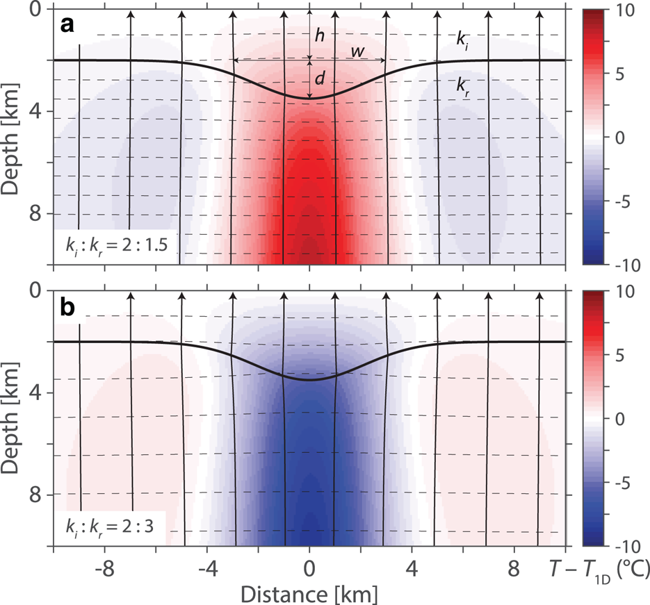
The results of the finite difference solution are presented in Figure 5 for a bedrock conductivity of 1.5 and 3 W m−1 K−1, respectively. When k i > k r, heat preferentially flows into the valley as it represents the easiest path to the surface (Fig. 5a). As a result, the isotherms bend away from the valley creating higher temperatures in the ice above the valley and lower temperatures in the bedrock below. However, relative to a series of one-dimensional vertical temperatures stitched across the profile, temperature is higher both above and below the valley (Fig. 6a). The valley flanks have anomalously low temperatures with slightly negative side lobes. The shape of the heat flux anomaly is similar to the temperature anomaly (Fig. 6b).
Thermal refraction due to a Gaussian-shaped valley. The models are computed for a thermal conductivity contrast of ice to rock, k i : k r, of (a) 2:1.5 and (b) 2:3. Geometric parameters h, w and d are used to define the ice thickness, valley width and valley depth, which are 2, 6 and 1.5 km, respectively. Isotherms are indicated by dashed lines and vector streamlines indicate the path of heat flow to the surface. The temperature anomaly is shown in the background, computed by subtracting the 1-D temperature field at each point along the profile from the model temperatures (numerator of Eqn (6)).
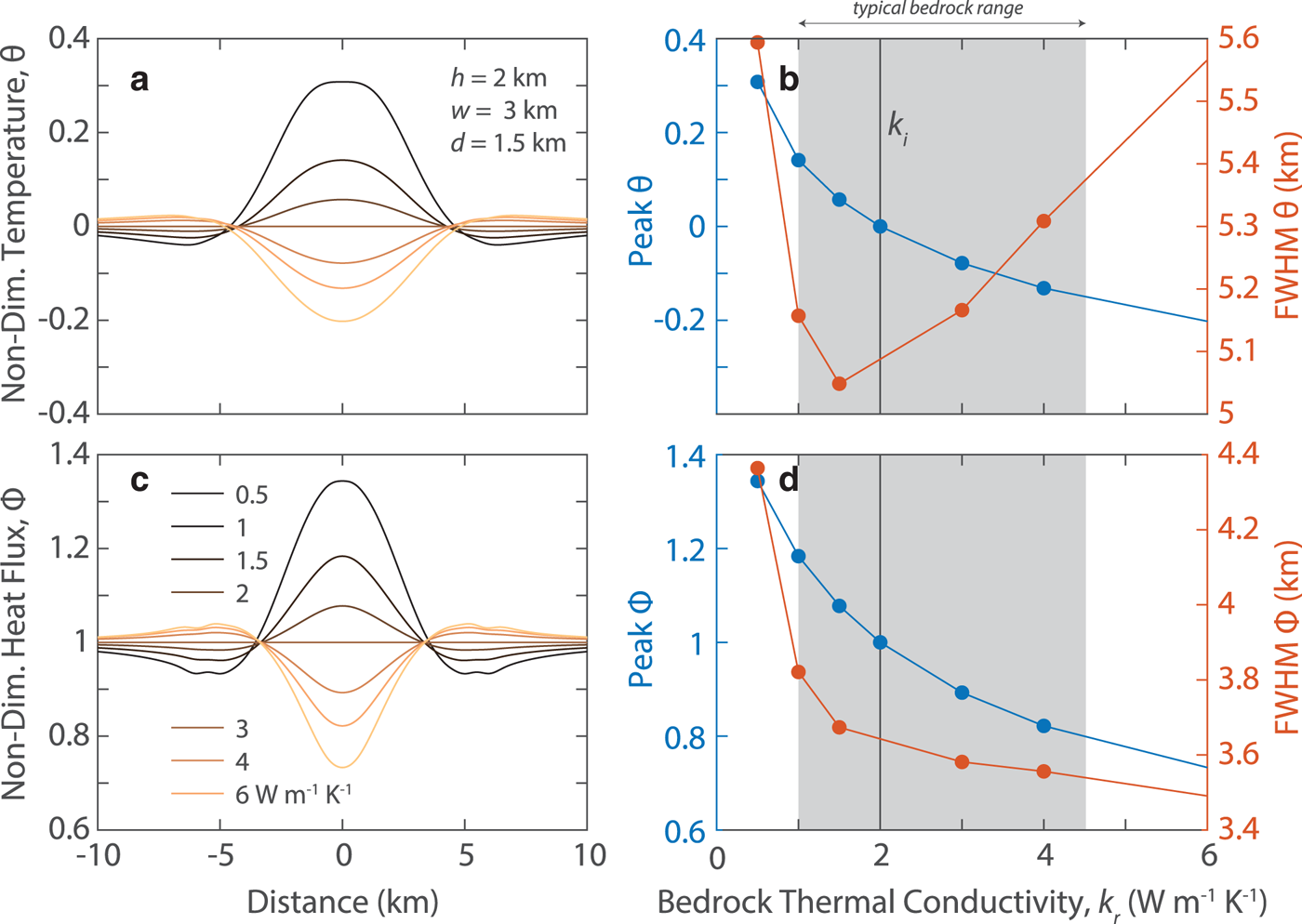
Basal temperature anomalies (a, b) and basal heat flux anomalies (c, d) across a Gaussian-shaped valley as a function of bedrock thermal conductivity. The models are computed for the same geometry in Figures 5 a, b. Profiles at the ice–bedrock interface. (c, d) The value of the central peak (blue) and full-width at half maximum (orange). The value of ice conductivity, k i, is indicated by the vertical line and gray field indicates the range of conductivity for most rocks (c, d). Non-dimensional temperature and heat flux definitions are given in Eqn ( 6). Because of a heat flux discontinuity at the boundary, the heat flux is estimated by averaging the flow just above and below the boundary to reduce numerical noise.
When the conductivity contrast is reversed, k i < k r, the heat flux and temperature anomalies both reverse polarity (Fig. 5). In this scenario, the isotherms bend toward the valley as heat flows around the valley.
Refraction can reduce or increase the difference between the valley flank and valley base temperatures, but temperatures will always be higher at the valley base than the flanks as a result of a positive thermal gradient with depth. However, the non-dimensionalized heat flux anomaly is related to an increase or decrease in temperature with respect to the vertical 1D temperature field, which preserves the sign of the absolute heat flux anomaly.
The magnitude of the basal temperature and basal heat flux anomalies vary smoothly as a function of the thermal conductivity contrast between the ice and rock (Fig. 6). For the bedrock conductivities chosen for this model, the basal temperature anomalies range from −0.2 to 0.3. The basal heat flux anomalies can vary between 0.7 and 1.3 as a fraction of the regional BGHF. However, this range is probably more extreme than most settings beneath thick ice, which are more likely to range from −0.15 to 0.15 for basal temperature anomalies and from 0.8 to 1.1 for basal heat flux anomalies (Figs 6b, d).
The geometry of the Gaussian basin has an effect on the basal thermal anomalies. We computed 112 separate models with varying bedrock conductivity, ice thickness, valley width and valley depth to examine the effect of geometry on the basal thermal anomalies (Fig. 7). An increase in ice thickness and valley width reduces the magnitude of the refraction effect. However, the reduction in non-dimensionalized magnitude is negligible as a function of ice thickness within the typical range for most rock types. In contrast to the other geometric parameters, an increase in valley depth results in an increase in the severity of the refractive effect.
Basal temperature anomalies (a, c, e) and basal heat flux anomalies (b, d, f) across a Gaussian-shaped valley as a function of bedrock thermal conductivity and model geometry. Geometry parameters are defined in Figure 5. Each pair of temperature heat flux plots are computed with geometry and ice conductivity given in Figure 5. The black contour in each plot identifies the estimated zero anomaly.

Subglacial geologic contact
For the subglacial model presented in Figure 8 with k b > k s, the heat preferentially flows around the basin near the subvertical contact with the bedrock. This contrast results in a decrease in heat flux at the western edge of the basin and an increase in heat flux through the bedrock to the west of the contact. Isotherms however, result in higher temperatures in the basin but lower than expected from a 1D model. On the bedrock side, temperatures are increased relative to a 1D model. Though the disturbances to the thermal field are largest below the ice, there is an effect on temperature and heat flux within the ice sheet itself.
Thermal refraction due to a geologic contact beneath an ice sheet. The model is computed for a thermal conductivity contrast of ice to the two bedrock layers, k i : k b : k s, of 2:3:2.2. Geometric parameters h, d and δ are used to define the ice thickness, basin depth and contact dip angle, which are 2 km, 3 km and 60°, respectively. Isotherms are indicated by dashed lines and vector streamlines indicate the path of heat flow to the surface. The temperature anomaly is shown in the background, computed by subtracting the 1-D temperature field at each point along the profile from the model temperatures (numerator of Eqn (6)).

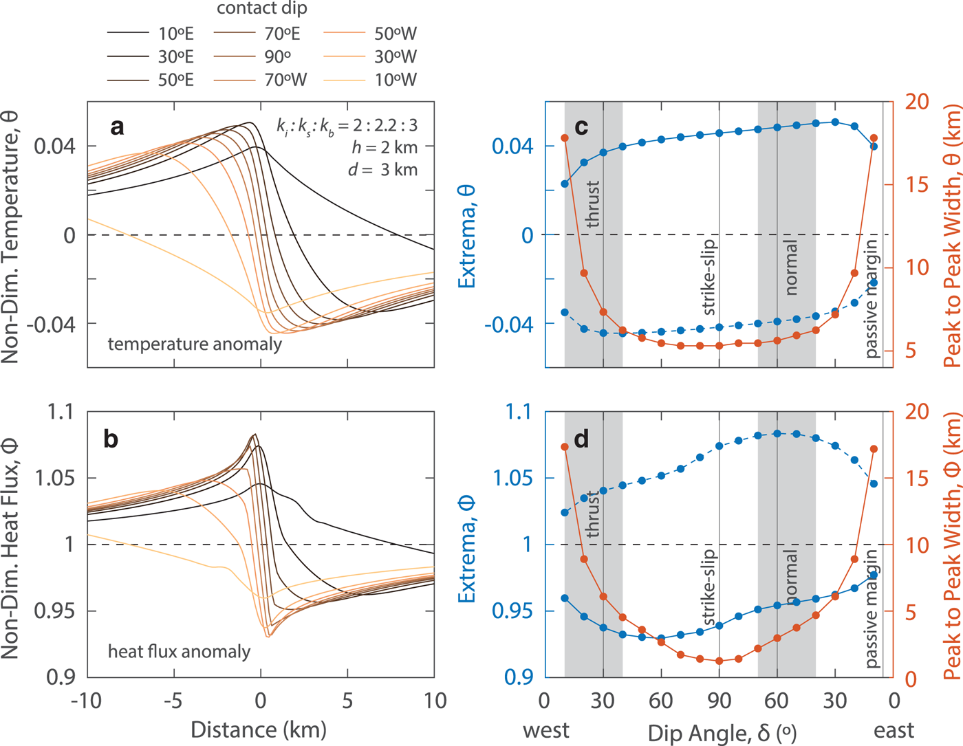
As with the valley model, model geometry has a significant effect on the thermal anomalies. In Figure 9, we compute the thermal anomalies for a variety of contact angles using the same conductivities and basin depth as in Figure 8. The anomalies are asymmetric as a result of the both the finite depth of the basin and the subvertical dip. The extrema slowly change with the dip angle except at low dip angles (<10°) that rapidly approach zero (Fig. 8). The peak to peak distance also increases dramatically at low angles (Figs 9c, d). The basal heat flux anomalies and basal temperature anomalies are as large for the fault model as similar bedrock conductivity models for the Gaussian valley.
Basal temperature anomalies (a, c) and heat basal flux anomalies (b, d) across a geologic contact as a function of contact dip angle. The geometry is defined in Figure 8, where dip angle is measured as an acute angle to the surface with dip direction denoted as to the east (right) or west (left). Although geologic contacts can be rotated into any angle through tectonic processes, we have labeled the common angles associated with unrotated fault types and passive margin slopes.
The conductivity ratio between the basin and bedrock determines the magnitude of the thermal anomalies, not the absolute conductivities. Figure 10 shows the results for 112 subglacial contact models computed with a range of basin and bedrock thermal conductivities. Lines of constant magnitude for both temperature and heat flux anomalies (colors in Fig. 10) follow lines of constant k s : k b ratio, which demonstrates that the magnitude of the refraction effect is independent of the absolute conductivities. For k s : k b ratios <1, the maximum basal temperature anomaly and basal heat flux anomaly are on the bedrock side of the contact whereas the maximum and minimum swap sides when k s : k b is >1, i.e. the positive anomaly is located on the conductive side of the contact.
Basal temperature anomalies (a, b) and basal heat flux anomalies (c, d) across a geologic contact as a function of bedrock and sedimentary basin conductivity. The geometry is shown in Figure 8. Normalized temperature (a, b) and heat flux (c, d) extrema for a geologic contact with 60° dip. Contours are drawn for conductivity ratios of basin (k s) to bedrock (k b). Ice conductivity is 2 W m−1 K−1 for both models. Extrema on the bedrock side of the contact (a, c) and basin side (b, d). The black contour in each plot identifies the estimated zero anomaly. Each pair of temperature heat flux plots are computed with geometry and ice conductivity given in Figure 8.

Discussion
Topographic vs finite difference solutions
To compare the topographic model and the finite difference solution, we have produced a subglacial topographic profile across a ridge and hill (Fig. 2). The topographic method is computed with a constant surface temperature as implied by the model produced by van der Veen and others (Reference van der Veen, Leftwich, von Frese, Csatho and Li2007), though it is unlikely to be true. Isotherms from the topographic method are expanded beneath the ridge and heat flux is decreased whereas below the valley isotherms are compressed and heat flux is increased (Fig. 2a). The overall topographic effect on heat flux predicts large local variations of nearly 50–175% compared to the regional heat flux (Fig. 2b).
The finite difference solution will be dependent upon the thermal conductivity of the ice and bedrock, but will result in a smaller disturbance to the heat flux field at the base of the ice. In Figure 2, we use a thermal conductivity contrast of 2:3 between the ice and bedrock layers. In this case, the polarity of the anomaly is reversed relative to the topographic solution and considerably smaller in magnitude, creating anomalies no larger than ±25%. If the conductivity contrast is reversed, the same polarity can be obtained for the finite difference solution, but the thermal conductivity contrast would need to be at least 10:1 to obtain similar magnitude anomalies as the topographic solution. Such a case can be easily rejected as geologically unrealistic.
The polarity of thermal anomalies computed using the topographic solution can be reversed only by two unrealistic scenarios: a negative regional heat flux or by imposing certain surface temperature profiles. A negative heat flux, heat flowing from the surface into the Earth, is generally unreasonable except as a result of diurnal and climatic warming – both extend less than a few 10's of meters into the subsurface and are transient. Changing the surface temperature profile is possible, but requires a priori knowledge. If the surface temperature is set properly, the topographic solution will be the same as the finite difference solution only when there are no subsurface variations in thermal conductivity. Because we rarely know the basal temperature along the glacier bed a priori, this is unrealistic.
The topographic solution applied to a subglacial boundary also fails to accurately predict basal heat flux anomalies in many geological settings. The finite difference solution predicts zero thermal anomalies when thermal conductivity of ice and bedrock are equal, irrespective of the bed topography (Fig. 7). The topographic solution will also not yield a thermal anomaly where there is no bed topography, but a lateral thermal conductivity contrast exists. As discussed above, the finite difference solution predicts significant thermal anomalies in such cases (Fig. 8).
Implications for ice viscosity and subglacial melting
Both the viscosity of ice sheets and the potential for melting are effected by temperature and heat flux anomalies created by thermal refractive effects. As our models predict basal temperature anomalies that extend into glaciers and ice sheets, we expect an effect change to viscosity and melt potential. For instance, glaciers weaken in response to heating (Perol and Rice, Reference Perol and Rice2015) and our models predict both heating and cooling in response to thermal refraction effects. As a result, we expect refraction to stabilize glaciers in some regions while weakening in others. While our discussion below focuses on the potential for melting, the effects have a broader effect on viscosity.
Our valley models suggest that subglacial melting is easier for some geometries and conductivity contrasts than others. Melting will always occur most readily at the base of a valley where temperatures are highest, but deep, narrow valleys where the thermal conductivity of the bedrock is less than ice will result in enhanced melting (Figs 1, 6, 7). Conversely, valleys where the bedrock conductivity is higher than the ice will result in a reduction of melt potential (Figs 1, 6). The latter model is in direct contrast to the predictions by the topographic method. Because thermal conductivity is generally greater in bedrock than ice, we suggest ice sheets will more likely be stabilized by topographic depressions (Fig. 2).
Though we have generally worked in non-dimensional units, we can place the magnitude of temperature and heat flux anomalies in context. In East Antarctica and Greenland where the ice is generally 2 km thick or above, 40–50 mW m−2 is a reasonable heat flow for similar aged terranes (Lucazeau, Reference Lucazeau2019), and for a bedrock conductivity of 3 W m−1 K−1 (θ = 0.1, ϕ = 0.9), the estimated heat flux anomaly is −4 to −5 mW m−2 and temperature anomalies 2–2.5 °C. For bedrock conductivities of 4 W m−1 K−1, the anomalies would be twice these values. While these numbers are not large, they could be sufficient to suppress melting and increase viscosity. Likewise, for conductivities lower than ice, the magnitudes will be similar, but opposite in sign.
Subglacial ridges have thermal anomalies opposite in polarity to subglacial valleys (Fig. 2). If melting were to occur, it would happen on the lower slopes of the high topography where thermal conductivity of the bedrock is less than the ice. However, the potential is likely to be low because the basal temperature anomaly side lobes have relatively small magnitudes.
Whereas melting is more likely in some valley scenarios, the mere presence of a subglacial geologic contact raises the melt potential even in the presence of no subglacial topography. A positive temperature anomaly is created irrespective of a higher thermal conductivity in the bedrock or basin, always creating the positive anomaly on the conductive side of a contact (Figs 10a, b). Furthermore, the magnitude of the temperature anomaly is relatively constant for all but shallow dip angles <20°, raising the potential for melting under a wide variety of geometries (Fig. 9). Such short wavelength variations in viscosity could result in folding of the ice sheet as it flows over such contacts (Bons and others, Reference Bons2016).
There is a potentially large difference in the spatial scale of melting and viscosity contrasts for the cases discussed above. Melting of ice beneath topographic lows is likely to be constrained spatially relative to a narrow region at the base of a valley (Fig. 6). Next to topographic highs, the spatial scale of broader but likely to be small in magnitude. Above geologic contacts, temperatures can remain significantly elevated for relatively large distances >10 km across strike on the high conductivity side (Fig. 9).
In most cases, the refraction effect will occur in regions where melting will not occur but viscosity will still be affected. In regions where melting occurs, our temperature estimates will be incorrect because melting will keep temperatures fixed at the melting point. In such cases, the melt rate can be estimated from the difference between the estimated BGHF and the heat flux at the surface,

where ΔT e is the excess temperature (i.e. estimated temperature anomaly above the ice's melting point at the base of the ice sheet), k i and ρi are the conductivity and density of the ice, h is the thickness of the ice sheet, and L is the latent heat.
Conclusions
We demonstrate the effect of heat refraction at the base of ice sheets in the presence of subglacial topography and above geological contacts. Previously proposed topographic-based models for heat flux across a subglacial boundary are physically incorrect as they make incorrect assumptions about the thermal conductivity of ice. In many cases – specifically where bedrock is more conductive than ice – heat flux and temperature will be reduced above topographic depressions, the opposite as predicted by the topographic effect. Thus, it is necessary that future thermal model of ice sheets incorporates lateral variations in thermal conductivity and the resulting thermal refractive effect. Thermal refraction can occur over spatial scales smaller than resolvable by remote-sensing estimates (e.g. seismic and Curie depth), but create heat flux and temperature anomalies sufficient to create subglacial melting. Subglacial melt potential may actually be decreased in valleys with thermally conductive bedrock relative to the overlying ice sheet. Changes in melt potential can increase, and viscosity decrease, on the conductive side of geologic contacts even when bed topography is flat. Likewise, ice viscosity is affected by thermal refraction of heat and therefore may influence ice flow velocities near geologic contacts and subglacial topographic features. While our models of ice sheets are simplistic, they illustrate the need to include refractive effects created by realistic geology into future glacial models. Including thermal refractive effects will improve the prediction of subglacial melting and ice viscosity where heat flux is dominated by geothermal heat flux rather than shear heating at the bed. We suggest that contrary to previous studies, topographic depressions may be regions where thick ice is more stable than previously assumed. The implications in this study are not limited to glacial environments but are applicable to any environment that contains variations in thermal conductivity.
Acknowledgements
We thank the Editor Bernd Kulssa, Lenneke Jong and an anonymous reviewer for their constructive comments that helped improved earlier versions of the manuscript. S.W. is supported by the Australian Government Research Training Program Scholarship. D.H. is supported by the Australian Government through the Australian Research Council's Discovery Projects funding scheme (project DP180104074).
Appendix
To compute the conductivity depth relationships shown in Figure 3a, we use the equation from Paterson (Reference Paterson1994),

where k i is the conductivity of pure ice, ρ i is the density of pure ice, and ρ is the observed density of ice at depth. The thermal conductivity of pure ice can be estimated using the relation by Paterson (Reference Paterson1994),

where T is temperature in degrees Celsius. The density of pure ice is given by

where αV is the thermal expansivity of ice, 112 × 10−6 K−1. The temperature can be determined from ice cores. For Figure 3a, we use the South Pole temperature profile as reported by Price and others (Reference Price2002),

where z is given in meters. The observed density of ice has been determined on a separate core by Kuivinen and Koci (Reference Kuivinen and Koci1982),

with z in meters.


 Open access

