

1 INTRODUCTION
Bilateral bargaining is one of the most important forms of trade. Despite there has been a large literature of bargaining in theory and in laboratory experiments over the past 60 years, we have seen a burst of empirical investigations of bargaining only in the past decade. This surge is mainly due to the increasing availability of bargaining data to the academic community. For instance, online bargaining interaction data from eBay’s best offer platform have been studied by Backus et al. (Reference Backus, Blake, Larsen and Tadelis2020) to document some facts consistent with bargaining theory by using some reduced form approach. Similarly, Larsen (Reference Larsen2021) utilizes wholesale used-auto auctions data to examine ascending auctions followed by bargaining under minimal assumptions of rational behavior. Finally, data on union-management negotiations collected by Treble (Reference Treble1990) provide reduced form evidence regarding conciliation board negotiations in the historical British coal industry. In this article, we study the identification and estimation of the structural double auction model which explicitly characterizes the bargaining process between buyer and seller. It is therefore a good alternative to the Nash bargaining framework.
A bargaining framework with two-sided incomplete information allows for inefficient outcome which occurs in real-world trade but is excluded by a framework with complete information. As an influential candidate of the former, the double auction with bargaining (or k-double auction) considers linear strategies for both the buyer and the seller. The linearity of the strategies has been confirmed by experimental studies (see, e.g., Radner and Schotter, Reference Radner and Schotter1989). This article nonparametrically identifies and estimates the double auction model with bargaining. Our framework can be used to recover the updated value distributions of the buyer and the seller based on the last round of bids, since previous rounds of bids are usually used to reveal limited information about the value of the reservation. For instance, our method can be employed to estimate the buyer’s and the seller’s (most updated) value distributions by using the last round of offers from the bargaining data of eBay’s best offer platform (or wholesale used-auto auctions, or union-management negotiations).
This article contributes to the literature of noncooperative bargaining games with incomplete information. On the theoretical side, such games have been extensively studied since Chatterjee and Samuelson (Reference Chatterjee and Samuelson1983). In addition, there is also a large experimental literature that examines the theoretical properties of bargaining with incomplete information (see, e.g., Radner and Schotter, Reference Radner and Schotter1989, among others). Empirically, there is a fast growing literature to investigate the role of asymmetric information in bargaining.Footnote 1 See Larsen (Reference Larsen2021) for wholesale used-auto market and Keniston (Reference Keniston2011) for local autorickshaw transportation. Our article belongs to the second research line (of the structural approach) and provides an empirical methodology to use the data on offers and asks at the last round of the bargaining process to estimate the updated valuation distributions of both participating parties. Our method can be applied to field data to quantify ex ante and ex post inefficiency introduced by private information (see Satterthwaite and Williams, Reference Satterthwaite and Williams1989).
Our article is also related to the literature that examines nonparametric identification and estimation of one-sided auctions. This work was pioneered by Guerre, Perrigne, and Vuong (Reference Guerre, Perrigne and Vuong2000) for the identification and estimation of first-price auctions, and has been followed by many other papers. For comprehensive surveys, see Athey and Haile (Reference Athey, Haile, Heckman and Leamer2007), Hendricks and Porter (Reference Hendricks and Porter2007), Hickman, Hubbard, and Sağlam (Reference Hickman, Hubbard and Sağlam2012), Gentry et al. (Reference Gentry, Hubbard, Nekipelov and Paarsch2018), Perrigne and Vuong (Reference Perrigne and Vuong2019), and Hortaçsu and Perrigne (Reference Hortaçsu and Perrigne2021). In the identification part, we generalize the Guerre et al.’s (Reference Guerre, Perrigne and Vuong2000) nonparametric identification strategy to the double auction setup. The model primitives are shown to be partially identified when only transacted bids are available, but to be point-identifiable when the failed bids are also available. Our identification results are hence similar to Gentry and Li (Reference Gentry and Li2014), who obtained constructive bounds on model fundamentals which collapse to point identification when available entry variation is continuous in auctions with selective entry.Footnote 2 There are other papers obtaining partial identification in the context of one-sided auctions (see, e.g., Haile and Tamer, Reference Haile and Tamer2003; McAdams, Reference McAdams2008; Tang, Reference Tang2011; Aradillas-López, Gandhi, and Quint, Reference Aradillas-López, Gandhi and Quint2013; Komarova, Reference Komarova2013; Chen et al., Reference Chen, Gentry, Li and Lu2020). However, compared to this research line, we consider identification in a different auction setting (namely, double auctions with bargaining) that introduces not only asymmetric information but also asymmetric bidding strategies.Footnote 3 In the estimation part, our article is closely related to Hickman and Hubbard (Reference Hickman and Hubbard2014) who adapted the bias correction method of Zhang, Karunamuni, and Jones (Reference Zhang, Karunamuni and Jones1999) and Karunamuni and Zhang (Reference Karunamuni and Zhang2008) to correct the boundary bias of the two-step value density estimator, which was first proposed by Guerre et al. (Reference Guerre, Perrigne and Vuong2000), of (one-sided) first-price auctions. Their bias correction approach (and most other related approaches) needs to introduce additional tuning parameters for data modification and to know the true boundary location for defining the estimators and asymptotic analysis. In contrast, we apply Cattaneo, Jansson, and Ma’s (Reference Cattaneo, Jansson and Ma2020) local polynomial density estimators to correct both boundary and interior biases of bid and value densities, which exist in the equilibrium outcome of our double auction model. Our method is easy-to-implement and fully boundary adaptive. It introduces only one tuning parameter and does not need the knowledge of true support boundaries for estimator definition and asymptotic results.
In view of the preceding results, we consider nonparametric identification and estimation of double auction with bargaining. First, in addition to characterizing all the restrictions on the observables (i.e., bid distributions) imposed by the theoretical double auction model with bargaining, we establish the point identification of model primitives (i.e., value distributions) from the observables in the case where all bids are observed. In the case when only transacted bids are observed,Footnote 4 we provide a sharp identified set of bidders’ value distributions (in Theorem 4). We show that, in the latter case, the conditional distributions of bidders’ valuations given positive (conditional) probability of trade are point identified. Second, we propose the (boundary and interior) bias-corrected two-step estimators of the buyer’s and the seller’s value densities. In a double auction setting, we show that our estimators achieve the optimal convergence rate. Third, using Monte Carlo experiments, we show that it is important to implement bias correction (especially bias correction in the interior of the support) in the two-step estimation of value densities. In particular, we show that, without bias correction, the statistical inference is almost infeasible, not only on the boundaries but also in the interior.
The remainder of this article is organized as follows. In Section 2, we present the sealed bid double auction model with bargaining and characterize its equilibrium. Section 3 then studies the identification of private value distributions. In Section 4, we estimate both the bid and the value densities with bias correction and establish their uniform convergence rates. Section 5 uses Monte Carlo experiments to illustrate the finite sample performance of our estimators. Section 6 concludes the article. Appendix A collects the proofs of our main results in the text. Supplemental Material contains some additional results (as well as their proofs).
2 THE k-DOUBLE AUCTION MODEL
We consider a k-double auction in which a single and indivisible object is auctioned between a buyer and a seller. Each of them simultaneously submits a bid. If the buyer’s offer is no lower than the seller’s request, a transaction is made at a price of their weighted average, that is, at a price $ p(B,S) = k B+(1-k) S, $
where k is a constant in
$ p(B,S) = k B+(1-k) S, $
where k is a constant in $[0,1]$
, B is the buyer’s offer, and S is the seller’s request. Otherwise, there is no transaction. The buyer has a value V for the auctioned object, and the seller has a reservation value C. Consequently, the buyer’s payoff is
$[0,1]$
, B is the buyer’s offer, and S is the seller’s request. Otherwise, there is no transaction. The buyer has a value V for the auctioned object, and the seller has a reservation value C. Consequently, the buyer’s payoff is $V-p(B,S)$
and the seller’s payoff is
$V-p(B,S)$
and the seller’s payoff is $p(B,S)-C$
if a trade occurs; their payoffs are zero otherwise. Each of them does not know the valuation of her opponent, but only knows that it is drawn from a distribution
$p(B,S)-C$
if a trade occurs; their payoffs are zero otherwise. Each of them does not know the valuation of her opponent, but only knows that it is drawn from a distribution $F_j (j=C,V)$
. Distributions
$F_j (j=C,V)$
. Distributions $F_V$
and
$F_V$
and $F_C$
and the payment rule are all common knowledge between the buyer and the seller.
$F_C$
and the payment rule are all common knowledge between the buyer and the seller.
Notice that the weight k measures the bargaining power of the buyer and the seller: the larger k is, the stronger (or weaker) the bargaining power of the buyer (or seller). In particular, the case of $k = 1$
(resp.
$k = 1$
(resp. $k = 0$
) corresponds to the buyer (resp. seller) having all the bargaining power.
$k = 0$
) corresponds to the buyer (resp. seller) having all the bargaining power.
We impose the following assumption on the private values and their distributions.
Assumption A. (i) V and C are independent. (ii) $F_V$
and
$F_V$
and $F_C$
are twice continuously differentiable with densities
$F_C$
are twice continuously differentiable with densities $f_V$
and
$f_V$
and $f_C$
on
$f_C$
on $[\underline {v},\overline {v}]\subset \mathbb {R}_+$
and
$[\underline {v},\overline {v}]\subset \mathbb {R}_+$
and $[\underline {c},\overline {c}]\subset \mathbb {R}_+$
, respectively. In addition,
$[\underline {c},\overline {c}]\subset \mathbb {R}_+$
, respectively. In addition, $f_V(v)\geq \alpha _V>0$
for all
$f_V(v)\geq \alpha _V>0$
for all $v\in [\underline {v},\overline {v}]$
;
$v\in [\underline {v},\overline {v}]$
; $f_C(c)\geq \alpha _C>0$
for all
$f_C(c)\geq \alpha _C>0$
for all $c\in [\underline {c},\overline {c}]$
.
$c\in [\underline {c},\overline {c}]$
.
Under Assumption A, the private value of the seller is independent of the buyer’s, and the value distributions are twice continuously differentiable with densities being bounded away from zero on compact supports. Similar assumption has been adopted by most theoretical papers on double auctions with bargaining (see, e.g., Satterthwaite and Williams, Reference Satterthwaite and Williams1989).
We also impose the following restriction on the supports of $F_V$
and
$F_V$
and $F_C$
.
$F_C$
.
Assumption B. The supports of $F_V$
and
$F_V$
and $F_C$
satisfy
$F_C$
satisfy $\underline {c}<\overline {v}$
.
$\underline {c}<\overline {v}$
.
This assumption requires that the buyer’s maximum value must be higher than the seller’s minimum cost. It rules out the trivial case of $\overline {v}\leq \underline {c}$
in which there is zero probability of trade in any equilibrium. The special cases of such a support condition have been commonly adopted by the theoretical double auction literature (see, e.g., Leininger, Linhart, and Radner, Reference Leininger, Linhart and Radner1989).
$\overline {v}\leq \underline {c}$
in which there is zero probability of trade in any equilibrium. The special cases of such a support condition have been commonly adopted by the theoretical double auction literature (see, e.g., Leininger, Linhart, and Radner, Reference Leininger, Linhart and Radner1989).
Denote by $\beta _B: [\underline {v},\overline {v}]\to \mathbb {R}_+$
and
$\beta _B: [\underline {v},\overline {v}]\to \mathbb {R}_+$
and $\beta _S: [\underline {c},\overline {c}]\to \mathbb {R}_+$
the buyer’s and seller’s strategies, respectively. Let
$\beta _S: [\underline {c},\overline {c}]\to \mathbb {R}_+$
the buyer’s and seller’s strategies, respectively. Let $b=\beta _B(v)$
denote the bid of a buyer with realized private value v under strategy
$b=\beta _B(v)$
denote the bid of a buyer with realized private value v under strategy $\beta _B$
. Then, the expected profit of the buyer given the seller’s strategy is
$\beta _B$
. Then, the expected profit of the buyer given the seller’s strategy is
 $$ \begin{align} \pi_B(b,v)=\begin{cases} \displaystyle \int_{\underline{s}}^b [v-p(b,s)]\,\mathrm{d} G_S(s)=\int_{\underline{s}}^b [v-kb-(1-k)s]\,\mathrm{d} G_S(s), & \text{if } b\geq\underline{s},\\ 0, & \text{if } b<\underline{s}, \end{cases} \end{align} $$
where $G_S$
is the distribution function of the seller’s bid and
$G_S$
is the distribution function of the seller’s bid and $\underline {s}$
is the lower end point of its support. Similarly, let
$\underline {s}$
is the lower end point of its support. Similarly, let $s=\beta _S(c)$
denote the request of a seller with realized private reservation value c under strategy
$s=\beta _S(c)$
denote the request of a seller with realized private reservation value c under strategy $\beta _S$
. Then, the expected profit of the seller given the buyer’s strategy is
$\beta _S$
. Then, the expected profit of the seller given the buyer’s strategy is
 $$ \begin{align} \pi_S(s,c)=\begin{cases} \displaystyle \int_s^{\overline{b}} [p(b,s)-c]\,\mathrm{d} G_B(b)=\int_s^{\overline{b}} [kb+(1-k)s-c]\,\mathrm{d} G_B(b), & \text{if } s\leq\overline{b},\\ 0, & \text{if } s>\overline{b}, \end{cases} \end{align} $$
where $G_B$
is the distribution function of the buyer’s bid and
$G_B$
is the distribution function of the buyer’s bid and $\overline {b}$
is the upper end point of its support.
$\overline {b}$
is the upper end point of its support.
We adopt the Bayesian Nash equilibrium (BNE) concept throughout.
Definition 1 (Best Response).
A buyer strategy $\beta _B$
is the best response to
$\beta _B$
is the best response to $\beta _S$
if, for any buyer strategy
$\beta _S$
if, for any buyer strategy $\tilde \beta _B: [\underline v, \overline v]\rightarrow \mathbb R_+$
and each value
$\tilde \beta _B: [\underline v, \overline v]\rightarrow \mathbb R_+$
and each value $v\in [\underline v,\overline v]$
,
$v\in [\underline v,\overline v]$
, $\pi _B(\beta _B(v),v)\geq \pi _B(\tilde \beta _B(v),v)$
. The seller’s best response is defined in an analogous way.
$\pi _B(\beta _B(v),v)\geq \pi _B(\tilde \beta _B(v),v)$
. The seller’s best response is defined in an analogous way.
Definition 2 (Bayesian Nash Equilibrium).
A strategy profile $(\beta _B,\beta _S)$
constitutes a BNE if
$(\beta _B,\beta _S)$
constitutes a BNE if $\beta _B$
and
$\beta _B$
and $\beta _S$
are the best responses to each other.
$\beta _S$
are the best responses to each other.
Similar to other bargaining models under incomplete information, the BNE is not unique in our k-double auction model (with bargaining). This is considerably different from an auction model, which has a unique BNE within the symmetric independent private value paradigm. Thus, we exclude some irregular equilibria and focus on those which are well behaved as described in Chatterjee and Samuelson (Reference Chatterjee and Samuelson1983). Precisely, we impose the following restrictions on the equilibrium.
Assumption C (Regular Equilibrium).
The equilibrium strategy profile $(\beta _B,\beta _S)$
satisfies:
$(\beta _B,\beta _S)$
satisfies:
-
A1. $\beta _B$
and
$\beta _S$
are continuous on their whole domains;
$\beta _B$
and
$\beta _S$
are continuous on their whole domains; -
A2.
$\beta _B$
is continuously differentiable with positive derivative on
$[\underline {s},\overline {v}]$
if
$\underline {s}<\overline {v}$
;
$\beta _S$
is continuously differentiable with positive derivative on
$[\underline {c},\overline {b}]$
if
$\underline {c}<\overline {b}$
; -
A3.
$\beta _B(v)=v$
if
$v\leq \underline {s}$
;
$\beta _S(c)=c$
if
$c\geq \overline {b}$
.


We say that an equilibrium satisfying Assumption C is regular. Assumption C basically restricts us to strictly monotone and (piecewise) differentiable strategy equilibria that are quite intuitive in bilateral k-double auctions. Furthermore, the regularity conditions of the equilibrium strategy in Assumption C imply that the value densities $f_V(\cdot )$
and
$f_V(\cdot )$
and $f_C(\cdot )$
are continuous and bounded away from zero. As demonstrated by Satterthwaite and Williams (Reference Satterthwaite and Williams1989, Thm. 3.2), there exists a continuum of regular equilibria when
$f_C(\cdot )$
are continuous and bounded away from zero. As demonstrated by Satterthwaite and Williams (Reference Satterthwaite and Williams1989, Thm. 3.2), there exists a continuum of regular equilibria when $k\in (0,1)$
and
$k\in (0,1)$
and $[\underline {v},\overline {v}]=[\underline {c},\overline {c}]=[0,1]$
.Footnote
5
Following most of the empirical studies in game theory, we adopt the following equilibrium selection mechanism when multiple regular equilibria exist.
$[\underline {v},\overline {v}]=[\underline {c},\overline {c}]=[0,1]$
.Footnote
5
Following most of the empirical studies in game theory, we adopt the following equilibrium selection mechanism when multiple regular equilibria exist.
Assumption D. In all observed auctions, buyers and sellers play the same regular equilibrium.
The same regular equilibrium of Assumption D means a common pair of regular equilibrium strategy functions across observed auctions. If there are multiple regular equilibria across observed auctions according to an equilibrium selection rule, then the distribution of all observed bids will be a mixture of multiple equilibrium bid distributions following the selection rule. In this case, we will need to identify the equilibrium selection mechanism besides the value distributions.
The following lemma characterizes some basic properties of the equilibrium strategy profile.
Lemma 1. Under Assumptions A–C, for any equilibrium $(\beta _B,\beta _S)$
,
$(\beta _B,\beta _S)$
,
-
(i) when
$v>\underline {s}$
,
$\beta _B(v)\leq v$
with strict inequality if
$k>0$
; -
(ii) when
$c<\overline {b}$
,
$\beta _S(c)\geq c$
with strict inequality if
$k <1$
.


Proof. See Appendix A.1.
Note that the conclusion of Lemma 1 holds for any BNE (i.e., not only for regular BNE). With Condition A3 of Assumption C, it implies that, in regular equilibrium, the buyer will never bid higher than her private value, and the seller will never bid lower than her private value. In the special case of $k=1/2$
, Leininger et al. (Reference Leininger, Linhart and Radner1989) constructed a lemma similar to our Lemma 1.
$k=1/2$
, Leininger et al. (Reference Leininger, Linhart and Radner1989) constructed a lemma similar to our Lemma 1.
3 NONPARAMETRIC IDENTIFICATION
We study the nonparametric identification of private value distributions in two cases which differ in the degree of available data. In the first case, researchers can observe both the transacted bids and the bids where no transaction takes place.Footnote 6 In the second case, researchers can only observe the transacted bids.
3.1 Identification of Bargaining Power Parameter k
We first identify the bargaining power parameter k. The value of k can be recovered by using additional information on the transaction price, given that the transacted bids are observed. For example, when the mean transaction price is observed, the parameter k is determined by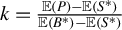 $k=\frac {\mathbb {E}(P)-\mathbb {E}(S^*)}{\mathbb {E}(B^*)-\mathbb {E}(S^*)}$
since
$k=\frac {\mathbb {E}(P)-\mathbb {E}(S^*)}{\mathbb {E}(B^*)-\mathbb {E}(S^*)}$
since $\mathbb {E}(P)=k\mathbb {E}(B^*)+(1-k)\mathbb {E}(S^*),$
where
$\mathbb {E}(P)=k\mathbb {E}(B^*)+(1-k)\mathbb {E}(S^*),$
where $(B^*,S^*)$
are the bids transacted.
$(B^*,S^*)$
are the bids transacted.
Alternatively, k can be identified by using a quantile of the transaction price. This quantile approach is useful when the mean transaction price $\mathbb {E}(P)$
is not available. For example, we cannot recover the mean transaction price if the transaction prices are censored by some threshold value from above or below. Nevertheless, we can still recover a transaction price quantile in this case. Let
$\mathbb {E}(P)$
is not available. For example, we cannot recover the mean transaction price if the transaction prices are censored by some threshold value from above or below. Nevertheless, we can still recover a transaction price quantile in this case. Let $\Psi _k(p)$
be the transaction price distribution function, where the subscript k indicates that the value of this function could also depend on the price weight k. We can express the transaction price distribution
$\Psi _k(p)$
be the transaction price distribution function, where the subscript k indicates that the value of this function could also depend on the price weight k. We can express the transaction price distribution $\Psi _k(p)$
in terms of the distribution of transacted bids as follows: (i) when
$\Psi _k(p)$
in terms of the distribution of transacted bids as follows: (i) when $0<k<1$
, we haveFootnote
7
$0<k<1$
, we haveFootnote
7
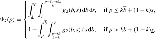 $$ \begin{align} \Psi_k(p)=\begin{cases} \displaystyle\int_{\underline{s}}^p \displaystyle\int_s^{\frac{p-(1-k)s}{k}} g_2(b,s)\,\mathrm{d} b\,\mathrm{d} s, & \text{if } p\le k\overline{b}+(1-k)\underline{s},\\[2ex] 1-\displaystyle\int_p^{\overline{b}} \displaystyle\int_{\frac{p-kb}{1-k}}^b g_2(b,s)\,\mathrm{d} s\,\mathrm{d} b, & \text{if } p> k\overline{b}+(1-k)\underline{s}, \end{cases} \end{align} $$
where $g_2(b,s) = g(b,s) / \Pr (\underline {s} \leq S \leq B\leq \overline {b})$
is the joint density of transacted bids; (ii) when
$g_2(b,s) = g(b,s) / \Pr (\underline {s} \leq S \leq B\leq \overline {b})$
is the joint density of transacted bids; (ii) when $k=0$
,Footnote
8
$k=0$
,Footnote
8
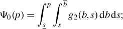 $$ \begin{align} \Psi_0(p)=\int_{\underline{s}}^p\int_s^{\overline{b}} g_2(b,s)\,\mathrm{d} b\,\mathrm{d} s; \end{align} $$
and (iii) when $k=1$
,
$k=1$
,
 $$ \begin{align} \Psi_1(p)=\int_{\underline{s}}^p\int_{\underline{s}}^b g_2(b,s)\,\mathrm{d} s\,\mathrm{d} b=\int_{\underline{s}}^p \int_s^p g_2(b,s)\,\mathrm{d} b\,\mathrm{d} s. \end{align} $$
The next lemma is the key to identify k using a transaction price quantile. It establishes the monotonicity of the transaction price distribution $\Psi _k(p)$
in k (for a fixed p).
$\Psi _k(p)$
in k (for a fixed p).
Lemma 2. Under Assumptions A–C, for any fixed $p\in (\underline {s},\overline {b})$
,
$p\in (\underline {s},\overline {b})$
, $\Psi _k(p)$
is continuous and strictly decreasing in
$\Psi _k(p)$
is continuous and strictly decreasing in $k\in [0,1]$
.
$k\in [0,1]$
.
Proof. See Appendix A.2.
The monotonicity of $\Psi _k(p)$
in k can be seen in (3.1), because both
$\Psi _k(p)$
in k can be seen in (3.1), because both $[p-(1-k)s]/k$
and
$[p-(1-k)s]/k$
and $(p-kb)/(1-k)$
are decreasing in k. Based on the monotonicity of
$(p-kb)/(1-k)$
are decreasing in k. Based on the monotonicity of $\Psi _k(p)$
in k, we can identify the bargaining power parameter k by
$\Psi _k(p)$
in k, we can identify the bargaining power parameter k by
 $$ \begin{align} \Psi_{k}(p_\alpha)=\alpha \end{align} $$
if an $\alpha $
-th quantile of the transaction price, say
$\alpha $
-th quantile of the transaction price, say $p_\alpha $
, is observed.Footnote
9
$p_\alpha $
, is observed.Footnote
9
3.2 Identification with All Submitted Bids
We next consider the nonparametric identification of the k-double auction model with bargaining when researchers observe the distribution of all submitted bids (including the bids that are not transacted).
As shown in Chatterjee and Samuelson (Reference Chatterjee and Samuelson1983) and Satterthwaite and Williams (Reference Satterthwaite and Williams1989), a regular equilibrium $(\beta _B,\beta _S)$
in a k-double auction with bargaining can be characterized by the following two differential equations for
$(\beta _B,\beta _S)$
in a k-double auction with bargaining can be characterized by the following two differential equations for $v\geq \underline {s}$
and
$v\geq \underline {s}$
and $c\leq \overline {b}$
:
$c\leq \overline {b}$
:
 $$ \begin{align} \beta_B^{-1}(\beta_S(c))&=\beta_S(c)+k \beta_S'(c)\frac{F_C(c)}{f_C(c)}, \end{align} $$
 $$ \begin{align} \beta_S^{-1}(\beta_B(v))&=\beta_B(v)-(1-k) \beta_B'(v)\frac{1-F_V(v)}{f_V(v)}, \end{align} $$
where $\beta _B^{-1}(\mkern 2mu\cdot \mkern 2mu)$
and
$\beta _B^{-1}(\mkern 2mu\cdot \mkern 2mu)$
and $\beta _S^{-1}(\mkern 2mu\cdot \mkern 2mu)$
are the inverse bidding strategies.Footnote
10
To see this, consider the first-order condition of buyer’s payoff maximization for
$\beta _S^{-1}(\mkern 2mu\cdot \mkern 2mu)$
are the inverse bidding strategies.Footnote
10
To see this, consider the first-order condition of buyer’s payoff maximization for $b\geq \underline s$
:
$b\geq \underline s$
:
 $$ \begin{align*} \frac{\partial\pi_B(b,v)}{\partial b} = (v-b)\cdot g_S(b) - k G_S(b) = 0, \end{align*} $$
which yields $v = b + k G_S(b)/g_S(b) = b + k F_C\big (\beta _S^{-1}(b)\big )\cdot \beta _S'\big (\beta _S^{-1}(b)\big )\big /f_C(\beta _S^{-1}(b))$
due to
$v = b + k G_S(b)/g_S(b) = b + k F_C\big (\beta _S^{-1}(b)\big )\cdot \beta _S'\big (\beta _S^{-1}(b)\big )\big /f_C(\beta _S^{-1}(b))$
due to $G_S(b) = F_C(\beta _S^{-1}(b))$
and
$G_S(b) = F_C(\beta _S^{-1}(b))$
and $g_S(b) = f_C(\beta _S^{-1}(b))\big /\beta _S'\big (\beta _S^{-1}(b)\big )$
. In equilibrium, there is
$g_S(b) = f_C(\beta _S^{-1}(b))\big /\beta _S'\big (\beta _S^{-1}(b)\big )$
. In equilibrium, there is $v=\beta _B^{-1}(b)$
. Thus, we have
$v=\beta _B^{-1}(b)$
. Thus, we have
 $$ \begin{align*} \beta_B^{-1}(b) = b + k F_C\big(\beta_S^{-1}(b)\big)\cdot \beta_S'\big(\beta_S^{-1}(b)\big)\big/f_C(\beta_S^{-1}(b)), \end{align*} $$
which implies (3.5) by let $b=\beta _S(c)$
. A similar argument will yield (3.6).
$b=\beta _S(c)$
. A similar argument will yield (3.6).
As shown in the following lemma, Assumption A implies that the equilibrium bid distributions generated will also satisfy a similar smoothness condition.
Lemma 3. Under Assumptions A–C, the distributions of regular equilibrium bids $G_B$
and
$G_B$
and $G_S$
satisfy:
$G_S$
satisfy:
-
(i) for any
$b\in [\underline {b},\overline {b}]$
and any
$s\in [\underline {s},\overline {s}]$
,
$g_B(b)\geq \alpha _B>0$
,
$g_S(s)\geq \alpha _S>0$
; -
(ii)
$g_B$
and
$g_S$
are twice continuously differentiable on
$[\underline {s},\overline {b}]$
.






Proof. See Appendix A.3.
The striking feature of Lemma 3 is part (ii). It shows that the bid densities are smoother than their corresponding latent value densities. A similar result is obtained by Guerre et al. (Reference Guerre, Perrigne and Vuong2000) in first-price auctions.
For the buyer with value $v\geq \underline {s}$
, the equilibrium bid under strategy
$v\geq \underline {s}$
, the equilibrium bid under strategy $\beta _B$
is
$\beta _B$
is $b=\beta _B(v)$
. Let
$b=\beta _B(v)$
. Let $\tilde {c}=\beta _S^{-1}(b)$
. Since strategy
$\tilde {c}=\beta _S^{-1}(b)$
. Since strategy $\beta _S$
is strictly increasing,
$\beta _S$
is strictly increasing, $G_S(b)=F_C(\beta _S^{-1}(b))=F_C(\tilde {c})$
. Noting that
$G_S(b)=F_C(\beta _S^{-1}(b))=F_C(\tilde {c})$
. Noting that
 $$\begin{align*}g_S(b)=\frac{f_C(\beta_S^{-1}(b))}{\beta_S'(\beta_S^{-1}(b))}=\frac{f_C(\tilde{c})}{\beta_S'(\tilde{c})}, \quad v=\beta_B^{-1}(b)=\beta_B^{-1}(\beta_S(\tilde{c})),\end{align*}$$
by (3.5), we have
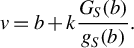 $$ \begin{align} v=b+k\frac{G_S(b)}{g_S(b)}. \end{align} $$
Similarly, for the seller with value $c\leq \overline {b}$
, we have the following condition by (3.6):
$c\leq \overline {b}$
, we have the following condition by (3.6):
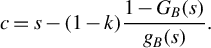 $$ \begin{align} c=s-(1-k)\frac{1-G_B(s)}{g_B(s)}. \end{align} $$
Note that (3.7) and (3.8) only hold for $v\geq \underline {s}$
and
$v\geq \underline {s}$
and $c\leq \overline {b}$
. In such a case, we have
$c\leq \overline {b}$
. In such a case, we have $\Pr (\beta _B(V)\geq \beta _S(C)\mid V=v)>0$
when
$\Pr (\beta _B(V)\geq \beta _S(C)\mid V=v)>0$
when $v>\underline {s}$
and
$v>\underline {s}$
and $\Pr (\beta _B(V)\geq \beta _S(C)\mid C=c)>0$
when
$\Pr (\beta _B(V)\geq \beta _S(C)\mid C=c)>0$
when $c<\overline {b}$
. In other words, given the private values, both the buyer and the seller expect that the trade will occur with a positive probability.Footnote
11
For the buyer with value
$c<\overline {b}$
. In other words, given the private values, both the buyer and the seller expect that the trade will occur with a positive probability.Footnote
11
For the buyer with value $v<\underline {s}$
or the seller with value
$v<\underline {s}$
or the seller with value $c>\overline {b}$
, there will be no transaction under strategy profile
$c>\overline {b}$
, there will be no transaction under strategy profile $(\beta _B,\beta _S)$
. We define the functions
$(\beta _B,\beta _S)$
. We define the functions $\xi (b,G_S)$
and
$\xi (b,G_S)$
and $\eta (s,G_B)$
as the right-hand sides of (3.7) and (3.8), respectively. That is,
$\eta (s,G_B)$
as the right-hand sides of (3.7) and (3.8), respectively. That is,
 $$ \begin{align} \xi(b,G_S) &\equiv b+k\frac{G_S(b)}{g_S(b)}, \quad \underline{s}\leq b\leq \overline{s}, \end{align} $$
 $$ \begin{align} \eta(s,G_B) &\equiv s-(1-k)\frac{1-G_B(s)}{g_B(s)}, \quad \underline{b}\leq s\leq \overline{b}. \end{align} $$
By definition, it is straightforward that $\xi (\underline s,G_S)=\underline s$
and
$\xi (\underline s,G_S)=\underline s$
and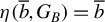 $\eta (\overline b, G_B)=\overline b$
.
$\eta (\overline b, G_B)=\overline b$
.
We define $\mathscr {P}_{\mathscr {A}}$
as the collection of absolutely continuous probability distributions with support
$\mathscr {P}_{\mathscr {A}}$
as the collection of absolutely continuous probability distributions with support $\mathscr {A}$
. Let G denote the joint distribution of
$\mathscr {A}$
. Let G denote the joint distribution of $(B,S)$
. Here, we restrict ourselves to the regular equilibrium strategies which are strictly increasing and (piecewise) differentiable.
$(B,S)$
. Here, we restrict ourselves to the regular equilibrium strategies which are strictly increasing and (piecewise) differentiable.
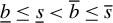
Theorem 1. Under Assumptions C and D, if $G\in \mathscr {P}_{\mathscr {D}}$
is the joint distribution of regular equilibrium bids
$G\in \mathscr {P}_{\mathscr {D}}$
is the joint distribution of regular equilibrium bids $(B,S)$
in a sealed-bid k-double auction with some
$(B,S)$
in a sealed-bid k-double auction with some $(F_V,F_C)$
satisfying Assumptions A and B, then
$(F_V,F_C)$
satisfying Assumptions A and B, then
-
C1. the support
$\mathscr {D}=[\underline {b},\overline {b}] \times [\underline {s},\overline {s}]$
with
$\underline {b} \leq \underline {s} < \overline {b} \leq \overline {s}$
; -
C2.
$G(b,s)=G_B(b)\cdot G_S(s)$
and
$G_B\in \mathscr {P}_{[\underline {b},\overline {b}]}$
,
$G_S\in \mathscr {P}_{[\underline {s},\overline {s}]}$
; -
C3. the function
$\xi (\mkern 2mu\cdot \mkern 2mu,G_S)$
defined in (3.9) is strictly increasing on
$[\underline {s},\overline {b}]$
and its inverse is differentiable on
$[\xi (\underline {s},G_S),\xi (\overline {b},G_S)]$
; -
C4. the function
$\eta (\mkern 2mu\cdot \mkern 2mu,G_B)$
defined in (3.10) is strictly increasing on
$[\underline {s},\overline {b}]$
and its inverse is differentiable on
$[\eta (\underline {s},G_B),\eta (\overline {b},G_B)]$
; -
C5. for any
$b\in [\underline s,\overline b]$
and any
$b'\in [\overline b,\overline s]$
, (3.11)
$$ \begin{align} [\xi(b,G_S)-b']G_S(b')-[\xi(b,G_S)-b]G_S(b) + (1-k)\int_{b}^{b'} G_S(s)\,\mathrm{d} s \leq 0; \end{align} $$
-
C6. for any
$s\in [\underline s,\overline b]$
and any
$s'\in [\underline b,\underline s]$
, (3.12)
$$ \begin{align} [s'-\eta(s,G_B)][1-G_B(s')] &-[s-\eta(s,G_B)][1-G_B(s)] \nonumber \\ & + k\int_{s'}^{s} [1-G_B(b)]\,\mathrm{d} b \leq 0. \end{align} $$














Proof. See Appendix A.4.
Theorem 1 shows that the theoretical model of a k-double auction with bargaining does impose some restrictions on the joint distribution of observed bids.Footnote
12
Together with Theorem 2 which will be shown immediately, these restrictions can be used to establish a formal test of the theory of k-double auction with bargaining. Specifically, condition C1 of Theorem 1 shows that the buyer’s minimum (or maximum) bid is not higher than the seller’s minimum (or maximum) bid, and the intersection between the buyer’s and the seller’s bid supports has a nonempty interior. The latter is mainly due to Assumption B about the supports of private value distributions, which implies that there is always a positive probability of trade in any regular equilibrium. Condition C2 shows that the buyer’s bid is independent of the seller’s. This independence result is intuitive given that the buyer’s value is independent of the seller’s. Conditions C3 and C4 say that the functions $\xi (\mkern 2mu\cdot \mkern 2mu,G_S)$
and
$\xi (\mkern 2mu\cdot \mkern 2mu,G_S)$
and $\eta (\mkern 2mu\cdot \mkern 2mu,G_B)$
, which can be regarded as the inverse bidding strategies, are strictly increasing and differentiable in the interval where there is a positive probability of trade. The strict monotonicity property of the inverse bidding strategies comes from the fact that the equilibrium strategies are strictly increasing. As shown in the proof of Theorem 1, condition C5 is equivalent to a non-profitable deviation for the buyer with a value of
$\eta (\mkern 2mu\cdot \mkern 2mu,G_B)$
, which can be regarded as the inverse bidding strategies, are strictly increasing and differentiable in the interval where there is a positive probability of trade. The strict monotonicity property of the inverse bidding strategies comes from the fact that the equilibrium strategies are strictly increasing. As shown in the proof of Theorem 1, condition C5 is equivalent to a non-profitable deviation for the buyer with a value of $\xi (b,G_S)$
from the equilibrium offer
$\xi (b,G_S)$
from the equilibrium offer $b\in [\underline s,\overline b]$
to an offer
$b\in [\underline s,\overline b]$
to an offer $b'$
higher than the maximum offer
$b'$
higher than the maximum offer $\overline b$
; and condition C6 is equivalent to a no profitable deviation for the seller with a reservation value of
$\overline b$
; and condition C6 is equivalent to a no profitable deviation for the seller with a reservation value of $\eta (s,G_B)$
from the equilibrium ask
$\eta (s,G_B)$
from the equilibrium ask $s\in [\underline s,\overline b]$
to an ask
$s\in [\underline s,\overline b]$
to an ask $s'$
lower than the minimum ask
$s'$
lower than the minimum ask $\underline s$
.
$\underline s$
.
The following theorem establishes our first identification result regarding private value distributions.
Theorem 2. Under Assumptions A–D, $F_V$
and
$F_V$
and $F_C$
are point identified from any given
$F_C$
are point identified from any given $G\in \mathscr {P}_{\mathscr {D}}$
that satisfy C1–C6.
$G\in \mathscr {P}_{\mathscr {D}}$
that satisfy C1–C6.
Proof. See Appendix A.5.
Theorem 2 shows that the private value distributions $F_V$
and
$F_V$
and $F_C$
are point identified from the joint distribution of the observed bids. In particular, if any of the conditions C1–C6 does not hold, then there is no
$F_C$
are point identified from the joint distribution of the observed bids. In particular, if any of the conditions C1–C6 does not hold, then there is no $(F_V,F_C)$
satisfying Assumptions A and B to rationalize the bid distribution G according to Theorem 1. In other words, the identified set is empty when any of those conditions (including conditions C5 and C6) fails. In addition, inverse bidding strategies
$(F_V,F_C)$
satisfying Assumptions A and B to rationalize the bid distribution G according to Theorem 1. In other words, the identified set is empty when any of those conditions (including conditions C5 and C6) fails. In addition, inverse bidding strategies $\xi (\mkern 2mu\cdot \mkern 2mu,G_S)$
and
$\xi (\mkern 2mu\cdot \mkern 2mu,G_S)$
and $\eta (\mkern 2mu\cdot \mkern 2mu,G_B)$
are based only on knowledge of the distribution G. We can therefore avoid solving the linked differential equations (3.5) and (3.6) in our identification.
$\eta (\mkern 2mu\cdot \mkern 2mu,G_B)$
are based only on knowledge of the distribution G. We can therefore avoid solving the linked differential equations (3.5) and (3.6) in our identification.
Conditions C5 and C6 are less intuitive and could be difficult to check in practice. It will be helpful to provide their sufficient conditions that are easy to verify. Our next lemma provides such sufficient conditions.
Lemma 4. Under Assumptions A and B, conditions C3–C6 are implied by:
-
C7. the function
$\xi (\mkern 2mu\cdot \mkern 2mu,G_S)$
defined in (3.9) is strictly increasing on
$[\underline {s},\overline {s}]$
and its inverse is differentiable on
$[\xi (\underline {s},G_S),\xi (\overline {b},G_S)]$
; -
C8. the function
$\eta (\mkern 2mu\cdot \mkern 2mu,G_B)$
defined in (3.10) is strictly increasing on
$[\underline {b},\overline {b}]$
and its inverse is differentiable on
$[\eta (\underline {s},G_B),\eta (\overline {b},G_B)]$
.






Proof. See Appendix A.6.
Conditions C7 and C8 in Lemma 4 are related to conditions C5 and C6 in Theorem 1. The monotonicity of $\xi (\cdot ,G_S)$
in
$\xi (\cdot ,G_S)$
in $[\underline s,\overline s]$
of condition C7 guarantees that the buyer has no profitable deviation from the equilibrium offer to any other offer in
$[\underline s,\overline s]$
of condition C7 guarantees that the buyer has no profitable deviation from the equilibrium offer to any other offer in $[\underline s,\overline s]$
, including any other offer in
$[\underline s,\overline s]$
, including any other offer in $[\overline b,\overline s]$
as stated in condition C5. Similarly, the monotonicity of
$[\overline b,\overline s]$
as stated in condition C5. Similarly, the monotonicity of $\eta (\cdot ,G_B)$
in
$\eta (\cdot ,G_B)$
in $[\underline b,\overline b]$
of condition C8 guarantees that the seller has no profitable deviation from the equilibrium ask to any other ask in
$[\underline b,\overline b]$
of condition C8 guarantees that the seller has no profitable deviation from the equilibrium ask to any other ask in $[\underline b,\overline b]$
, including any other ask in
$[\underline b,\overline b]$
, including any other ask in $[\underline b,\underline s]$
as stated in condition C6. Notice that Assumptions C and D are not needed in Lemma 4.
$[\underline b,\underline s]$
as stated in condition C6. Notice that Assumptions C and D are not needed in Lemma 4.
3.3 Identification with Only Transacted Bids
We now discuss the nonparametric identification of value distributions when only transacted bids are available. To better understand our identification results, we first provide the rationalization results as follows.
Theorem 3. Under Assumptions C and D: If $G_2\in \mathscr {P}_{\mathscr {D'}}$
is the joint distribution of transacted bids under some regular equilibrium in a sealed bid k-double auction with
$G_2\in \mathscr {P}_{\mathscr {D'}}$
is the joint distribution of transacted bids under some regular equilibrium in a sealed bid k-double auction with $(F_V,F_C)$
satisfying Assumptions A and B, then:
$(F_V,F_C)$
satisfying Assumptions A and B, then:
-
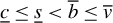
D1. the support
$\mathscr {D'}=\left \{(b,s)\mid \underline {s}\leq s\leq b\leq \overline {b}\right \}$
with
$\underline {s}<\overline {b}$
; -
D2. for any
$\underline {s}\leq s'\leq s\leq b\leq b'\leq \overline {b}$
, the density of
$G_2$
satisfies
$g_2(b,s)\cdot g_2(b',s')=g_2(b,s')\cdot g_2(b',s)$
; -
D3. the function
$\xi (\mkern 2mu\cdot \mkern 2mu,G_{S})$
defined in (3.9) is strictly increasing on
$[\underline {s},\overline {b}]$
and its inverse is differentiable on
$[\xi (\underline {s},G_{S}),\xi (\overline {b},G_{S})]$
; -
D4. the function
$\eta (\mkern 2mu\cdot \mkern 2mu,G_{B})$
defined in (3.10) is strictly increasing on
$[\underline {s},\overline {b}]$
and its inverse is differentiable on
$[\eta (\underline {s},G_{B}),\eta (\overline {b},G_{B})]$
.











Proof. See Appendix A.7.
The rationalization results of Theorem 3 are similar to those of Theorem 1 in the case of using all bids. Specifically, condition D1 says that the support of the distribution of observed (transacted) bids is a triangle in which the buyer’s bid is no less than the seller’s. Condition D2 means that the multiplication of conditional densities evaluated at $(b,s)$
and
$(b,s)$
and $(b',s')$
is the same as the multiplication of conditional densities evaluated at
$(b',s')$
is the same as the multiplication of conditional densities evaluated at $(b,s')$
and
$(b,s')$
and $(b',s)$
as long as these four points are located in the transacted bid area. This condition arises mainly due to the independence of private values. Conditions D3 and D4 state that both the buyer’s and the seller’s inverse bidding strategies are strictly increasing and differentiable on the interval of all possible transacted bid values, namely,
$(b',s)$
as long as these four points are located in the transacted bid area. This condition arises mainly due to the independence of private values. Conditions D3 and D4 state that both the buyer’s and the seller’s inverse bidding strategies are strictly increasing and differentiable on the interval of all possible transacted bid values, namely, $[\underline s, \overline b]$
.
$[\underline s, \overline b]$
.
We next turn to the identification formally. To clarify the idea, we first lay out our identification strategy and then discuss our identification results. Let $G_2$
denote the joint distribution of the transacted bids.Footnote
13
A two-step procedure is employed to accomplish the identification. In the first step, we identify both marginal bid distributions
$G_2$
denote the joint distribution of the transacted bids.Footnote
13
A two-step procedure is employed to accomplish the identification. In the first step, we identify both marginal bid distributions $G_B$
and
$G_B$
and $G_S$
on
$G_S$
on $[\underline {s},\overline {b}]$
from the distribution
$[\underline {s},\overline {b}]$
from the distribution $G_2$
of the transacted bids. For any
$G_2$
of the transacted bids. For any $s\leq \overline {b}$
,
$s\leq \overline {b}$
, $G_S(s) = \Pr (S\leq s | B=\overline {b})$
by the independence between B and S.
$G_S(s) = \Pr (S\leq s | B=\overline {b})$
by the independence between B and S. $\Pr (S\leq s | B=\overline {b})$
is identified from the distribution
$\Pr (S\leq s | B=\overline {b})$
is identified from the distribution $G_2$
of the transacted bids, because the transaction is always successful in this case by
$G_2$
of the transacted bids, because the transaction is always successful in this case by $S\leq s\leq \overline {b} = B$
. The seller’s marginal bid distribution
$S\leq s\leq \overline {b} = B$
. The seller’s marginal bid distribution $G_S(\cdot )$
and its density
$G_S(\cdot )$
and its density $g_S(\cdot )$
are therefore identified on
$g_S(\cdot )$
are therefore identified on $[\underline {s},\overline {b}]$
. Similarly, the marginal bid distribution of the buyer
$[\underline {s},\overline {b}]$
. Similarly, the marginal bid distribution of the buyer $G_B(\cdot )$
and its density
$G_B(\cdot )$
and its density $g_B(\cdot )$
are also identified on
$g_B(\cdot )$
are also identified on $[\underline {s},\overline {b}]$
by
$[\underline {s},\overline {b}]$
by $1-G_B(b) = \Pr (B>b | S = \underline {s})$
for any
$1-G_B(b) = \Pr (B>b | S = \underline {s})$
for any $b\geq \underline {s}$
. In the second step, we recover the corresponding private values for the buyer and the seller by the inverse bidding strategies of (3.9) and (3.10) for the bids on
$b\geq \underline {s}$
. In the second step, we recover the corresponding private values for the buyer and the seller by the inverse bidding strategies of (3.9) and (3.10) for the bids on $[\underline {s},\overline {b}]$
. We formally state the results of this identification strategy as follows.
$[\underline {s},\overline {b}]$
. We formally state the results of this identification strategy as follows.
Theorem 4. Suppose that Assumptions A–D hold. For any joint distribution of transacted bids $G_2\in \mathscr {P}_{\mathscr {D'}}$
satisfying D1–D4, the identified set of value distributions contains all
$G_2\in \mathscr {P}_{\mathscr {D'}}$
satisfying D1–D4, the identified set of value distributions contains all $F_V$
and
$F_V$
and $F_C$
that satisfy
$F_C$
that satisfy
-
E1.
$\underline {c}\leq \underline {s}<\overline {b}\leq \overline {v}$
; -
E2. for all
$(v,c)\in [\underline s,\xi (\overline b,G_{S})]\times [\eta (\underline s,G_{B}),\overline b]$
,Footnote
14
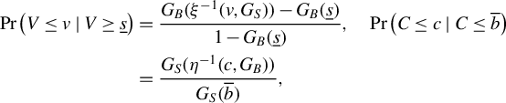
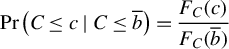
(3.13)where
$$ \begin{align} \Pr\left(V\leq v \mid V\geq \underline s \right) &= \frac{G_B(\xi^{-1}(v,G_{S})) - G_{B}(\underline{s})}{1-G_B(\underline{s})} , \quad \Pr\left(C\leq c \mid C\leq \overline b\right) \nonumber \\ &= \frac{G_S(\eta^{-1}(c,G_{B}))}{G_S(\overline{b})}, \end{align} $$
$\Pr \left (V\leq v\mid V\geq \underline {s}\right )=\dfrac {F_V(v)-F_V(\underline {s})}{1-F_V(\underline {s})}$
, and
$\Pr \left (C\leq c\mid C\leq \overline {b}\right )=\dfrac {F_C(c)}{F_C(\overline {b})}$
.


Proof. See Appendix A.8.
Theorem 4 provides the identified set of model primitives $(F_V,F_C)$
in an implicit way, namely, that the identified set does not have a closed-form expression. In particular, condition E2 provides the main identification restrictions on
$(F_V,F_C)$
in an implicit way, namely, that the identified set does not have a closed-form expression. In particular, condition E2 provides the main identification restrictions on $(F_V,F_C)$
. It provides the (point) identified expressions for
$(F_V,F_C)$
. It provides the (point) identified expressions for $\Pr (V\leq \cdot |V\geq \underline s)$
and
$\Pr (V\leq \cdot |V\geq \underline s)$
and $\Pr (C\leq \cdot | C\leq \overline b)$
that are mappings of
$\Pr (C\leq \cdot | C\leq \overline b)$
that are mappings of $F_V$
and
$F_V$
and $F_C$
.
$F_C$
.
In the parametric case, condition E2 of Theorem 4 is actually useful to obtain the point identification of the parameter of interest under a condition on the Jacobian matrix.Footnote
15
This is summarized by the following theorem. Let $F_V(\cdot )=F_V(\cdot ;\theta _B)$
and
$F_V(\cdot )=F_V(\cdot ;\theta _B)$
and $F_C(\cdot ) = F_C(\cdot ;\theta _S),$
where
$F_C(\cdot ) = F_C(\cdot ;\theta _S),$
where $\theta _B\in \Theta _B \subset \mathbb {R}^{d_B}$
,
$\theta _B\in \Theta _B \subset \mathbb {R}^{d_B}$
, $\theta _S\in \Theta _S \subset \mathbb {R}^{d_S}$
with
$\theta _S\in \Theta _S \subset \mathbb {R}^{d_S}$
with $\Theta _B$
and
$\Theta _B$
and $\Theta _S$
being open sets. Denote
$\Theta _S$
being open sets. Denote ${\mathcal Q}_B(\theta _B;v) \equiv \Pr (V\leq v| V\geq \underline {s})$
,
${\mathcal Q}_B(\theta _B;v) \equiv \Pr (V\leq v| V\geq \underline {s})$
, ${\mathcal Q}_S(\theta _S;c) \equiv \Pr (C\leq c| C\leq \overline {b})$
, and
${\mathcal Q}_S(\theta _S;c) \equiv \Pr (C\leq c| C\leq \overline {b})$
, and $\Theta _B'$
(resp.
$\Theta _B'$
(resp. $\Theta _S'$
) be the collection of
$\Theta _S'$
) be the collection of $\theta _B\in \Theta _B$
(resp.
$\theta _B\in \Theta _B$
(resp. $\theta _S\in \Theta _S$
) such that condition E2 of Theorem 4 holds. In addition, for any
$\theta _S\in \Theta _S$
) such that condition E2 of Theorem 4 holds. In addition, for any $v^m \equiv (v_1,\dots ,v_m)$
and
$v^m \equiv (v_1,\dots ,v_m)$
and $ c^{m'} \equiv (c_1,\dots ,c_{m'})$
, let
$ c^{m'} \equiv (c_1,\dots ,c_{m'})$
, let $J{\mathcal Q}_B(\theta _B;v^m)$
and
$J{\mathcal Q}_B(\theta _B;v^m)$
and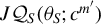 $J{\mathcal Q}_S(\theta _S;c^{m'})$
be the Jacobian matrices of
$J{\mathcal Q}_S(\theta _S;c^{m'})$
be the Jacobian matrices of $({\mathcal Q}_B(\theta _B;v_1),\dots ,{\mathcal Q}_B(\theta _B;v_m))$
(w.r.t.
$({\mathcal Q}_B(\theta _B;v_1),\dots ,{\mathcal Q}_B(\theta _B;v_m))$
(w.r.t. $\theta _B$
) and
$\theta _B$
) and $({\mathcal Q}_S(\theta _S;c_1),\dots ,{\mathcal Q}_S(\theta _S;c_{m'}))$
(w.r.t.
$({\mathcal Q}_S(\theta _S;c_1),\dots ,{\mathcal Q}_S(\theta _S;c_{m'}))$
(w.r.t. $\theta _S$
).
$\theta _S$
).
Theorem 5. Suppose that Assumptions A–D hold. Then $\theta _B$
(resp.
$\theta _B$
(resp. $\theta _S$
) is identified if the following two conditions hold: (i)
$\theta _S$
) is identified if the following two conditions hold: (i) $\Theta _B'$
(resp.
$\Theta _B'$
(resp. $\Theta _S'$
) is convex and (ii) there exists a
$\Theta _S'$
) is convex and (ii) there exists a $v^m$
(resp.
$v^m$
(resp. $c^{m'}$
) and a
$c^{m'}$
) and a $d_B\times d_B$
submatrix
$d_B\times d_B$
submatrix $\overline {JQ}_B$
of
$\overline {JQ}_B$
of $J{\mathcal Q}_B(\theta _B;v^m)$
(resp. a
$J{\mathcal Q}_B(\theta _B;v^m)$
(resp. a $d_S\times d_S$
submatrix
$d_S\times d_S$
submatrix $\overline {JQ}_S$
of
$\overline {JQ}_S$
of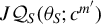 $J{\mathcal Q}_S(\theta _S;c^{m'})$
) such that the determinant of
$J{\mathcal Q}_S(\theta _S;c^{m'})$
) such that the determinant of $\overline {JQ}_B$
(resp.
$\overline {JQ}_B$
(resp. $\overline {JQ}_S$
) is positive and
$\overline {JQ}_S$
) is positive and $\overline {JQ}_B + \overline {JQ}_B'$
(resp.
$\overline {JQ}_B + \overline {JQ}_B'$
(resp. $\overline {JQ}_S + \overline {JQ}_S'$
) is positive semi-definite for all
$\overline {JQ}_S + \overline {JQ}_S'$
) is positive semi-definite for all $\theta _B\in \Theta _B'$
(resp.
$\theta _B\in \Theta _B'$
(resp. $\theta _S\in \Theta _S'$
).
$\theta _S\in \Theta _S'$
).
Proof. See Appendix A.9.
Theorem 5 establishes the identification of $\theta _B$
and
$\theta _B$
and $\theta _S$
under some condition to guarantee the global univalence of the mappings due to Gale and Nikaido (Reference Gale and Nikaido1965). We can show the identification of
$\theta _S$
under some condition to guarantee the global univalence of the mappings due to Gale and Nikaido (Reference Gale and Nikaido1965). We can show the identification of $\theta _B$
and
$\theta _B$
and $\theta _S$
in the neighborhood of their true values under a weaker condition, such as the full column rank of the Jacobian matrix at the true value of parameter (see, e.g., Theorem 6 of Rothenberg, Reference Rothenberg1971).
$\theta _S$
in the neighborhood of their true values under a weaker condition, such as the full column rank of the Jacobian matrix at the true value of parameter (see, e.g., Theorem 6 of Rothenberg, Reference Rothenberg1971).
4 ESTIMATION
Based on the identification strategy, we provide a nonparametric estimation procedure as well as its asymptotic properties when all bids can be observed by the researchers. We will briefly discuss the estimation of the case with only transacted bids in Section S.2.3 of the Supplementary Material.Footnote 16 To present the basic ideas, we further assume that all the observed k-double auctions are homogeneous. Section S.2.1 of the Supplementary Material extends our estimation method to allow auction-specific heterogeneity.
Our estimation procedure extends the two-step estimator proposed by Guerre et al. (Reference Guerre, Perrigne and Vuong2000) for the estimation of sealed-bid first-price auctions: In the first step, a sample of buyers’ and sellers’ “pseudo private values” is constructed by (3.7) and (3.8), where $G_S$
and
$G_S$
and $G_B$
are estimated by their empirical distribution functions, and
$G_B$
are estimated by their empirical distribution functions, and $g_S$
and
$g_S$
and $g_B$
are estimated by their kernel density estimators with boundary and interior bias correction. In the second step, this sample of pseudo private values is used to nonparametrically estimate the densities of buyers’ and sellers’ private values with boundary and interior bias correction. Notice that, due to the regular equilibrium assumption, a bidder’s private value is equal to her bid (in the first step) if the bidder is a buyer offering less than
$g_B$
are estimated by their kernel density estimators with boundary and interior bias correction. In the second step, this sample of pseudo private values is used to nonparametrically estimate the densities of buyers’ and sellers’ private values with boundary and interior bias correction. Notice that, due to the regular equilibrium assumption, a bidder’s private value is equal to her bid (in the first step) if the bidder is a buyer offering less than $\underline s$
or if the bidder is a seller asking more than
$\underline s$
or if the bidder is a seller asking more than $\overline b$
.
$\overline b$
.
It is worth pointing out that both boundary and interior bias correction are implemented in all kernel density estimators of our two-step procedure. This is motivated by the fact that the boundary and interior biases are worse in double auctions than in first-price auctions. Specifically, as pointed out by Guerre et al. (Reference Guerre, Perrigne and Vuong2000), the estimators of bid density and private value density suffer from boundary bias (on the two endpoints of each support) in the two-step estimation of first-price auctions, since these two densities are bounded away from zero on finite supports. This issue carries over to the double auction setup and is made worse by the discontinuity of bid densities in the interior of their supports. The interior discontinuity of bid densities occurs because bidding strategies have interior kinks in regular equilibrium. Consequently, the two-step estimator of private value density with boundary and interior bias correction will have a better performance than the one without any bias correction (e.g., the one with sample trimming instead) in finite samples. This is similar to Hickman and Hubbard (Reference Hickman and Hubbard2014) who corrected the bias on the boundaries (not in the interior) of the bid and value densities, and is confirmed by our Monte Carlo experiments in Section 5 as well.
We apply the boundary-adaptive local polynomial density estimators proposed by Cattaneo et al. (Reference Cattaneo, Jansson and Ma2020) to our double auction setup, and focus on the case of continuously differentiable private value density (and hence twice continuously differentiable bid density by Lemma 3).Footnote 17 The case of smoother private value densities is discussed in Section S.1 of the Supplementary Material.
4.1 Definition of the Estimator
To clarify our idea, we consider n homogeneous k-double auctions. In each auction $i=1,2,\ldots ,n$
, there is one buyer with private value
$i=1,2,\ldots ,n$
, there is one buyer with private value $V_i$
and one seller with private value
$V_i$
and one seller with private value $C_i$
. We observe a sample consisting of all the buyers’ bids
$C_i$
. We observe a sample consisting of all the buyers’ bids $\{B_1,B_2,\ldots ,B_n\}$
and all the sellers’ bids
$\{B_1,B_2,\ldots ,B_n\}$
and all the sellers’ bids $\{S_1,S_2,\ldots ,S_n\}$
. Let
$\{S_1,S_2,\ldots ,S_n\}$
. Let $\hat {\underline b}$
and
$\hat {\underline b}$
and $\hat {\overline b}$
(
$\hat {\overline b}$
( $\hat {\underline s}$
and
$\hat {\underline s}$
and $\hat {\overline s}$
) be the minimum and maximum of the n observed bids of buyers (sellers).
$\hat {\overline s}$
) be the minimum and maximum of the n observed bids of buyers (sellers).
Our estimation proceeds as follows. In the first step, we use the observed sample of all bids to estimate the distribution and density functions of the buyers’ and sellers’ bids by their empirical distribution functions and (boundary and interior) bias-corrected kernel density estimators on the interval of $[\underline s,\overline b]$
, respectively, that is, by
$[\underline s,\overline b]$
, respectively, that is, by
 $$\begin{align*}\hat{G}_B(b) = \frac{1}{n}\sum_{i=1}^n \mathbb{1} (B_i\leq b),\quad \hat{G}_S(s) = \frac{1}{n}\sum_{i=1}^n \mathbb{1}(S_i\leq s), \end{align*}$$
and local quadratic density estimators $\hat {g}_B(b)$
and
$\hat {g}_B(b)$
and $\hat {g}_S(s)$
for all
$\hat {g}_S(s)$
for all $b,s\in [\underline s,\overline b]$
. Specifically, the estimator of the buyer bid density
$b,s\in [\underline s,\overline b]$
. Specifically, the estimator of the buyer bid density $\hat {g}_B$
is defined as followsFootnote
18
:
$\hat {g}_B$
is defined as followsFootnote
18
:
 $$ \begin{align} \hat g_B(b) = \frac{n_B^{+}}{n}\cdot \hat g_B^{+}(b),\quad b\in [\underline s,\overline b], \end{align} $$
where $\hat g_{B}^{+}(\cdot )$
is a local quadratic density estimator using a kernel function of
$\hat g_{B}^{+}(\cdot )$
is a local quadratic density estimator using a kernel function of $K_B$
and a bandwidth of
$K_B$
and a bandwidth of $h_B$
from a subsample
$h_B$
from a subsample $\{B_i: B_i> \hat {\underline s} \}$
(with a size of
$\{B_i: B_i> \hat {\underline s} \}$
(with a size of $n_B^{+}$
). Following Cattaneo et al. (Reference Cattaneo, Jansson and Ma2020), for a given random sample of
$n_B^{+}$
). Following Cattaneo et al. (Reference Cattaneo, Jansson and Ma2020), for a given random sample of $\{Z_1,Z_2,\dots ,Z_m\}$
from a distribution with a density of
$\{Z_1,Z_2,\dots ,Z_m\}$
from a distribution with a density of $g_Z(\cdot )$
on
$g_Z(\cdot )$
on $[\underline z,\overline z]$
, the boundary-adaptive local polynomial density estimator (with a polynomial of order p) is defined as
$[\underline z,\overline z]$
, the boundary-adaptive local polynomial density estimator (with a polynomial of order p) is defined as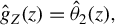 $\hat g_Z(z) = \hat {\theta }_2(z),$
where
$\hat g_Z(z) = \hat {\theta }_2(z),$
where $\hat \theta (z) = \text {argmin}_{\theta \in \mathbb {R}^{p+1}} \sum _{i=1}^m \big [ \hat {G}_Z(Z_i) - \theta _1 - \theta _2\cdot (Z_i-z) - \dots - \theta _{p+1}\cdot (Z_i-z)^p \big ]^2\cdot K\big ((Z_i-z)/h\big )$
with
$\hat \theta (z) = \text {argmin}_{\theta \in \mathbb {R}^{p+1}} \sum _{i=1}^m \big [ \hat {G}_Z(Z_i) - \theta _1 - \theta _2\cdot (Z_i-z) - \dots - \theta _{p+1}\cdot (Z_i-z)^p \big ]^2\cdot K\big ((Z_i-z)/h\big )$
with $\hat G_Z(z) = (1/m)\sum _{i=1}^m \mathbf {1} (Z_i\leq z)$
,
$\hat G_Z(z) = (1/m)\sum _{i=1}^m \mathbf {1} (Z_i\leq z)$
, $K(\cdot )$
being a kernel function, and h being a bandwidth. Similarly, we can define the seller bid density estimator
$K(\cdot )$
being a kernel function, and h being a bandwidth. Similarly, we can define the seller bid density estimator $\hat g_S$
with a cutoff of
$\hat g_S$
with a cutoff of $\hat {\overline b}$
(instead of
$\hat {\overline b}$
(instead of $\hat {\underline s}$
) to split the sample, a kernel function of
$\hat {\underline s}$
) to split the sample, a kernel function of $K_S$
and a bandwidth of
$K_S$
and a bandwidth of $h_S$
, namely,
$h_S$
, namely,
 $$ \begin{align} \hat g_S(s) = \frac{n_S^{-}}{n}\cdot \hat g_S^{-}(s),\quad s\in [\underline s,\overline b], \end{align} $$
where $\hat g_{S}^{-}(\cdot )$
is a local quadratic density estimator from a subsample
$\hat g_{S}^{-}(\cdot )$
is a local quadratic density estimator from a subsample $\{S_i: S_i \leq \hat {\overline b} \}$
(with a size of
$\{S_i: S_i \leq \hat {\overline b} \}$
(with a size of $n_S^{-}$
).
$n_S^{-}$
).
Our bid density estimators $\hat g_B$
and
$\hat g_B$
and $\hat g_S$
, respectively, involve
$\hat g_S$
, respectively, involve $\hat g_B^+$
and
$\hat g_B^+$
and $\hat g_S^-$
which are based on the local quadratic approach (i.e.,
$\hat g_S^-$
which are based on the local quadratic approach (i.e., $p=2$
).Footnote
19
Local quadratic density estimator (with a bandwidth of h) is boundary adaptive and achieves a uniform rate of
$p=2$
).Footnote
19
Local quadratic density estimator (with a bandwidth of h) is boundary adaptive and achieves a uniform rate of $O(h^2)$
while the kernel density estimator (with a bandwidth of h) based on boundary kernel method (e.g., the one discussed in Chapter 1 of Li and Racine, Reference Li and Racine2007) can only achieve a uniform rate of
$O(h^2)$
while the kernel density estimator (with a bandwidth of h) based on boundary kernel method (e.g., the one discussed in Chapter 1 of Li and Racine, Reference Li and Racine2007) can only achieve a uniform rate of $O(h)$
, because the bias of local quadratic method has a rate of
$O(h)$
, because the bias of local quadratic method has a rate of $O(h^2)$
at both the interior and (near) boundary points while the boundary kernel method has a rate of
$O(h^2)$
at both the interior and (near) boundary points while the boundary kernel method has a rate of $O(h)$
at the (near) boundary points (and a rate of
$O(h)$
at the (near) boundary points (and a rate of $O(h^2)$
in the interior).
$O(h^2)$
in the interior).
We then define the buyer’s pseudo private value $\hat V_i$
corresponding to
$\hat V_i$
corresponding to $B_i$
and the seller’s pseudo private value
$B_i$
and the seller’s pseudo private value $\hat C_i$
corresponding to
$\hat C_i$
corresponding to $S_i$
, respectively, as
$S_i$
, respectively, as
 $$ \begin{align} \hat{V}_i &= \begin{cases} B_i + k\dfrac{\hat{G}_S(B_i)}{\hat{g}_S(B_i)} & \text{if } B_i\geq\hat{\underline{s}},\\ B_i & \text{otherwise}, \end{cases}\quad \hat{C}_i = \begin{cases} S_i - (1-k)\dfrac{1-\hat{G}_B(S_i)}{\hat{g}_B(S_i)} & \text{if } S_i\leq\hat{\overline{b}},\\ S_i & \text{otherwise}, \end{cases} \end{align} $$
where $\hat {G}_B(\mkern 2mu\cdot \mkern 2mu),\hat {G}_S(\mkern 2mu\cdot \mkern 2mu),\hat {g}_B(\mkern 2mu\cdot \mkern 2mu)$
, and
$\hat {G}_B(\mkern 2mu\cdot \mkern 2mu),\hat {G}_S(\mkern 2mu\cdot \mkern 2mu),\hat {g}_B(\mkern 2mu\cdot \mkern 2mu)$
, and $\hat {g}_S(\mkern 2mu\cdot \mkern 2mu)$
are the empirical distribution functions and bias-corrected local quadratic density estimators defined earlier.Footnote
20
Note that we have
$\hat {g}_S(\mkern 2mu\cdot \mkern 2mu)$
are the empirical distribution functions and bias-corrected local quadratic density estimators defined earlier.Footnote
20
Note that we have $V_i = B_i$
(resp.
$V_i = B_i$
(resp. $C_i = S_i$
) when
$C_i = S_i$
) when $B_i < \underline {s}$
(resp.
$B_i < \underline {s}$
(resp. $S_i> \overline {b}$
) in regular equilibrium.
$S_i> \overline {b}$
) in regular equilibrium.
In the second step, we use the pseudo private value samples, $\{\hat {V}_1,\ldots ,\hat {V}_n\}$
and
$\{\hat {V}_1,\ldots ,\hat {V}_n\}$
and $\{\hat {C}_1,\ldots ,\hat {C}_n\}$
, to estimate the buyers’ and sellers’ respective value densities. Specifically, the estimator of the buyer value density
$\{\hat {C}_1,\ldots ,\hat {C}_n\}$
, to estimate the buyers’ and sellers’ respective value densities. Specifically, the estimator of the buyer value density $\hat {f}_V$
is obtained by applying the local linear approach (as described previously with
$\hat {f}_V$
is obtained by applying the local linear approach (as described previously with $p=1$
) to the sample of the buyers’ pseudo private values on
$p=1$
) to the sample of the buyers’ pseudo private values on $[\hat {\underline {v}},\hat {\overline {v}}]$
, where
$[\hat {\underline {v}},\hat {\overline {v}}]$
, where $\hat {\underline {v}}$
and
$\hat {\underline {v}}$
and $\hat {\overline {v}}$
are, respectively, the minimum and maximum of the buyers’ pseudo private values, with kernel function
$\hat {\overline {v}}$
are, respectively, the minimum and maximum of the buyers’ pseudo private values, with kernel function $K_V$
and bandwidth
$K_V$
and bandwidth $h_V$
. Similarly, we get the estimator of the sellers’ value density
$h_V$
. Similarly, we get the estimator of the sellers’ value density $\hat {f}_C$
on interval
$\hat {f}_C$
on interval $[\hat {\underline {c}},\hat {\overline {c}}]$
by the sample of the sellers’ pseudo private values with kernel function
$[\hat {\underline {c}},\hat {\overline {c}}]$
by the sample of the sellers’ pseudo private values with kernel function $K_C$
, and bandwidth
$K_C$
, and bandwidth $h_C$
.Footnote
21
$h_C$
.Footnote
21
Remark 1: Our bid density estimators $\hat {g}_B$
and
$\hat {g}_B$
and $\hat {g}_S$
do not include boundaries in their definitions. Our bid density estimator
$\hat {g}_S$
do not include boundaries in their definitions. Our bid density estimator $\hat g_B(\cdot )$
(resp.
$\hat g_B(\cdot )$
(resp. $\hat g_S(\cdot )$
) achieves an asymptotic uniform rate of
$\hat g_S(\cdot )$
) achieves an asymptotic uniform rate of $O_p\big (h_B^2+\sqrt {log(n)/(nh_B)}\big )$
(resp.
$O_p\big (h_B^2+\sqrt {log(n)/(nh_B)}\big )$
(resp. $O_p\big (h_S^2+\sqrt {log(n)/(nh_S)}\big )$
) on the interval of
$O_p\big (h_S^2+\sqrt {log(n)/(nh_S)}\big )$
) on the interval of $[\underline s,\overline b]$
. Note that in our two-step estimation procedure, we only need to estimate
$[\underline s,\overline b]$
. Note that in our two-step estimation procedure, we only need to estimate $g_B(\cdot )$
and
$g_B(\cdot )$
and $g_S(\cdot )$
, respectively, by
$g_S(\cdot )$
, respectively, by $\hat g_B(\cdot )$
and
$\hat g_B(\cdot )$
and $\hat g_S(\cdot )$
in the interval of
$\hat g_S(\cdot )$
in the interval of $[\underline s,\overline b]$
.
$[\underline s,\overline b]$
.
4.2 Asymptotic Properties
The next assumption concerns the process of generating the private values of buyers and sellers $(V_i,C_i), i=1,\dots ,n$
.
$(V_i,C_i), i=1,\dots ,n$
.
Assumption E. $V_i$
,
$V_i$
, $i=1,2,\ldots ,n$
, are independently and identically distributed as
$i=1,2,\ldots ,n$
, are independently and identically distributed as $F_V$
with density
$F_V$
with density $f_V$
;
$f_V$
; $C_i$
,
$C_i$
, $i=1,2,\ldots ,n$
, are independently and identically distributed as
$i=1,2,\ldots ,n$
, are independently and identically distributed as $F_C$
with density
$F_C$
with density $f_C$
.
$f_C$
.
This assumes that the bidders’ private values are independent across auctions.
We turn to the choice of kernels in the following assumption.
Assumption F. $K_B, K_S, K_V$
, and
$K_B, K_S, K_V$
, and $K_C$
are symmetric second-order kernels with support
$K_C$
are symmetric second-order kernels with support $[-1,1]$
and have continuous bounded second-order derivatives.
$[-1,1]$
and have continuous bounded second-order derivatives.
We then give conditions on the choice of bandwidths and other tuning parameters.
Assumption G. The bandwidths $h_B,h_S,h_V,h_C$
are of the form:
$h_B,h_S,h_V,h_C$
are of the form:
 $$\begin{align*} &h_B=\lambda_B \big(\log n /n\big)^{1/5},\quad h_S=\lambda_S\big(\log n/n\big)^{1/5},\quad h_V=\lambda_V\big(\log n/n\big)^{1/5},\quad\\ & h_C=\lambda_C\big(\log n/n\big)^{1/5},\end{align*}$$
where the $\lambda $
’s are positive constants.
$\lambda $
’s are positive constants.
To implement the bias correction technique, we adopt Assumption G to choose all bandwidths of order $(\log n/n)^{1/5}$
.
$(\log n/n)^{1/5}$
.
Our main estimation result establishes the uniform consistency (with rates of convergence) of the two-step estimators of value densities. It is built on the following lemma which shows the uniform consistency (with convergence rates) of (i) the first-step nonparametric estimators of bid densities and (ii) the pseudo private values $\hat {V}_i$
and
$\hat {V}_i$
and $\hat {C}_i$
.
$\hat {C}_i$
.
Lemma 5. Suppose that Assumptions A–G hold, then
(i) $\sup _{b\in [\underline {s},\overline {b}]}|\hat {g}_B(b)-g_B(b)| = O_p\big ((\log n /n)^{2/5}\big ),\quad \sup _{s\in [\underline {s},\overline {b}]} |\hat {g}_S(s)-g_S(s)| = O_p\big ((\log n /n)^{2/5}\big ).$
(ii) $\sup _i|\hat {V}_i-V_i|=O_p\big ((\log n/n)^{2/5}\big ),\quad \sup _i|\hat {C}_i-C_i|=O_p\big ((\log n /n)^{2/5}\big ).$
Proof. See Appendix A.10.
Lemma 5 first shows that, after bias correction, the kernel density estimators of the bid distributions uniformly converge in probability to the true densities at a rate of $(\log n/n)^{2/5}$
on the interval of
$(\log n/n)^{2/5}$
on the interval of $[\underline s,\overline b]$
. It also shows that all pseudo private values converge uniformly in probability to the true private values at the same rate. Without boundary and interior bias correction, the uniform convergence of bid density estimators holds only on an interior closed subset (excluding boundaries) of
$[\underline s,\overline b]$
. It also shows that all pseudo private values converge uniformly in probability to the true private values at the same rate. Without boundary and interior bias correction, the uniform convergence of bid density estimators holds only on an interior closed subset (excluding boundaries) of $[\underline s,\overline b]$
.
$[\underline s,\overline b]$
.
We now give our main result for the estimation section.
Theorem 6. Under Assumptions A–G, for any (fixed) closed inner subsets $\mathscr {C}_V$
of
$\mathscr {C}_V$
of $[\underline {v},\overline {v}]$
and
$[\underline {v},\overline {v}]$
and $\mathscr {C}_C$
of
$\mathscr {C}_C$
of $[\underline {c},\overline {c}]$
,Footnote
22
$[\underline {c},\overline {c}]$
,Footnote
22
 $$\begin{align*}\sup_{v\in\mathscr{C}_V}|\hat{f}_V(v)-f_V(v)|=O_p\big((\log n/n )^{1/5}\big),\quad \sup_{c\in\mathscr{C}_C}|\hat{f}_C(c)-f_C(c)|=O_p\big((\log n /n)^{1/5}\big).\end{align*}$$
Proof. See Appendix A.11.
Remark 2. Theorem 6 shows that our (bias-corrected) two-step estimators of private value densities converge uniformly to their true densities at a rate of $(\log n/n)^{1/5}$
on any closed inner subset of value support. This convergence rate is optimal in first-price auctions (Guerre et al., Reference Guerre, Perrigne and Vuong2000). Without bias correction, the usual two-step estimators of private value densities have the same convergence rate as
$(\log n/n)^{1/5}$
on any closed inner subset of value support. This convergence rate is optimal in first-price auctions (Guerre et al., Reference Guerre, Perrigne and Vuong2000). Without bias correction, the usual two-step estimators of private value densities have the same convergence rate as $(\log n/n)^{1/5}$
only on any close inner subset excluding
$(\log n/n)^{1/5}$
only on any close inner subset excluding $\underline {s}$
(or
$\underline {s}$
(or $\overline {b}$
). Consequently, we expect that, in comparison to the two-step estimator without bias correction, the one with bias correction will have better finite sample performance close to
$\overline {b}$
). Consequently, we expect that, in comparison to the two-step estimator without bias correction, the one with bias correction will have better finite sample performance close to $\underline s$
for the buyers’ value density estimator and close to
$\underline s$
for the buyers’ value density estimator and close to $\overline b$
for the sellers’. This is confirmed by our Monte Carlo experiments in the next section.
$\overline b$
for the sellers’. This is confirmed by our Monte Carlo experiments in the next section.
Remark 3. The uniform convergence rate for estimating value densities is $(\log n / n)^{1/5}$
, which is slower than the
$(\log n / n)^{1/5}$
, which is slower than the $(\log n / n)^{2/5}$
rate for estimating bid densities in Lemma 5. This discrepancy is characteristic of structural auction models (see, e.g., Guerre et al., Reference Guerre, Perrigne and Vuong2000) because private values are not directly observed but must be estimated. If private values were observed, the optimal uniform convergence rate would be
$(\log n / n)^{2/5}$
rate for estimating bid densities in Lemma 5. This discrepancy is characteristic of structural auction models (see, e.g., Guerre et al., Reference Guerre, Perrigne and Vuong2000) because private values are not directly observed but must be estimated. If private values were observed, the optimal uniform convergence rate would be $(\log n/n)^{1/3}$
.
$(\log n/n)^{1/3}$
.
Remark 4. Following Ma, Marmer, and Shneyerov (Reference Ma, Marmer and Shneyerov2019), we propose a percentile bootstrap method to construct pointwise confidence intervals for private value densities using undersmoothed bandwidths. Because the percentile bootstrap avoids explicit estimation of the asymptotic variance, it remains a popular choice for empirical applications. Specifically, we draw M bootstrap samples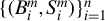 $\{(B_i^m, S_i^m)\}_{i=1}^n$
for
$\{(B_i^m, S_i^m)\}_{i=1}^n$
for $m=1, \dots , M$
independently and with replacement from the original sample of bids
$m=1, \dots , M$
independently and with replacement from the original sample of bids $\{(B_i, S_i)\}_{i=1}^n$
. For each bootstrap sample, we obtain the estimates
$\{(B_i, S_i)\}_{i=1}^n$
. For each bootstrap sample, we obtain the estimates $\hat {f}_V^m(v)$
and
$\hat {f}_V^m(v)$
and $\hat {f}_C^m(c)$
for any
$\hat {f}_C^m(c)$
for any $v \in (\underline {v}, \overline {v})$
and
$v \in (\underline {v}, \overline {v})$
and $c \in (\underline {c}, \overline {c})$
by applying the two-step estimation procedure in Section 4.1. To address asymptotic bias, we employ undersmoothed bandwidths
$c \in (\underline {c}, \overline {c})$
by applying the two-step estimation procedure in Section 4.1. To address asymptotic bias, we employ undersmoothed bandwidths $h_B=h_S=h_V=h_C = \lambda \cdot n^{-\gamma }$
for
$h_B=h_S=h_V=h_C = \lambda \cdot n^{-\gamma }$
for $\lambda> 0$
and
$\lambda> 0$
and $\gamma \in [1/5, 1/3)$
. Let
$\gamma \in [1/5, 1/3)$
. Let $s_{V,\tau }^M$
and
$s_{V,\tau }^M$
and $s_{C,\tau }^M$
denote the
$s_{C,\tau }^M$
denote the $\tau $
-th quantiles of the centered bootstrap distributions
$\tau $
-th quantiles of the centered bootstrap distributions $\{ \hat {f}_V^m(v) - \hat {f}_V(v)\}_{m=1}^M$
and
$\{ \hat {f}_V^m(v) - \hat {f}_V(v)\}_{m=1}^M$
and $\{ \hat {f}_C^m(c) - \hat {f}_C(c)\}_{m=1}^M$
, respectively. Then, the percentile bootstrap confidence intervals with nominal coverage
$\{ \hat {f}_C^m(c) - \hat {f}_C(c)\}_{m=1}^M$
, respectively. Then, the percentile bootstrap confidence intervals with nominal coverage $1-\alpha $
are
$1-\alpha $
are
 $$ \begin{align*}\text{CI}_{1-\alpha}^{V,M}(v) = [\hat{f}_V(v) + s_{V,\alpha/2}^M, \hat{f}_V(v) + s_{V,1-\alpha/2}^M]\end{align*} $$
and
 $$ \begin{align*}\text{CI}_{1-\alpha}^{C,M}(c) = [\hat{f}_C(c) + s_{C,\alpha/2}^M, \hat{f}_C(c) + s_{C,1-\alpha/2}^M].\end{align*} $$
Section 5 examines the finite-sample performance of these intervals (see Table 1 and accompanying discussion).
Simulated coverage rates of pointwise confidence intervals $\text {CI}_{1-\alpha }^{V,M}(v)$
and
$\text {CI}_{1-\alpha }^{V,M}(v)$
and $\text {CI}_{1-\alpha }^{C,M}(c)$
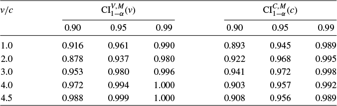
With smoother value densities, the uniform convergence rate of the two-step value density estimators can be improved. This extension is briefly discussed in Section S.1 of the Supplementary Material.
5 MONTE CARLO EXPERIMENTS
To study the finite sample performance of our two-step estimation procedure, we performed Monte Carlo experiments. We consider an empirically relevant design in which the bid distributions are specified as log-normal (up to some truncation). Log-normal bid distributions have been used extensively in the empirical auction literature (see, e.g., Laffont, Ossard, and Vuong, Reference Laffont, Ossard and Vuong1995; Hong and Shum, Reference Hong and Shum2002). Specifically, let $[\underline v,\overline v] = [\underline c,\overline c] = [0.5,5]$
so that
$[\underline v,\overline v] = [\underline c,\overline c] = [0.5,5]$
so that $\underline b=0.5$
,
$\underline b=0.5$
, $\underline s = 1$
,
$\underline s = 1$
, $\overline b = 4.5$
, and
$\overline b = 4.5$
, and ${\overline s =5}$
. We assume that the buyers’ and sellers’ bids are distributed as a log-normal with mean 0 and standard deviation 1 up to some truncation. The truncation is made in three regions:
${\overline s =5}$
. We assume that the buyers’ and sellers’ bids are distributed as a log-normal with mean 0 and standard deviation 1 up to some truncation. The truncation is made in three regions: $[0.5,1]$
,
$[0.5,1]$
, $[1,4.5]$
, and
$[1,4.5]$
, and $[4.5,5]$
. It introduces a probability of
$[4.5,5]$
. It introduces a probability of $1/2$
in both
$1/2$
in both $[0.5,1]$
and
$[0.5,1]$
and $[1,4.5]$
for buyer bids and in both
$[1,4.5]$
for buyer bids and in both $[1,4.5]$
and
$[1,4.5]$
and $[4.5,5]$
for seller bids. Given such (truncated) log-normal bid distributions, we can recover the inverse bidding strategies according to (3.9) and (3.10), and further recover the value distributions. In addition, we give equal pricing weights to both buyers and sellers as
$[4.5,5]$
for seller bids. Given such (truncated) log-normal bid distributions, we can recover the inverse bidding strategies according to (3.9) and (3.10), and further recover the value distributions. In addition, we give equal pricing weights to both buyers and sellers as $k = 1/2$
.
$k = 1/2$
.
Our Monte Carlo experiment consists of 1,000 replications. In each replication, we first randomly generate n buyers’ and n sellers’ bids from the truncated log-normal distributions. Next, we apply our bias-corrected two-step estimation procedure to the generated sample of bids for each replication. In the first step, we estimate the distribution functions and densities of buyers’ and sellers’ bids using the empirical distribution functions and local polynomial density estimators, respectively. We then use (4.3) to obtain the pseudo private values of buyers and sellers. In the second step, we used the sample of buyers’ and sellers’ pseudo private values to estimate buyers’ and sellers’ value densities by their local polynomial density estimators.
We choose a triangular kernel in our local polynomial density estimators and use the rule of thumb to determine the bandwidth as $h = 1.06 \cdot \hat {\sigma } \cdot n^{-1/5}$
, where
$h = 1.06 \cdot \hat {\sigma } \cdot n^{-1/5}$
, where $\hat \sigma $
is the standard error of the given sample. Other kernels can also be used.
$\hat \sigma $
is the standard error of the given sample. Other kernels can also be used.
Our Monte Carlo results for estimation are summarized in Figure 1. It shows the two-step estimates of the buyer value density $f_V(\cdot )$
with and without bias correction under the sample sizes of
$f_V(\cdot )$
with and without bias correction under the sample sizes of $n=200$
and
$n=200$
and $n=1,000$
. Similar results can be obtained for estimating the seller value density
$n=1,000$
. Similar results can be obtained for estimating the seller value density $f_C(\cdot )$
. The true value density is displayed in solid line. For each value of
$f_C(\cdot )$
. The true value density is displayed in solid line. For each value of $v\in [0.5,5]$
, we plot the mean of the estimates with a dashed line and the 5th and 95th percentiles with dotted lines. The latter gives the (pointwise) 90% confidence interval for
$v\in [0.5,5]$
, we plot the mean of the estimates with a dashed line and the 5th and 95th percentiles with dotted lines. The latter gives the (pointwise) 90% confidence interval for $f_V(v)$
. Figure 1 shows that our bias-corrected two-step density estimates behave well. First, the true curves fall within their corresponding confidence bands. Second, the mean of the estimates for each density closely matches the true curve. Third, as the sample size increases, both the bias and variance of the estimates decrease. Figure 1 also shows that bias correction plays an important role in estimating the value densities in double auctions with bargaining. In particular, the standard kernel density estimator (without bias correction) has a large bias not only at the boundaries but also in an interior area. When the sample size n increases, this bias will not decrease, although the variance will decrease. The appearance of bias in the interior shows that bias correction is necessary to estimate value densities in double auctions with bargaining.
$f_V(v)$
. Figure 1 shows that our bias-corrected two-step density estimates behave well. First, the true curves fall within their corresponding confidence bands. Second, the mean of the estimates for each density closely matches the true curve. Third, as the sample size increases, both the bias and variance of the estimates decrease. Figure 1 also shows that bias correction plays an important role in estimating the value densities in double auctions with bargaining. In particular, the standard kernel density estimator (without bias correction) has a large bias not only at the boundaries but also in an interior area. When the sample size n increases, this bias will not decrease, although the variance will decrease. The appearance of bias in the interior shows that bias correction is necessary to estimate value densities in double auctions with bargaining.
True and estimated densities of private values.
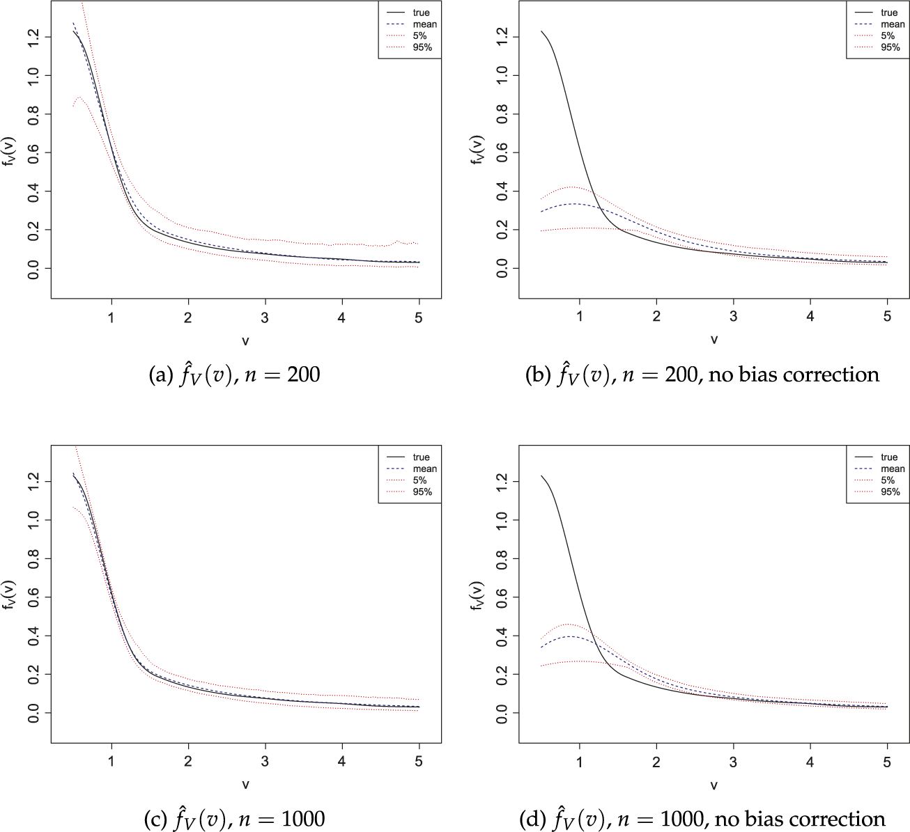
Our simulation results for the pointwise confidence intervals are summarized in Table 1. This table reports the simulated coverage rates of $\text {CI}_{1-\alpha }^{V,M}(v)$
and
$\text {CI}_{1-\alpha }^{V,M}(v)$
and $\text {CI}_{1-\alpha }^{C,M}(c)$
(as defined in Remark 4) using
$\text {CI}_{1-\alpha }^{C,M}(c)$
(as defined in Remark 4) using $M=1,000$
bootstrap replications and a sample size of
$M=1,000$
bootstrap replications and a sample size of $n=1,000$
. As shown in Table 1, the intervals perform well in finite samples. Specifically, the simulated coverage rates for both intervals meet or exceed the nominal levels for most values of v and c. In the few instances where coverage falls slightly below the nominal level—for example, at
$n=1,000$
. As shown in Table 1, the intervals perform well in finite samples. Specifically, the simulated coverage rates for both intervals meet or exceed the nominal levels for most values of v and c. In the few instances where coverage falls slightly below the nominal level—for example, at $v = 2$
or
$v = 2$
or $c=1$
—the distortions remain minimal.
$c=1$
—the distortions remain minimal.
6 CONCLUSION
This article studies nonparametric identification and estimation of double auction with bargaining. It first gives all the restrictions of the theoretical model on observed bid distributions, as well as the sharp identified set of unobserved private value distributions when only transacted bids are used. The latter identified set collapses to singleton when the non-transacted bids are also used. We then propose a (boundary and interior) bias-corrected two-step estimators of the buyer’s and the seller’s value densities. The estimators are shown to achieve the optimal convergence rate. Our Monte Carlo experiments demonstrate the significance of the bias correction (especially the bias correction in the interior of the support) in the two-step estimation of the value densities.
We focus on the identification and estimation of double auction with bargaining. It is interesting to design some nonparametric testing procedures in the context of double auctions, similar to those testing procedures proposed in one-sided auctions (see, e.g., Liu and Luo, Reference Liu and Luo2017; Liu and Vuong, Reference Liu and Vuong2021; Jun and Zincenko, Reference Jun and Zincenko2022).
APPENDIX
Appendix A collects the proofs of theorems and lemmas in the text. The Supplementary Material is also available for additional results and their proofs.
A PROOFS OF THEOREMS AND LEMMAS IN THE TEXT
A.1 Proof of Lemma 1
First, we prove that $v>\underline {s}$
implies
$v>\underline {s}$
implies $\beta _B(v)\leq v$
.
$\beta _B(v)\leq v$
.
When $k=0$
, that is, the transaction price is completely determined by the seller’s bid, a buyer with private value
$k=0$
, that is, the transaction price is completely determined by the seller’s bid, a buyer with private value $v\geq \underline {s}$
will get
$v\geq \underline {s}$
will get
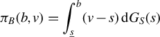 $$\begin{align*}\pi_B(b,v)=\int_{\underline{s}}^b (v-s)\,\mathrm{d} G_S(s)\end{align*}$$
from bidding b. Note that the integrand, $v-s$
, is strictly decreasing in s, thus
$v-s$
, is strictly decreasing in s, thus
 $$ \begin{align} \int_{\underline{s}}^b (v-s)\,\mathrm{d} G_S(s)\leq \int_{\underline{s}}^{+\infty}\max\{v-s,0\} \,\mathrm{d} G_S(s). \end{align} $$
Since $v>\underline {s}$
, the equality in (A.1) holds if
$v>\underline {s}$
, the equality in (A.1) holds if $b=v$
, and the equality holds for all
$b=v$
, and the equality holds for all $G_S$
only if
$G_S$
only if $b=v$
. This implies that, when
$b=v$
. This implies that, when $k=0$
, the truthful strategy
$k=0$
, the truthful strategy $\beta _B(v)=v$
is the unique (weakly) dominant strategy for the buyer.
$\beta _B(v)=v$
is the unique (weakly) dominant strategy for the buyer.
When $k\in (0,1]$
, we shall show that it is better for the buyer with value
$k\in (0,1]$
, we shall show that it is better for the buyer with value $v>\underline {s}$
to bid her value v than any bid
$v>\underline {s}$
to bid her value v than any bid $b>v$
. Since
$b>v$
. Since $\underline {s}$
is the lower bound of the support of
$\underline {s}$
is the lower bound of the support of $G_S$
,
$G_S$
, $G_S(\underline {s})=0$
and
$G_S(\underline {s})=0$
and $G_S(v)>0$
, then
$G_S(v)>0$
, then
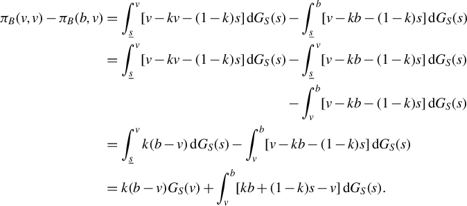 $$ \begin{align*} \pi_B(v,v)-\pi_B(b,v) &= \int_{\underline{s}}^v [v-kv-(1-k)s]\,\mathrm{d} G_S(s)-\int_{\underline{s}}^b [v-kb-(1-k)s]\,\mathrm{d} G_S(s)\\ &= \begin{aligned}[t] \int_{\underline{s}}^v [v-kv-(1-k)s]\,\mathrm{d} G_S(s)-\int_{\underline{s}}^v [v-kb-(1-k)s]\,\mathrm{d} G_S(s)\\ -\int_v^b [v-kb-(1-k)s]\,\mathrm{d} G_S(s) \end{aligned}\\ &= \int_{\underline{s}}^v k(b-v)\,\mathrm{d} G_S(s)-\int_v^b [v-kb-(1-k)s]\,\mathrm{d} G_S(s)\\ &= k(b-v)G_S(v)+\int_v^b [kb+(1-k)s-v]\,\mathrm{d} G_S(s). \end{align*} $$
Since $b>v$
and
$b>v$
and $G_S(v)>0$
, the first term is positive and the second term
$G_S(v)>0$
, the first term is positive and the second term
 $$\begin{align*}\int_v^b [kb+(1-k)s-v]\,\mathrm{d} G_S(s) &\geq \int_v^b [kb+(1-k)v-v]\,\mathrm{d} G_S(s) \\ &=k(b-v)[G_S(b)-G_S(v)]\geq 0. \end{align*}$$
This completes the proof of $\beta _B(v)\leq v$
.
$\beta _B(v)\leq v$
.
To see that $\beta _B(v)<v$
for
$\beta _B(v)<v$
for $v>\underline {s}$
if
$v>\underline {s}$
if $k>0$
, note that by (2.1),
$k>0$
, note that by (2.1),
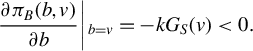 $$ \begin{align*} \left.\frac{\partial\pi_B(b,v)}{\partial b}\right|{}_{b=v}=-kG_S(v)<0. \end{align*} $$
It implies that there exists $\Delta>0$
small enough such that
$\Delta>0$
small enough such that $\pi _B(v-\Delta ,v)>\pi _B(v,v)$
, therefore, bidding the true value for the buyer with private value v is no longer optimal, that is,
$\pi _B(v-\Delta ,v)>\pi _B(v,v)$
, therefore, bidding the true value for the buyer with private value v is no longer optimal, that is, ${\beta _B(v)\neq v}$
. Since we have already shown that
${\beta _B(v)\neq v}$
. Since we have already shown that $\beta _B(v)\leq v$
, the desired result follows.
$\beta _B(v)\leq v$
, the desired result follows.
In an analogous way, the second conclusion can be proved by showing that the truthful bidding strategy is dominant when $k=1$
and is dominated by some
$k=1$
and is dominated by some $\tilde \beta _S(c)>c$
when
$\tilde \beta _S(c)>c$
when $k\in [0,1)$
and
$k\in [0,1)$
and $c<\overline {b}$
.
$c<\overline {b}$
.
A.2 Proof of Lemma 2
First, note that when $k\in (0,1]$
, we can rewrite (3.1) and (3.3) together as
$k\in (0,1]$
, we can rewrite (3.1) and (3.3) together as
 $$ \begin{align} \Psi_k(p)=\int_{\underline{s}}^p \int_s^{\min\left(\frac{p-(1-k)s}{k},\overline{b}\right)} g_2(b,s)\,\mathrm{d} b\,\mathrm{d} s. \end{align} $$
Keep $p\in (\underline {s},\overline {b})$
fixed and define a function
$p\in (\underline {s},\overline {b})$
fixed and define a function $\varphi $
as the inner integral in (A.2), that is,
$\varphi $
as the inner integral in (A.2), that is,
 $$ \begin{align} \varphi(k,s)=\int_s^{\min\left(\frac{p-(1-k)s}{k},\overline{b}\right)} g_2(b,s)\,\mathrm{d} b,\quad k\in(0,1],\ s\in[\underline{s},p]. \end{align} $$
Since $g_2(b,s)$
is integrable,
$g_2(b,s)$
is integrable, $\varphi $
is continuous in the upper limit of the integral. And since the upper limit,
$\varphi $
is continuous in the upper limit of the integral. And since the upper limit,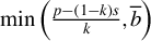 $\min \left (\frac {p-(1-k)s}{k},\overline {b}\right )$
, is continuous in k,
$\min \left (\frac {p-(1-k)s}{k},\overline {b}\right )$
, is continuous in k, $\varphi $
is continuous in k. Note that
$\varphi $
is continuous in k. Note that $g_2(b,s)>0$
because the integration interval is in support of G, and note that
$g_2(b,s)>0$
because the integration interval is in support of G, and note that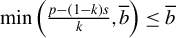 $\min \left (\frac {p-(1-k)s}{k},\overline {b}\right )\le \overline {b}$
, thus for any
$\min \left (\frac {p-(1-k)s}{k},\overline {b}\right )\le \overline {b}$
, thus for any $k\in (0,1]$
,
$k\in (0,1]$
,
 $$\begin{align*}0\le \varphi(k,s)\le \int_s^{\overline{b}} g_2(b,s)\,\mathrm{d} b\equiv \bar{\varphi}(s),\quad \forall\,s\in[\underline{s},p]. \end{align*}$$
Therefore, for any $k\in (0,1]$
, for any sequence
$k\in (0,1]$
, for any sequence $\{k_n\}$
in
$\{k_n\}$
in $(0,1]$
such that
$(0,1]$
such that $k_n\to k$
as
$k_n\to k$
as $n\to \infty $
, by continuity of
$n\to \infty $
, by continuity of $\varphi $
in k, we have
$\varphi $
in k, we have $\tilde {\varphi }_n(s)\equiv \varphi (k_n,s)$
converges pointwise to
$\tilde {\varphi }_n(s)\equiv \varphi (k_n,s)$
converges pointwise to $\tilde {\varphi }(s)\equiv \varphi (k,s)$
in
$\tilde {\varphi }(s)\equiv \varphi (k,s)$
in $[\underline {s},p]$
. Since
$[\underline {s},p]$
. Since $\bar {\varphi }(s)$
is integrable, by the dominated convergence theorem, as
$\bar {\varphi }(s)$
is integrable, by the dominated convergence theorem, as $n\to \infty $
,
$n\to \infty $
,
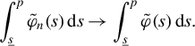 $$\begin{align*}\int_{\underline{s}}^p \tilde{\varphi}_n(s)\,\mathrm{d} s\to\int_{\underline{s}}^p \tilde{\varphi}(s)\,\mathrm{d} s. \end{align*}$$
This implies $\Psi _{k_n}(p)\to \Psi _k(p)$
.
$\Psi _{k_n}(p)\to \Psi _k(p)$
.
To see the (right) continuity at $k=0$
, we just need to rewrite (3.1) and (3.2) as
$k=0$
, we just need to rewrite (3.1) and (3.2) as
 $$\begin{align*}\Psi_k(p) = 1-\int_p^{\overline{b}} \int_{\frac{p-kb}{1-k}}^b g_2(b,s)\,\mathrm{d} s\,\mathrm{d} b,\quad 0\le k<\frac{p-\underline{s}}{\overline{b}-\underline{s}} \end{align*}$$
and define
 $$\begin{align*}\psi(k,b) = -\int_{\frac{p-kb}{1-k}}^b g(b,s)\,\mathrm{d} s,\quad k\in\left[0,\frac{p-\underline{s}}{\overline{b}-\underline{s}}\right),\ b\in[p,\overline{b}].\end{align*}$$
Then applying analogous argument, we have that $\psi $
is continuous in k so that for the sequence
$\psi $
is continuous in k so that for the sequence $\{k_n\}$
in
$\{k_n\}$
in $\left [0,\frac {p-\underline {s}}{\overline {b}-\underline {s}}\right )$
such that
$\left [0,\frac {p-\underline {s}}{\overline {b}-\underline {s}}\right )$
such that $k_n\to 0$
, the sequence
$k_n\to 0$
, the sequence $\{\tilde {\psi }_n(b)\equiv \psi (k_n,b)\}$
converges pointwise to
$\{\tilde {\psi }_n(b)\equiv \psi (k_n,b)\}$
converges pointwise to $\tilde {\psi }(b)\equiv \psi (0,b)$
. Since
$\tilde {\psi }(b)\equiv \psi (0,b)$
. Since $\{\tilde {\psi }_n(b)\}$
is dominated by
$\{\tilde {\psi }_n(b)\}$
is dominated by $\bar {\psi }(b)\equiv \int _{\underline {s}}^b g(b,s)\,\mathrm {d} s$
, we can finally obtain
$\bar {\psi }(b)\equiv \int _{\underline {s}}^b g(b,s)\,\mathrm {d} s$
, we can finally obtain $\Psi _{k_n}(p)\to \Psi _0(p)$
.
$\Psi _{k_n}(p)\to \Psi _0(p)$
.
It remains to show the monotonicity of $\Psi _k(p)$
in k. Suppose
$\Psi _k(p)$
in k. Suppose $0\le k_1<k_2\le 1$
, then by (3.1)–(3.3):
$0\le k_1<k_2\le 1$
, then by (3.1)–(3.3):
-
(i) If
$k_2<\frac {p-\underline {s}}{\overline {b}-\underline {s}}$
, then due to
$$\begin{align*}\Psi_{k_1}(p)-\Psi_{k_2}(p) = \int_p^{\overline{b}}\int_{b-\frac{b-p}{1-k_2}}^{b-\frac{b-p}{1-k_1}} g_2(b,s)\,\mathrm{d} s\,\mathrm{d} b>0\end{align*}$$
$\frac {b-p}{1-k_2}>\frac {b-p}{1-k_1}$
.
-
(ii) If
$k_1\ge \frac {p-\underline {s}}{\overline {b}-\underline {s}}$
, then due to
$$\begin{align*}\Psi_{k_1}(p)-\Psi_{k_2}(p) = \int_{\underline{s}}^p \int_{s+\frac{p-s}{k_2}}^{s+\frac{p-s}{k_1}} g_2(b,s)\,\mathrm{d} b\,\mathrm{d} s>0\end{align*}$$
$\frac {p-s}{k_2}<\frac {p-s}{k_1}$
.
-
(iii) If
$k_1<\frac {p-\underline {s}}{\overline {b}-\underline {s}}\le k_2$
, then where the first term is nonnegative and the second is positive.
$$\begin{align*}\Psi_{k_1}(p)-\Psi_{k_2}(p) &=\int_{\underline{s}}^p \int_{s+\frac{p-s}{k_2}}^{s+\frac{(p-s)(\overline{b} -\underline{s})}{p-\underline{s}}} g_2(b,s)\,\mathrm{d} b\,\mathrm{d} s \\ &\quad + \int_p^{\overline{b}} \int_{b-\frac{(b-p)(\overline{b}-\underline{s})}{\overline{b}-p}}^{b-\frac{b-p}{1-k_1}} g_2(b,s)\,\mathrm{d} s \,\mathrm{d} b>0,\end{align*}$$






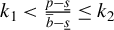
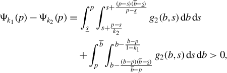
A.3 Proof of Lemma 3
First, we will establish the following two properties in bidding strategies: (M1) under Assumption A, any regular equilibrium strategies $\beta _B$
and
$\beta _B$
and $\beta _S$
are twice continuously differentiable in
$\beta _S$
are twice continuously differentiable in $[\underline {s},\overline {v}]$
and
$[\underline {s},\overline {v}]$
and $[\underline {c},\overline {b}]$
, respectively and (M2) for any
$[\underline {c},\overline {b}]$
, respectively and (M2) for any $v\in [\underline {s},\overline {v}]$
and any
$v\in [\underline {s},\overline {v}]$
and any $c\in [\underline {c},\overline {b}]$
,
$c\in [\underline {c},\overline {b}]$
, $\beta ^{\prime }_B(v)\geq \epsilon _B>0$
and
$\beta ^{\prime }_B(v)\geq \epsilon _B>0$
and $\beta ^{\prime }_S(c)\geq \epsilon _S>0$
. To show (M1), we need to rewrite (3.5) and (3.6) as follows:
$\beta ^{\prime }_S(c)\geq \epsilon _S>0$
. To show (M1), we need to rewrite (3.5) and (3.6) as follows:
 $$ \begin{align} \beta_S'(c) &= \frac{f_C(c)\big[\beta_B^{-1}(\beta_S(c))-\beta_S(c)\big]}{k\cdot F_C(c)}, \end{align} $$
 $$ \begin{align} \beta_B'(v) &= \frac{f_V(v)\big[\beta_B(v)-\beta_S^{-1}(\beta_B(v))\big]}{(1-k)\cdot [1-F_V(v)]}. \end{align} $$
By definition, any pair of regular equilibrium strategies $\beta _B$
and
$\beta _B$
and $\beta _S$
is continuously differentiable in
$\beta _S$
is continuously differentiable in $[\underline s,\overline v]$
and
$[\underline s,\overline v]$
and $[\underline c, \overline b]$
, respectively (see Assumption C). Consequently, under Assumption A, (A.4) and (A.5) imply that
$[\underline c, \overline b]$
, respectively (see Assumption C). Consequently, under Assumption A, (A.4) and (A.5) imply that $\beta _S'(\mkern 2mu\cdot \mkern 2mu)$
and
$\beta _S'(\mkern 2mu\cdot \mkern 2mu)$
and $\beta _B'(\mkern 2mu\cdot \mkern 2mu)$
are continuously differentiable in
$\beta _B'(\mkern 2mu\cdot \mkern 2mu)$
are continuously differentiable in $[\underline c,\overline b]$
and
$[\underline c,\overline b]$
and $[\underline s,\overline v]$
, respectively. This further implies that
$[\underline s,\overline v]$
, respectively. This further implies that $\beta _S$
and
$\beta _S$
and $\beta _B$
are twice continuously differentiable in
$\beta _B$
are twice continuously differentiable in $[\underline c,\overline b]$
and
$[\underline c,\overline b]$
and $[\underline s,\overline v]$
. This completes the proof of (M1).
$[\underline s,\overline v]$
. This completes the proof of (M1).
Now, we establish (M2). By definition of regular equilibrium, the seller and buyer bidding strategies are continuously differentiable with positive derivative on $[\underline c,\overline b]$
and
$[\underline c,\overline b]$
and $[\underline s,\overline v]$
, respectively (see condition A2 of Assumption C), that is,
$[\underline s,\overline v]$
, respectively (see condition A2 of Assumption C), that is, $\beta _S'(\mkern 2mu\cdot \mkern 2mu)$
and
$\beta _S'(\mkern 2mu\cdot \mkern 2mu)$
and $\beta _B'(\mkern 2mu\cdot \mkern 2mu)$
are continuous and positive on
$\beta _B'(\mkern 2mu\cdot \mkern 2mu)$
are continuous and positive on $[\underline c,\overline b]$
and
$[\underline c,\overline b]$
and $[\underline s,\overline v]$
. By the extreme value theorem,
$[\underline s,\overline v]$
. By the extreme value theorem, $\beta _S'(\mkern 2mu\cdot \mkern 2mu)$
and
$\beta _S'(\mkern 2mu\cdot \mkern 2mu)$
and $\beta _B'(\mkern 2mu\cdot \mkern 2mu)$
have positive minimum and maximum in
$\beta _B'(\mkern 2mu\cdot \mkern 2mu)$
have positive minimum and maximum in $[\underline c,\overline b]$
and
$[\underline c,\overline b]$
and $[\underline s,\overline v]$
, respectively. Therefore, the conclusion of (M2) follows.
$[\underline s,\overline v]$
, respectively. Therefore, the conclusion of (M2) follows.
By (A.8) and (A.9), conditions (M1) and (M2) imply that both $\xi (\mkern 2mu\cdot \mkern 2mu,G_S)$
and
$\xi (\mkern 2mu\cdot \mkern 2mu,G_S)$
and $\eta (\mkern 2mu\cdot \mkern 2mu,G_B)$
are twice continuously differentiable on
$\eta (\mkern 2mu\cdot \mkern 2mu,G_B)$
are twice continuously differentiable on $[\underline {s},\overline {b}]$
. Note that
$[\underline {s},\overline {b}]$
. Note that
 $$\begin{align*}g_B(b)=\frac{f_V(\beta_B^{-1}(b))}{\beta^{\prime}_B(\beta_B^{-1}(b))},\quad g_S(s)=\frac{f_C(\beta_S^{-1}(s))}{\beta^{\prime}_S(\beta_S^{-1}(s))}. \end{align*}$$
In addition, $f_V$
and
$f_V$
and $f_C$
are bounded away from 0 by Assumption A, and
$f_C$
are bounded away from 0 by Assumption A, and $\beta ^{\prime }_B$
and
$\beta ^{\prime }_B$
and $\beta ^{\prime }_S$
are bounded away from 0 by (M2). The conclusion of part (i) then follows. Lastly, to prove part (ii), notice that (3.7) and (3.8) yield the following:
$\beta ^{\prime }_S$
are bounded away from 0 by (M2). The conclusion of part (i) then follows. Lastly, to prove part (ii), notice that (3.7) and (3.8) yield the following:
 $$\begin{align*}g_S(s)=k\frac{G_S(s)}{\xi(s,G_S)-s},\quad g_B(b)=(1-k)\frac{1-G_B(b)}{b-\eta(b,G_B)}. \end{align*}$$
Since every term on the right-hand side is twice continuously differentiable, the desired conclusion follows.
A.4 Proof of Theorem 1
Let $\beta _B(\mkern 2mu\cdot \mkern 2mu)$
and
$\beta _B(\mkern 2mu\cdot \mkern 2mu)$
and $\beta _S(\mkern 2mu\cdot \mkern 2mu)$
be the respective regular equilibrium bidding strategies of the buyer and the seller that induce the bid distribution G.
$\beta _S(\mkern 2mu\cdot \mkern 2mu)$
be the respective regular equilibrium bidding strategies of the buyer and the seller that induce the bid distribution G.
By Condition A1 of Assumption C, the strictly increasing and continuous bidding strategies imply that the support of bid distribution is a rectangular region, namely, $[\underline {b},\overline {b}]\times [\underline {s},\overline {s}]$
with
$[\underline {b},\overline {b}]\times [\underline {s},\overline {s}]$
with $\underline {b}=\beta _B(\underline {v})$
,
$\underline {b}=\beta _B(\underline {v})$
, $\overline {b}=\beta _B(\overline {v})$
,
$\overline {b}=\beta _B(\overline {v})$
, $\underline {s}=\beta _S(\underline {c}),$
and
$\underline {s}=\beta _S(\underline {c}),$
and $\overline {s}=\beta _S(\overline {c})$
. To show that
$\overline {s}=\beta _S(\overline {c})$
. To show that $\overline {b}\leq \overline {s}$
and
$\overline {b}\leq \overline {s}$
and $\underline {b}\leq \underline {s}$
, first suppose that
$\underline {b}\leq \underline {s}$
, first suppose that $\overline {b}>\overline {s}$
, then any buyer bidding
$\overline {b}>\overline {s}$
, then any buyer bidding $b>\overline {s}$
will be strictly inferior to bidding only
$b>\overline {s}$
will be strictly inferior to bidding only $\overline {s}$
. Because this does not make the buyer lose any trades, but the expected profit on each trade will increase by lowering the transaction price. This deviation is contradicted by the assumption that
$\overline {s}$
. Because this does not make the buyer lose any trades, but the expected profit on each trade will increase by lowering the transaction price. This deviation is contradicted by the assumption that $(\beta _B,\beta _S)$
is an equilibrium. Applying a similar argument to the seller’s bidding
$(\beta _B,\beta _S)$
is an equilibrium. Applying a similar argument to the seller’s bidding $s<\underline {b}$
, we can prove the second conclusion
$s<\underline {b}$
, we can prove the second conclusion $\underline {s}\geq \underline {b}$
. Then we show that
$\underline {s}\geq \underline {b}$
. Then we show that $\underline {s}<\overline {b}$
. Suppose not, then: (i) If
$\underline {s}<\overline {b}$
. Suppose not, then: (i) If $\overline {b}\leq \underline {s}<\overline {v}$
, the buyer with value
$\overline {b}\leq \underline {s}<\overline {v}$
, the buyer with value $\overline {v}$
will have an incentive to bid
$\overline {v}$
will have an incentive to bid $\frac {\underline {s}+\overline {v}}{2}$
instead of
$\frac {\underline {s}+\overline {v}}{2}$
instead of $\overline {b}$
, because by bidding
$\overline {b}$
, because by bidding $\frac {\underline {s}+\overline {v}}{2}$
, he can get
$\frac {\underline {s}+\overline {v}}{2}$
, he can get
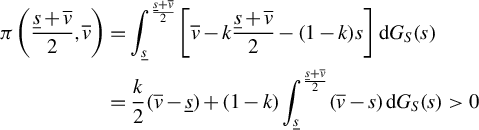 $$\begin{align*}\pi\left(\frac{\underline{s}+\overline{v}}{2},\overline{v}\right) &= \int_{\underline{s}}^{\frac{\underline{s}+\overline{v}}{2}}\left[\overline{v}-k\frac{\underline{s}+\overline{v}}{2}-(1-k)s\right]\,\mathrm{d} G_S(s)\\ & = \frac{k}{2}(\overline{v}-\underline{s})+(1-k)\int_{\underline{s}}^{\frac{\underline{s}+\overline{v}}{2}}(\overline{v}-s)\,\mathrm{d} G_S(s)>0\end{align*}$$
while bidding $\overline {b}\leq \underline {s}$
gives him zero expected profit. This contradicts the equilibrium requirement. (ii) If
$\overline {b}\leq \underline {s}$
gives him zero expected profit. This contradicts the equilibrium requirement. (ii) If $\underline {c}<\overline {b}\leq \underline {s}$
, then an analogous argument can show that bidding
$\underline {c}<\overline {b}\leq \underline {s}$
, then an analogous argument can show that bidding $\frac {\overline {b}+\underline {c}}{2}$
is a profitable deviation for the seller with value
$\frac {\overline {b}+\underline {c}}{2}$
is a profitable deviation for the seller with value $\underline {c}$
, which also presents a contradiction to the equilibrium condition. (iii) If
$\underline {c}$
, which also presents a contradiction to the equilibrium condition. (iii) If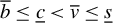 $\overline {b}\leq \underline {c}<\overline {v}\leq \underline {s}$
, then condition A3 of Assumption C is contradicted because it requires that
$\overline {b}\leq \underline {c}<\overline {v}\leq \underline {s}$
, then condition A3 of Assumption C is contradicted because it requires that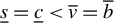 $\underline {s}=\underline {c}<\overline {v}=\overline {b}$
. From the above, C1 holds.
$\underline {s}=\underline {c}<\overline {v}=\overline {b}$
. From the above, C1 holds.
Because V and C are independent and because $\beta _B(\mkern 2mu\cdot \mkern 2mu)$
and
$\beta _B(\mkern 2mu\cdot \mkern 2mu)$
and $\beta _S(\mkern 2mu\cdot \mkern 2mu)$
are deterministic functions, it follows that the bids,
$\beta _S(\mkern 2mu\cdot \mkern 2mu)$
are deterministic functions, it follows that the bids, $B=\beta _B(V)$
and
$B=\beta _B(V)$
and $S=\beta _S(C)$
, are also independent. More precisely, since
$S=\beta _S(C)$
, are also independent. More precisely, since $\beta _B(\mkern 2mu\cdot \mkern 2mu)$
and
$\beta _B(\mkern 2mu\cdot \mkern 2mu)$
and $\beta _S(\mkern 2mu\cdot \mkern 2mu)$
are continuous and strictly increasing, there exist inverse functions,
$\beta _S(\mkern 2mu\cdot \mkern 2mu)$
are continuous and strictly increasing, there exist inverse functions, $\beta _B^{-1}(\mkern 2mu\cdot \mkern 2mu)$
and
$\beta _B^{-1}(\mkern 2mu\cdot \mkern 2mu)$
and $\beta _S^{-1}(\mkern 2mu\cdot \mkern 2mu)$
, which are also continuous and strictly increasing. Thus,
$\beta _S^{-1}(\mkern 2mu\cdot \mkern 2mu)$
, which are also continuous and strictly increasing. Thus,
 $$ \begin{align*} G(b,s) &= \Pr(\beta_B(V)\leq b, \beta_S(C)\leq s)\\ &= \Pr(V\leq \beta_B^{-1}(b), C\leq \beta_S^{-1}(s))\\ &= \Pr(V\leq \beta_B^{-1}(b))\Pr(C\leq \beta_S^{-1}(s))=F_V(\beta_B^{-1}(b))F_C(\beta_S^{-1}(s)). \end{align*} $$
Define
 $$ \begin{align} G_B(b)&=F_V(\beta_B^{-1}(b)) \end{align} $$
 $$ \begin{align} G_S(s)&=F_C(\beta_S^{-1}(s)) \end{align} $$
for every $b\in [\underline {b}, \overline {b}]$
and
$b\in [\underline {b}, \overline {b}]$
and $s\in [\underline {s}, \overline {s}]$
. Since
$s\in [\underline {s}, \overline {s}]$
. Since $\beta _B^{-1}(\mkern 2mu\cdot \mkern 2mu)$
is continuous and strictly increasing in
$\beta _B^{-1}(\mkern 2mu\cdot \mkern 2mu)$
is continuous and strictly increasing in $[\underline {b}, \overline {b}]=[\beta _B(\underline {v}), \beta _B(\overline {v})]$
, we have
$[\underline {b}, \overline {b}]=[\beta _B(\underline {v}), \beta _B(\overline {v})]$
, we have $G_B\in \mathscr {P}_{[\underline {b}, \overline {b}]}$
by (A.6) and the assumption
$G_B\in \mathscr {P}_{[\underline {b}, \overline {b}]}$
by (A.6) and the assumption $F_V\in \mathscr {P}_{[\underline {v}, \overline {v}]}$
. Similar argument can be applied to show
$F_V\in \mathscr {P}_{[\underline {v}, \overline {v}]}$
. Similar argument can be applied to show $G_S\in \mathscr {P}_{[\underline {s}, \overline {s}]}$
. Now, we get C2.
$G_S\in \mathscr {P}_{[\underline {s}, \overline {s}]}$
. Now, we get C2.
In order to show C3 and C4, note that $G_B(\mkern 2mu\cdot \mkern 2mu)$
and
$G_B(\mkern 2mu\cdot \mkern 2mu)$
and $G_S(\mkern 2mu\cdot \mkern 2mu)$
defined in (A.6) and (A.7) must be the distributions of observed (equilibrium) bids of the buyer and the seller, respectively. Now,
$G_S(\mkern 2mu\cdot \mkern 2mu)$
defined in (A.6) and (A.7) must be the distributions of observed (equilibrium) bids of the buyer and the seller, respectively. Now, $\beta _B(\mkern 2mu\cdot \mkern 2mu)$
and
$\beta _B(\mkern 2mu\cdot \mkern 2mu)$
and $\beta _S(\mkern 2mu\cdot \mkern 2mu)$
must solve the set of first-order differential equations (3.5) and (3.6). Since (3.7) and (3.8) follow from (3.5) and (3.6),
$\beta _S(\mkern 2mu\cdot \mkern 2mu)$
must solve the set of first-order differential equations (3.5) and (3.6). Since (3.7) and (3.8) follow from (3.5) and (3.6), $\beta _B(\mkern 2mu\cdot \mkern 2mu)$
and
$\beta _B(\mkern 2mu\cdot \mkern 2mu)$
and $\beta _S(\mkern 2mu\cdot \mkern 2mu)$
must satisfy
$\beta _S(\mkern 2mu\cdot \mkern 2mu)$
must satisfy
 $$\begin{align*}\xi(\beta_B(v),G_S)=v,\quad \eta(\beta_S(c),G_B)=c\end{align*}$$
for all $v\geq \underline {s}$
and all
$v\geq \underline {s}$
and all $c\leq \overline {b}$
. Noting that
$c\leq \overline {b}$
. Noting that $\underline {s}=\beta _S(\underline {c})$
and
$\underline {s}=\beta _S(\underline {c})$
and $\overline {b}=\beta _B(\overline {v})$
and making the change of variable
$\overline {b}=\beta _B(\overline {v})$
and making the change of variable $v=\beta _B^{-1}(b)$
and
$v=\beta _B^{-1}(b)$
and $c=\beta _S^{-1}(s)$
, we obtain
$c=\beta _S^{-1}(s)$
, we obtain
 $$ \begin{align} \xi(b,G_S)=\beta_B^{-1}(b) \end{align} $$
 $$ \begin{align} \eta(s,G_B)=\beta_S^{-1}(s) \end{align} $$
for all $b,s\in [\underline {s},\overline {b}]$
. By condition A1 of Assumption C, both
$b,s\in [\underline {s},\overline {b}]$
. By condition A1 of Assumption C, both $\beta _B^{-1}(\mkern 2mu\cdot \mkern 2mu)$
and
$\beta _B^{-1}(\mkern 2mu\cdot \mkern 2mu)$
and $\beta _S^{-1}(\mkern 2mu\cdot \mkern 2mu)$
are strictly increasing, and by condition A3 of Assumption C,
$\beta _S^{-1}(\mkern 2mu\cdot \mkern 2mu)$
are strictly increasing, and by condition A3 of Assumption C, $\beta _B(\mkern 2mu\cdot \mkern 2mu)$
is differentiable on
$\beta _B(\mkern 2mu\cdot \mkern 2mu)$
is differentiable on $[\underline {s},\overline {v}]$
and so is
$[\underline {s},\overline {v}]$
and so is $\beta _S(\mkern 2mu\cdot \mkern 2mu)$
on
$\beta _S(\mkern 2mu\cdot \mkern 2mu)$
on $[\underline {c},\overline {b}]$
. Thus, C3 and C4 follow from the fact that
$[\underline {c},\overline {b}]$
. Thus, C3 and C4 follow from the fact that $\xi (\underline {s},G_S)=\underline {s}$
by (3.7),
$\xi (\underline {s},G_S)=\underline {s}$
by (3.7),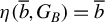 $\eta (\overline {b},G_B)=\overline {b}$
by (3.8), and
$\eta (\overline {b},G_B)=\overline {b}$
by (3.8), and $\overline {v}=\beta _B^{-1}(\overline {b})=\xi (\overline {b},G_S)$
,
$\overline {v}=\beta _B^{-1}(\overline {b})=\xi (\overline {b},G_S)$
, $\underline {c}=\beta _S^{-1}(\underline {s})=\eta (\underline {s},G_B)$
.
$\underline {c}=\beta _S^{-1}(\underline {s})=\eta (\underline {s},G_B)$
.
It remains to show C5 and C6. Given $b\in [\underline s,\overline {b}]$
, for the buyer with private value v such that
$b\in [\underline s,\overline {b}]$
, for the buyer with private value v such that $\beta _B(v)=b$
, bidding any
$\beta _B(v)=b$
, bidding any $b'\in [\overline {b},\overline {s}]$
should not give him greater profit than bidding b because
$b'\in [\overline {b},\overline {s}]$
should not give him greater profit than bidding b because $\beta _B$
is the equilibrium bidding strategy for the buyer. That is,
$\beta _B$
is the equilibrium bidding strategy for the buyer. That is,
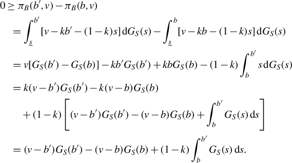 $$ \begin{align*} & 0\geq \pi_B(b',v)-\pi_B(b,v) \\ & \quad = \int_{\underline{s}}^{b'} [v-kb'-(1-k)s]\,\mathrm{d} G_S(s) - \int_{\underline{s}}^{b}[v-kb-(1-k)s]\,\mathrm{d} G_S(s) \\ &\quad = v[G_S(b')-G_S(b)] -kb'G_S(b')+kbG_S(b)-(1-k)\int_b^{b'}s\,\mathrm{d} G_S(s)\\ &\quad = k(v-b')G_S(b')-k(v-b)G_S(b) \\ &\qquad + (1-k)\left[(v-b')G_S(b')-(v-b)G_S(b)+\int_b^{b'}G_S(s)\,\mathrm{d} s\right]\\ &\quad = (v-b')G_S(b')-(v-b)G_S(b)+(1-k)\int_b^{b'}G_S(s)\,\mathrm{d} s. \end{align*} $$
Because $v=\beta _B^{-1}(b)=\xi (b,G_S)$
by (A.8), replacing v by
$v=\beta _B^{-1}(b)=\xi (b,G_S)$
by (A.8), replacing v by $\xi (b,G_S)$
in the above inequality will give (3.11). Similarly, for the seller with private value c such that
$\xi (b,G_S)$
in the above inequality will give (3.11). Similarly, for the seller with private value c such that $\beta _S(c)=s\in [\underline {s},\overline b]$
, using the argument that any deviation of bidding
$\beta _S(c)=s\in [\underline {s},\overline b]$
, using the argument that any deviation of bidding $s'\in [\underline {b},\underline {s}]$
would not be profitable, we can show that (3.12) must hold. This completes the proof of C6 and the theorem.
$s'\in [\underline {b},\underline {s}]$
would not be profitable, we can show that (3.12) must hold. This completes the proof of C6 and the theorem.
A.5 Proof of Theorem 2
We show the identification of $F_V$
and
$F_V$
and $F_C$
in two steps. In the first step, we construct a pair of
$F_C$
in two steps. In the first step, we construct a pair of $F_V$
and
$F_V$
and $F_C$
to rationalize the given G. In the second step, we show that this pair is unique.
$F_C$
to rationalize the given G. In the second step, we show that this pair is unique.
Step 1. To show the sufficiency of C1–C4, define
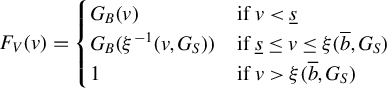 $$ \begin{align} F_V(v)=\begin{cases} G_B(v) & \text{if } v<\underline{s}\\ G_B(\xi^{-1}(v,G_S)) & \text{if } \underline{s}\leq v\leq \xi(\overline{b},G_S)\\ 1 & \text{if } v>\xi(\overline{b},G_S) \end{cases} \end{align} $$
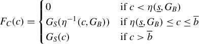 $$ \begin{align} F_C(c)=\begin{cases} 0 & \text{if } c<\eta(\underline{s},G_B)\\ G_S(\eta^{-1}(c,G_B)) & \text{if } \eta(\underline{s},G_B)\leq c\leq\overline{b}\\ G_S(c) & \text{if } c>\overline{b} \end{cases} \end{align} $$
and
 $$\begin{align*}\underline{v}=\underline{b},\quad \overline{v}=\xi(\overline{b},G_S),\quad \underline{c}=\eta(\underline{s},G_B),\quad \overline{c}=\overline{s}.\end{align*}$$
Condition C1 guarantees that the functions $\xi (\mkern 2mu\cdot \mkern 2mu,G_S)$
in (3.7) and
$\xi (\mkern 2mu\cdot \mkern 2mu,G_S)$
in (3.7) and $\eta (\mkern 2mu\cdot \mkern 2mu,G_S)$
in (3.8) are well defined. Since
$\eta (\mkern 2mu\cdot \mkern 2mu,G_S)$
in (3.8) are well defined. Since $\underline {b}$
is the lower end point of the support of
$\underline {b}$
is the lower end point of the support of $G_B$
, for all
$G_B$
, for all $v\leq \underline {v}=\underline {b}$
,
$v\leq \underline {v}=\underline {b}$
, $F_V(v)=0$
, and by definition,
$F_V(v)=0$
, and by definition, $F_V(v)=1$
for all
$F_V(v)=1$
for all $v>\overline {v}=\xi (\overline {b},G_S)$
. Moreover, because
$v>\overline {v}=\xi (\overline {b},G_S)$
. Moreover, because $F_V(\overline {v})=G_B(\xi ^{-1}(\xi (\overline {b},G_S),G_S))=G_B(\overline {b})=1$
,
$F_V(\overline {v})=G_B(\xi ^{-1}(\xi (\overline {b},G_S),G_S))=G_B(\overline {b})=1$
, $F_V(\underline {s}) = G_B(\xi ^{-1}(\xi (\underline {s},G_S),G_S)) = G_B(\underline {s})$
,
$F_V(\underline {s}) = G_B(\xi ^{-1}(\xi (\underline {s},G_S),G_S)) = G_B(\underline {s})$
, $G_B$
is continuous and strictly increasing on
$G_B$
is continuous and strictly increasing on $[\underline {b},\overline {b}]$
by C2, and
$[\underline {b},\overline {b}]$
by C2, and $\xi ^{-1}(\mkern 2mu\cdot \mkern 2mu,G_S)$
is continuous and strictly increasing on
$\xi ^{-1}(\mkern 2mu\cdot \mkern 2mu,G_S)$
is continuous and strictly increasing on $[\xi (\underline {s},G_S),\xi (\overline {b},G_S)]$
by C3. Then
$[\xi (\underline {s},G_S),\xi (\overline {b},G_S)]$
by C3. Then $F_V(\mkern 2mu\cdot \mkern 2mu)$
defined by (A.10) is continuous and strictly increasing in
$F_V(\mkern 2mu\cdot \mkern 2mu)$
defined by (A.10) is continuous and strictly increasing in $[\underline {b},\xi (\overline {b},G_S)]=[\underline {v},\overline {v}]$
. Therefore,
$[\underline {b},\xi (\overline {b},G_S)]=[\underline {v},\overline {v}]$
. Therefore, $F_V$
is a valid absolutely continuous distribution with support
$F_V$
is a valid absolutely continuous distribution with support $[\underline {v},\overline {v}]$
, that is,
$[\underline {v},\overline {v}]$
, that is, $F_V\in \mathscr {P}_{[\underline {v},\overline {v}]}$
as required. We can also show
$F_V\in \mathscr {P}_{[\underline {v},\overline {v}]}$
as required. We can also show $F_C\in \mathscr {P}_{[\underline {c},\overline {c}]}$
in a similar way.
$F_C\in \mathscr {P}_{[\underline {c},\overline {c}]}$
in a similar way.
We shall show that the distributions $F_V$
and
$F_V$
and $F_C$
of the respective private values of the buyer and the seller can rationalize G in a sealed-bid k-double auction, that is,
$F_C$
of the respective private values of the buyer and the seller can rationalize G in a sealed-bid k-double auction, that is, $G_B(b)=F_V(\beta _B^{-1}(b))$
in
$G_B(b)=F_V(\beta _B^{-1}(b))$
in $[\underline {b},\overline {b}]$
and
$[\underline {b},\overline {b}]$
and $G_S(s)=F_C(\beta _S^{-1}(s))$
on
$G_S(s)=F_C(\beta _S^{-1}(s))$
on $[\underline {s},\overline {s}]$
for some regular equilibrium profile
$[\underline {s},\overline {s}]$
for some regular equilibrium profile $(\beta _B,\beta _S)$
. By construction of
$(\beta _B,\beta _S)$
. By construction of $F_V$
and
$F_V$
and $F_C$
, we have
$F_C$
, we have
 $$ \begin{align*} G_B(b) & =F_V(b) \mathbb{1}(\underline{b}\leq b<\underline{s})+F_V(\xi(b,G_S)) \mathbb{1}(\underline{s}\leq b\leq\overline{b})\\ & =F_V\left(b \mathbb{1}(\underline{b}\leq b<\underline{s})+\xi(b,G_S) \mathbb{1}(\underline{s}\leq b\leq\overline{b})\right) \end{align*} $$
for $b\in [\underline {b},\overline {b}]$
and
$b\in [\underline {b},\overline {b}]$
and
 $$ \begin{align*} G_S(s) & =F_C(\eta(s,G_B)) \mathbb{1}(\underline{s}\leq s\leq \overline{b}) + F_C(s) \mathbb{1}(\overline{b}<s\leq\overline{s})\\ & =F_C\left(\eta(s,G_B) \mathbb{1}(\underline{s}\leq s\leq \overline{b}) + s \mathbb{1}(\overline{b}<s\leq\overline{s})\right) \end{align*} $$
for $s\in [\underline {s},\overline {s}]$
, where
$s\in [\underline {s},\overline {s}]$
, where $\mathbb {1}(\mkern 2mu\cdot \mkern 2mu)$
is the indicator function. Define
$\mathbb {1}(\mkern 2mu\cdot \mkern 2mu)$
is the indicator function. Define
 $$ \begin{align*} \xi_*(b,G_S) &\equiv b \mathbb{1}(\underline{b}\leq b<\underline{s})+\xi(b,G_S)\mathbb{1}(\underline{s}\leq b\leq\overline{b}),\\ \eta_*(s,G_B) &\equiv \eta(s,G_B)\mathbb{1}(\underline{s}\leq s\leq \overline{b})+s \mathbb{1}(\overline{b}<s\leq\overline{s}), \end{align*} $$
then by C3 and C4, $\xi _*(\mkern 2mu\cdot \mkern 2mu,G_S)$
is continuous and strictly increasing on
$\xi _*(\mkern 2mu\cdot \mkern 2mu,G_S)$
is continuous and strictly increasing on $[\underline {b},\overline {b}]$
and so is
$[\underline {b},\overline {b}]$
and so is $\eta _*(\mkern 2mu\cdot \mkern 2mu,G_B)$
on
$\eta _*(\mkern 2mu\cdot \mkern 2mu,G_B)$
on $[\underline {s},\overline {s}]$
. Define bidding strategies
$[\underline {s},\overline {s}]$
. Define bidding strategies
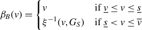 $$ \begin{align} \beta_B(v) &= \begin{cases} v & \text{if } \underline{v}\leq v \leq \underline{s}\\ \xi^{-1}(v,G_S) & \text{if } \underline{s}<v\leq\overline{v} \end{cases} \end{align} $$
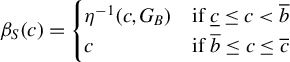 $$ \begin{align} \beta_S(c) &= \begin{cases} \eta^{-1}(c,G_B) & \text{if } \underline{c}\leq c <\overline{b}\\ c & \text{if } \overline{b}\leq c\leq\overline{c} \end{cases} \end{align} $$
so that $\beta _B(\mkern 2mu\cdot \mkern 2mu)=\xi _*^{-1}(\mkern 2mu\cdot \mkern 2mu,G_S)$
and
$\beta _B(\mkern 2mu\cdot \mkern 2mu)=\xi _*^{-1}(\mkern 2mu\cdot \mkern 2mu,G_S)$
and $\beta _S(\mkern 2mu\cdot \mkern 2mu)=\eta _*^{-1}(\mkern 2mu\cdot \mkern 2mu,G_B)$
. By construction of these strategies, A1–A3 in Assumption C are satisfied, and also
$\beta _S(\mkern 2mu\cdot \mkern 2mu)=\eta _*^{-1}(\mkern 2mu\cdot \mkern 2mu,G_B)$
. By construction of these strategies, A1–A3 in Assumption C are satisfied, and also $G_B(b)=F_V(\beta _B^{-1}(b))$
and
$G_B(b)=F_V(\beta _B^{-1}(b))$
and $G_S(s)=F_C(\beta _S^{-1}(s))$
so that G is the induced bid distribution for
$G_S(s)=F_C(\beta _S^{-1}(s))$
so that G is the induced bid distribution for $(F_V,F_C)$
defined in (A.10) and (A.11) by the strategy profile
$(F_V,F_C)$
defined in (A.10) and (A.11) by the strategy profile $(\beta _B,\beta _S)$
defined above. Thus, it remains to show that
$(\beta _B,\beta _S)$
defined above. Thus, it remains to show that $(\beta _B,\beta _S)$
is indeed an equilibrium. We show that the optimal offer for the buyer with private value v is
$(\beta _B,\beta _S)$
is indeed an equilibrium. We show that the optimal offer for the buyer with private value v is $\beta _B(v)$
. A similar argument shows that
$\beta _B(v)$
. A similar argument shows that $\beta _S$
is optimal for the seller.
$\beta _S$
is optimal for the seller.
Obviously, if $v\leq \underline {s}$
, then the buyer cannot make an advantageous trade and bidding
$v\leq \underline {s}$
, then the buyer cannot make an advantageous trade and bidding $\beta _B(v)=v$
achieves zero as the greatest possible expected profit. Suppose
$\beta _B(v)=v$
achieves zero as the greatest possible expected profit. Suppose $v>\underline {s}$
, since
$v>\underline {s}$
, since $G_S$
is the induced seller’s bid distribution, for bid
$G_S$
is the induced seller’s bid distribution, for bid $b\in [\underline {s},\overline {b}]$
, by (2.1), we obtain
$b\in [\underline {s},\overline {b}]$
, by (2.1), we obtain
 $$ \begin{align*} \frac{\partial\pi_B(b,s)}{\partial b} &= -k G_S(b) + (v-kb)g_S(b) - (1-k)bg_S(b) \\ &= g_S(b)\left[v-\left(b+k\frac{G_S(b)}{g_S(b)}\right)\right] = g_S(b)\left[v-\xi(b,G_S)\right]. \end{align*} $$
Because $g_S(b)$
is positive, the monotonicity of
$g_S(b)$
is positive, the monotonicity of $\xi (\mkern 2mu\cdot \mkern 2mu,G_S)$
by C3 implies that
$\xi (\mkern 2mu\cdot \mkern 2mu,G_S)$
by C3 implies that $\partial \pi _B(b,v)/\partial b>0$
for all
$\partial \pi _B(b,v)/\partial b>0$
for all $b<\xi ^{-1}(v,G_S)$
and
$b<\xi ^{-1}(v,G_S)$
and $\partial \pi _B(b,v)/\partial b<0$
for all
$\partial \pi _B(b,v)/\partial b<0$
for all $b>\xi ^{-1}(v,G_S)$
. Therefore,
$b>\xi ^{-1}(v,G_S)$
. Therefore, $b=\xi ^{-1}(v,G_S)=\beta _B(v)$
is the unique maximizer of the expected profit of the buyer in
$b=\xi ^{-1}(v,G_S)=\beta _B(v)$
is the unique maximizer of the expected profit of the buyer in $[\underline {s},\overline {b}]$
. Now, we show that the buyer would not want to choose a bid within
$[\underline {s},\overline {b}]$
. Now, we show that the buyer would not want to choose a bid within $[\overline {b},\overline {s}]$
, either. Recall that we have already shown that C5 is equivalent to
$[\overline {b},\overline {s}]$
, either. Recall that we have already shown that C5 is equivalent to $\pi _B(b',v)\leq \pi _B(b,v)$
for any
$\pi _B(b',v)\leq \pi _B(b,v)$
for any $v\in [\underline s,\xi (\overline {b},G_S)]$
and any
$v\in [\underline s,\xi (\overline {b},G_S)]$
and any $b'\in [\overline {b},\overline {s}]$
when
$b'\in [\overline {b},\overline {s}]$
when $b=\xi ^{-1}(v,G_S)=\beta _B(v)$
in the proof of Theorem 1, so the buyer is not profitable to deviate from
$b=\xi ^{-1}(v,G_S)=\beta _B(v)$
in the proof of Theorem 1, so the buyer is not profitable to deviate from $b\in [\underline s,\overline b]$
to
$b\in [\underline s,\overline b]$
to $b'\in [\overline b,\overline s]$
. Finally, given that
$b'\in [\overline b,\overline s]$
. Finally, given that $\overline {s}$
is the highest bid of the seller, any buyer’s bid greater than
$\overline {s}$
is the highest bid of the seller, any buyer’s bid greater than $\overline {s}$
will be dominated by
$\overline {s}$
will be dominated by $\overline {s}$
. Hence,
$\overline {s}$
. Hence, $F_V$
and
$F_V$
and $F_C$
rationalize G in a sealed bid k-double auction.
$F_C$
rationalize G in a sealed bid k-double auction.
Step 2. From the proof of Theorem 1, we know that $\xi (\mkern 2mu\cdot \mkern 2mu,G_S)=\beta _B^{-1}(\mkern 2mu\cdot \mkern 2mu)$
and
$\xi (\mkern 2mu\cdot \mkern 2mu,G_S)=\beta _B^{-1}(\mkern 2mu\cdot \mkern 2mu)$
and $\eta (\mkern 2mu\cdot \mkern 2mu,G_B)=\beta _S^{-1}(\mkern 2mu\cdot \mkern 2mu)$
on
$\eta (\mkern 2mu\cdot \mkern 2mu,G_B)=\beta _S^{-1}(\mkern 2mu\cdot \mkern 2mu)$
on $[\underline {s},\overline {b}]$
when
$[\underline {s},\overline {b}]$
when $F_V(\mkern 2mu\cdot \mkern 2mu)$
and
$F_V(\mkern 2mu\cdot \mkern 2mu)$
and $F_C(\mkern 2mu\cdot \mkern 2mu)$
exist. Since
$F_C(\mkern 2mu\cdot \mkern 2mu)$
exist. Since $F_V(\mkern 2mu\cdot \mkern 2mu)=G_B(\beta _B(\mkern 2mu\cdot \mkern 2mu))$
and
$F_V(\mkern 2mu\cdot \mkern 2mu)=G_B(\beta _B(\mkern 2mu\cdot \mkern 2mu))$
and $F_C(\mkern 2mu\cdot \mkern 2mu)=G_S(\beta _S(\mkern 2mu\cdot \mkern 2mu))$
,
$F_C(\mkern 2mu\cdot \mkern 2mu)=G_S(\beta _S(\mkern 2mu\cdot \mkern 2mu))$
, $F_V(\mkern 2mu\cdot \mkern 2mu)=G_B(\xi _*^{-1}(\mkern 2mu\cdot \mkern 2mu,G_S))$
and
$F_V(\mkern 2mu\cdot \mkern 2mu)=G_B(\xi _*^{-1}(\mkern 2mu\cdot \mkern 2mu,G_S))$
and $F_C(\mkern 2mu\cdot \mkern 2mu)=G_S(\eta _*^{-1}(\mkern 2mu\cdot \mkern 2mu,G_B))$
. Because
$F_C(\mkern 2mu\cdot \mkern 2mu)=G_S(\eta _*^{-1}(\mkern 2mu\cdot \mkern 2mu,G_B))$
. Because $\xi (\mkern 2mu\cdot \mkern 2mu,G_S)$
is uniquely determined by
$\xi (\mkern 2mu\cdot \mkern 2mu,G_S)$
is uniquely determined by $G_S(\mkern 2mu\cdot \mkern 2mu)$
and
$G_S(\mkern 2mu\cdot \mkern 2mu)$
and $\eta (\mkern 2mu\cdot \mkern 2mu,G_B)$
is uniquely determined by
$\eta (\mkern 2mu\cdot \mkern 2mu,G_B)$
is uniquely determined by $G_B(\mkern 2mu\cdot \mkern 2mu)$
, it follows that
$G_B(\mkern 2mu\cdot \mkern 2mu)$
, it follows that $\xi _*(\mkern 2mu\cdot \mkern 2mu,G_S)$
and
$\xi _*(\mkern 2mu\cdot \mkern 2mu,G_S)$
and $\eta _*(\mkern 2mu\cdot \mkern 2mu,G_B)$
are uniquely determined by G. Hence, the private value distribution
$\eta _*(\mkern 2mu\cdot \mkern 2mu,G_B)$
are uniquely determined by G. Hence, the private value distribution $(F_V,F_C)$
that rationalizes G is unique.
$(F_V,F_C)$
that rationalizes G is unique.
This therefore establishes the identification of $F_V$
and
$F_V$
and $F_C$
from any given
$F_C$
from any given $G\in {\mathscr P}_{\mathscr D}$
satisfying C1–C6.
$G\in {\mathscr P}_{\mathscr D}$
satisfying C1–C6.
A.6 Proof of Theorem 4
It is straightforward to see that conditions C3 and C4 are implied by C7 and C8. Then it suffices to show that C5 and C6 are implied by C7 and C8.
We shall only show that C7 (more precisely, the monotonicity of $\xi (\mkern 2mu\cdot \mkern 2mu,G_S)$
) implies C5. A similar argument can show that C8 implies C6. For the buyer with private value v, since
$\xi (\mkern 2mu\cdot \mkern 2mu,G_S)$
) implies C5. A similar argument can show that C8 implies C6. For the buyer with private value v, since
 $$\begin{align*}\frac{\partial\pi_B(b,v)}{\partial b} = g_S(b)\left[v-\xi(b,G_S)\right],\end{align*}$$
the strict monotonicity of $\xi (\mkern 2mu\cdot \mkern 2mu,G_S)$
in
$\xi (\mkern 2mu\cdot \mkern 2mu,G_S)$
in $[\underline {s},\overline {s}]$
ensures that for any
$[\underline {s},\overline {s}]$
ensures that for any $b\in \left (\xi ^{-1}(v,G_S),\overline {s}\right ]$
,
$b\in \left (\xi ^{-1}(v,G_S),\overline {s}\right ]$
, $\partial \pi _B(b,v)/\partial b<0$
. As a result, the expected profit of the buyer
$\partial \pi _B(b,v)/\partial b<0$
. As a result, the expected profit of the buyer $\pi _B(b,v)$
is strictly decreasing in the buyer’s bid for all
$\pi _B(b,v)$
is strictly decreasing in the buyer’s bid for all $b\in (\xi ^{-1}(v,G_S),\overline s]$
. For
$b\in (\xi ^{-1}(v,G_S),\overline s]$
. For $b'\in [\overline {b},\overline {s}]$
and
$b'\in [\overline {b},\overline {s}]$
and $b\in [\underline s,\overline b]$
, let
$b\in [\underline s,\overline b]$
, let $v=\xi (b,G_S)$
, then it follows from the above conclusion that
$v=\xi (b,G_S)$
, then it follows from the above conclusion that
 $$\begin{align*}b'\geq\overline{b}\geq b=\xi^{-1}(v,G_S)\quad\Rightarrow\quad \pi_B(b',v)\leq \pi_B(b,v), \end{align*}$$
which is equivalent to C5 as shown in the proof of Theorem 1.
A.7 Proof of Theorem 3
By Theorem 1, C1–C4 hold. Let $m' = \Pr (\underline {s}\leq S \leq B\leq \overline {b})$
. By the definition of
$m' = \Pr (\underline {s}\leq S \leq B\leq \overline {b})$
. By the definition of $G_2$
, D1 is the direct corollary of C1. Using
$G_2$
, D1 is the direct corollary of C1. Using $g_2(b,s)=g(b,s)/m'$
and
$g_2(b,s)=g(b,s)/m'$
and $g(b,s)=g_B(b)g_S(s)$
by C2, we have
$g(b,s)=g_B(b)g_S(s)$
by C2, we have
 $$ \begin{align*}g_{2}(b,s)g_{2}(b',s')=g_{2}(b,s')g_{2}(b',s)=\frac{g_{B}(b)g_{B}(b')g_{S}(s)g_{S}(s')}{m^{'2}}, \end{align*} $$
so D2 is satisfied. D3 and D4 are implied by C3 and C4, respectively.
A.8 Proof of Theorem 4
By condition D1 and Lemma 1, we have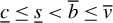 $\underline {c}\leq \underline {s}<\overline {b}\leq \overline {v}$
, namely, condition E1 is satisfied.
$\underline {c}\leq \underline {s}<\overline {b}\leq \overline {v}$
, namely, condition E1 is satisfied.
Notice that, by D3 and D4, (3.13) is equivalent to
 $$ \begin{align} \frac{F_V(\xi(b,G_{S}))-F_V(\underline{s})}{1-F_V(\underline{s})}= \frac{G_B(b)-G_B(\underline{s})}{1-G_B(\underline{s})} ,\quad \frac{F_C(\eta(s,G_{B}))}{F_C(\overline{b})}=\frac{G_S(s)}{G_S(\overline{b})} \end{align} $$
for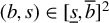 $(b,s)\in [\underline {s},\overline {b}]^2$
.
$(b,s)\in [\underline {s},\overline {b}]^2$
.
Next, we establish condition E2 by showing (A.14). According to the proof of Theorem 2, G can only be rationalized by $(F_V,F_C)$
defined in (A.10) and (A.11) which implies
$(F_V,F_C)$
defined in (A.10) and (A.11) which implies
 $$ \begin{align} F_V(\xi(b,G_S))=G_B(b),\quad F_C(\eta(s,G_B))=G_S(s) \end{align} $$
for $\underline {s}=\xi ^{-1}(\underline {s},G_S)\leq b\leq \overline {b}$
and
$\underline {s}=\xi ^{-1}(\underline {s},G_S)\leq b\leq \overline {b}$
and $\underline {s}\leq s\leq \eta ^{-1}(\overline {b},G_B)=\overline {b}$
. By (A.15) and using
$\underline {s}\leq s\leq \eta ^{-1}(\overline {b},G_B)=\overline {b}$
. By (A.15) and using $\xi (\underline {s},G_{S})=\underline {s}$
,
$\xi (\underline {s},G_{S})=\underline {s}$
,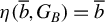 $\eta (\overline {b},G_{B})=\overline {b}$
, we have condition (A.14) to hold for all
$\eta (\overline {b},G_{B})=\overline {b}$
, we have condition (A.14) to hold for all $F_V$
and
$F_V$
and $F_C$
. We therefore establish condition E2 and complete the entire proof.
$F_C$
. We therefore establish condition E2 and complete the entire proof.
A.9 Proof of Theorem 4
We will only show the identification of $\theta _B$
. The case of
$\theta _B$
. The case of $\theta _S$
can be proved in a similar way.
$\theta _S$
can be proved in a similar way.
Let ${\mathcal B}(v_j) \equiv \big [G_B(\xi ^{-1}(v_j,G_{S})) - G_{B}(\underline {s})\big ]\big /\big (1-G_B(\underline {s})\big ) $
and
${\mathcal B}(v_j) \equiv \big [G_B(\xi ^{-1}(v_j,G_{S})) - G_{B}(\underline {s})\big ]\big /\big (1-G_B(\underline {s})\big ) $
and $\phi _j(\theta _{B}) \equiv {\mathcal Q}_B(\theta _{B};v_j) - {\mathcal B}(v_j)$
for
$\phi _j(\theta _{B}) \equiv {\mathcal Q}_B(\theta _{B};v_j) - {\mathcal B}(v_j)$
for $j = 1,\dots ,m$
. By Condition E.2 of Theorem 4, we have
$j = 1,\dots ,m$
. By Condition E.2 of Theorem 4, we have $\phi _j(\theta _{B}) = 0$
for all
$\phi _j(\theta _{B}) = 0$
for all $\theta _B\in \Theta _B'$
and
$\theta _B\in \Theta _B'$
and $j=1,\dots ,m$
. Notice that the Jacobian matrix of
$j=1,\dots ,m$
. Notice that the Jacobian matrix of $(\phi _1(\theta _{B}),\dots ,\phi _m(\theta _{B}))$
w.r.t.
$(\phi _1(\theta _{B}),\dots ,\phi _m(\theta _{B}))$
w.r.t. $\theta _B$
is
$\theta _B$
is $J{\mathcal Q}_B(\theta _B;v^m)$
. The desired conclusion therefore follows from Theorem 7 of Rothenberg (Reference Rothenberg1971).
$J{\mathcal Q}_B(\theta _B;v^m)$
. The desired conclusion therefore follows from Theorem 7 of Rothenberg (Reference Rothenberg1971).
A.10 Proof of Lemma 5
Part (i) follows directly from Lemma 7 given that the bandwidths $h_B$
and
$h_B$
and $h_S$
satisfy Assumption G. We next show part (ii). We shall show the convergence rate of
$h_S$
satisfy Assumption G. We next show part (ii). We shall show the convergence rate of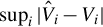 $\sup _i |\hat {V}_i-V_i|$
. The result for
$\sup _i |\hat {V}_i-V_i|$
. The result for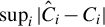 $\sup _i |\hat {C}_i-C_i|$
can be shown analogously.
$\sup _i |\hat {C}_i-C_i|$
can be shown analogously.
It follows from the definition of $\xi (b,G_S)$
and (4.3) that
$\xi (b,G_S)$
and (4.3) that
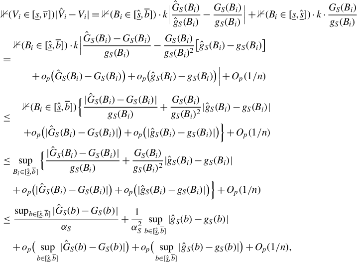 $$ \begin{align} &\mathbb{1}(V_i\in[\underline{s},\overline{v}]) |\hat{V}_i-V_i| = \mathbb{1}(B_i\in [\hat{\underline{s}},\overline{b}])\cdot k\Big|\frac{\hat{G}_S(B_i)}{\hat{g}_S(B_i)}-\frac{G_S(B_i)}{g_S(B_i)}\Big| + \mathbb{1}(B_i\in [\underline{s},\hat{\underline{s}}])\cdot k\cdot\frac{G_S(B_i)}{g_S(B_i)} \nonumber \\ &= \begin{aligned} \mathbb{1}(B_i\in [\hat{\underline{s}},\overline{b}])\cdot k\Big|\frac{\hat{G}_S(B_i)-G_S(B_i)}{g_S(B_i)}-\frac{G_S(B_i)}{g_S(B_i)^2}\big[\hat{g}_S(B_i)-g_S(B_i) \big]\\ \vphantom{\frac{\hat{G}_S}{g_S}}+o_p\big(\hat{G}_S(B_i)-G_S(B_i)\big)+o_p\big(\hat{g}_S(B_i)-g_S(B_i)\big)\Big| + O_p(1/n) \end{aligned} \nonumber\\ &\leq \begin{aligned} \mathbb{1}(B_i\in [\hat{\underline{s}},\overline{b}])\Big\{\frac{|\hat{G}_S(B_i)-G_S(B_i)|}{g_S(B_i)}+\frac{G_S(B_i)}{g_S(B_i)^2}|\hat{g}_S(B_i)-g_S(B_i)| \\ \quad + o_p\big(|\hat{G}_S(B_i)-G_S(B_i)|\big)+o_p\big(|\hat{g}_S(B_i)-g_S(B_i)|\big)\Big\} + O_p(1/n) \end{aligned} \nonumber \\ &\leq \sup_{B_i\in [\hat{\underline{s}},\overline{b}]}\Big\{\frac{|\hat{G}_S(B_i)-G_S(B_i)|}{g_S(B_i)}+\frac{G_S(B_i)}{g_S(B_i)^2}|\hat{g}_S(B_i)-g_S(B_i)| \nonumber\\ &\quad + o_p\big(|\hat{G}_S(B_i)-G_S(B_i)|\big)+o_p\big(|\hat{g}_S(B_i)-g_S(B_i)|\big)\Big\} + O_p(1/n) \nonumber\\ &\leq \frac{\sup_{b\in [\hat{\underline{s}},\overline{b}]}|\hat{G}_S(b)-G_S(b)|}{\alpha_S}+\frac{1}{\alpha_S^2}\sup_{b\in [\hat{\underline{s}},\overline{b}]}|\hat{g}_S(b)-g_S(b)| \nonumber\\ &\quad + o_p\big(\sup_{b\in[\hat{\underline{s}},\overline{b}]}|\hat{G}_S(b)-G_S(b)|\big)+ o_p\big(\sup_{b\in[\hat{\underline{s}},\overline{b}]}|\hat{g}_S(b)-g_S(b)|\big) + O_p(1/n), \end{align} $$
where the second equality is obtained by Taylor expansion and $\mathbb {1}(B_i\in [\underline s,\hat {\underline s}])\cdot k\cdot \frac {G_S(B_i)}{g_S(B_i)}\leq k\cdot G_S(\hat {\underline s})/\alpha _S = O_p(1/n)$
, and the last inequality holds since, for any b,
$\mathbb {1}(B_i\in [\underline s,\hat {\underline s}])\cdot k\cdot \frac {G_S(B_i)}{g_S(B_i)}\leq k\cdot G_S(\hat {\underline s})/\alpha _S = O_p(1/n)$
, and the last inequality holds since, for any b, $g_S(b)\geq \alpha _S$
and
$g_S(b)\geq \alpha _S$
and $G_S(b)\leq 1$
. Then,
$G_S(b)\leq 1$
. Then,
 $$ \begin{align*} &\sup_i \mathbb{1}(V_i\in[\underline{s},\overline{v}])|\hat{V}_i-V_i| \leq \frac{\sup_{b\in[\underline{s},\overline{b}]}|\hat{G}_S(b)-G_S(b)|}{\alpha_S}+\frac{1}{\alpha_S^2}\sup_{b\in [\underline{s},\overline{b}]}|\hat{g}_S(b)-g_S(b)|\\ &+ o_p\big(\sup_{b\in[\underline{s},\overline{b}]}|\hat{G}_S(b)-G_S(b)|\big)+ o_p\big(\sup_{b\in[\underline{s},\overline{b}]}|\hat{g}_S(b)-g_S(b)|\big) + O_p(1/n) \end{align*} $$
given that $\underline s\leq \hat {\underline s}$
.
$\underline s\leq \hat {\underline s}$
.
Given that (i) $\sup _{b\in [\underline {s},\overline {b}]}|\hat {G}_S(b)-G_S(b)|\leq \sup _{b\in \mathbb {R}}|\hat {G}_S(b)-G_S(b)|=O_p(\log n/\sqrt {n})$
and (ii)
$\sup _{b\in [\underline {s},\overline {b}]}|\hat {G}_S(b)-G_S(b)|\leq \sup _{b\in \mathbb {R}}|\hat {G}_S(b)-G_S(b)|=O_p(\log n/\sqrt {n})$
and (ii) $\sup _{b\in [\underline {s},\overline {b}]}\vert \hat {g}_S(b) - g_S(b)\vert = O_p\big ((\log n /n)^{2/5}\big )$
from Part (i), it follows that
$\sup _{b\in [\underline {s},\overline {b}]}\vert \hat {g}_S(b) - g_S(b)\vert = O_p\big ((\log n /n)^{2/5}\big )$
from Part (i), it follows that
 $$ \begin{align} \sup_i \mathbb{1}(V_i\in[\underline{s},\overline{v}])|\hat{V}_i-V_i| = O_p\big((\log n / n)^{2/5}\big). \end{align} $$
By the regular equilibrium assumption, the buyer with private value $V_i<\underline {s}$
will bid
$V_i<\underline {s}$
will bid $B_i=V_i$
. In this case, her estimated private value
$B_i=V_i$
. In this case, her estimated private value $\hat V_i = B_i$
by (4.3) given that
$\hat V_i = B_i$
by (4.3) given that $B_i=V_i<\underline s \leq \hat {\underline s}$
. This implies that
$B_i=V_i<\underline s \leq \hat {\underline s}$
. This implies that $\mathbb {1}(V_i\in [\underline v,\underline s))\cdot \big \vert \hat V_i - V_i\big \vert = 0$
. Then we can extend the result in (A.17) to all
$\mathbb {1}(V_i\in [\underline v,\underline s))\cdot \big \vert \hat V_i - V_i\big \vert = 0$
. Then we can extend the result in (A.17) to all $V_i\in [\underline {v},\overline {v}]$
so that
$V_i\in [\underline {v},\overline {v}]$
so that
 $$\begin{align*}\sup_i |\hat{V}_i-V_i| = \sup_i \mathbb{1}(V_i\in[\underline{s},\overline{v}])|\hat{V}_i-V_i| = O_p\big((\log n /n )^{2/5}\big).\end{align*}$$
This completes the proof.
A.11 Proof of Lemma 6
We shall only show the uniform convergence result of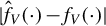 $|\hat {f}_V(\cdot )-f_V(\cdot )|$
. The result of
$|\hat {f}_V(\cdot )-f_V(\cdot )|$
. The result of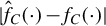 $|\hat {f}_C(\cdot )-f_C(\cdot )|$
can be shown in a similar way and is therefore omitted.
$|\hat {f}_C(\cdot )-f_C(\cdot )|$
can be shown in a similar way and is therefore omitted.
Let $\mathscr {C}_V$
be a closed inner subset of
$\mathscr {C}_V$
be a closed inner subset of $[\underline {v},\overline {v}]$
, and
$[\underline {v},\overline {v}]$
, and $\tilde {f}_V(\cdot )$
be the (infeasible) one-step local linear density estimator (i.e.,
$\tilde {f}_V(\cdot )$
be the (infeasible) one-step local linear density estimator (i.e., $p=1$
) which uses the unobserved true private values
$p=1$
) which uses the unobserved true private values $V_i$
instead of
$V_i$
instead of $\hat {V}_i$
. According to Lemma 6, we can show that
$\hat {V}_i$
. According to Lemma 6, we can show that $\sup _{v\in [\underline v, \overline v]}|\tilde {f}_V(v)-f_V(v)|=O_p\left ((\log n/n)^{1/5}\right )$
given a bandwidth
$\sup _{v\in [\underline v, \overline v]}|\tilde {f}_V(v)-f_V(v)|=O_p\left ((\log n/n)^{1/5}\right )$
given a bandwidth $h_V = \lambda _V(\log n/n)^{1/5}$
. Since
$h_V = \lambda _V(\log n/n)^{1/5}$
. Since $\hat {f}_V(v)-f_V(v)=[\hat {f}_V(v)-\tilde {f}_V(v)]+[\tilde {f}_V(v)-f_V(v)]$
, it remains to show that
$\hat {f}_V(v)-f_V(v)=[\hat {f}_V(v)-\tilde {f}_V(v)]+[\tilde {f}_V(v)-f_V(v)]$
, it remains to show that $\sup _{v\in \mathscr {C}_V} \big | \hat {f}_V(v)-\tilde {f}_V(v)\big | = O_p \big ((\log n/n)^{1/5}\big )$
.
$\sup _{v\in \mathscr {C}_V} \big | \hat {f}_V(v)-\tilde {f}_V(v)\big | = O_p \big ((\log n/n)^{1/5}\big )$
.
Let $\mathscr {C}^{\prime }_V=\bigcup _{v\in \mathscr {C}_V}[v-\Delta ,v+\Delta ]$
and
$\mathscr {C}^{\prime }_V=\bigcup _{v\in \mathscr {C}_V}[v-\Delta ,v+\Delta ]$
and $\mathscr {C}^{\prime \prime }_V=\bigcup _{v\in \mathscr {C}^{\prime }_V}[v-\Delta ,v+\Delta ]$
for some
$\mathscr {C}^{\prime \prime }_V=\bigcup _{v\in \mathscr {C}^{\prime }_V}[v-\Delta ,v+\Delta ]$
for some $\Delta>0$
. By construction,
$\Delta>0$
. By construction, $\mathscr {C}^{\prime }_V$
and
$\mathscr {C}^{\prime }_V$
and $\mathscr {C}^{\prime \prime }_V$
are also closed, and
$\mathscr {C}^{\prime \prime }_V$
are also closed, and $\mathscr {C}_V\subset \mathscr {C}^{\prime }_V\subset \mathscr {C}^{\prime \prime }_V$
. Since
$\mathscr {C}_V\subset \mathscr {C}^{\prime }_V\subset \mathscr {C}^{\prime \prime }_V$
. Since $\mathscr {C}_V$
is a closed inner subset of
$\mathscr {C}_V$
is a closed inner subset of $[\underline {v},\overline {v}]$
,
$[\underline {v},\overline {v}]$
, $\Delta $
can be chosen small enough such that
$\Delta $
can be chosen small enough such that $\mathscr {C}^{\prime \prime }_V\subset [\underline {v},\overline {v}]$
. Now, by part (ii) of Lemma 5, for
$\mathscr {C}^{\prime \prime }_V\subset [\underline {v},\overline {v}]$
. Now, by part (ii) of Lemma 5, for $v\in \mathscr {C}_V$
and n large enough,
$v\in \mathscr {C}_V$
and n large enough, $\hat {f}_V(v)$
uses at most observations
$\hat {f}_V(v)$
uses at most observations $\hat {V}_i$
in
$\hat {V}_i$
in $\mathscr {C}^{\prime }_V$
and for which
$\mathscr {C}^{\prime }_V$
and for which $V_i$
is in
$V_i$
is in $\mathscr {C}^{\prime \prime }_V$
. Because (i) for any
$\mathscr {C}^{\prime \prime }_V$
. Because (i) for any $v\in \mathscr {C}_V$
,
$v\in \mathscr {C}_V$
, $\tilde {f}_V(v)$
uses at most
$\tilde {f}_V(v)$
uses at most $V_i$
in
$V_i$
in $\mathscr {C}^{\prime \prime }_V$
and (ii) both
$\mathscr {C}^{\prime \prime }_V$
and (ii) both $\hat {f}_V(v)$
and
$\hat {f}_V(v)$
and $\tilde {f}_V(v)$
are first-order asymptotically equivalent (in convergence rate) to the standard kernel density estimator, we can then obtain the convergence rate by analyzing the latter as follows:
$\tilde {f}_V(v)$
are first-order asymptotically equivalent (in convergence rate) to the standard kernel density estimator, we can then obtain the convergence rate by analyzing the latter as follows:
 $$\begin{align*}\hat{f}_V(v)-\tilde{f}_V(v) = \frac{1}{nh_V}\sum_{i=1}^n \mathbb{1}(V_i\in\mathscr{C}^{\prime\prime}_V)\big[K_V\big(\frac{v-\hat{V}_i}{h_V}\big)-K_V\big(\frac{v-V_i}{h_V}\big)\big].\end{align*}$$
A second-order Taylor expansion gives the following:
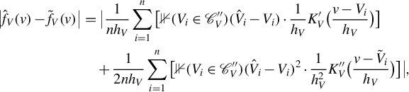 $$ \begin{align*} \big|\hat{f}_V(v)-\tilde{f}_V(v)\big| &= \big|\frac{1}{nh_V}\sum_{i=1}^n\big[\mathbb{1}(V_i\in\mathscr{C}^{\prime\prime}_V)(\hat{V}_i-V_i)\cdot\frac{1}{h_V}K^{\prime}_V\big( \frac{v-V_i}{h_V}\big)\big]\\& \quad +\frac{1}{2nh_V}\sum_{i=1}^n\big[\mathbb{1}(V_i\in\mathscr{C}^{\prime\prime}_V)(\hat{V}_i-V_i)^2\cdot\frac{1}{h_V^2}K^{\prime\prime}_V \big(\frac{v-\tilde{V}_i}{h_V}\big)\big]\big|, \end{align*} $$
where $\tilde {V}_i$
is some point between
$\tilde {V}_i$
is some point between $\hat {V}_i$
and
$\hat {V}_i$
and $V_i$
. By triangular inequality,
$V_i$
. By triangular inequality,
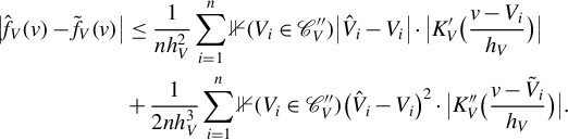 $$ \begin{align} \big|\hat{f}_V(v)-\tilde{f}_V(v)\big|&\leq \frac{1}{nh_V^2}\sum_{i=1}^n \mathbb{1}(V_i\in\mathscr{C}^{\prime\prime}_V)\big|\hat{V}_i-V_i\big|\cdot\big|K^{\prime}_V\big( \frac{v-V_i}{h_V}\big)\big| \nonumber\\ &+ \frac{1}{2nh_V^3}\sum_{i=1}^n \mathbb{1}(V_i\in\mathscr{C}^{\prime\prime}_V)\big(\hat{V}_i-V_i\big)^2\cdot\big|K^{\prime\prime}_V\big( \frac{v-\tilde{V}_i}{h_V}\big)\big|. \end{align} $$
Because $\left |K^{\prime \prime }_V\left (\frac {v-\tilde {V}_i}{h_V}\right )\right |\leq \sup _u |K^{\prime \prime }_V(u)|$
, the right-hand side of (A.18) is bounded by
$\left |K^{\prime \prime }_V\left (\frac {v-\tilde {V}_i}{h_V}\right )\right |\leq \sup _u |K^{\prime \prime }_V(u)|$
, the right-hand side of (A.18) is bounded by
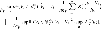 $$\begin{align*} &\frac{1}{h_V}\sup_i \mathbb{1}(V_i\in\mathscr{C}^{\prime\prime}_V)\big|\hat{V}_i-V_i\big|\cdot\frac{1}{nh_V}\sum_{i=1}^n \big| K^{\prime}_V\big( \frac{v-V_i}{h_V} \big) \nonumber \\ &\quad \big|+\frac{1}{2h_V^3}\sup_i \mathbb{1}(V_i\in\mathscr{C}^{\prime\prime}_V)\big|\hat{V}_i-V_i\big|^2\cdot \sup_u |K^{\prime\prime}_V(u)|.\end{align*}$$
By part (ii) of Lemma 5 and Assumption G,
 $$ \begin{align} &\big|\hat{f}_V(v)-\tilde{f}_V(v)\big| \nonumber\\ &\leq O_p\big((\log n / n)^{1/5}\big)\cdot\frac{1}{nh_V} \sum_{i=1}^n \big| K^{\prime}_V\big( \frac{v-V_i}{h_V} \big)\big|+O_p\big( (\log n / n)^{1/5}\big)\cdot\sup_u|K^{\prime\prime}_V(u)|. \end{align} $$
It can be shown that $\frac {1}{nh_V}\sum _{i=1}^n \big | K^{\prime }_V\big ( \frac {v-V_i}{h_V} \big )\big |$
converges uniformly to
$\frac {1}{nh_V}\sum _{i=1}^n \big | K^{\prime }_V\big ( \frac {v-V_i}{h_V} \big )\big |$
converges uniformly to $f_V(v)\int _{-\infty }^\infty |K^{\prime }_V(u)|\,\mathrm {d} u$
thus being bounded uniformly. Moreover,
$f_V(v)\int _{-\infty }^\infty |K^{\prime }_V(u)|\,\mathrm {d} u$
thus being bounded uniformly. Moreover, $\sup _u|K^{\prime \prime }_V(u)|<\infty $
by Assumption F. Then it follows that
$\sup _u|K^{\prime \prime }_V(u)|<\infty $
by Assumption F. Then it follows that $\sup _{v\in \mathscr {C}_V}|\hat {f}_V(v)-\tilde {f}_V(v)|=O_p\big ((\log n/n)^{1/5}\big )$
. The desired conclusion therefore follows.
$\sup _{v\in \mathscr {C}_V}|\hat {f}_V(v)-\tilde {f}_V(v)|=O_p\big ((\log n/n)^{1/5}\big )$
. The desired conclusion therefore follows.
A.12 Auxiliary Lemmas
We first define the local polynomial density estimator as given in Section 4.1. For a given random sample of $\{Z_1,Z_2,\dots ,Z_m\}$
from a distribution with a density of
$\{Z_1,Z_2,\dots ,Z_m\}$
from a distribution with a density of $g_Z(\cdot )$
on
$g_Z(\cdot )$
on $[\underline z,\overline z]$
, the boundary-adaptive local polynomial density estimator (with a polynomial of order p) is defined as
$[\underline z,\overline z]$
, the boundary-adaptive local polynomial density estimator (with a polynomial of order p) is defined as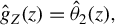 $\hat g_Z(z) = \hat {\theta }_2(z),$
where
$\hat g_Z(z) = \hat {\theta }_2(z),$
where $\hat \theta (z) = \text {argmin}_{\theta \in \mathbb {R}^{p+1}} \sum _{i=1}^m \big [ \hat {G}_Z(Z_i) - \theta _1 - \theta _2\cdot (Z_i-z) - \dots - \theta _{p+1}\cdot (Z_i-z)^p \big ]^2\cdot K\big ((Z_i-z)/h\big )$
with
$\hat \theta (z) = \text {argmin}_{\theta \in \mathbb {R}^{p+1}} \sum _{i=1}^m \big [ \hat {G}_Z(Z_i) - \theta _1 - \theta _2\cdot (Z_i-z) - \dots - \theta _{p+1}\cdot (Z_i-z)^p \big ]^2\cdot K\big ((Z_i-z)/h\big )$
with $\hat G_Z(z) = (1/m)\sum _{i=1}^m \mathbf {1} (Z_i\leq z)$
,
$\hat G_Z(z) = (1/m)\sum _{i=1}^m \mathbf {1} (Z_i\leq z)$
, $K(\cdot )$
being a kernel function and h being a bandwidth. The following lemma characterizes the uniform convergence rate of
$K(\cdot )$
being a kernel function and h being a bandwidth. The following lemma characterizes the uniform convergence rate of $\hat g_Z(\cdot )$
on
$\hat g_Z(\cdot )$
on $[\underline z,\overline z]$
. It is a corollary of Theorem 1 in Cattaneo et al. (Reference Cattaneo, Chandak, Jansson and Ma2023) when there is no conditional covariate.
$[\underline z,\overline z]$
. It is a corollary of Theorem 1 in Cattaneo et al. (Reference Cattaneo, Chandak, Jansson and Ma2023) when there is no conditional covariate.
Lemma 6. Suppose that (i) the density $g_Z(\cdot )$
is p-th continuously differentiable and bounded away from zero on
$g_Z(\cdot )$
is p-th continuously differentiable and bounded away from zero on $[\underline z,\overline z]$
, (ii) the symmetric kernel
$[\underline z,\overline z]$
, (ii) the symmetric kernel $K(\cdot )$
is nonnegative on a support of
$K(\cdot )$
is nonnegative on a support of $[-1,1]$
and satisfies
$[-1,1]$
and satisfies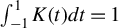 $\int _{-1}^1 K(t) dt =1$
and
$\int _{-1}^1 K(t) dt =1$
and $\vert K(t) - K(s) \vert \leq L\cdot \vert t - s \vert $
for some
$\vert K(t) - K(s) \vert \leq L\cdot \vert t - s \vert $
for some $L>0$
, and (iii) the bandwidth
$L>0$
, and (iii) the bandwidth $h \rightarrow 0$
and
$h \rightarrow 0$
and $log(n)/(nh) \rightarrow 0 $
. Then
$log(n)/(nh) \rightarrow 0 $
. Then $\sup _{z\in [\underline z,\overline z]} \big \vert \hat g_Z(z) - g_Z(z) \big \vert = O_p \big ( h^p + \sqrt {log(n)/ (nh)} \big )$
.
$\sup _{z\in [\underline z,\overline z]} \big \vert \hat g_Z(z) - g_Z(z) \big \vert = O_p \big ( h^p + \sqrt {log(n)/ (nh)} \big )$
.
Proof. Our local polynomial density estimator (for unconditional density) can be viewed as a special case of the Cattaneo et al.’s (Reference Cattaneo, Chandak, Jansson and Ma2023) local polynomial one for conditional density, namely, $\mathfrak {p} = p$
,
$\mathfrak {p} = p$
, $\vartheta = 0$
,
$\vartheta = 0$
, $d=0$
, and
$d=0$
, and $\hat F(y_i|\mathbf {x})$
being replaced by the empirical CDF
$\hat F(y_i|\mathbf {x})$
being replaced by the empirical CDF $\hat F(y_i) = (1/n)\sum _{j=1}^n \mathbf {1}(y_j \leq y_i)$
in their case.
$\hat F(y_i) = (1/n)\sum _{j=1}^n \mathbf {1}(y_j \leq y_i)$
in their case.
We can then follow the technique used in the proofs of their Lemma 1 and Theorem 1 (i.e., discretization, union bound, and Bernstein’s inequality), and establish that
 $$ \begin{align*} \sup_{z\in[\underline z,\overline z]} \big\vert \hat g_Z(z) - g_Z(z) \big\vert = O_p \Big( h^p + \sqrt{log(n)/ (nh)} \Big).\\[-41pt] \end{align*} $$
The second auxiliary lemma is about the convergence rates of $\hat g_S(\cdot )$
and
$\hat g_S(\cdot )$
and $\hat g_B(\cdot )$
on the interval of
$\hat g_B(\cdot )$
on the interval of $[\underline s,\overline b]$
.
$[\underline s,\overline b]$
.
Lemma 7. Under Assumptions A and E–G, there are (i) $\sup _{s\in [\underline s,\overline b]} \big \vert \hat g_S(s) - g_S(s) \big \vert = O_p \big ( h_S^2 + \sqrt {log(n)/ (nh_S)} \big )$
and (ii)
$\sup _{s\in [\underline s,\overline b]} \big \vert \hat g_S(s) - g_S(s) \big \vert = O_p \big ( h_S^2 + \sqrt {log(n)/ (nh_S)} \big )$
and (ii) $\sup _{b\in [\underline s,\overline b]} \big \vert \hat g_B(b) - g_B(b) \big \vert = O_p \big ( h_B^2 + \sqrt {log(n)/ (nh_B)} \big )$
.
$\sup _{b\in [\underline s,\overline b]} \big \vert \hat g_B(b) - g_B(b) \big \vert = O_p \big ( h_B^2 + \sqrt {log(n)/ (nh_B)} \big )$
.
Proof. We only show part (i). Part (ii) can be shown similarly, and is therefore omitted. Consider an infeasible estimator $\tilde g_S$
that uses the true
$\tilde g_S$
that uses the true $\overline b$
instead of its estimator
$\overline b$
instead of its estimator $\hat {\overline b}$
to define the subsample as
$\hat {\overline b}$
to define the subsample as $\{S_i:S_i\leq \overline b\}$
with size of
$\{S_i:S_i\leq \overline b\}$
with size of $\tilde {n}^-_S$
. Thus,
$\tilde {n}^-_S$
. Thus,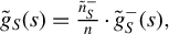 $\tilde g_S(s) = \frac {\tilde {n}^-_S}{n}\cdot \tilde {g}_S^-(s),$
where
$\tilde g_S(s) = \frac {\tilde {n}^-_S}{n}\cdot \tilde {g}_S^-(s),$
where $\tilde {g}_S^-(\cdot )$
is a local quadratic density estimator (i.e.,
$\tilde {g}_S^-(\cdot )$
is a local quadratic density estimator (i.e., $p=2$
) from the subsample of
$p=2$
) from the subsample of $\{S_i: S_i\leq \overline b\}$
. By Lemma 6, the convergence rate of
$\{S_i: S_i\leq \overline b\}$
. By Lemma 6, the convergence rate of $\tilde g_S^-(\cdot )$
on
$\tilde g_S^-(\cdot )$
on $[\underline s,\overline b]$
is given by
$[\underline s,\overline b]$
is given by
 $$ \begin{align*} \sup_{s\in[\underline s, \overline b]} \vert \tilde g_S^-(s) - g_S^-(s) \vert = O_p\Big(h_S^2 + \sqrt{log(n)/ (nh_S)}\Big), \end{align*} $$
where $g_S^-(\cdot )$
is the conditional density of sellers’ bids conditional on
$g_S^-(\cdot )$
is the conditional density of sellers’ bids conditional on $S\leq \overline b$
, that is,
$S\leq \overline b$
, that is, $g_S^-(s) = g_S(s) / G_S(\overline b)$
for any
$g_S^-(s) = g_S(s) / G_S(\overline b)$
for any $s\in [\underline s,\overline b]$
. This implies that
$s\in [\underline s,\overline b]$
. This implies that
 $$ \begin{align} \sup_{s\in[\underline s, \overline b]} \vert \tilde g_S(s) - g_S(s) \vert = \sup_{s\in[\underline s, \overline b]} \Big\vert \frac{\tilde{n}^-_S}{n}\cdot \tilde g_S^-(s) - G_S(\overline b)\cdot g_S^-(s) \Big\vert = O_p\Big(h_S^2 + \sqrt{log(n)/ (nh_S)}\Big), \end{align} $$
where $ \big \vert \frac {\tilde {n}^-_S}{n} - G_S(\overline b)\big \vert = \big \vert \hat G_S(\overline b) - G_S(\overline b)\big \vert = O_p\big (log(n)/\sqrt {n}\big )$
with
$ \big \vert \frac {\tilde {n}^-_S}{n} - G_S(\overline b)\big \vert = \big \vert \hat G_S(\overline b) - G_S(\overline b)\big \vert = O_p\big (log(n)/\sqrt {n}\big )$
with $\hat G_S(\cdot )$
being the empirical CDF of sellers’ bids.
$\hat G_S(\cdot )$
being the empirical CDF of sellers’ bids.
We next study the difference between $\hat g_S$
and
$\hat g_S$
and $\tilde g_S$
. It involves two differences:
$\tilde g_S$
. It involves two differences: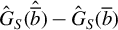 $\hat G_S(\hat {\overline b}) - \hat {G}_S(\overline b)$
and
$\hat G_S(\hat {\overline b}) - \hat {G}_S(\overline b)$
and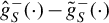 $\hat g_S^-(\cdot ) - \tilde g_S^-(\cdot )$
. The first difference can be characterized as follows:
$\hat g_S^-(\cdot ) - \tilde g_S^-(\cdot )$
. The first difference can be characterized as follows:
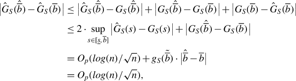 $$ \begin{align} \big\vert\hat G_S(\hat{\overline b}) - \hat{G}_S(\overline b)\big\vert & \leq \big\vert\hat G_S(\hat{\overline b}) - G_S(\hat{\overline b})\big\vert + \big\vert G_S(\hat{\overline b}) - G_S(\overline b)\big\vert + \big\vert G_S(\overline b) - \hat{G}_S(\overline b)\big\vert\nonumber\\ &\leq 2\cdot \sup_{s\in [\underline s,\overline b] } \big\vert \hat G_S(s) - G_S(s)\big\vert + \big\vert G_S(\hat{\overline b}) - G_S(\overline b)\big\vert \nonumber\\ & = O_p (log(n)/\sqrt{n}) + g_S(\tilde {\overline b})\cdot\big\vert \hat{\overline b} - \overline b\big\vert\nonumber \\ & = O_p (log(n)/\sqrt{n}), \end{align} $$
where $\tilde {\overline b} \in [\hat {\overline b}, \overline b]$
, the first equality holds due to
$\tilde {\overline b} \in [\hat {\overline b}, \overline b]$
, the first equality holds due to $\sup _{s\in [\underline s,\overline b] } \big \vert \hat G_S(s) - G_S(s)\big \vert = O_p (log(n)/\sqrt {n})$
and Taylor expansion, and the second equality is derived by
$\sup _{s\in [\underline s,\overline b] } \big \vert \hat G_S(s) - G_S(s)\big \vert = O_p (log(n)/\sqrt {n})$
and Taylor expansion, and the second equality is derived by $\sup _{s\in [\underline s,\overline b]} g_S(s) \leq \overline {g}_S$
and
$\sup _{s\in [\underline s,\overline b]} g_S(s) \leq \overline {g}_S$
and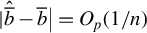 $\vert \hat {\overline b} - \overline b\big \vert = O_p(1/n)$
. In addition, the second difference is given by
$\vert \hat {\overline b} - \overline b\big \vert = O_p(1/n)$
. In addition, the second difference is given by
 $$ \begin{align} \sup_{s\in[\underline s,\overline b]}\big\vert\hat g_S^-(s) - \tilde g_S^-(s)\big\vert = \sup_{s\in[\hat{\overline b} - h_S,\overline b]}\big\vert\hat g_S^-(s) - \tilde g_S^-(s)\big\vert = o_p\Big(h_S^2 + \sqrt{log(n)/ (nh_S)}\Big), \end{align} $$
where the first equality holds because of $\hat g_S^-(s) = \tilde g_S^-(s)$
for all
$\hat g_S^-(s) = \tilde g_S^-(s)$
for all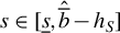 $s\in [\underline s,\hat {\overline b} - h_S]$
, and the second equality is obtained due to three facts: (i) there is a uniform convergence of the criterion functions used for obtaining the density estimators, which can be written as
$s\in [\underline s,\hat {\overline b} - h_S]$
, and the second equality is obtained due to three facts: (i) there is a uniform convergence of the criterion functions used for obtaining the density estimators, which can be written as
 $$ \begin{align*}\hat{Q}(s) = \frac{1}{n}\sum_{i=1}^n\big[ \hat{G}_S (S_i) - \theta_1 - \theta_2\cdot(S_i-s) - \theta_3(S_i-s)^2 \big]^2\cdot\mathbb{1} (S_i\leq \hat{\overline{b}}) \cdot K(\frac{S_i-s}{h_s})\end{align*} $$
for estimating $\hat {g}_S^-(s)$
, and
$\hat {g}_S^-(s)$
, and
 $$ \begin{align*}\tilde{Q}(s) = \frac{1}{n}\sum_{i=1}^n\big[ \tilde{G}_S (S_i) - \theta_1 - \theta_2\cdot(S_i-s) - \theta_3(S_i-s)^2 \big]^2\cdot\mathbb{1} (S_i\leq \overline{b}) \cdot K(\frac{S_i-s}{h_s})\end{align*} $$
for estimating $\tilde {g}_S^-(s)$
with
$\tilde {g}_S^-(s)$
with $\hat { G}_S(s) = (1/n)\cdot \sum _{i=1}^n \mathbb {1} (S_i\leq s)\cdot \mathbb {1}(S_i\leq \hat {\overline {b} }) $
and
$\hat { G}_S(s) = (1/n)\cdot \sum _{i=1}^n \mathbb {1} (S_i\leq s)\cdot \mathbb {1}(S_i\leq \hat {\overline {b} }) $
and $\tilde {G}_S(s)= (1/n)\cdot \sum _{i=1}^n \mathbb {1} (S_i\leq s)\cdot \mathbb {1}(S_i\leq \overline {b} )$
; (ii)
$\tilde {G}_S(s)= (1/n)\cdot \sum _{i=1}^n \mathbb {1} (S_i\leq s)\cdot \mathbb {1}(S_i\leq \overline {b} )$
; (ii) $\hat {g}_S^-(s)$
for any
$\hat {g}_S^-(s)$
for any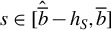 $s\in [\hat {\overline b} - h_S,\overline b]$
uses all data in the interval of
$s\in [\hat {\overline b} - h_S,\overline b]$
uses all data in the interval of $[s-h_S,\hat {\overline b}]$
which consists of a rough fraction no less than
$[s-h_S,\hat {\overline b}]$
which consists of a rough fraction no less than $G_S(\hat {\overline b}) - G_S(\overline b - h_S) = O_p(h_S)$
in the whole sample; and (iii)
$G_S(\hat {\overline b}) - G_S(\overline b - h_S) = O_p(h_S)$
in the whole sample; and (iii) $\tilde {g}_S^-(s)$
for any
$\tilde {g}_S^-(s)$
for any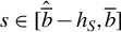 $s\in [\hat {\overline b} - h_S,\overline b]$
uses all data in the interval of
$s\in [\hat {\overline b} - h_S,\overline b]$
uses all data in the interval of $[s-h_S,\overline b]$
, namely, uses some additional observations (relative to
$[s-h_S,\overline b]$
, namely, uses some additional observations (relative to $\hat {g}_S^-(s)$
) with a rough fraction no more than
$\hat {g}_S^-(s)$
) with a rough fraction no more than $G_S(\overline b) - G_S(\hat {\overline b}) = O_p(1/n)$
in the whole sample.
$G_S(\overline b) - G_S(\hat {\overline b}) = O_p(1/n)$
in the whole sample.
Therefore, the difference between $\hat g_S$
and
$\hat g_S$
and $\tilde g_S$
can be bounded as
$\tilde g_S$
can be bounded as
 $$ \begin{align} \sup_{s\in[\underline s,\overline b]} \big\vert \hat g_S(s) - \tilde g_S(s)\big\vert = \sup_{s\in[\underline s,\overline b]} \big\vert \hat G_S(\hat{\overline b})\cdot\hat g_S^-(s) - \hat G_S(\overline b)\cdot \tilde{g}_S^-(s)\big\vert = o_p\Big(h_S^2 + \sqrt{log(n)/ (nh_S)}\Big), \end{align} $$
where the second equality comes from (A.21) and (A.22).
In summary, we have
 $$ \begin{align*} \sup_{s\in[\underline s,\overline b]} \big\vert \hat g_S(s) - g_S(s)\big\vert &\leq \sup_{s\in[\underline s,\overline b]} \big\vert \hat g_S(s) - \tilde{g}_S(s)\big\vert + \sup_{s\in[\underline s,\overline b]} \big\vert \tilde g_S(s) - g_S(s)\big\vert \\ &= O_p\Big(h_S^2 + \sqrt{log(n)/ (nh_S)}\Big), \end{align*} $$
where the last equality comes from (A.20) and (A.23). The desired conclusion therefore follows.
COMPETING INTEREST STATEMENT
The authors declare that no competing interests exist.
FUNDING STATEMENT
This work was supported by the Fundamental Research Funds for the Central Universities, China, under Grant Number 20720251031, and the National Natural Science Foundation of China under Grant Number 72394392.
SUPPLEMENTARY MATERIAL
The supplementary material for this article can be found at https://doi.org/10.1017/S0266466626100413.








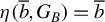






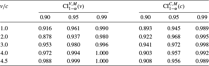


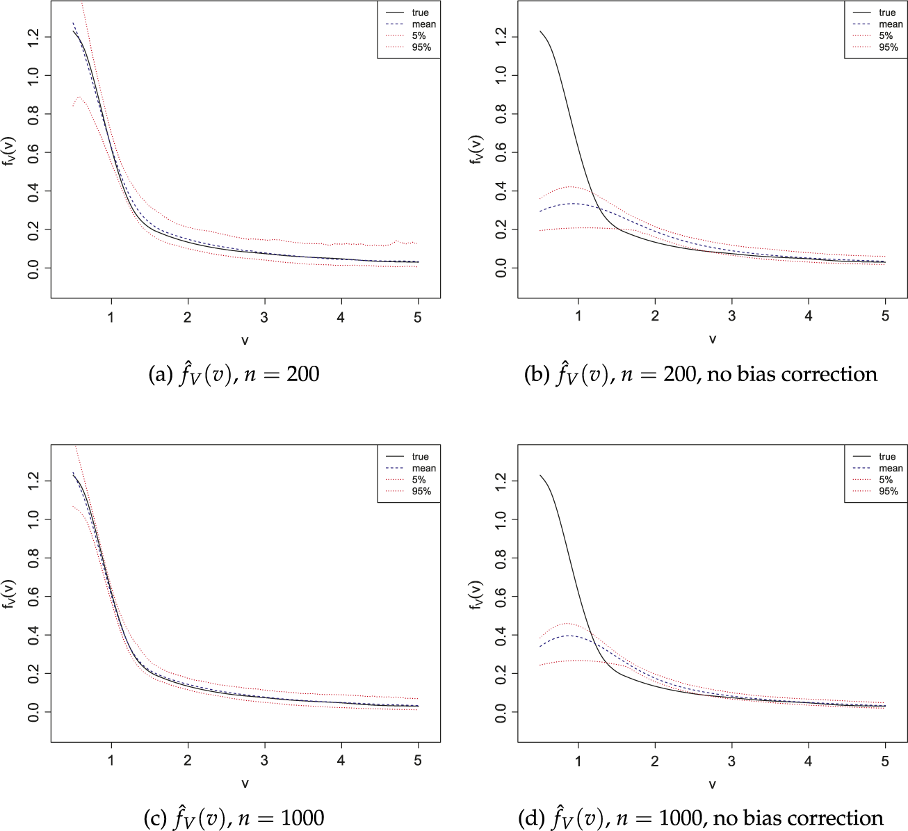


 Open access

