


Introduction
During the past decade several authors have used the finite-element technique to model numerically the flow of an ice mass; Reference NguyenNguyen (unpublished), Reference SchmidtSchmidt (1977), Reference IkenIken (1977, Reference Iken1981), Reference Hooke, Hooke, Raymond, Hotchkiss and GustafsonHooke and others (1979), Reference Emery, Emery, Hanafy, Holdsworth and MirzaEmery and others (1979), Reference MacAyeal and ThomasMacAyeal and Thomas (1982, Reference MacAyeal and Thomas1984), Reference SikoniaSikonia (1982), Reference Fastook and SchmidtFastook and Schmidt (1982), Reference EchelmeyerEchelmeyer (1983), and Reference RaymondRaymond (1983). Applications have ranged from the overall motion of the Ross Ice Shelf (Reference MacAyeal and ThomasMacAyeal and Thomas, 1982, Reference MacAyeal and Thomas1984) to the development of a crack near an ice cliff (Reference IkenIken, 1977), and from a fast-moving, calving temperate glacier (Reference SikoniaSikonia, 1982) to a slow-moving, cold ice cap (Reference Hooke, Hooke, Raymond, Hotchkiss and GustafsonHooke and others, 1979).
The method is thus well established as a powerful tool to analyze many different topics in ice dynamics. Much of the reason for this popularity lies in its ability to handle boundary conditions easily, in particular, the complex geometric shapes of typical ice masses in the real world. It also lends itself to a modular programming approach, which makes it readily adaptable to different situations.
None of the published works, however, addresses specifically the time-dependent modeling of an arbitrarily shaped ice mass. Such generality, at least for plane (“two-dimensional”) flow, was one of two primary objectives of this paper. The other was to develop procedures to allow the model to be used by someone who had only a cursory knowledge of the details of the method, and to require, as much as possible, only glaciological data as input. These objectives were achieved and the resulting software will be described extensively in a forthcoming open-file report of the U.S. Geological Survey. This will make a reasonably general finite-element ice-flow model available to the glaciologist who has neither the time nor the inclination to commit himself to a long and often frustrating development period.
This model is based on an earlier one used by Reference SikoniaSikonia (1982) on the lowermost section of Columbia Glacier, Alaska. Numerous minor improvements were made to achieve the above objectives but only the two major ones will be described here: modeling of a “typical” glacier end, where the ice thickness tends to zero, and an automatic procedure for generating an appropriate “mesh” of “finite elements” for approximating the specified geometry. Neither of these features appears in previous works but their inclusion enables analysis of different problems to be done without any program modification or extensive data preparations.
The Finite-Element Method
A disadvantage of the finite-element method is that it is conceptually more difficult to understand than its finite-difference counterpart for solving differential equations. A description detailed enough to give a working knowledge of the method covers many chapters in a book and is beyond the scope of this paper. Many text-books describe the method in ample detail, for example, Reference ZienkiewiczZienkiewicz (1977) or Reference Lapidus and PinderLapidus and Pinder (1982). Nevertheless, a brief description of the method and its terminology is given to serve both as a basis for subsequent discussions and as a partial review of the subject for the glaciological literature, which has not been done previously.
The region of interest is subdivided into a set of discrete sub-regions, called “finite elements”, and the unknown functions, u(xi ), are approximated within each element by some linear combination of interpolating polynomials, fj (xi ), referred to as “shape” or “basis” functions:

where xi represents the spatial coordinates and the Uj are coefficients to be determined. The degree of these basis functions is specified, based on the desired physical size of the elements and upon some a priori knowledge of how the functions are likely to vary within each element.
A set of N points (or “nodes”) is then chosen within each element and the basis functions selected so that function f j has a value of one at node j, and a value of zero at all other nodes. When this is done, U j becomes the value of the unknown function at that node. The number and distribution of the nodes are dictated by the maximum degree of the basis functions chosen. Since polynomials are used, all derivatives in the original differential equations are now easily evaluated when Equation (1) is substituted for the unknown functions.
By utilizing a method of “weighted residuals”, the differential equations can be converted to a set of linear simultaneous equations, one for each unknown coefficient U j , which can then be solved using standard methods. In the process, the differential equations are changed to an integral form, with the integrations performed over the entire domain of the element (or along its surface for boundary conditions). The solution obtained thus approximates the true one in an integral sense over each element, rather than only at discrete points as in a finite-difference formulation. This implies that the elements can be made bigger, that is, more “finite”, and thus hopefully fewer nodes are required for an adequate solution to the problem.
Furthermore, since an integral over a region is equal to the sum of integrals over a set of sub-regions, the equations for all elements can be combined into a “global” set of linear simultaneous equations. Although this results in a large number of unknowns and equations (hundreds or thousands), the solution for the entire ice mass can still be obtained with standard methods for such equations.
Basis functions are also used to handle curvilinear element shapes rather than being restricted to purely rectangular ones. This model utilizes “isoparametric” elements, in which basis functions of the same degree are used for both the unknown function interpolation and the coordinate transformation (Reference ZienkiewiczZienkiewiez, 1977).
The heart of the finite-element method is the basis functions. They specify how the functional variation across the element is to be approximated. The reader is cautioned to keep Equation (1) in mind and not to interpret a basis function directly as a “conventional” interpolating polynomial. This is particularly true for two-dimensional basis functions (which are used here); these are formed by combining basis functions defined separately for the two coordinate directions. This allows “mixed-order” basis functions to be used, for example, linear in one direction but quadratic in the other. In fact, the order can be different along opposite edges of an element, which allows a transition to be made, if desired, between different degrees of functional variation.
The basis functions are also defined separately for each unknown function. Thus, by varying the number and distribution of nodes in an element and, whether or not a particular function is assigned to a particular node, many complex physical situations can be simulated. In addition, the elements and nodes can be distributed non-uniformly over the entire region of interest so that the calculations can be concentrated where the unknowns are varying more rapidly.
Another advantage of the particular manner in which basis functions are developed is that it is possible to write computer code which can automatically select different orders of basis functions, depending upon the input (Reference Taylor and ZienkiewiczTaylor, 1977). The model does not have to be tied rigidly to any particular type; the one described here, in fact, can alternate between various basis functions by changing a single input variable.
Application to Ice Flow
The particular formulation of the method applicable to the flow of viscous materials has been given by Reference ZienkiewiczZienkiewiez (1977), and the adaptation of this for ice flow that is used here has been given by Reference SikoniaSikonia (1982). Velocity and pressure are treated as the dependent variables; pressure must be added because in a fluid the deformation rates are related only to the deviatoric stresses and so the pressure term is necessary to complete the stress solution.
Field equations
The governing differential equations are those of conservation of momentum,
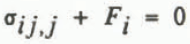
where σ ij is the stress tensor, Fi are the body forces, a comma denotes differentiation and a repeated index implies summation over that index; and conservation of mass,
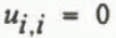
where ui now refers only to the velocity unknowns. The indices i, j range over the different spatial coordinates used (a total of two in this model). The body forces are simply those imposed by gravity:
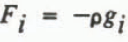
where ρ is the ice density and gi the acceleration of gravity. Equation (2) assumes that ice flows by creep and that inertial effects are negligible; Equation (3) assumes that ice is incompressible. These are realistic simplifications and any approximation that they introduce is undoubtedly insignificant relative to other uncertainties.
The constitutive relationship between stress and deformation rate that is used in the model is the usual Glen’s flow law:
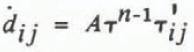
where


τ is the effective shear stress, defined as

A and n are constants which are specified, δ ij is the Kronecker delta, and p is the pressure, defined as

This is the usual starting point for most ice-flow analyses, either analytical or numerical (Reference Raymond and ColbeckRaymond, 1980; Reference PatersonPaterson, [c1981]). The effective shear stress τ is a function of all the shear-stress components and thus introduces a non-linearity into the problem. This is incorporated into the calculations using the iterative Newton-Raphson method.
Approximations
The only significant approximation made so far is the one which assumes that Glen’s flow law is, in fact, the true constitutive relation. The parameters A and n can be fixed constants for the entire ice mass or they can be prescribed as known functions of the spatial coordinates if desired. The singularity exhibited by such a flow law, where viscosity becomes infinite as the stress approaches zero at the ice surface (Reference HutterHutter, [c1983], p. 92), should not affect the model significantly since the Gaussian integration schemes never require evaluation of the flow law along any surfaces of the ice mass. Alternate flow laws, such as that suggested by Reference Smith and MorlandSmith and Morland (1981), could be added but it is not clear whether this would be worth the effort since the values of a flow law’s coefficients probably introduce a far greater uncertainty than does the form of the law itself.
Except for temperature and the approximations inherent in the finite-element technique itself, the only other approximation made is that the ice flow is planar, or “two-dimensional”. The model simulates the ice motion in a vertical section following some given flow line, and assumes this section is identical to all adjacent sections (in the transverse direction). A two-dimensional coordinate system, fixed in space, is assigned to this vertical section: X is horizontal, positive in the direction of flow, and Z is vertical, positive upward. With the plane-flow assumption, Equations (2) and (3) reduce to three equations in three unknowns: U, the X-component of velocity, W, the Z-component of velocity, and P, the pressure. Thus, given the geometry of the ice mass, the complete velocity and pressure distribution can be calculated.
Although the ice mass is assumed to be isothermal in this paper, this is not a mandatory restriction of the model. It can be made partially temperature-dependent if necessary. The ice temperature can be specified (as a function of Z, or of both X and Z) or it can be calculated at each iteration by using the steady-state temperature distribution derived by Reference RobinRobin (1955). Once the temperature at a point is known, it is used to adjust the parameter A in the flow law by using the Arrhenius relation (Reference PatersonPaterson, [C1981]). This can only be considered a rough approximation, however, since it only represents a steady-state decoupled solution.
No other approximations are made. Any physically reasonable surface and bed topography, for example, can be specified.
Time-dependency
This is introduced by allowing the upper surface of the ice to be a “free” surface. The velocity vectors along this surface are used to project the surface to a new position at a time Δt later. This gives a new ice-mass configuration, which is then solved as before for a new velocity distribution. The process is then repeated as often as necessary to simulate the time evolution of the ice mass. This simple explicit time-stepping technique can be used for any slow (creep) flow, where acceleration effects are negligible (Reference ZienkiewiczZienkiewiez, 1977). If the time interval is made too large, the solution will break down; in practice, however, typical desired intervals are well within this limit. Time is thus not directly an independent variable, since it is not necessary to do this for ice flow. The model is still referred to as “time-dependent”, however, even though the term “geometrically dynamic” (Reference SikoniaSikonia, 1982) is probably more appropriate.
Accumulation and ablation also affect the position of the ice surface. To incorporate their effects and perform the time-stepping, Reference SikoniaSikonia (1982) added a fourth unknown, the rate of change of thickness


where


Boundary conditions
The upper surface is assumed to be stress-free. The lower surface can be either sliding or not sliding. For the application described in this paper, the no-slip condition is used. In addition, an artificial boundary condition has to be added at the ends of the ice mass, because of the particular method by which these are modeled; this is detailed in a later section.
These boundary conditions are all that are needed to obtain stress, deformation rate, velocity, and pressure at a given time. When time-stepping is performed, the net balance

A sliding-boundary condition, although not used here, is also incorporated into the model. Since the shear stress and normal pressure at the bed are known quantities once the finite-element solution has been obtained, theories such as those of Reference WeertmanWeertman (1957), Reference BindschadlerBindschadler (1983), or Reference Morland, Morland, Smith and BoultonMorland and others (1984) can be used to calculate the sliding velocity. This is then applied as a boundary condition to the next iteration or time step. Alternatively, sliding can be simulated with a thin row of mesh elements along the base of the ice in which the parameter A in the flow law is artificially increased to produce a layer of lower viscosity (Reference SikoniaSikonia, 1982). In all cases, additional input data, such as bed roughness, water discharge, friction coefficient, or observed surface velocity, are required.
Basis functions
Following Reference SikoniaSikonia (1982), quadratic basis functions are used for all the unknowns, with the partial exception of the pressure, which is assumed to vary quadratically in the horizontal direction but only linearly in the vertical direction. Most, if not all, of the previous finite-element ice-flow models only utilize linear basis functions. Since this can be shown to resemble closely certain finite-difference formulations, at least for rectangular elements (Reference Lapidus and PinderLapidus and Pinder, 1982), the real power of the finite-element method is only realized when using higher-order basis functions. Quadratic basis functions can probably handle a wider range of ice-flow problems. Furthermore, since they are also used to approximate the bed and surface topography, more realistic configurations can be modeled.
This is a mixed-order interpolation scheme. Each element is a curvilinear quadrilateral with nine nodes, arranged in a 3 × 3 pattern. “Lagrangian” basis functions, formed from Lagrange polynomials, are used. Since pressure is always assumed to be linear vertically, the middle horizontal row of each element does not have a pressure unknown assigned to it. Globally, the nodes are arranged in vertical columns and curvilinear rows (Fig. 1).
The input data used for the modeling. The surface and bed topography each consist of about 70 points specified approximately uniformly in X. Cubic splines are used to interpolate in each data set. All other figures use the same scale and origin along both axes and so the axis labels are not shown on them. The solid dots and short dashed lines are the finite-element mesh generated by the algorithm described in the Appendix, for δ = 100%; thus the widest element column (the fifth from the left) is twice the width of the narrowest (the leftmost). This 10 x 2 element mesh is the one used for most of the other simulations in the other figures. Each element is a 9-node quadrilateral; the three nodes in each direction allow use of quadratic basis functions.

Computer code
The basic computer code used here is available in the literature: a general purpose program for finite-element analysis, coded in FORTRAN, has been given by Reference Taylor and ZienkiewiczTaylor (1977), and the modifications necessary for ice have been given by Reference SikoniaSikonia (1982).
Mesh Generation
A set of “mesh-generation” routines was developed to create automatically from glaciological data not only suitable coordinates for the mesh nodes but also the boundary conditions and all the other input required by the finite-element routines. The input data consist of the bed elevation, the surface elevation, and the balance rate. This is a significant improvement over earlier models in which such information must be generated manually. It simplifies enormously the preparation of the data for the program. It eliminates any human bias which might be introduced in deciding where to place the mesh nodes. Also, if the technique is suitably chosen, it can optimize, at least to some extent, the node distribution specifically for the analysis of ice flow, and can then maintain this optimization regardless of how the geometry of the ice mass changes with time.
To achieve this optimization, several methods were tried. Most were abandoned because they were not robust enough to work on a wide variety of surface and bed geometries. The one finally adopted is outlined in detail in (Figure 1) the Appendix. The X -coordinates of the nodes are determined by adjusting iteratively the widths of each element column so that the elements are narrower where the geometry changes are greater, using as criteria a combination of the mean thickness change and mean bed curvature across the column. The Z-coordinates of the nodes are determined by requiring each element to have an equal fraction of the total deformational ice velocity occurring across it, assuming that plane laminar flow were taking place. The algorithm allows specification of the overall amount of adjustment that the element widths undergo by using a parameter, δ (see Appendix). The maximum value of δ that can be obtained will vary from one glacier to another since the amount of adjustment must remain less than the typical wavelengths in the surface and bed topography.
Figure 1 shows the results of such an adjustment on South Cascade Glacier for a value of δ = 100%, which is the value used throughout the remainder of this paper. Values up to 200% were easily obtained but higher values could only be approximated; this is thus the limit for this particular topography. The slope of the element boundaries is in general discontinuous between elements since the transformation from curvilinear coordinates is done separately for each element. Since quadratic basis functions are used for the transformation, each element boundary is effectively approximated by some quadratic shape.
Zero-Thickness Ends
If loss of material at the terminus of an ice mass is dominated by ablation, rather than by calving, the ice thickness tapers gradually to zero. This condition also occurs at the upper end provided the ice is not thick enough to “cap” the high point of the bed topography and flow away in either direction. These situations are quite common, particularly for temperate glaciers, and are referred to here as “zero-thickness ends”.
The finite-element method allows a transition to be made between different element shapes. Hence this condition could be realistically modeled by using triangular elements at the end, with quadrilaterals elsewhere. An easier way, however, which appears to work equally well in practice, is to truncate the ice artificially so that it has a small, but non-zero, specified thickness at the end of the mesh. This short vertical face is assigned the same number of nodes as elsewhere, which allows the same element types to be used throughout the ice mass. These highly disproportionate quadrilateral elements do not cause any problems, which is ample testimony to the enormous flexibility of the basis-function concept.
Hydrostatic ice pressure is applied along this face as a boundary condition to approximate the “missing” triangular wedge of ice. Otherwise, the nodes here are free to move just as they can elsewhere.
For geometrically static modeling, this would be sufficient. When time-dependency is added, however, additional considerations are necessary. First, the computed velocity at the end of the ice cannot be used to calculate the amount of advance or retreat of the end in the same way that it was used to project the surface at each time step, because this fails to account for the effective advance or retreat caused solely by the balance rate. This effect, in fact, is the only way a zero-thickness no-sliding end can advance or retreat, since the velocity is zero by definition in this case. The correct procedure is a “bed/surface-intersection” method in which the new surface is formed by using the solution for

Such considerations apply equally to the head or terminus of the glacier, provided they are both free to advance or retreat. Often, however, it is desired to keep the head of the ice mass fixed. This can be easily done by requiring

Even this condition must be treated cautiously. Maintaining a fixed head is only justified if the adjacent ice surface is already close to equilibrium with the balance data. If not, the surface will attempt to adjust to a significantly different configuration as time progresses. Fixing the head effectively holds back the ice artificially and eventually an oscillation in the surface is induced. The correct way of modeling such a situation is, of course, to free the head completely and allow it to move like the terminus, which is, in effect, exactly what a bergschrund represents.
Time-Dependency Considerations
The discussion in the previous section illustrates an important point. Time-dependent modeling subjects the numerical calculations to very rigorous testing. In many cases, the results are very sensitive to small errors or slight inconsistencies in the data, and a solution to the equations is immediately impossible. There are also, however, cases where the opposite is true, and only after the effect has accumulated over many time steps does the error become apparent.
An example of this occurred while developing the surface/bed-intersection procedure mentioned above. The surface and bed data sets consist of a series of discrete points in which interpolation is performed to obtain a value at an arbitrary X-coordinate. Originally, linear interpolation was used. It was some time before it was realized this was the cause of a perplexing, erratic advance/retreat of the end of the ice, including abrupt “jumps” off the end of the defined data. Cubic spline interpolation, in which there are no discontinuities in slope, corrects this problem and produces smoothly varying advance or retreat. This method should be used for time-dependent modeling whenever interpolation is required in a set of tabular data points.
A far more serious example is shown in Figure 2, a time simulation of South Cascade Glacier when the balance rate is uniformly decreased (a Case II run described in the next section). This undesirable “washboard” effect, which is clearly a numerical artifact since it is tied to the node locations, is similar to oscillations which are known to occur in other finite-element flow problems (Reference Walters and CareyWalters and Carey, 1983), and which have their counterpart in finite-difference methods. Large internode oscillations in the values of the dependent variables, such as velocity and pressure, can develop when certain combinations of basis functions are used. In particular, solutions of the Navier–Stokes equation in two-dimensions result in spurious oscillations when both velocity and pressure have quadratic basis functions.
The numerical oscillation induced by using the same order of basis functions for the


In this model, pressure has a different basis function (linear) in one direction, so the situation is not exactly the same. Instead, the oscillation develops in the


Case I and Case II simulations. Case I shows the adjustment that the original surface (dashed line at t = 0) must undergo to be in equilibrium with the 1975 balance. The result is the heavy solid line at t = 25 a. Case II shows the changes that this shape undergoes after the balance rate is then uniformly decreased by –0.25 m a−1. The lines are 50 years apart; the new equilibrium shape takes about 300 years.

Care must be taken, therefore, to keep the order of the basis functions sufficiently “mixed” that such oscillations do not appear. Time-dependent modeling towards steady-state conditions is the only way of testing for this condition. Reference SikoniaSikonia (1982) did not detect this problem because conditions were not close enough to steady-state on the rapidly changing Columbia Glacier.
The Flow of South Cascade Glacier
South Cascade Glacier, in Washington State, is a small, steep valley glacier which has been well studied over the past few decades. Data for the model are known over its entire length and it is a good example of an “arbitrary” ice mass. These data are shown in Figure 1; the bottom topography is from radar sounding done in 1975 (Reference HodgeHodge, 1979), the surface topography is from a high-resolution map made from aerial photography flown in 1977, and the balance rate is from the 1975 balance year (personal communication from R. Krimmel, 1984).
All simulations assume a constant temperature (0° C) and density (917 kg m−1), which are valid conditions for this glacier. They also assume no sliding and a constant shape factor of 0.5; the latter is introduced merely as a velocity-scaling factor to estimate the drag exerted by the valley walls (Reference PatersonPaterson, [c1981]). Both of these conditions were required so that calculated velocities agreed approximately with observed ones; the implications of this are discussed later. The flow-law parameters used are those recommended by Reference PatersonPaterson ([c1981], p. 39) for ice at the melting point: n = 3 and A = 0.167 a−1 bar-3. These values are likewise assumed to be constant throughout the ice mass.
Two simulations, referred to as Case I and Case II, are shown in Figure 3. In Case I, the model is allowed to converge to the steady-state shape that is required for the given bed topography and balance rate (Fig. 1). This took about 25 years and produced some thinning in the upper half and some thickening in the lower half, except near the terminus where a total recession of about 200 m took place. (The term “steady-state” is used here in a practical sense: the glacier is considered to have reached an “equilibrium” shape when the calculated annual-thickness changes become of the same order as the error in measuring these data in the field, generally a few tens of centimeters in this case. Alternatively, a similar criterion based on surface speed could be used; since the speed is very sensitive to thickness, this takes a longer time, typically by a factor of two or so.)
In Case II, this steady-state shape is subjected to a uniform decrease in the balance rate of 0.25 m a−1, and the model run to determine the new equilibrium shape. This took approximately 300 years.
Figure 4 shows a series of simulations, all similar to a Case II run, in which the glacier is subjected to different decreases in the balance rate. The approximate time taken to achieve these shapes ranges from about 300 to 1400 years. As expected, the overall change is greater as

The response of South Cascade Glacier to various uniform step decreases in the balance rate,


If the largest balance change shown in Figure 4 (−0.7 m a−1) is decreased slightly, to −0.75 m a−1, the model runs successfully for 700 years and reaches the configuration shown by the dashed line. After this, it breaks down as a section of ice near the terminus becomes stranded, a consequence of the local maximum in balance at this point (see Fig. 1). Note that this break-down occurred in roughly half the time that it took the –0.7 m a−1 run to achieve about the same shape, demonstrating the rapidly accelerating response as

For the case where

Figure 5 shows a different type of application of the model: using it to determine topographic effects on the ice flow. The bedrock sill in the middle of the ablation zone is the dominant feature of the bed topography of South Cascade Glacier. It is natural to ask what effect this has on the flow. Figure 5 shows the equilibrium shapes with and without the sill, for both the Case I and the Case II simulations. Qualitatively, the results are as expected. The greatest difference in thickness (between the “with” and “without” cases) occurs on the up-glacier side of the sill, where the longitudinal stress gradients would be expected to be affected most. Furthermore, the relative thickness change in this region is much greater for the Case II shape (about 35%) than for the Case 1 shape about (15%), since the sill blocks proportionately more of the overall ice thickness in the former. In both cases, the final length of the glacier is the same, independent of the topography, since the overall length of the glacier is determined by the condition that

when the glacier is in equilibrium with the balance rate.
The effect of the bedrock sill on the flow of South Cascade Glacier. The end results for a Case I and a Case II simulation are shown.

Sensitivity of the Results to Calculation Parameters
One fundamental question which must always be asked of any numerical technique is how sensitive are the results to changes in the calculation parameters, such as the number of elements or the magnitude of the time step. When this is known, one can then proceed to study the sensitivity of the results to changes in the physical parameters, which, in this case, could be the flow-law constants, the balance rate, the density, and so on.
Figure 6 shows two such tests. In the first the number and distribution of elements is varied. If the number of elements is increased in the vertical direction, then, on the scale of the plot, any differences are completely insignificant. Increasing the number horizontally, however, does produce a noticeable change, but this is to be expected since smaller-scale variations in bed topography can now manifest themselves in the solution for the unknowns. Most of the differences, in fact, occur around the bedrock sill and the overall shape is still much the same over the remainder of the ice mass. This demonstrates an important result of finite-element ice-flow simulations using quadratic basis functions: two rows of elements are quite sufficient to model this complex non-linear flow.
The sensitivity of the results to calculation parameters. The uppermost lines show the end result of a Case I simulation for various mesh sizes. No significant difference results when the number of elements is increased vertically (solid line), but slight changes occur when the number of elements is increased horizontally (short dashed line). Nec is the number of element columns and Ner is the number of element rows. The lower set of lines shows the end result of a Case II simulation for various time steps, Δt. Values of 1, 5, and 10 years give the same results, but instability clearly results when a value of 25 years is used.

The second test illustrated in Figure 6 shows the effect of various time steps. The use of too large a step is readily apparent in the results; the solution starts to oscillate almost immediately.
A third test, not illustrated, was made to determine the effect of various values of the mesh-adjustment factor, δ. This will be tied to the number of element columns used, as well as to the complexity of the topography. For ten element columns, variations of up to 5–10 m in the final thickness occurred when δ was varied over a range from 0 (no adjustment) to 500%. For 20 element columns, the (figure 6) effect is much less and is only significant immediately down-glacier from the sill. Such test runs also reveal an optimum range for δ which appears to give more consistent results; for most of the simulations in this paper, this was between 100 and 200%.
Another test of the model was made by comparing with the analytic solution for laminar flow of a parallel-sided slab on a bed of uniform slope. The surface speed agreed to less than 1% difference, as found by Reference Hooke, Hooke, Raymond, Hotchkiss and GustafsonHooke and others (1979). However, since quadratic basis functions are used here, this agreement was, in contrast to their results, independent of the number of nodes distributed over the depth, and two element rows (five nodes) gave just as good agreement as seven element rows (15 nodes).
Use of a Small Computer
Numerical modeling has, up to now, been done exclusively with large “mini” or “mainframe” computers. The trend in computing, on the other hand, is towards small, desk-top machines. The computer code described by Reference Taylor and ZienkiewiczTaylor (1977) and Reference SikoniaSikonia (1982) was extensively modified to see whether finite-element ice-flow modeling could be successfully accomplished on such a computer.
The particular machine used here was a Digital Equipment Corporation PDP 11/23, with 256KB of memory. This is probably roughly equivalent to the newer and smaller IBM PC/AT. For the simulations involving a 10 × 2 element mesh, each solution iteration took approximately 1 min and the entire run about 1 h. Since no direct cost is involved, such times are perfectly acceptable.
Execution time is the limiting factor. Memory size is now sufficiently great on most computers that this becomes prohibitively long well before the memory of the computer is exceeded. The above runs, for example, used less than half the available memory.
Doubling the number of element rows results in approximately the same number of unknowns as doubling the number of element columns; however, the total execution time when the number of element columns is doubled is only about 60% of that when the number of rows is doubled. The reason for this is that increasing the number of unknowns vertically increases the band width of the coefficient matrix, whereas increasing the number horizontally does not. This is a favorable result, since, as shown earlier, it is the number of columns that usually needs to be increased.
Conclusions
A time-dependent finite-element model has been developed which successfully describes the flow of an arbitrarily shaped ice mass, where the ice thickness can approach zero at both ends. It is two-dimensional, partially temperature-dependent, and can accommodate sliding in several ways. It employs an automatic mesh-generating algorithm which optimizes the mesh for ice flow and greatly reduces the data-preparation time. It has been successfully implemented on a small computer and detailed analyses of ice flow can be made effectively within very reasonable time frames.
The use of quadratic basis functions, instead of the linear ones usually used, allows modeling to be done with only two element rows (five nodes vertically). More detailed resolution of the flow only requires increasing the number of nodes horizontally. This results in a considerable decrease in execution time, because not only are there fewer unknowns but also the equations can be solved faster when the nodes are distributed horizontally rather than vertically. Such basis functions permit a relatively coarse grid to be used and allow the full power of the finite-element method to be utilized. However, this is not without its pitfalls and care must be taken to ensure that the order of the basis functions is sufficiently “mixed” that numerical oscillations are not induced. Finally, interpolation in data sets must be done with a method such as cubic splines which does not produce discontinuous first derivatives; otherwise, unrealistic behaviour can result.
Extension of the model to three spatial dimensions would be straightforward, largely involving only input/output, since the basic structure of the program involves an arbitrary number of degrees of freedom. Execution times, however, would increase considerably and a fast mini- or mainframe computer would be required.
South Cascade Glacier is currently close to equilibrium. When the current balance is applied to the current geometry, the terminus recession and maximum change in thickness are only about 5%. In fact, even this 5% figure could be a result of using only a single arbitrary year for the balance data, rather than a long-term average over a number of years, which would be more appropriate. The relatively large changes right at the terminus might also be because the bed topography is not well known down-glacier from the bedrock sill; it has been approximated by a uniform slope but it is obvious from the initial surface topography (Fig. 1) that this is probably far from reality.
The bedrock sill, which has a height of about 20% of the ice thickness, produces a maximum increase in the overall ice thickness of only about 6 or 7%, compared to what the thickness would have been if the sill were not present. This maximum increase occurs along the up-glacier side of the sill. The effect of the sill, however, extends almost all the way to the head of the glacier.
South Cascade Glacier does not appear to be sliding along its bed very much. It was only by freezing the ice to the bed, and by lowering the shape factor to a minimally acceptable value of 0.5, that the calculated surface velocities could be reduced enough to bring them more or less into agreement with observed ones. (The region between the sill and the terminus is an exception to this and some sliding is possible here; on the other hand, the bedrock, as noted above, is so poorly known here that little should be inferred from this.) Why this should be the case is puzzling, since South Cascade Glacier is in a warm, wet maritime climate and flows down a reasonably steep slope. Possibly, drag exerted by the valley walls has a much greater effect than conventional shape-factor concepts imply; only full three-dimensional modeling can resolve this question. Alternatively, it could be that this glacier has a particularly efficient conduit system which channels water away rapidly and keeps most of the bed without much lubricating material, an inference which does agreed with the author’s frustrating attempts to measure sliding and basal water pressures on the same glacier (Reference HodgeHodge, 1979).
Acknowledgements
Many thanks are due to W.G. Sikonia for the initial development work he did in adapting Taylor’s finite-element program to the flow of ice, and for explaining many of the intricacies of the finite-element method. The author also thanks R. Krimmel for supplying the balance data, and C. Ling for steering the author in the correct direction to resolve the washboard problem.
Appendix
The Mesh-Generation Algorithm
The mesh-coordinate adjustment procedure deals only with the inter-element rows or columns, that is, only with the overall element dimensions; after their position is obtained, the intermediate rows and columns are simply placed halfway between the others. The procedure attempts to make the elements smaller where changes in the ice-mass geometry are greater. To do this, it calculates two quantities for each element column: the mean thickness change ΔHk across the column and the mean curvature Ck of the bed. Both of these are calculated by approximating the surface and bed topography with straight lines and both ignore any sign. (Curvature can be estimated as a second finite difference, since there are three nodes across each element.) The quantity

where ΔHmax and Cmax are the maximum values in the sets {ΔHk } and {Ck }, respectively is then taken as a measure of the non-uniformity” of the element column. This is then normalized so it varies from 0 for the most uniform element column to 1 for the least uniform column by defining:

where γ max and γ min are the maximum and minimum values in the set {γk }. The desired element-column widths, Wk, k = 1,…,k, are then assumed to be proportional to these


where δ is some specified “adjustment factor” giving the ratio, in per cent, of the difference in width between the widest and narrowest element columns relative to the narrowest column, and Wo is a constant which must satisfy the condition

since ∑Wk must equal L, the overall length of the mesh.
The calculation of the Wk is necessarily an iterative one. It proceeds by first assuming the element columns are the same width, which allows the


are calculated (which would all be identical if the column widths had been chosen correctly to satisfy Equation (A3)). When the standard deviation of the set {W' k } is less than some specified fraction (or “tolerance”) of its average value, then the iterations are stopped.
For the sample runs, convergence to tolerances of less than 1 % was obtained in only three or four iterations for adjustment factors of 100%. If δ is increased, the solution eventually starts to diverge before the desired tolerance is reached. When this happens, convergence usually cannot be recovered, and so the solution at that point is used, even though it is not at the desired accuracy. This is a result of trying to achieve too large an adjustment to too high a precision for the inherent wavelengths in the surface and bed topography. The algorithm is designed to do the best it can for the given conditions.
Once the adjustments in the X-coordinate are done, the Z-coordinates of the nodes are distributed so that the elements have an equal fraction of the total deformational ice velocity occurring across them, assuming simple plane laminar flow is taking place.



