


1. Introduction
1.1. Background
Dynamic Financial Analysis (DFA) is a widely used framework in the general insurance industry for evaluating the financial performance and resilience of insurers under uncertainty. Early precursors of DFA include the generalised cash flow model proposed by Coutts and Devitt (Reference Coutts and Devitt1989), the Solvency Working Party (SWP) model (Daykin et al. Reference Daykin, Bernstein, Coutts, Devitt, Hey, Reynolds and Smith1987a ,Reference Daykin, Bernstein, Coutts, Devitt, Hey, Reynolds and Smith b ), the cash flow simulation model of Paulson and Dixit (Reference Paulson and Dixit1989), and the management model introduced in Daykin and Hey (Reference Daykin and Hey1990). The term DFA was formally introduced in actuarial practice through the CAS Dynamic Financial Analysis Handbook (Casualty Actuarial Society 1995), after which a growing body of literature introduced firm-specific DFA systems (see, e.g., Lowe and Stanard Reference Lowe and Stanard1997; Carino and Ziemba Reference Carino and Ziemba1998; Berger and Madsen Reference Berger and Madsen1999). A systematic academic introduction to DFA is provided by Kaufmann et al. (Reference Kaufmann, Gadmer and Klett2001), which presents a general modelling framework that integrates key components common to many DFA models proposed in earlier studies.
DFA provides a holistic modelling environment that projects the distribution of potential future financial outcomes of insurers by jointly simulating assets, liabilities, and capital (Eling and Toplek Reference Eling and Toplek2009). Typical applications include economic capital modelling, solvency monitoring, and strategy testing. As a virtual representation of an insurance enterprise, DFA allows management to assess the financial implications of strategic decisions in a simulated environment before implementing them in practice (Kaufmann et al. Reference Kaufmann, Gadmer and Klett2001; Eling and Parnitzke Reference Eling and Parnitzke2007). It can also be used to analyse market behaviour within the general insurance sector (see, e.g., Taylor Reference Taylor2008). Through these capabilities, DFA has become an important tool for supporting risk management and long-term strategic planning in insurance.
Conventional DFA frameworks are primarily designed around historical economic and insurance relationships and generally assume that future risk dynamics evolve in a stationary manner. As a result, DFA models in the existing literature typically do not explicitly incorporate climate dynamics or the long-term structural changes associated with climate change. This limitation is increasingly problematic as climate change poses multifaceted risks to general insurers. On the liabilities side, changing weather patterns are expected to alter the frequency and severity of future claims (see, e.g., Haug et al. Reference Haug, Dimakos, Vårdal, Aldrin and Meze-Hausken2011; Lyubchich et al. Reference Lyubchich, Newlands, Ghahari, Mahdi and Gel2019), potentially increasing claims costs and affecting underwriting profitability. On the assets side, climate change may influence key macroeconomic variables such as inflation (see, e.g., Parker Reference Parker2018; Xepapadeas and Economides Reference Xepapadeas and Economides2018; Kotz et al. Reference Kotz, Kuik, Lis and Nickel2024), interest rates (see, e.g., Bylund and Jonsson Reference Bylund and Jonsson2020; Mongelli et al. Reference Mongelli, Pointner and Van den End2024), and equity returns (see, e.g., Karydas and Xepapadeas Reference Karydas and Xepapadeas2022; Venturini 2022; Barnett Reference Barnett2023), thereby affecting insurers’ investment performance. The combined effects of these asset and liability channels may ultimately affect insurers’ capital positions and the financial health of the broader insurance market. The growing importance of climate-related financial risks has also been recognised by regulators, as evidenced by the growing number of climate-related disclosure requirements, such as IFRS S2 (IFRS 2023). These developments further highlight the need for analytical frameworks capable of evaluating climate risks in an integrated financial context.
Outside the DFA literature, a growing body of literature has examined specific aspects of climate-related risks faced by insurers. However, most of those studies focus on individual components of insurers’ balance sheets rather than analysing their joint financial implications. On the liabilities side, numerous studies have investigated the impacts of climate change on natural hazards, including floods (see, e.g., Seneviratne et al. Reference Seneviratne, Zhang, Adnan, Badi, Dereczynski, Luca, Ghosh, Iskandar, Kossin, Lewis, Otto, Pinto, Satoh, Vicente-Serrano, Wehner and Zhou2021; Bourget et al. Reference Bourget, Boudreault, Carozza, Boudreault and Raymond2024), bushfires (see, e.g., Quilcaille et al. Reference Quilcaille, Batibeniz, Ribeiro, Padrón and Seneviratne2022), and tropical cyclones and storms (see, e.g., Jagger et al. Reference Jagger, Elsner and Saunders2008; Jagger et al. Reference Jagger, Elsner and Burch2011; Meiler et al. Reference Meiler, Vogt, Bloemendaal, Ciullo, Lee, Camargo, Emanuel and Bresch2022; Gao and Shi Reference Gao and Shi2025). In addition, weather-related non-catastrophe claims have also been analysed (see, e.g., Haug et al. Reference Haug, Dimakos, Vårdal, Aldrin and Meze-Hausken2011; Lyubchich et al. Reference Lyubchich, Kilbourne, Gel and Richardson2017). Outside the general insurance domain, climate impacts on mortality rates (Min et al. Reference Min, Li, Nagler and Li2025; Guibert et al. Reference Guibert, Pincemin and Planchet2026) and life insurance reserves (Arandjelovic and Shevchenko Reference Arandjelovic and Shevchenko2025) have also been investigated. On the asset side, climate change impacts on interest rates, inflation, and equity returns have been explored both theoretically using general equilibrium models (Xepapadeas and Economides Reference Xepapadeas and Economides2018; Karydas and Xepapadeas Reference Karydas and Xepapadeas2022; Barnett Reference Barnett2023) and empirically using regression and factor models (see, e.g., Parker Reference Parker2018; Venturini 2022).
Beyond these useful contributions, a comprehensive framework that captures the interconnected financial impacts of climate change across both assets and liabilities for general insurers remains largely unexplored in the literature. In particular, existing studies often focus on individual risk channels rather than providing an integrated view of how climate change may affect insurers’ overall financial position. This may misconstrue the overall financial impact due to asset–liability interdependencies. Moreover, widely used climate scenarios – such as the Shared Socioeconomic Pathways (SSPs) developed by the IPCC (O’Neill et al. Reference O’Neill, Kriegler, Ebi, Kemp-Benedict, Riahi, Rothman, Van Ruijven, Van Vuuren, Birkmann, Kok, Levy and Solecki2017) – combine both physical and economic narratives, further highlighting the need for modelling frameworks capable of jointly capturing these interconnected dimensions.
An initial attempt to jointly assess the climate impacts on both assets and liabilities of general insurers is presented in Gatzert and Özdil (Reference Gatzert and Özdil2024) within a stress-testing framework, although it is not embedded within the modern DFA framework introduced by Kaufmann et al. (Reference Kaufmann, Gadmer and Klett2001) and subsequent studies. Furthermore, the analysis is limited to an instantaneous climate shock over a one-year horizon and does not capture the evolution of climate dynamics over time. Given the long-term nature of climate change and recent regulatory requirements to disclose its long-term financial implications (IFRS 2023), a longer-term perspective is necessary. Such a perspective is also essential for strategic decisions by insurers and policymakers, including relocation planning (Bower and Weerasinghe Reference Bower and Weerasinghe2021) and reinsurance planning (Meier and Outreville Reference Meier and Outreville2006; Meier and Outreville Reference Meier and Outreville2010). These considerations highlight the need for a multi-year modelling framework capable of evaluating the long-term financial impacts of climate change.
In light of the above considerations, we develop, in this paper, a comprehensive yet tractable “climate-dependent DFA” framework for examining the multifaceted impacts of climate change on the general insurance market, as detailed in the following section.
1.2. Statement of contributions
In this paper, we extend the traditional DFA framework to include major climate change future drivers. This differs from the traditional DFA approach, which largely relies on historical experiences to generate stochastic financial outcomes. It represents a paradigm shift towards a forward-looking framework that recognises that future economic and physical environments may differ fundamentally from historical conditions under the impact of climate change. While the framework is developed at the macro level, focusing on national-level projections for the general insurance sector, it provides a foundational structure that can be extended to individual insurers. This framework therefore serves as an initial step towards supporting decision-making by insurers and regulators facing climate-related challenges. Specifically, our key contributions are as follows:
-
• Translation of climate scenarios into the balance sheets of general insurers based on tractable models: The proposed climate-dependent DFA framework enables the translation of climate change narratives into the financial figures on general insurers’ balance sheets under different emission pathways. When designing the component models within the climate-dependent DFA framework, we adopt parsimonious and tractable modelling structures to avoid unnecessary complexity that could obscure key insights. This is a desirable feature of DFA models (Eling and Parnitzke Reference Eling and Parnitzke2007), which are intended to provide transparent and interpretable simulations to support strategic decision-making. At the same time, the proposed models capture the core assumptions of climate scenarios and the main attributes of climate change impacts, such as their long-term nature and high uncertainty. To this end, we draw inspiration from the physical climate science and climate-economy literature when developing the climate, hazard, macroeconomic, and asset modules, while introducing necessary simplifications to ensure tractability and compatibility with the DFA framework. This design keeps the framework computationally manageable while capturing the main channels through which climate change affects the financial performance of the general insurance sector.
-
• Holistic assessment of climate change impact under the DFA framework: By systematically integrating climate change impacts into each component of the DFA model, the proposed framework captures the interdependencies between assets and liabilities and enables a holistic assessment of the financial impacts of climate change on general insurers. This integration is non-trivial, as it requires linking scenario-dependent socio-economic narratives, climate projections, hazard dynamics, macroeconomic variables, and financial outcomes within a unified stochastic simulation framework. Specifically, climate variables under each SSP scenario are translated into hazard risks to generate catastrophe losses and insurers’ claims liabilities, while socio-economic projections and climate damage estimates jointly inform the simulation of investment returns. Combining these asset and liability projections allows us to derive insurers’ surplus and overall market-wide financial performance. By extending the traditional DFA structure to incorporate climate dynamics across multiple channels, the climate-dependent DFA provides an integrated and forward-looking assessment framework of the financial impacts of climate change on general insurers.
Our proposed framework is tailored to the general insurance sector by incorporating its unique features: it captures asset–liability interdependence through an interconnected structure and models the high variability of liability cash flows via DFA’s stochastic simulations. It also includes catastrophe reinsurance programmes and accounts for the sensitivity of reinsurance premiums to capital constraints, which are also key factors affecting insurer profitability and solvency (see, e.g., Meier and Outreville Reference Meier and Outreville2006). This differs from studies such as Min et al. (Reference Min, Li, Nagler and Li2025) and Guibert et al. (Reference Guibert, Pincemin and Planchet2026), which analyse climate change impacts on mortality risk, a risk type more pertinent to life insurance.
The contributions of the proposed framework are illustrated by comparing the climate-dependent DFA with a conventional, stationary DFA in the Australian context. Australia’s geography and climate make it highly exposed to hazards such as bushfires, floods, and tropical cyclones, with risks expected to intensify under high-emission scenarios (Chapter 12 of IPCC 2021b , pp. 1805–1812). These pressures may challenge insurers’ ability to underwrite and remain solvent. By calibrating the framework using Australian data on insurance losses, macroeconomic indicators, and financial markets, the results demonstrate the advantages of the climate-dependent DFA over stationary DFA approaches in capturing long-term climate trends, incorporating alternative emission pathways, and accounting for the multiple sources of uncertainty associated with future climate impacts. The case study also provides insights into how climate change may affect the Australian general insurance market under different emission scenarios, offering useful implications for insurers and regulators in managing climate-related risks.
1.3. Outline of the paper
In Section 2, we introduce the modelling framework for the proposed climate-dependent DFA. Section 2.1 then provides an overview of the structure of this framework and highlights the main extensions relative to the conventional, stationary DFA. The design of its component modules is discussed from Section 2.2 through Section 2.5. Section 2.6 presents the benchmark stationary DFA model used for comparison. In Section 3, we illustrate our framework by calibrating it to Australia. Numerical simulation outcomes are presented, analysed, and compared with those obtained from the benchmark stationary DFA model. Limitations and potential directions for future research are discussed in Section 4. Section 5 concludes.
2. Modelling framework for climate-dependent DFA: a DFA framework underpinned by climate inputs
In this section, we begin by providing an overview of our proposed framework’s structure in Section 2.1, beginning with a conceptual comparison with traditional DFA frameworks. We then present the design of the component modules within the climate-dependent DFA framework, which collectively enable users to capture the comprehensive impacts of climate change on general insurers. In particular, Section 2.2 introduces the climate and hazard modules, whose outputs serve as key inputs to our proposed climate-dependent DFA model. Subsequently, Sections 2.3 and 2.4 describe the assets and liabilities modules, respectively, which project future investment returns and underwriting results under each climate scenario, based on outputs from the climate and hazards modules. Section 2.5 introduces the surplus module, which combines outputs from both the assets and liabilities modules, and presents key measures of general insurance financial performance. Finally, Section 2.6 introduces a benchmark stationary DFA model and highlights key differences with our extended frameworks. The differences between the stationary and climate-dependent DFA results are further illustrated in Section 3. To avoid breaking flow, limitations of the proposed framework are discussed throughout this section in separate remarks labelled Limitations 2.3–2.8.
2.1. Model overview
A high-level overview of the climate-dependent DFA structure, compared with the traditional DFA framework, is shown in Figure 1. Under the traditional DFA approach, historical data (e.g., past series of interest and inflation rates), model parameters (e.g., distribution parameters of the catastrophe loss), and strategic assumptions (e.g., asset allocations) are used as inputs to a stochastic scenario generator to simulate future financial outcomes (Kaufmann et al. Reference Kaufmann, Gadmer and Klett2001). The key extension in the climate-dependent DFA is the incorporation of climate scenario assumptions into the stochastic scenario generator, allowing the effects of climate change to be reflected in the simulated financial outcomes. More broadly, this represents a paradigm shift towards a forward-looking analytical framework, recognising that future economic and physical environments may differ fundamentally from historical conditions and may not exhibit mean-reverting behaviour.
Main structure of the climate-dependent DFA framework. Elements consistent with traditional DFA frameworks (see, e.g., Kaufmann et al. Reference Kaufmann, Gadmer and Klett2001) are shown in black, while the key extensions introduced by the climate-dependent DFA are highlighted in blue.

Modelling framework of climate-dependent DFA. Components consistent with the conventional DFA frameworks are shown in black, while elements added or modified under the climate-dependent DFA framework are highlighted in blue.

Building on this conceptual extension, Figure 2 presents the full proposed climate-dependent DFA framework. The framework illustrates how climate scenario assumptions can be incorporated into a traditional DFA structureFootnote 1 and highlights the key modelling components that require modification to account for climate change. Detailed specifications of these components are provided in the subsequent sections.
A distinct feature of the climate-dependent DFA framework, compared with the traditional DFA framework, is that it begins with a set of climate scenarios as a key input. For the selection of climate scenarios, we adopt the SSPs. These SSPs form a widely adopted framework in climate research, and they are central to the IPCC’s climate risk assessments (O’Neill et al. Reference O’Neill, Kriegler, Ebi, Kemp-Benedict, Riahi, Rothman, Van Ruijven, Van Vuuren, Birkmann, Kok, Levy and Solecki2017). It should be noted, however, that the SSPs represent only one of several possible scenario frameworks. In particular, it is acknowledged that the SSPs may be succeeded by the Representative Emission Pathways (REPs) in the IPCC’s Seventh Assessment Report (Meinshausen et al. Reference Meinshausen, Schleussner, Beyer, Bodeker, Boucher, Canadell, Daniel, Diongue-Niang, Driouech, Fischer, Forster, Grose, Hansen, Hausfather, Ilyina, Kikstra, Kimutai, King, Lee, Lennard, Lissner, Nauels, Peters, Pirani, Plattner, Pörtner, Rogelj, Rojas, Roy, Samset, Sanderson, Séférian, Seneviratne, Smith, Szopa, Thomas, Urge-Vorsatz, Velders, Yokohata, Ziehn and Nicholls2024), which aim to provide more policy-relevant, flexible, and up-to-date scenario representations. Such alternative scenarios could be integrated by analogy.
Each SSP scenario is associated with a narrative, from which the economic growth rate at the technological frontier is derived (Dellink et al. Reference Dellink, Chateau, Lanzi and Magné2017). Starting from historical values, country-specific GDP projections are generated under the assumption that individual economies gradually converge towards this frontier. The convergence speed is determined by the degree of trade openness, as inferred from the scenario narratives (Dellink et al. Reference Dellink, Chateau, Lanzi and Magné2017). The emissions pathways consistent with the economic and environmental assumptions underlying each scenario are then used as inputs to climate models to produce projections of future climate at a much finer spatial resolution, typically at the level of gridded cells (Eyring et al. Reference Eyring, Bony, Meehl, Senior, Stevens, Stouffer and Taylor2016).
The narratives of the selected representative climate scenarios are outlined below (O’Neill et al. Reference O’Neill, Kriegler, Ebi, Kemp-Benedict, Riahi, Rothman, Van Ruijven, Van Vuuren, Birkmann, Kok, Levy and Solecki2017):
-
• SSP 2.6 (“Sustainability”): It envisions a world characterised by progressive economic development and improving environmental conditions. The combination of low physical risk and sustainable economic growth results in low challenges for both mitigation and adaptation.
-
• SSP 4.5 (“Middle of the Road”)Footnote 2 : It represents a development pathway aligned roughly with typical historical trends observed over the past century, leading to moderate mitigation and adaptation challenges.
-
• SSP 7.0 (“Regional rivalry”): It describes a world characterised by slowing economic growth and environmental degradation due to regional rivalries. Here, the combination of weak economic growth and elevated physical risk gives rise to high mitigation and adaptation challenges.
-
• SSP 8.5 (“Taking the highway”): It describes a world with rapid economic growth driven by competitive markets and innovation. Heavy reliance on fossil fuels, however, contributes to high physical risk and consequently high mitigation challenges, though strong economic growth leads to relatively low adaptation challenges.
The future climate and socio-economic projections under each SSP scenario are then used as inputs for modelling other variables within the DFA framework, following the cascading structure illustrated in Figure 2. Given the deterministic nature of physical climate models and the fact that they provide simplified representations of complex climate processes, the raw outputs from these models need to be adjusted to account for prediction bias and uncertainty before being used to simulate other variables. This step represents an additional modelling stage in the climate-dependent DFA framework compared with traditional DFA models.
The projections of climate variables underlying each SSP scenario are used to estimate the frequency and severity of major natural hazard events in a selected country, thereby generating the market-level catastrophe insurance losses. This requires calibrating the relationships between the frequency and severity of each peril and their underlying climate drivers, as indicated by the blue dashed links in Figure 2. Such linkages are not required under the stationary setting. On the liabilities side, these catastrophe loss estimates translate into insurance claims liabilities for general insurers, taking into account their reinsurance structures and market shares. On the assets side, socio-economic projections under each SSP scenario, along with climate damage estimates from the hazards module, inform the simulation of investment returns. Specifically, simulated climate damages and projected economic growth under the SSP scenarios are linked to equity returns through the channel of operating profits, with the detailed modelling process discussed in Section 2.3.3. This differs from asset models commonly used in traditional DFA or Economic Scenario Generators (ESGs) in the literature, which typically treat asset returns as a self-contained stochastic process (see, e.g., Ahlgrim et al. Reference Ahlgrim, D’Arcy and Gorvett2005; Chen et al. Reference Chen, Koo, Wang, O’Hare, Langrené, Toscas and Zhu2021). Finally, combining the resulting asset and liability forecasts allows us to derive the surplus of general insurers, representing an overall measure of market-wide financial performance.
Overall, by extending the interconnected structure of traditional DFA frameworks to incorporate climate dynamics, the proposed framework provides a holistic perspective on how climate change may affect the general insurance sector.
Limitation 2.1. Note that caution is warranted when interpreting the results derived from these scenarios, given the limitations of their underlying assumptions, particularly under high-emission pathways such as SSP 8.5. This scenario assumes continued economic growth without accounting for the risk of economic collapse under the impact of climate tipping points (Keen et al. Reference Keen, Lenton, Godin, Yilmaz, Grasselli and Garrett2021; Neal et al. Reference Neal, Newell and Pitman2025). Moreover, labour productivity is treated as exogenous in SSP scenarios, overlooking potential negative impacts of climate change (Keen et al. Reference Keen, Lenton, Godin, Yilmaz, Grasselli and Garrett2021). In addition, recent studies suggest that the increasing duration and intensity of extreme heat under high-emission scenarios tend to reduce life expectancy (Guibert et al. Reference Guibert, Pincemin and Planchet2026; Min et al. Reference Min, Li, Nagler and Li2025), which could, in turn, negatively affect labour force growth. However, this potential impact is likewise not incorporated into the labour force growth assumptions in the current SSP frameworks. While SSP 8.5 also assumes strong investments in health, education, and highly engineered infrastructure (O’Neill et al. Reference O’Neill, Kriegler, Ebi, Kemp-Benedict, Riahi, Rothman, Van Ruijven, Van Vuuren, Birkmann, Kok, Levy and Solecki2017), which may mitigate climate-related productivity and labour force losses, the extent of such mitigation remains uncertain. In addition, the SSP scenarios do not capture abrupt or disorderly transition pathways and are therefore less suitable for stress tests involving severe transition shocks to the economy. Assessing or refining these assumptions lies beyond the scope of this paper and is left for future research.
Limitation 2.2. This paper focuses on the direct financial impacts of climate change on general insurers, as outlined in the modelling framework presented in Figure 2 . While indirect effects, such as shifts in customer preference towards “greener” insurers or the potential rise in liability risks (e.g., lawsuits against commercial policyholders for environmental damage Allen Reference Allen2003; Bullock Reference Bullock2022) that represent transition risks on the liability side are not included here, these are important areas for future research. In addition, we do not consider unidentified risks stemming from unforeseen responses of environmental and social systems to climate change, as these currently remain entirely unknown and unquantified (Rising et al. Reference Rising, Tedesco, Piontek and Stainforth2022). As quantitative and qualitative methodologies for assessing such risks continue to evolve, their integration into DFA frameworks may become more feasible.
Remark 2.1. While Kaufmann et al. (Reference Kaufmann, Gadmer and Klett2001) and related studies develop DFA frameworks at the level of individual insurers, the framework introduced in this paper adopts a macro-level representation of the general insurance sector. Consequently, several insurer-specific components in conventional DFA frameworks are modified or omitted. For example, the payment patterns module in Kaufmann et al. (Reference Kaufmann, Gadmer and Klett2001) is not included in the proposed climate-dependent framework. Nevertheless, such elements could be incorporated when extending the framework to the analysis of individual insurers. Further discussion of the extensions is provided in Online Appendix G.
2.2. Climate inputs
To incorporate the physical risk narratives embedded in various climate scenarios, we adapt climate projections from global climate models (subject to necessary modifications) to simulate the future frequency and severity of catastrophe events via the proposed climate and hazard modules. These outputs are then translated into the financial impacts on general insurers through assets and liabilities modules in the DFA framework based on its cascading structure. This approach serves as a major addition to traditional DFA models (Kaufmann et al. Reference Kaufmann, Gadmer and Klett2001), which typically rely on stationary hazard loss distributions derived from historical data. By integrating both historical information and scenario-based climate outlooks, our framework aims to produce forward-looking simulations of catastrophe insurance losses under the influence of climate change.
2.2.1. Climate module
The raw forecasts of climate variables (e.g., temperature, precipitation, and sea-level pressure) are derived from outputs of the Coupled Model Intercomparison Project Phase 6 (CMIP6). The findings are based on the CMIP6 models, which play a crucial role in informing the IPCC Sixth Assessment Report (Lee et al. Reference Lee, Calvin, Dasgupta, Krinmer, Mukherji, Thorne, Trisos, Romero, Aldunce, Barret, Blanco, Cheung, Connors, Denton, Diongue-Niang, Dodman, Garschagen, Geden, Hayward, Jones, Jotzo, Krug, Lasco, Lee, Masson-Delmotte, Meinshausen, Mintenbeck, Mokssit, Otto, Pathak, Pirani, Poloczanska, Pörtner, Revi, Roberts, Roy, Ruane, Skea, Shukla, Slade, Slangen, Sokona, Sörensson, Tignor, van Vuuren, Wei, Winkler, Zhai and Zommers2023). CMIP6 comprises a set of global climate model experiments that simulate historical, present, and future climate conditions under IPCC’s SSP scenarios (Eyring et al. Reference Eyring, Bony, Meehl, Senior, Stevens, Stouffer and Taylor2016). CMIP6 model outputs are typically provided as gridded datasets, representing climate variables across latitude–longitude grids over time, with spatial resolutions ranging from
 $1^{\circ}$
to
$1^{\circ}$
to
 $2.5^{\circ}$
. These outputs are aggregated by averaging across grid cells within defined regions, with the selection of regions for each hazard type discussed in detail in Section 3.1.
$2.5^{\circ}$
. These outputs are aggregated by averaging across grid cells within defined regions, with the selection of regions for each hazard type discussed in detail in Section 3.1.
One limitation of the raw outputs from CMIP6 models is that they are deterministic in nature. As highlighted in Section 1.2, it is essential for actuarial applications, especially capital modelling, to incorporate the stochastic variability (i.e., aleatoric uncertainty) of climate forecasts. Additionally, model outputs can exhibit biases relative to observations (often due to resolution discrepancies) (Haug et al. Reference Haug, Dimakos, Vårdal, Aldrin and Meze-Hausken2011; Maraun Reference Maraun2013). Furthermore, uncertainties can also arise from limitations in the climate models used (i.e., model uncertainty) (Liu and Raftery Reference Liu and Raftery2021).
To address these biases and both aleatoric and model uncertainty, we adopt the following procedure for simulating future climate variables, building on the approach of Liu and Raftery (Reference Liu and Raftery2021):
-
1. Model uncertainty: We use an ensemble of CMIP6 models to capture differences among future climate forecasts (Liu and Raftery Reference Liu and Raftery2021). This ensemble approach acknowledges that distinct models can yield varying projections.
-
2. Bias correction: For each ensemble member, we correct bias by comparing model backcasts to historical observations via the quantile mapping method, a simple but effective technique frequently used in the literature (Haug et al. Reference Haug, Dimakos, Vårdal, Aldrin and Meze-Hausken2011; Maraun Reference Maraun2013; Sanabria et al. Reference Sanabria, Qin, Li and Cechet2022). Specifically, using a quantile mapping approach with a linear transformation function (Piani et al. Reference Piani, Weedon, Best, Gomes, Viterbo, Hagemann and Haerter2010; Qian and Chang Reference Qian and Chang2021), we estimate
(2.1)where \begin{equation} \hat{\theta}_{q} \;=\; \hat{\beta}_0^{(m)} \;+\; \hat{\beta}_1^{(m)} \,\hat{\theta}_{q}^{(m)},\end{equation}
$\hat{\theta}_{q}$
and
$\hat{\theta}_{q}^{(m)}$
are the
$q\text{th}$
quantiles of the historical observations and model m backcasts, respectively, over the same reference period.
\begin{equation} \hat{\theta}_{q} \;=\; \hat{\beta}_0^{(m)} \;+\; \hat{\beta}_1^{(m)} \,\hat{\theta}_{q}^{(m)},\end{equation}
$\hat{\theta}_{q}$
and
$\hat{\theta}_{q}^{(m)}$
are the
$q\text{th}$
quantiles of the historical observations and model m backcasts, respectively, over the same reference period.
-
3. Aleatoric uncertainty: To incorporate inherent randomness, we collect residuals
$\displaystyle z^{(m)}_t = \theta_t - \hat{\theta}_{t}^{(m),*}$
by comparing the bias-corrected model backcasts
$\hat{\theta}_{t}^{(m),*}$
with actual historical data
$\theta_t$
. We then calibrate a Normal distribution on the residuals (i.e.,
$z^{(m)}_t \sim \text{N}(0,\sigma^2_{(m)})$
). We also acknowledge that, although this assumption is supported by normality tests (e.g., Shapiro–Wilk Yazici and Yolacan Reference Yazici and Yolacan2007) for most ensemble members in our calibration data (see Online Appendix C.2), alternative error distributions may better fit other regions. We therefore recommend validating the residual distributional assumptions when applying the method to new data, as indicated in Step 3 of the proposed flow diagram. -
4. Future projections and simulations: For each simulation path in the future projection period, we randomly select a CMIP6 model m to generate a deterministic forecast
$\hat{\theta}_{t}^{(m)}$
. We apply the bias correction as
$\hat{\theta}_{t}^{(m),*} \;=\; \hat{\beta}_0^{(m)} + \hat{\beta}_1^{(m)} \,\hat{\theta}_{t}^{(m)}$
and then draw one trajectory of residuals
$\tilde{z}^{(m)}_t$
to account for aleatoric uncertainty. The final simulated climate variable is thus: (2.2)
\begin{equation} \tilde{\theta}_{t} = \hat{\theta}_{t}^{(m),*} \;+\; \tilde{z}^{(m)}_t.\end{equation}


A schematic illustration of the process described above is shown in Figure 3.
An illustrative diagram of climate variable simulations.

2.2.2. Hazards module
Based on the projected climate variables from the previous module, this section forecasts the frequency and severity of natural hazards. This constitutes a critical component of the DFA model, as the resulting hazard forecasts will be employed to model the general insurance assets and liabilities in subsequent sections. Numerous approaches exist for hazard modelling in the literature; however, as discussed in Section 1.2, balancing model interpretability and comprehensiveness is essential.
At one extreme, traditional Collective Risk Models (CRMs) (Klugman et al. Reference Klugman, Panjer and Willmot2012) offer a simplistic, intuitive means of modelling aggregate insurance losses, and it is also often used in traditional DFA applications (Kaufmann et al. Reference Kaufmann, Gadmer and Klett2001). Yet, their static assumption regarding insurance loss distributions neglects the dynamics introduced by climate change. At the other extreme, CAT models are sophisticated models that are usually capable of capturing the complex environmental process affected by climate change to generate hazard events based on advanced physical and mathematical models (Mitchell-Wallace et al. Reference Mitchell-Wallace, Jones, Hillier and Foote2017). However, these proprietary models usually have complex structures with modelling details usually not accessible by general insurers, making them less comprehensible for insurers (Weinkle and Pielke Reference Weinkle2017), leading to challenges in interpretability.
In light of the above considerations, we have opted for the weather-dependent CRMs (Haug et al. Reference Haug, Dimakos, Vårdal, Aldrin and Meze-Hausken2011) for modelling insurance losses. These models combine the high interpretability of traditional CRMs with the capability to incorporate climate effects by integrating meteorological variables in the modelling of insurance loss frequency and severity. In essence, the aggregate catastrophe loss (
 $\tilde{X}_t$
) is modelled as:
$\tilde{X}_t$
) is modelled as:
 \begin{equation} \tilde{X}_t = \sum_{i=1}^{I} \sum_{m=1}^{M_t^{(i)}} \tilde{X}_t^{(i), m},\end{equation}
where
 $M_t^{(i)}$
is the number of event of hazard type i in year t and
$M_t^{(i)}$
is the number of event of hazard type i in year t and
 $\tilde{X}_t^{(i), m}$
is the insurance loss associated with the mth event of hazard type i in year t. We further assume
$\tilde{X}_t^{(i), m}$
is the insurance loss associated with the mth event of hazard type i in year t. We further assume
 \begin{equation} M_t^{(i)} \sim F\big(\kappa_1 \big(\boldsymbol{\Theta}^{(i)}_t\big), \ldots, \kappa_p\big(\boldsymbol{\Theta}^{(i)}_t\big)\big), \quad X_t^{(i), m} \sim G\big(\vartheta_1\big(\boldsymbol{\Theta}^{(i)}_t\big), \ldots, \vartheta_q\big(\boldsymbol{\Theta}^{(i)}_t\big)\big),\end{equation}
where F denotes the frequency distribution with parameters
 $\kappa_1, \ldots, \kappa_p$
, and G denotes the severity distribution with parameters
$\kappa_1, \ldots, \kappa_p$
, and G denotes the severity distribution with parameters
 $\vartheta_1, \ldots, \vartheta_q$
. In both cases, the parameters are functions of the weather covariate vector
$\vartheta_1, \ldots, \vartheta_q$
. In both cases, the parameters are functions of the weather covariate vector
 $\boldsymbol{\Theta}_t^{(i)}$
associated with hazard type i. The variable
$\boldsymbol{\Theta}_t^{(i)}$
associated with hazard type i. The variable
 $X_t^{(i),m}$
represents the normalised catastrophe loss, adjusted for both inflation and wealth exposure.Footnote
3
Typical choices for F include the Poisson or Negative Binomial distributions, while G is often specified as a heavy-tailed distribution (e.g., Log-Normal, Pareto, or Weibull) to capture catastrophic loss behaviour (Kaufmann et al. Reference Kaufmann, Gadmer and Klett2001).
$X_t^{(i),m}$
represents the normalised catastrophe loss, adjusted for both inflation and wealth exposure.Footnote
3
Typical choices for F include the Poisson or Negative Binomial distributions, while G is often specified as a heavy-tailed distribution (e.g., Log-Normal, Pareto, or Weibull) to capture catastrophic loss behaviour (Kaufmann et al. Reference Kaufmann, Gadmer and Klett2001).
We further specify
 \begin{equation} f\big(\kappa_{1,t}^{(i)}\big) = \boldsymbol{\beta}_{1,(i)}^{\prime}\boldsymbol{\Theta}_t^{(i)},\ldots, f\big(\kappa_{p,t}^{(i)}\big) = \boldsymbol{\beta}_{p,(i)}^{\prime}\boldsymbol{\Theta}_t^{(i)}; \;\; g\big(\vartheta^{(i)}_{1, t}\big) = \boldsymbol{\alpha}_{1,(i)}^{\prime}\boldsymbol{\Theta}_t^{(i)},\ldots,g\big(\vartheta^{(i)}_{q, t}\big) = \boldsymbol{\alpha}_{q,(i)}^{\prime}\boldsymbol{\Theta}_t^{(i)};\end{equation}
where the set of coefficients
 $\{\boldsymbol{\beta}_{1,(i)},\ldots,\boldsymbol{\beta}_{p,(i)}\}$
and
$\{\boldsymbol{\beta}_{1,(i)},\ldots,\boldsymbol{\beta}_{p,(i)}\}$
and
 $\{\boldsymbol{\alpha}_{1,(i)},\ldots,\boldsymbol{\alpha}_{q,(i)}\}$
are estimated via regression, and f and g denote the link functions.
$\{\boldsymbol{\alpha}_{1,(i)},\ldots,\boldsymbol{\alpha}_{q,(i)}\}$
are estimated via regression, and f and g denote the link functions.
We select the weather covariates based on the physical mechanisms driving each hazard type i and validate them statistically. A detailed illustrative example of the selection of weather covariates is provided in Section 3.1.
The hazard model presented in this section is designed to capture industry-level trends consistent with the scope of this paper. For more granular decision-making at the level of individual insurers (e.g., portfolio management), a higher-resolution modelling framework may be required. A discussion of how the current hazard model can be extended to regional projections and integrated with CAT model outputs is provided in Online Appendix G. Nonetheless, incorporating such extensions should be carefully balanced against the trade-off between precision and interpretability depending on the intended business applications, as discussed in Section 1.2.
Limitation 2.3. The hazard loss modelling in this paper does not explicitly incorporate potential government interventions. The primary aim of this work is to develop a general framework, rather than a complete predictive analysis for any specific country. As a baseline model, it can serve as a foundation for future studies to explore the potential impacts of various policy interventions.
Limitation 2.4. Forecasts of hazard-related losses are typically derived from historically calibrated relationships between climate variables and observed insurance losses. However, these relationships may change, especially under the impact of tipping points (Neal et al. Reference Neal, Newell and Pitman2025). Future research could improve hazard modelling by incorporating tipping point effects and conducting sensitivity analyses to account for the high degree of uncertainty in their timing, triggers, and impact magnitude (Lenton et al. Reference Lenton, Held, Kriegler, Hall, Lucht, Rahmstorf and Schellnhuber2008; Nordhaus Reference Nordhaus2013).
Limitation 2.5. While our climate input modules account for scenario uncertainty, model uncertainty, and aleatoric uncertainty as discussed in previous sections, they do not incorporate parameter uncertainty and model inadequacy (i.e., the inherent limitations of models in fully representing real-world systems) as highlighted in Rising et al. (Reference Rising, Tedesco, Piontek and Stainforth2022). These two sources of uncertainty are left for future research.
2.3. Assets and macroeconomic variables
Beyond the modelling of hazard losses, DFA frameworks also commonly generate simulations of future macro-economic variables and asset returns to capture the effects of changing economic and financial environments on the financial performance and position of general insurers (Coutts and Devitt Reference Coutts and Devitt1989; Kaufmann et al. Reference Kaufmann, Gadmer and Klett2001). To incorporate the influence of climate change on these factors, as discussed in Section 1.1, we introduce our assets and macroeconomic variables modules. These modules aim to account for both the physical risks and the broader economic dimensions of climate change under different scenarios. This is achieved by extending traditional modelling approaches, drawing on relevant literature to reflect the long-term impacts of climate change on financial markets and economic conditions.
2.3.1. Inflation rates
General inflation rates can influence both the liabilities and assets of general insurers by affecting claims inflation and nominal interest rates (Kaufmann et al. Reference Kaufmann, Gadmer and Klett2001). Baseline inflation rates are modelled following the common approaches in literature by using the mean-reverting AR(1) process (see, e.g., Chen et al. Reference Chen, Koo, Wang, O’Hare, Langrené, Toscas and Zhu2021; Bégin Reference Bégin2022):
 \begin{equation} i_t=\mu_i+a_i(i_{t-1}-\mu_i)+\sigma_i \epsilon_{i,t},\end{equation}
where
 $i_t$
denotes the inflation rate at time t,
$i_t$
denotes the inflation rate at time t,
 $\mu_i$
is the long-run mean inflation,
$\mu_i$
is the long-run mean inflation,
 $a_i$
is the autoregressive parameter,
$a_i$
is the autoregressive parameter,
 $\sigma_i$
is the volatility, and
$\sigma_i$
is the volatility, and
 $\epsilon_{i,t}$
represents a standard error term.
$\epsilon_{i,t}$
represents a standard error term.
Studies have shown that historical fluctuations in weather conditions – such as temperature shocks and increased temperature variability – can exert inflationary pressures on food, energy, and service prices (Faccia et al. Reference Faccia, Parker and Stracca2021; Mukherjee and Ouattara Reference Mukherjee and Ouattara2021; Ciccarelli et al. Reference Ciccarelli, Kuik and Hernández2023). This inflationary effect ultimately contributes to general inflation. Since climate change is expected to exacerbate weather fluctuations, it is crucial to account for its impact in modelling inflation rates (Kotz et al. Reference Kotz, Kuik, Lis and Nickel2024). To incorporate the influence of climate on inflation, we apply a climate overlay to the baseline inflation rates, following the methodology proposed by Kotz et al. (Reference Kotz, Kuik, Lis and Nickel2024). To the best of our knowledge, the study by Kotz et al. (Reference Kotz, Kuik, Lis and Nickel2024) is the first to quantitatively assess and project the effects of future climate change on both food and general inflation. Specifically, the climate-adjusted inflation rate is given by:
 \begin{equation} i_t^{\text{Clim}} = i_t + i_t^{\text{Clim-Impact}},\end{equation}
where
 $i_t^{\text{Clim-Impact}}$
captures the additional inflationary effects from climate change. Following the approach in Kotz et al. (Reference Kotz, Kuik, Lis and Nickel2024), the monthly climate impact on inflation is modelled as:
$i_t^{\text{Clim-Impact}}$
captures the additional inflationary effects from climate change. Following the approach in Kotz et al. (Reference Kotz, Kuik, Lis and Nickel2024), the monthly climate impact on inflation is modelled as:
 \begin{equation} i_{m}^{\text{Clim-Impact}} = \sum_{L=0}^{11} \big(\alpha_{1+L} \Delta \bar{T}_{m-L}^{\text{NS}}+\beta_{1+L}\bar{T}_{m-L}^{\text{NS}} \cdot \Delta \bar{T}_{m-L}^{\text{NS}}\big),\end{equation}
where
 $\bar{T}_m^{\text{NS}}$
denotes the monthly average near-surface temperature over the selected country and
$\bar{T}_m^{\text{NS}}$
denotes the monthly average near-surface temperature over the selected country and
 $\Delta \bar{T}_m^{\text{NS}}$
represents the deviation of future monthly averages from the 1990–2021 baseline. This formulation assumes a one-year lag effect. The term
$\Delta \bar{T}_m^{\text{NS}}$
represents the deviation of future monthly averages from the 1990–2021 baseline. This formulation assumes a one-year lag effect. The term
 $\beta_{1+L}\bar{T}_{m-L}^{\text{NS}} \cdot \Delta \bar{T}_{m-L}^{\text{NS}}$
is introduced to capture the interaction effect, whereby higher temperatures during hotter months lead to larger inflationary impacts (Faccia et al. Reference Faccia, Parker and Stracca2021; Kotz et al. Reference Kotz, Kuik, Lis and Nickel2024). For future projections, the monthly average near-surface temperature will be sourced from the outputs of the climate module described in Section 2.2.1. The annual climate impact on inflation rates for year t is then obtained by summing the monthly impacts (Kotz et al. Reference Kotz, Kuik, Lis and Nickel2024):
$\beta_{1+L}\bar{T}_{m-L}^{\text{NS}} \cdot \Delta \bar{T}_{m-L}^{\text{NS}}$
is introduced to capture the interaction effect, whereby higher temperatures during hotter months lead to larger inflationary impacts (Faccia et al. Reference Faccia, Parker and Stracca2021; Kotz et al. Reference Kotz, Kuik, Lis and Nickel2024). For future projections, the monthly average near-surface temperature will be sourced from the outputs of the climate module described in Section 2.2.1. The annual climate impact on inflation rates for year t is then obtained by summing the monthly impacts (Kotz et al. Reference Kotz, Kuik, Lis and Nickel2024):
 $i_t^{\text{Clim-Impact}} = \sum_{m \in t} i_{m}^{\text{Clim-Impact}}$
.
$i_t^{\text{Clim-Impact}} = \sum_{m \in t} i_{m}^{\text{Clim-Impact}}$
.
2.3.2. Risk-free interest rates
Drawing inspiration from Laubach and Williams (Reference Laubach and Williams2003) to Holston et al. (Reference Holston, Laubach and Williams2017), we model the real risk-free short-term interest rate as:
 \begin{equation} r_t = \beta_0 + \beta_1 g_t + z_t,\end{equation}
which is closely related to the Ramsey’s equation (Ramsey Reference Ramsey1928), given by
 $r^* = \rho+\gamma g$
, where g denotes the growth rate of potential output,
$r^* = \rho+\gamma g$
, where g denotes the growth rate of potential output,
 $\rho$
represents the rate of time preference, and
$\rho$
represents the rate of time preference, and
 $r^*$
denotes the natural rate of interest. A positive relationship between
$r^*$
denotes the natural rate of interest. A positive relationship between
 $r^*$
and g is expected, as higher potential growth enhances future income prospects, reducing households’ incentives to save today and thereby placing upward pressure on natural rate of interest (Mongelli et al. Reference Mongelli, Pointner and Van den End2024).
$r^*$
and g is expected, as higher potential growth enhances future income prospects, reducing households’ incentives to save today and thereby placing upward pressure on natural rate of interest (Mongelli et al. Reference Mongelli, Pointner and Van den End2024).
In our model,
 $g_t$
denotes the growth rate of potential real GDP. For calibration, these growth rates will be obtained from the World Bank Potential Growth Database (Kilic Celik et al. Reference Kilic Celik, Kose, Ohnsorge and Ruch2023). For future projections,
$g_t$
denotes the growth rate of potential real GDP. For calibration, these growth rates will be obtained from the World Bank Potential Growth Database (Kilic Celik et al. Reference Kilic Celik, Kose, Ohnsorge and Ruch2023). For future projections,
 $g_t$
will be derived from the GDP forecasts under each SSP scenario provided in the SSP database (Riahi et al. Reference Riahi, Van Vuuren, Kriegler, Edmonds, O’Neill, Fujimori, Bauer, Calvin, Dellink, Fricko, Lutz, Popp, Crespo Cuaresma, Samir, Leimbach, Jiang, Kram, Rao, Emmerling, Ebi and Tavoni2017). The residual term
$g_t$
will be derived from the GDP forecasts under each SSP scenario provided in the SSP database (Riahi et al. Reference Riahi, Van Vuuren, Kriegler, Edmonds, O’Neill, Fujimori, Bauer, Calvin, Dellink, Fricko, Lutz, Popp, Crespo Cuaresma, Samir, Leimbach, Jiang, Kram, Rao, Emmerling, Ebi and Tavoni2017). The residual term
 $z_t$
is assumed to follow an AR(1) process:
$z_t$
is assumed to follow an AR(1) process:
 \begin{equation} z_t = \mu_r + \phi_r (z_{t-1} - \mu_r) + \epsilon_r(t),\end{equation}
which captures residual factors not explained by the growth rate. The nominal risk-free rate is then derived by incorporating inflationary effects using Fisher’s equation:
 $\tilde{r}_t = r_t + i_t^{\text{Clim}}$
.
$\tilde{r}_t = r_t + i_t^{\text{Clim}}$
.
In summary, the key inputs for this model are the real GDP growth rate
 $g_t$
and the climate-adjusted inflation rate
$g_t$
and the climate-adjusted inflation rate
 $i_t^{\text{Clim}}$
(as output from the inflation model; see Section 2.3.1). These inputs yield the nominal risk-free rate,
$i_t^{\text{Clim}}$
(as output from the inflation model; see Section 2.3.1). These inputs yield the nominal risk-free rate,
 $\tilde{r}_t$
, as the final output.
$\tilde{r}_t$
, as the final output.
Remark 2.2.
Choice of
 $g_t$
: To mitigate the potential endogeneity issue, here
$g_t$
: To mitigate the potential endogeneity issue, here
 $g_t$
is chosen as the growth rate of potential (full-capacity) GDP in the historical calibration; for future forecasts,
$g_t$
is chosen as the growth rate of potential (full-capacity) GDP in the historical calibration; for future forecasts,
 $g_t$
will be derived from the potential real GDP forecasts underlying each SSP scenario (Dellink et al. Reference Dellink, Chateau, Lanzi and Magné2017). Therefore, the impact of monetary policy (through manipulation of
$g_t$
will be derived from the potential real GDP forecasts underlying each SSP scenario (Dellink et al. Reference Dellink, Chateau, Lanzi and Magné2017). Therefore, the impact of monetary policy (through manipulation of
 $i_t$
) on
$i_t$
) on
 $g_t$
is limited, as it mainly affects short-term output gaps.
$g_t$
is limited, as it mainly affects short-term output gaps.
2.3.3. Equity module
We begin by considering the benchmark equity return model proposed by Ahlgrim et al. (Reference Ahlgrim, D’Arcy and Gorvett2005), which is given by:
 \begin{equation} r_t^{(S)} = \tilde{r}_t+x_t,\end{equation}
where
 $\tilde{r}_t$
is the nominal risk-free rates and
$\tilde{r}_t$
is the nominal risk-free rates and
 $x_t$
is the excess equity return.
$x_t$
is the excess equity return.
Under traditional DFA or ESG frameworks (see, e.g., Wilkie Reference Wilkie1995; Ahlgrim et al. Reference Ahlgrim, D’Arcy and Gorvett2005; Chen et al. Reference Chen, Koo, Wang, O’Hare, Langrené, Toscas and Zhu2021; Bégin Reference Bégin2022), excess equity returns are often modelled as independent stochastic processes, which is a self-contained approach that can enhance reliability in light of the considerable uncertainty surrounding exogenous variables over long-term horizons (Wilkie Reference Wilkie1995). However, relying solely on historical data limits the capacity to capture the forward-looking climate impacts and the evolving socio-economic conditions under different scenarios.
By contrast, factor models leverage a wide range of climate proxies – often at a granular level – to assess their influence on equity returns (see, e.g., Bansal et al. Reference Bansal, Kiku and Ochoa2019; Hong et al. Reference Hong, Li and Xu2019; Görgen et al. Reference Görgen, Jacob, Nerlinger, Riordan, Rohleder and Wilkens2020; Venturini 2022). While these models are effective for empirical, in-sample analyses of individual or portfolio assets, their extensive data requirements and focus on asset-specific rather than market-level returns pose challenges for long-term projections, whereas ESG or DFA typically focuses on market-level returns.
To strike a balance between these two approaches, we propose a partial self-contained framework that incorporates forward-looking climate considerations without relying on overly granular external data. Inspired by the climate-economic literature (see, e.g., Karydas and Xepapadeas Reference Karydas and Xepapadeas2022; Barnett Reference Barnett2023), our method channels climate’s influence on equity returns through climate-damaged consumption. A flow diagram illustrating the simulation of excess equity returns is presented in Figure 4.
Illustrative diagram showing the simulation flow for equity excess returns.

In the first step, we obtain the simulated nominal market insurance catastrophe loss
 $\tilde{X_t}$
from the hazard module. Next, these insurance losses are scaled to represent uninsured economic damage, yielding
$\tilde{X_t}$
from the hazard module. Next, these insurance losses are scaled to represent uninsured economic damage, yielding
 $\eta \tilde{X}_t$
, where
$\eta \tilde{X}_t$
, where
 $\eta$
is the multiplier. The production available for consumption after climate damage is then computed as:
$\eta$
is the multiplier. The production available for consumption after climate damage is then computed as:
 \begin{equation} C_t = Y_t - \eta \tilde{X}_t,\end{equation}
where
 $Y_t$
is the real GDP projection under each SSP scenario.
$Y_t$
is the real GDP projection under each SSP scenario.
To transmit the effects of economic growth and climate damage to equity returns, excess total equity returns are modelled as a function of corporate earnings (based on operating profits) growth,
 $\Delta \text{OP}_t$
, which is itself modelled as a function of consumption growth,
$\Delta \text{OP}_t$
, which is itself modelled as a function of consumption growth,
 $\Delta C_t$
. Specifically, we have
$\Delta C_t$
. Specifically, we have
 \begin{equation} \Delta \text{OP}_t = \alpha_0 + \alpha_1 \Delta C_t + \epsilon_t^O, \;\;\; x_t = \beta_0 + \beta_1 \Delta \text{OP}_t + \epsilon_t^{\text{x}}\end{equation}
where the parameters are estimated through regression using historical data. The random shocks to excess equity returns and operating profit growth are represented by
 $\epsilon_t^{\text{x}} \sim N(0, \sigma^2_{\text{x}})$
and
$\epsilon_t^{\text{x}} \sim N(0, \sigma^2_{\text{x}})$
and
 $\epsilon_t^O \sim N(0, \sigma^2_O)$
, with their volatilities calibrated from historical observations.
$\epsilon_t^O \sim N(0, \sigma^2_O)$
, with their volatilities calibrated from historical observations.
For the brown sector, we further apply a transition stress overlay factor (Grippa and Mann Reference Grippa and Mann2020) on its operating profit growth:
 \begin{equation} \Delta \text{OP}_t^B = \Delta \text{OP}_t + \beta \Delta Y_t^B,\end{equation}
where
 $\Delta Y_t^B$
represents the change in brown energy production and
$\Delta Y_t^B$
represents the change in brown energy production and
 $\beta$
is the sensitivity of brown firms’ corporate profits to these changes. The adjusted operating profit growth for the brown portfolio is then used to simulate its excess equity returns based on (2.13).
$\beta$
is the sensitivity of brown firms’ corporate profits to these changes. The adjusted operating profit growth for the brown portfolio is then used to simulate its excess equity returns based on (2.13).
Based on the outputs from the interest rate (Section 2.3.2) and equity modules, investment returns are calculated as:
 $r_t^I = w_{f} \tilde{r}_t + (1 - w_f)r_t^{(S)}$
, where
$r_t^I = w_{f} \tilde{r}_t + (1 - w_f)r_t^{(S)}$
, where
 $w_{f}$
is the proportion of the portfolio allocated to risk-free assets.
$w_{f}$
is the proportion of the portfolio allocated to risk-free assets.
In summary, the key inputs to this model are the nominal risk-free rate
 $\tilde{r}_t$
, aggregate catastrophe losses
$\tilde{r}_t$
, aggregate catastrophe losses
 $\tilde{X}_t$
, real GDP projections, and brown energy production for each SSP scenario (
$\tilde{X}_t$
, real GDP projections, and brown energy production for each SSP scenario (
 $Y_t$
and
$Y_t$
and
 $Y_t^B$
), with
$Y_t^B$
), with
 $\tilde{r}_t$
and
$\tilde{r}_t$
and
 $\tilde{X}_t$
obtained from the respective interest rate and hazards modules. The model outputs are the equity returns for the general portfolio,
$\tilde{X}_t$
obtained from the respective interest rate and hazards modules. The model outputs are the equity returns for the general portfolio,
 $r_t^{(S,G)}$
, and for the brown portfolio,
$r_t^{(S,G)}$
, and for the brown portfolio,
 $r_t^{(S,B)}$
. By preserving the simplicity of traditional methods while integrating forward-looking climate damage projections, this partial self-contained approach captures key trends in evolving climate and socio-economic conditions without using high-dimensional external factors.
$r_t^{(S,B)}$
. By preserving the simplicity of traditional methods while integrating forward-looking climate damage projections, this partial self-contained approach captures key trends in evolving climate and socio-economic conditions without using high-dimensional external factors.
Limitation 2.6. The equity model presented here focuses solely on domestic market investments. In practice, however, insurers often hold foreign asset exposures. This limitation is less concerning over longer horizons, as the SSP framework assumes convergence in global economic growth (Dellink et al. Reference Dellink, Chateau, Lanzi and Magné2017), and market return differentials are expected to narrow over time due to arbitrage. The asset model is also intentionally simplified to align with the overall framework.
Another key assumption in the asset module is that short-term government bonds are considered free of default risk. This approach aligns with the risk-free treatment commonly adopted in conventional DFA studies (see, e.g., Kaufmann et al. Reference Kaufmann, Gadmer and Klett2001; D’Arcy and Gorvett Reference D’Arcy and Gorvett2004; Consigli et al. Reference Consigli, Moriggia, Vitali and Mercuri2018) and is consistent (in the Australian context) with the Australian Prudential Regulation Authority’s (APRA) Prescribed Capital Amount (PCA) framework for Australian sovereign bonds (APRA 2023a). However, this assumption may warrant reconsideration in light of potential climate-induced sovereign downgrades as climate-related damages intensify (Klusak et al. Reference Klusak, Agarwala, Burke, Kraemer and Mohaddes2023). The extent and significance of climate impacts on sovereign risk, however, vary across the literature and depend on the specific countries examined (Cevik and Jalles Reference Cevik and Jalles2022; Mallucci Reference Mallucci2022; Klusak et al. Reference Klusak, Agarwala, Burke, Kraemer and Mohaddes2023). Future research could incorporate default risk into the modelling of government bond returns within DFA frameworks under climate change scenarios, leveraging existing findings to assess the potential material impact on the financial performance of general insurers.
In addition, when deriving net production after accounting for climate damage, we do not explicitly incorporate the reconstruction effects of natural disasters on GDP. The direction and magnitude of these effects remain largely inconclusive in the empirical literature. Albala-Bertrand (Reference Albala-Bertrand1993) found that, for most countries in their sample, short-term GDP growth increased following natural disasters, primarily due to the replacement of destroyed capital with more efficient ones, while the long-term growth rate remained unaffected. Skidmore and Toya (Reference Skidmore and Toya2002) reported that climatic disasters can also exert a positive influence on long-run economic growth in addition to short-term effects. In contrast, based on cyclone impacts, Hsiang and Jina (Reference Hsiang and Jina2014) rejected the hypothesis that disasters stimulate growth, showing that national income tends to decline and fails to recover in the short term. Similarly, Noy Reference Noy(2009) identified statistically significant short-term GDP losses, but with smaller magnitudes in developed economies due to their greater capacity to mobilise reconstruction resources. The theoretical framework of Hallegatte and Dumas (Reference Hallegatte and Dumas2009) further suggests that while disasters can affect the level of production, they do not alter the long-run growth rate, and the production response depends on the quality of reconstruction. Our assumption regarding economic damage shares some slight (and limited) similarity with Hallegatte and Dumas (Reference Hallegatte and Dumas2009) and Noy (Reference Noy2009), implying a short-run decline in production but no long-term effect on economic growth. However, the explicit incorporation and testing of alternative assumptions regarding the reconstruction effects on GDP are left for future research.
Finally, similar to other bottom-up approaches (e.g., Wasko et al. Reference Wasko, Sharma and Pui2021), the derivation of economic damage in (2.12) accounts only for direct losses from acute climate risks. Future work could also integrate chronic risks into the climate-adjusted economic growth used in equity modelling, providing a more comprehensive representation of climate-related impacts.
2.4. Liabilities and premiums
Building on the outputs from the hazard and macroeconomic variable modules, the liabilities and premiums module introduced below aims to translate the impacts of climate change into the financial statements of general insurers.
2.4.1. Insurance costs
Drawing on the hazard module outputs and assuming an aggregate excess-of-loss reinsurance contract, the net catastrophe loss allocated to insurer j is determined by:
 \begin{equation} \tilde{X}_{t,(\,j)}^{\text{net}} = w_j \tilde{X}_t - \text{min}((w_j \tilde{X}_{t} - d_{(\,j)})_+, L_{(\,j)}),\end{equation}
where
 $\tilde{X}_t$
represents the gross CAT losses adjusted for CPI and GDP growth,
$\tilde{X}_t$
represents the gross CAT losses adjusted for CPI and GDP growth,
 $w_j$
denotes the market share of insurer j, and
$w_j$
denotes the market share of insurer j, and
 $d_{(j)}$
and
$d_{(j)}$
and
 $L_{(\,j)}$
are the inflation and GDP-adjusted reinsurance excess and limit levels for insurer j. The second term in (2.15) represents the recoverables from reinsurers based on the excess-of-loss contract.
$L_{(\,j)}$
are the inflation and GDP-adjusted reinsurance excess and limit levels for insurer j. The second term in (2.15) represents the recoverables from reinsurers based on the excess-of-loss contract.
In addition to catastrophe losses, another key component of DFA liability modelling is non-catastrophe losses (Kaufmann et al. Reference Kaufmann, Gadmer and Klett2001). We model non-catastrophe losses per exposure unit with a Tweedie distribution (Jø rgensen and Paes De Souza Reference Jørgensen and Paes De Souza1994), which is a commonly used distribution assumption for modelling non-catastrophe loss. Specifically,
 \begin{equation} X_t^{\text{NC}} \sim \text{Tweedie}(\mu^{\text{NC}}, \phi),\end{equation}
where
 $\mu^{\text{NC}}$
is the location parameter and
$\mu^{\text{NC}}$
is the location parameter and
 $\phi$
is the dispersion parameter, both calibrated using historical data. Using a Tweedie distribution implies that claim frequency follows a Poisson distribution, while claim severity follows a Gamma distribution, reflecting the typically high-frequency, low-severity nature of non-catastrophe losses. Some studies have investigated the influence of weather on non-catastrophe claims (e.g., McGuire and Actuaries Reference McGuire and Actuaries2008; Haug et al. Reference Haug, Dimakos, Vårdal, Aldrin and Meze-Hausken2011; Scheel et al. Reference Scheel, Ferkingstad, Frigessi, Haug, Hinnerichsen and Meze-Hausken2013; Reig Torra et al. Reference Reig Torra, Guillen, Pérez-Marn, Rey Gámez and Aguer2023), but these typically require high-resolution daily or monthly municipal-level data, exceeding the usual granularity of DFA. Moreover, the long-term effect of weather on non-catastrophe claims is uncertain. For instance, McGuire and Actuaries (Reference McGuire and Actuaries2008) found that same-day precipitation increases motor claims frequency, whereas lagged precipitation decreases it possibly due to cleaner road conditions (Eisenberg Reference Eisenberg2004; McGuire and Actuaries Reference McGuire and Actuaries2008). Consequently, we do not explicitly incorporate climate impacts in our modelling of non-catastrophe losses, and the integration of climate covariates is left for future research as more data become available.
$\phi$
is the dispersion parameter, both calibrated using historical data. Using a Tweedie distribution implies that claim frequency follows a Poisson distribution, while claim severity follows a Gamma distribution, reflecting the typically high-frequency, low-severity nature of non-catastrophe losses. Some studies have investigated the influence of weather on non-catastrophe claims (e.g., McGuire and Actuaries Reference McGuire and Actuaries2008; Haug et al. Reference Haug, Dimakos, Vårdal, Aldrin and Meze-Hausken2011; Scheel et al. Reference Scheel, Ferkingstad, Frigessi, Haug, Hinnerichsen and Meze-Hausken2013; Reig Torra et al. Reference Reig Torra, Guillen, Pérez-Marn, Rey Gámez and Aguer2023), but these typically require high-resolution daily or monthly municipal-level data, exceeding the usual granularity of DFA. Moreover, the long-term effect of weather on non-catastrophe claims is uncertain. For instance, McGuire and Actuaries (Reference McGuire and Actuaries2008) found that same-day precipitation increases motor claims frequency, whereas lagged precipitation decreases it possibly due to cleaner road conditions (Eisenberg Reference Eisenberg2004; McGuire and Actuaries Reference McGuire and Actuaries2008). Consequently, we do not explicitly incorporate climate impacts in our modelling of non-catastrophe losses, and the integration of climate covariates is left for future research as more data become available.
For projections, the aggregate non-catastrophe loss is computed as
 \begin{equation} \tilde{X}_{t, (\,j)}^{\text{NC}} = X_t^{\text{NC}} \cdot \omega_t \cdot w_j \cdot \frac{\text{CPI}_t}{\text{CPI}_{s}},\end{equation}
where
 $\omega_t$
is the total number of risks, s denotes the reference year, and
$\omega_t$
is the total number of risks, s denotes the reference year, and
 $\text{CPI}_t$
is the climate-adjusted CPI from the inflation module (see Section 2.3.1). The total number of risks is modelled as a linear function of population:
$\text{CPI}_t$
is the climate-adjusted CPI from the inflation module (see Section 2.3.1). The total number of risks is modelled as a linear function of population:
 \begin{equation} \hat{\omega}_t = \hat{\omega}_0 + \hat{\omega}_1 \text{Pop}_t,\end{equation}
where
 $\text{Pop}_t$
is the projected population for each climate scenario, and the parameters
$\text{Pop}_t$
is the projected population for each climate scenario, and the parameters
 $\hat{\omega}_0$
and
$\hat{\omega}_0$
and
 $\hat{\omega}_1$
are calibrated on historical data via linear regression. Under these assumptions, climate change does not directly affect non-catastrophe losses; however, it still influences them indirectly through population growth and inflation.
$\hat{\omega}_1$
are calibrated on historical data via linear regression. Under these assumptions, climate change does not directly affect non-catastrophe losses; however, it still influences them indirectly through population growth and inflation.
Limitation 2.7. The exposure growth modelling presented here assumes that business volume grows in line with population growth and does not consider the potential loss of business volume due to premium increases driven by climate change. This simplification relies on the assumption that household income growth will generally keep pace with rising premiums. While this may be less concerning under scenarios such as SSP 8.5 – where both economic growth and climate risk are high – or SSP 2.6 – where climate risk is low – the issue of affordability may become more significant under scenarios with weak income growth but elevated climate risk (e.g., SSP 7.0). As a potential extension, one could incorporate the influence of GDP-per-capita growth relative to premium growth on premium affordability, and its implications on insurance demand.
In Australia, an initial effort to assess premium affordability in the context of climate change is being undertaken through the Insurance Climate Vulnerability Assessment project initiated by the APRA (APRA 2023b ), with results expected by the end of 2025. Future research could build on these findings (or similar such findings in other jurisdictions) to incorporate the impact of premium affordability on business volume.
2.4.2. Insurance premiums
Based on the distribution assumptions of catastrophe and non-catastrophe losses, the insurance premium is then calculated using the standard deviations loading principle (Paudel et al. Reference Paudel, Botzen and Aerts2013; Paudel et al. Reference Paudel, Botzen, Aerts and Dijkstra2015; Tesselaar et al. Reference Tesselaar, Botzen and Aerts2020):
 \begin{equation} \pi_{t,(\,j)} = \underbrace{\text{E}\big(\tilde{X}_{t, (\,j)}\big) + \rho \sqrt{\text{Var}\big(\tilde{X}_{t, (\,j)}\big)}}_{\text{CAT premium}} + \underbrace{\text{E}\big(\tilde{X}_{t, (\,j)}^{\text{NC}}\big) + \rho \sqrt{\text{Var}\big(\tilde{X}_{t, (\,j)}^{\text{NC}}\big)}}_{\text{Non-CAT premium}},\end{equation}
where
 $\rho$
is the risk aversion parameter that reflects the level of insurer’s risk aversion towards the extreme nature of the risk (Paudel et al. Reference Paudel, Botzen and Aerts2013). The risk aversion parameter could be selected empirically. We adopt the assumed risk aversion parameter of 0.55 in Kunreuther et al. (Reference Kunreuther, Michel-Kerjan and Ranger2011) and Paudel et al. (Reference Paudel, Botzen and Aerts2013), which is based on an empirical survey analysis conducted by Kunreuther and Michel-Kerjan (Reference Kunreuther and Michel-Kerjan2011). The implication of this assumption on the projected premiums growth will also be examined in Section 3.3.3.
$\rho$
is the risk aversion parameter that reflects the level of insurer’s risk aversion towards the extreme nature of the risk (Paudel et al. Reference Paudel, Botzen and Aerts2013). The risk aversion parameter could be selected empirically. We adopt the assumed risk aversion parameter of 0.55 in Kunreuther et al. (Reference Kunreuther, Michel-Kerjan and Ranger2011) and Paudel et al. (Reference Paudel, Botzen and Aerts2013), which is based on an empirical survey analysis conducted by Kunreuther and Michel-Kerjan (Reference Kunreuther and Michel-Kerjan2011). The implication of this assumption on the projected premiums growth will also be examined in Section 3.3.3.
2.4.3. Reinsurance premiums
Based on the reinsurance structure specified in Section 2.4.1, the reinsurance premium is derived as:
 \begin{equation} \pi_{t,(\,j)}^{RI} = \text{E}\big[\! \min\big(\big(\tilde{X}_{t, (\,j)} - d_{(\,j)}\big)_+, L_{(\,j)}\big)\big]+ \rho \sqrt{\text{Var}\big(\!\min\big(\big(\tilde{X}_{t, (\,j)} - d_{(\,j)}\big)_+, L_{(\,j)}\big)\big)}.\end{equation}
Similarly, the second term in (2.20) represents the surcharge on the premium above the expected value of the loss, which is dependent on the variability of the reinsurance losses.
Reinsurers typically cover the extreme tail of insurers’ risk portfolios through excess-of-loss coverage, making them particularly vulnerable to large natural catastrophes. Such events can strain reinsurance capital and trigger hard markets with higher premiums, which is a trend expected to intensify as climate change increases catastrophe losses (Tesselaar et al. Reference Tesselaar, Botzen and Aerts2020). Capital constraint theory offers a common explanation, suggesting firms prefer to accumulate surplus through higher premiums rather than raise costly external capital (Winter Reference Winter1988; Winter Reference Winter1994; Dicks and Garven Reference Dicks and Garven2022).
To capture this relationship, we model reinsurance premiums as a function of reinsurance capital using a negative exponential form, inspired by Taylor (Reference Taylor2008):
 \begin{equation} \pi_{t,(\,j)}^{RI,*} = \max\Big(\pi_{t,(\,j)}^{RI}, \pi_{t,(\,j)}^{RI} e^{-k_1 \cdot(S_{t-1}-S_0)}\Big),\end{equation}
where
 $S_{t-1}$
denotes the solvency ratio at the end of period
$S_{t-1}$
denotes the solvency ratio at the end of period
 $t-1$
,
$t-1$
,
 $S_0$
represents the reference (or steady-state) solvency ratio, and
$S_0$
represents the reference (or steady-state) solvency ratio, and
 $k_1$
is the premium-to-solvency sensitivity parameter. The solvency ratio is defined as the ratio of reinsurance capital to premium (i.e.,
$k_1$
is the premium-to-solvency sensitivity parameter. The solvency ratio is defined as the ratio of reinsurance capital to premium (i.e.,
 $S_{t-1} = K_{t-1}^{\text{Re}}/\pi_{t-1}^{RI,*}$
), where the reinsurance capital is derived as:
$S_{t-1} = K_{t-1}^{\text{Re}}/\pi_{t-1}^{RI,*}$
), where the reinsurance capital is derived as:
 \begin{equation} K_t^{\text{Re}} = \big(1 + \tilde{r}_t^{(I)}\big)\left(K_{t-1}^{\text{Re}} + \sum_{j=1}^J \pi_{t,(\,j)}^{RI,*}\right) - \sum_{j=1}^J \min\left[(\tilde{X}_{t, (\,j)} - d_{(\,j)})_+, L_{(\,j)}\right].\end{equation}
Here, we assume that reinsurers earn the same investment returns as direct insurers. The specification in (2.21) ensures that premiums increase as the solvency ratio decreases. Furthermore, due to the concave nature of the function, a decline in capital levels results in a more pronounced increase in premiums compared to the decrease in premiums when capital levels rise. This asymmetry aligns with the assumptions in Winter (Reference Winter1994), where insurers are assumed to be averse to the risk of bankruptcy.
Limitation 2.8. In modelling insurance premiums, we assume that insurance contracts are repriced annually to reflect changes in risk. While this assumption is appropriate for the scope of this paper, which is to provide a baseline framework, it should be noted that, in practice, premium adjustments may lag behind changes in risk due to underwriting cycles (see, e.g., Winter Reference Winter1994), market competition (see, e.g., Taylor Reference Taylor2008), and rate regulation (see, e.g., Taylor Reference Taylor2008; Weiss et al. Reference Weiss, Tennyson and Regan2010). Such pricing delays may further increase insolvency risk through periods of underpricing. Future research could incorporate these factors into the modelling of premium dynamics and assess their implications for the risk–return profile of general insurers under various SSP scenarios, relative to the baseline results presented in this paper.
We acknowledge that the reinsurance model presented here is a simplified representation, as it assumes a single reinsurer exclusively covering catastrophe losses in Australia and does not allow reinsurance prices to fall below their risk-based premium levels. In practice, the reinsurance market typically involves multiple participants, with reinsurers operating globally (BeInsure Media 2025), offering both catastrophe and non-catastrophe coverage, and prices that can occasionally fall below their risk-based premium levels (Enz Reference Enz2002; Meier and Outreville Reference Meier and Outreville2010). Despite its highly stylised nature, the model generally reflects the prudence that reinsurance prices are likely to rise above risk-based premiums as reinsurance capital tightens. However, it should not be interpreted as a comprehensive modelling of reinsurance market cycles due to its simplified assumption mentioned above. The potential impacts of climate change on the reinsurance cycle itself constitute an interesting topic for future research.
2.5. Surplus and performance measures
Based on the simulated quantities from the previous module, the market surplus process is derived as (Kaufmann et al. Reference Kaufmann, Gadmer and Klett2001):
 \begin{equation} K_t = \sum_{j= 1}^J K_t^{(\,j)} = \sum_{j=1}^J \big(1 + \tilde{r}_t^{(I)}\big)\big(K_{t-1}^{(\,j)} + \tilde{\pi}_t^{(\,j)}\big) - \big(\tilde{X}_{t,(\,j)}^{\text{net}} + \tilde{X}_{t, (\,j)}^{\text{NC}}\big),\end{equation}
where
 $K_t^{(\,j)}$
represents the surplus for entity j at time t. Market insolvency is defined as
$K_t^{(\,j)}$
represents the surplus for entity j at time t. Market insolvency is defined as
 $K_t \lt 0$
.
$K_t \lt 0$
.
To determine the initial capital level
 $K_0^{(\,j)}$
, the base capital requirement
$K_0^{(\,j)}$
, the base capital requirement
 $\tilde{K}_0^{(\,j)}$
is calibrated to satisfy
$\tilde{K}_0^{(\,j)}$
is calibrated to satisfy
 $\text{Pr}(K_1^{(\,j)} \leq 0) = 0.5\%$
, consistent with the solvency standards under Solvency II (Christiansen and Niemeyer Reference Christiansen and Niemeyer2014). Recognising that insurers typically maintain capital buffers above the minimum required capital to mitigate insolvency risk, we scale this base requirement using a target capital ratio
$\text{Pr}(K_1^{(\,j)} \leq 0) = 0.5\%$
, consistent with the solvency standards under Solvency II (Christiansen and Niemeyer Reference Christiansen and Niemeyer2014). Recognising that insurers typically maintain capital buffers above the minimum required capital to mitigate insolvency risk, we scale this base requirement using a target capital ratio
 $\tau$
. Therefore, the final starting capital is computed as
$\tau$
. Therefore, the final starting capital is computed as
 $K_0^{(\,j)} = \tau \tilde{K}_0^{(\,j)}$
.
$K_0^{(\,j)} = \tau \tilde{K}_0^{(\,j)}$
.
The financial performance of general insurers is typically evaluated using both returns and risk measures. For returns, we consider the median surplus
 $\text{med}(K_t)$
– the median of the surplus distribution at time t – alongside the expected surplus:
$\text{med}(K_t)$
– the median of the surplus distribution at time t – alongside the expected surplus:
 \begin{equation} \text{E}(K_t) = \frac{1}{N} \sum_{n=1}^N K_t^{(n)},\end{equation}
where N is the total number of simulations. These two measures are commonly used returns metrics in DFA studies (see, e.g., Kaufmann et al. Reference Kaufmann, Gadmer and Klett2001).
For the risk measures, we use both insolvency probability and the deficit-given-insolvency ratio. The insolvency probability, a common DFA risk metric (Kaufmann et al. Reference Kaufmann, Gadmer and Klett2001), is calculated as the proportion of simulations yielding zero or negative capital:
 \begin{equation} \text{P}(K_t \lt 0) = \frac{1}{N} \sum_{n=1}^N \mathbb{I}\big(K_t^{(n)} \le 0\big).\end{equation}
The second measure we consider is the deficit-given-insolvency ratio, given by:
 \begin{equation} \text{E}\left[\frac{-K_t}{L_t} \mid K_t \lt 0\right],\end{equation}
where
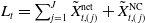 $L_t = \sum_{j= 1}^J \tilde{X}_{t,(\,j)}^{\text{net}} + \tilde{X}_{t, (\,j)}^{\text{NC}}$
represents the total claims liabilities at time t. This ratio measures the severity of the market deficit conditional on insolvency and is analogous to the Loss-Given-Default (LGD) metric used in reinsurance credit risk (Chen et al. Reference Chen, Cummins, Sun and Weiss2020). Together, these risk measures provide a comprehensive assessment of both the likelihood and severity of adverse outcomes in the surplus process.
$L_t = \sum_{j= 1}^J \tilde{X}_{t,(\,j)}^{\text{net}} + \tilde{X}_{t, (\,j)}^{\text{NC}}$
represents the total claims liabilities at time t. This ratio measures the severity of the market deficit conditional on insolvency and is analogous to the Loss-Given-Default (LGD) metric used in reinsurance credit risk (Chen et al. Reference Chen, Cummins, Sun and Weiss2020). Together, these risk measures provide a comprehensive assessment of both the likelihood and severity of adverse outcomes in the surplus process.
2.6. Benchmark model: Stationary DFA
For benchmarking purposes, we consider a stationary DFA model based on the main structure of the conventional DFA framework (see, e.g., Kaufmann et al. Reference Kaufmann, Gadmer and Klett2001). This model can be viewed as a special case of the climate-dependent DFA obtained by suppressing all climate-related components. It is calibrated using the same data sources as the climate-dependent DFA, and its simulation results are compared with those from the climate-dependent DFA in Section 3.5.
2.6.1. Hazards model
Under the stationary specification, event frequency and severity follow time-invariant distributions (Kaufmann et al. Reference Kaufmann, Gadmer and Klett2001):
 \begin{equation} M_t^{(i)} \sim F(\kappa_1, \ldots, \kappa_p), \quad X_t^{(i), m} \sim G(\vartheta_1, \ldots, \vartheta_q),\end{equation}
where the parameters
 $\kappa_1, \ldots, \kappa_p$
and
$\kappa_1, \ldots, \kappa_p$
and
 $\vartheta_1, \ldots, \vartheta_q$
are constant over time. This corresponds to the climate-dependent hazard model in Section 2.2.2 with all coefficients on climate variables set to zero.
$\vartheta_1, \ldots, \vartheta_q$
are constant over time. This corresponds to the climate-dependent hazard model in Section 2.2.2 with all coefficients on climate variables set to zero.
2.6.2. Inflation rate
Inflation is modelled as a mean-reverting AR(1) process consistent with the baseline specification in (2.6). This is a special case of the climate-dependent inflation model obtained by setting the climate overlay component (i.e.,
 $i_{m}^{\text{Clim-Impact}}$
) in (2.7) to zero.
$i_{m}^{\text{Clim-Impact}}$
) in (2.7) to zero.
2.6.3. Interest rates
Interest rates are modelled using a mean-reverting AR(1) process, which can be viewed as a special case of the generalised one-factor CIR model in Kaufmann et al. (Reference Kaufmann, Gadmer and Klett2001) with
 $g = 0$
:
$g = 0$
:
 \begin{equation} r_t = m_r + \varphi_r (r_{t-1} - m_r) + (r_{t-1})^g \epsilon_r(t), \quad \epsilon_r(t) \sim N(0, \sigma_r^2).\end{equation}
This corresponds to the climate-dependent specification in Section 2.3.2 when the coefficient on scenario-dependent economic growth is set to zero.
2.6.4. Equity model
Excess equity returns are modelled as a stationary Normal distribution:
 \begin{equation} x_t \sim N\big(\mu_{{x}}, \sigma_{{x}}^2\big).\end{equation}
This is a special case of the climate-dependent equity model in Section 2.3.3, obtained by muting sensitivity to scenario-dependent production growth and energy variables. Implicitly, this assumes that future economic conditions follow historical patterns.
2.6.5. Liabilities, premiums, and surplus
Adopting a similar approach to Kaufmann et al. (Reference Kaufmann, Gadmer and Klett2001), the exposure growth under the stationary setting is modelled as:
 \begin{equation} \delta_t = \mu_{\omega} + \phi_{\omega} (\delta_{t-1} - \mu_{\omega}) + \epsilon_t^{\omega},\end{equation}
where
 $\delta_t = \Delta \omega_t / \omega_{t-1}$
denotes the growth rate of exposure units, with its long-run mean denoted as
$\delta_t = \Delta \omega_t / \omega_{t-1}$
denotes the growth rate of exposure units, with its long-run mean denoted as
 $\mu_{\omega}$
.
$\mu_{\omega}$
.
Gross premiums and surplus are computed in the same manner as in the climate-dependent DFA, except that hazard distributions are assumed stationary and independent of climate variables. While the calculation of base reinsurance premiums is similar in both frameworks, the climate-dependent DFA incorporates the impact of climate change on reinsurance capital when deriving the solvency uplift applied to reinsurance premiums, whereas the stationary DFA does not. As a result, the difference in final reinsurance premiums between the two frameworks reflects not only changes in the underlying base premiums due to evolving climate risk, but also the additional solvency uplift arising from climate-related impacts on reinsurance capital.
3. Application to the Australian general insurance market
After introducing the modelling framework for the climate-dependent DFA, this section presents numerical examples to demonstrate its application within the Australian general insurance market. Section 3.1 discusses the selection of weather covariates and distributional assumptions for modelling hazard losses, tailored to the region under study. Section 3.2 outlines the data sources and parameter calibrations used in the proposed framework; detailed descriptions of the data sources and calibration results are provided in the Online Appendix A. Section 3.3 analyses key simulation results from individual modules and discusses their potential financial implications for general insurers. Section 3.4 analyses and compares general insurers’ financial performance under different climate scenarios using both risk and return measures. The simulation results from the benchmark stationary DFA model are incorporated into the figures presented in Sections 3.3 and 3.4 to avoid duplication. A detailed comparison between the stationary and climate-dependent DFA simulation results is provided separately in Section 3.5.
3.1. Selection of weather covariates and distribution assumptions
While Section 2.2.2 presents a general framework for modelling hazard losses under the impact of climate change, the specific choice of distributions and candidate weather covariates for each hazard type must be tailored to the region under study.
Following the framework outlined in Section 2.2.2, we assume that the frequency and severity of catastrophe events follow:
 \begin{equation} M_t^{(i)} \sim \text{Poi}\big(\lambda\big(\boldsymbol{\Theta}_t^{(i)}\big)\big); \;\; X_t^{(i), m} \sim \text{LN}\big(\mu\big(\boldsymbol{\Theta}_t^{(i)}\big), \sigma^2\big),\end{equation}
where
 $\boldsymbol{\Theta}^{(i)}_t$
is a set of weather covariates for hazard type i. The Poisson distribution aligns with common practice in modelling the frequency of hazard events (see, e.g., Jagger et al. Reference Jagger, Elsner and Saunders2008, Reference Jagger, Elsner and Burch2011). Similarly, Log-Normal distribution is frequently used for modelling catastrophe losses due to its heavy-tailed nature (Kaufmann et al. Reference Kaufmann, Gadmer and Klett2001; McNeil et al. Reference McNeil, Frey and Embrechts2015), and it is also selected from a class of heavy-tailed candidates based on our data. The detailed discussion of the selected distributions based on the Australian data is provided in Online Appendix C.3.1. However, alternative distributions may provide a better fit for other datasets; hence, it is recommended to validate the distributional assumptions proposed here when applying the model to new data.
$\boldsymbol{\Theta}^{(i)}_t$
is a set of weather covariates for hazard type i. The Poisson distribution aligns with common practice in modelling the frequency of hazard events (see, e.g., Jagger et al. Reference Jagger, Elsner and Saunders2008, Reference Jagger, Elsner and Burch2011). Similarly, Log-Normal distribution is frequently used for modelling catastrophe losses due to its heavy-tailed nature (Kaufmann et al. Reference Kaufmann, Gadmer and Klett2001; McNeil et al. Reference McNeil, Frey and Embrechts2015), and it is also selected from a class of heavy-tailed candidates based on our data. The detailed discussion of the selected distributions based on the Australian data is provided in Online Appendix C.3.1. However, alternative distributions may provide a better fit for other datasets; hence, it is recommended to validate the distributional assumptions proposed here when applying the model to new data.
The distribution parameters are then modelled as:
 \begin{equation} \log\big(\lambda^{(i)}_t\big) = \boldsymbol{\beta}_{(i)}^{\prime}\boldsymbol{\Theta}_t^{(i)}; \;\; \mu^{(i)}_t = \boldsymbol{\alpha}_{(i)}^{\prime}\boldsymbol{\Theta}_t^{(i)},\end{equation}
where the set of coefficients
 $\boldsymbol{\beta}_{(i)}$
and
$\boldsymbol{\beta}_{(i)}$
and
 $\boldsymbol{\alpha}_{(i)}$
are estimated via regression. We do not explicitly adjust the scale parameter of the severity distribution in this study. However, it could be modelled as a function of climate covariates using GAMLSS regression (Stasinopoulos and Rigby Reference Stasinopoulos and Rigby2008). This is left for future research when stronger statistical and climate science evidence becomes available on the influence of climate covariates on the scale parameter.
$\boldsymbol{\alpha}_{(i)}$
are estimated via regression. We do not explicitly adjust the scale parameter of the severity distribution in this study. However, it could be modelled as a function of climate covariates using GAMLSS regression (Stasinopoulos and Rigby Reference Stasinopoulos and Rigby2008). This is left for future research when stronger statistical and climate science evidence becomes available on the influence of climate covariates on the scale parameter.
Here, we focus on major Australian hazards: flood, bushfire, tropical cyclones, storms, hailstorm, and East Coast Lows (ECLs) (Insurance Council of Australia 2024). Below, we outline the candidate weather covariates for each hazard type, drawn from relevant literature on the associated physical processes. Although the data primarily cover Australia, the selection of candidate climate variables can be generalised to other regions, except for ECLs, which is a unique hazard type occurring near the eastern coast of Australia.
Bushfire. Bushfire risk depends on temperature, relative humidity, drought conditions, and wind speed (Sharples et al. Reference Sharples, Cary, Fox-Hughes, Mooney, Evans, Fletcher, Fromm, Grierson, McRae and Baker2016; Dowdy Reference Dowdy2018; Quilcaille et al. Reference Quilcaille, Batibeniz, Ribeiro, Padrón and Seneviratne2022). Generally, fire danger increases with higher temperatures, lower humidity, stronger winds, and more severe drought. The Fire Weather Index (FWI), derived from these factors, is commonly used to assess bushfire risk (Dowdy Reference Dowdy2018; Quilcaille et al. Reference Quilcaille, Batibeniz, Ribeiro, Padrón and Seneviratne2022). In particular, bushfire occurrence responds most strongly to extremes of the FWI rather than average conditions (Quilcaille et al. Reference Quilcaille, Batibeniz, Ribeiro, Padrón and Seneviratne2022). Hence, we choose
 \begin{align*}\boldsymbol{\Theta}_t^{\text{(BF)}} = \{\text{fwixx}_t, \text{fwixd}_t\},\end{align*}
where
 $\text{fwixx}_t$
is the annual maxima of fire weather index and
$\text{fwixx}_t$
is the annual maxima of fire weather index and
 $\text{fwixd}_t$
is the number of days with extreme fire weather, which are two crucial statistics capturing FWI extremes (Quilcaille et al. Reference Quilcaille, Batibeniz, Ribeiro, Padrón and Seneviratne2022). The FWI data is subsequently averaged over the land surface area of the selected country to derive a national-level indicator.
$\text{fwixd}_t$
is the number of days with extreme fire weather, which are two crucial statistics capturing FWI extremes (Quilcaille et al. Reference Quilcaille, Batibeniz, Ribeiro, Padrón and Seneviratne2022). The FWI data is subsequently averaged over the land surface area of the selected country to derive a national-level indicator.
Flood. Precipitation, particularly extreme precipitation, is a key driver of pluvial and river floods (Kodra et al. Reference Kodra, Bhatia, Chatterjee, Chen and Ganguly2020). Accordingly, we choose
 \begin{align*}\boldsymbol{\Theta}_t^{\text{(FL)}} = \big\{R^{\text{x5}}_t, R^{\text{x1}}_t, R_t\big\},\end{align*}
where
 $R_t$
represents the annual total precipitation,
$R_t$
represents the annual total precipitation,
 $R^{\text{x1}}_t$
is the largest one-day precipitation (usually denoted as rx1day), and
$R^{\text{x1}}_t$
is the largest one-day precipitation (usually denoted as rx1day), and
 $R^{\text{x5}}_t$
is the largest five-day cumulative precipitation (usually denoted as rx5day). Both
$R^{\text{x5}}_t$
is the largest five-day cumulative precipitation (usually denoted as rx5day). Both
 $R^{\text{x1}}_t$
and
$R^{\text{x1}}_t$
and
 $R^{\text{x5}}_t$
are commonly used as proxies for extreme precipitation in the IPCC report (Chapter 11 of IPCC 2021a
, pp. 1557–1561). Similarly, the precipitation data is then averaged across the land surface area of the selected country.
$R^{\text{x5}}_t$
are commonly used as proxies for extreme precipitation in the IPCC report (Chapter 11 of IPCC 2021a
, pp. 1557–1561). Similarly, the precipitation data is then averaged across the land surface area of the selected country.
Tropical cyclone and storms. The critical climate drivers for the formation and intensity of cyclones include sea surface temperature (SST) and sea level pressure (Meiler et al. Reference Meiler, Vogt, Bloemendaal, Ciullo, Lee, Camargo, Emanuel and Bresch2022). Warm ocean water is an essential condition for storm formation; additionally, low sea level pressure contributes to storm development by causing warm, moist air to rise (Bureau of Meteorology 2023). Therefore, storms typically form under conditions of high SST and low sea level pressure. When the wind speed exceeds 119 km/h, the storm is classified as a cyclone (Bureau of Meteorology 2023).
To capture the influence of SST and sea level pressure on tropical cyclones and storms, we choose
 \begin{align*}\boldsymbol{\Theta}_m^{\text{(TC)}} = \{\overline{\text{SST}}_m, \overline{\text{MSLP}}_m \},\end{align*}
where
 $\overline{\text{SST}}_m$
denotes the monthly average SST over the tropical cyclone basin near the selected country (e.g., the Australian Tropical Cyclone Basin for Australian applications),Footnote
4
and
$\overline{\text{SST}}_m$
denotes the monthly average SST over the tropical cyclone basin near the selected country (e.g., the Australian Tropical Cyclone Basin for Australian applications),Footnote
4
and
 $\overline{\text{MSLP}}_m$
is the monthly average mean sea level pressure over the same region. The use of monthly averages for SST and mean sea level pressure is also consistent with common practices in the literature, such as in the CAT model STORM (Bloemendaal et al. Reference Bloemendaal, Haigh, de Moel, Muis, Haarsma and Aerts2020).
$\overline{\text{MSLP}}_m$
is the monthly average mean sea level pressure over the same region. The use of monthly averages for SST and mean sea level pressure is also consistent with common practices in the literature, such as in the CAT model STORM (Bloemendaal et al. Reference Bloemendaal, Haigh, de Moel, Muis, Haarsma and Aerts2020).
Hailstorm. Atmospheric and near-surface temperatures are key drivers of hailstorm formation and intensity (Raupach et al. Reference Raupach, Martius, Allen, Kunz, Lasher-Trapp, Mohr, Rasmussen, Trapp and Zhang2021). Rising near-surface temperatures increase low-level moisture and convective instability, potentially boosting hail frequency (Allen et al. Reference Allen, Karoly and Walsh2014; Raupach et al. Reference Raupach, Martius, Allen, Kunz, Lasher-Trapp, Mohr, Rasmussen, Trapp and Zhang2021). Higher atmospheric temperatures contribute to greater water vapour, intensifying hailstorms, but also raise the melting level, which can reduce hail frequency by melting smaller hailstones (Raupach et al. Reference Raupach, Martius, Allen, Kunz, Lasher-Trapp, Mohr, Rasmussen, Trapp and Zhang2021). Thus, the overall impact varies locally. For instance, an increase in hail frequency is projected in Australia (Leslie et al. Reference Leslie, Leplastrier and Buckley2008; Allen et al. Reference Allen, Karoly and Walsh2014; Raupach et al. Reference Raupach, Martius, Allen, Kunz, Lasher-Trapp, Mohr, Rasmussen, Trapp and Zhang2021).
Accordingly, we choose
 \begin{align*}\boldsymbol{\Theta}_m^{\text{(H)}} = \big\{ \bar{T}_m^{\text{NS}}, \bar{T}_m^{\text{MT}} \big\},\end{align*}
where
 $\bar{T}_m^{\text{NS}}$
is the monthly average near-surface temperature and
$\bar{T}_m^{\text{NS}}$
is the monthly average near-surface temperature and
 $\bar{T}_m^{\text{MT}}$
is the monthly average mid-tropospheric temperature.
$\bar{T}_m^{\text{MT}}$
is the monthly average mid-tropospheric temperature.
East Coast Lows. An ECL is a type of mid-latitude cyclone that forms near the east coast of Australia, commonly referred to as the ECL identification region (Pepler et al. Reference Pepler, Alexander, Evans and Sherwood2016a ,Reference Pepler, Di Luca, Ji, Alexander, Evans and Sherwood b ; Speer et al. Reference Speer, Leslie, Hartigan and MacNamara2021). However, the formation mechanisms of ECLs differ from those of tropical cyclones. While tropical cyclones develop over warm ocean waters, ECL formation is primarily driven by SST gradients (Pepler et al. Reference Pepler, Alexander, Evans and Sherwood2016a ). The ECL module presented here is specifically designed for Australian applications; for use in other countries, this module may require modification or removal.
Based on the above mechanism, we choose
 \begin{align*}\boldsymbol{\Theta}_m^{\text{(ECL)}} = \{ \Delta \overline{\text{SST}}_m, \overline{\text{SST}}_m \},\end{align*}
where
 $\Delta \overline{\mathrm{SST}}_m$
represents the SST gradient near the east coast of Australia, defined as the average SST anomaly in the region
$\Delta \overline{\mathrm{SST}}_m$
represents the SST gradient near the east coast of Australia, defined as the average SST anomaly in the region
 $24^\circ$
–
$24^\circ$
–
 $41^\circ\mathrm{S}$
and
$41^\circ\mathrm{S}$
and
 $148^\circ$
–
$148^\circ$
–
 $155^\circ\mathrm{E}$
relative to the SST at the same latitudes and time between
$155^\circ\mathrm{E}$
relative to the SST at the same latitudes and time between
 $160^\circ$
–
$160^\circ$
–
 $165^\circ\mathrm{E}$
(Pepler et al. Reference Pepler, Alexander, Evans and Sherwood2016a
).
$165^\circ\mathrm{E}$
(Pepler et al. Reference Pepler, Alexander, Evans and Sherwood2016a
).
3.2. Data and calibration
The climate and hazard modules are calibrated using historical weather data from ERA 5 reanalysis (Copernicus Climate Change Service 2024b ) and future projections from CMIP 6 models (Copernicus Climate Change Service 2024a ) under various emissions scenarios.
Catastrophe frequency and severity are calibrated using the Insurance Council of Australia (ICA) dataset (Insurance Council of Australia 2024), with insured losses normalised for the Consumer Price Index (CPI) and exposure. Hazard models are selected based on both physical relevance (see Section 3.1) and statistical performance.
Macroeconomic models are calibrated using the Reserve Bank of Australia (RBA) cash rate data (Reserve Bank of Australia 2024), World Bank estimates of potential GDP growth (Kilic Celik et al. Reference Kilic Celik, Kose, Ohnsorge and Ruch2023), and CPI data from the Australian Bureau of Statistics (ABS) (Australian Bureau of Statistics 2024a ). The equity models are calibrated using corporate operating profits data from the ABS (Australian Bureau of Statistics 2024a ) and All Ordinaries total return data (FactSet 2024).
Insurance market assumptions and non-catastrophe loss calibrations are informed by the APRA’s General Insurance Performance and Institution-Level Statistics databases (APRA 2024a , b ).
Detailed data descriptions, calibration procedures, and results are provided in Online Appendix A. The calibration results for the stationary DFA model described in Section 2.6 are provided in Online Appendix B, using the same data sources listed above.
3.3. Key simulation results from individual modules
3.3.1. Climate and hazards
The simulated climate variables derived from the CMIP6 model outputs (Copernicus Climate Change Service 2024a ) are presented in Appendix A. Most variables show an upward trend, especially under high-emission scenarios, indicating a general increase in climate risk. The projections also exhibit notable inter-annual variability and a high degree of uncertainty, both of which are important drivers for the results shown in the downstream modules.
Simulation results of normalised hazard losses. Solid lines (and dotted lines under the stationary assumption) represent the average simulation paths under different climate scenarios, while dashed lines denote the
 $5^{\text{th}}$
and
$5^{\text{th}}$
and
 $95^{\text{th}}$
percentiles. Results are derived from simulated climate variables and calibrated hazard models. The simulations reveal an increasing trend in both the mean and volatility of hazard losses for most hazard types under high-emission scenarios.
$95^{\text{th}}$
percentiles. Results are derived from simulated climate variables and calibrated hazard models. The simulations reveal an increasing trend in both the mean and volatility of hazard losses for most hazard types under high-emission scenarios.

Based on the simulated climate variables, catastrophe losses for each hazard type are generated using the calibrated relationships between climate variables and hazard frequency and severity (see Figure 5). Overall, the projected normalised losses exhibit an increasing trend for most hazards, particularly under high-emission scenarios, with notable increases in both the mean and the upper tails of the loss distributions. In addition, the projected losses exhibit substantial inter-annual variability. For example, a pronounced peak in simulated flood losses is observed around 2047, particularly at the
 $95^{\text{th}}$
percentile. This peak is primarily driven by the corresponding increase in extreme precipitation (see Online Appendix D.1), which may be explained by the projected rise in the frequency of extreme ENSO events under high-emission scenarios reported in the literature (see, e.g., Cai et al. Reference Cai, Wang, Santoso, McPhaden, Wu, Jin, Timmermann, Collins, Vecchi, Lengaigne, England, Dommenget, Takahashi and Guilyardi2015; Heede and Fedorov Reference Heede and Fedorov2023). Moreover, the results reveal considerable uncertainty, driven by both the variability in simulation of climate variables as shown in Appendix A and the heavy-tailed nature of catastrophe losses. The rising mean and volatility are expected to place upward pressure on both insurance and reinsurance premiums, as well as shocks to capital over time.
$95^{\text{th}}$
percentile. This peak is primarily driven by the corresponding increase in extreme precipitation (see Online Appendix D.1), which may be explained by the projected rise in the frequency of extreme ENSO events under high-emission scenarios reported in the literature (see, e.g., Cai et al. Reference Cai, Wang, Santoso, McPhaden, Wu, Jin, Timmermann, Collins, Vecchi, Lengaigne, England, Dommenget, Takahashi and Guilyardi2015; Heede and Fedorov Reference Heede and Fedorov2023). Moreover, the results reveal considerable uncertainty, driven by both the variability in simulation of climate variables as shown in Appendix A and the heavy-tailed nature of catastrophe losses. The rising mean and volatility are expected to place upward pressure on both insurance and reinsurance premiums, as well as shocks to capital over time.
Remark 3.1. Despite the simplified structure of our hazard models, the simulation results generally align with physical risk trends reported in the literature. Projected increases in bushfire (with the upward trend more clearly illustrated in the extended simulation results presented in Online Appendix D.2) and flood losses are consistent with previous findings (Chapter 12 of IPCC 2021b , pp. 1805–1811), reflecting intensified extreme fire weather and increased extreme precipitation across much of Australia.
For tropical cyclones, existing literature suggests a decline in total cyclone numbers but a rise in high-intensity events (Chapter 12 of IPCC 2021b, pp. 1809–1810). As our frequency models are based on the ICA dataset, which only includes catastrophe-level hazards, the projected increase reflects trends in severe tropical cyclones and is broadly consistent with the literature.
Regarding hailstorms, a net increase in losses is projected. This is primarily driven by the influence of near-surface temperatures on storm frequency (see Table A in Online Appendix A.2) and aligns with expected increases in hailstorm frequency (Leslie et al. Reference Leslie, Leplastrier and Buckley2008; Allen et al. Reference Allen, Karoly and Walsh2014; Raupach et al. Reference Raupach, Martius, Allen, Kunz, Lasher-Trapp, Mohr, Rasmussen, Trapp and Zhang2021).
For ECLs, simulations show a slight decreasing trend, driven by changes in SST gradients. This result is consistent with studies projecting reduced ECL frequency under high-emission scenarios (Pepler et al. Reference Pepler, Alexander, Evans and Sherwood2016a ,Reference Pepler, Di Luca, Ji, Alexander, Evans and Sherwood b ; Speer et al. Reference Speer, Leslie, Hartigan and MacNamara2021).
Our focus is on broad trends in hazard losses rather than precise magnitudes, as the analysis aims to capture industry-wide patterns. For granular decision-making – such as capital allocation or portfolio steering – insurers can use proprietary claims data to tailor hazard models to their specific exposures.
3.3.2. Investment returns
The simulation results for the cumulative returns on the total investment portfolios, presented on a logarithmic scale, are shown in Figure 6(a).Footnote 5 The uncertainty bounds in the figure account for historical fluctuations in interest rates and equity returns, as well as the variability in climate-related damage to production available for consumption, as illustrated in Figure 7(a) and derived via (2.12).
Simulated (log) compounded investment returns (a) and projected compounded real GDP growth in Australia (b). Panel (a) shows the simulated compounded returns on the total investment portfolios generated from the economic growth assumptions and the simulated hazard losses underlying each scenario. Panel (b) presents compounded real GDP growth projections derived from the SSP database (Riahi et al. Reference Riahi, Van Vuuren, Kriegler, Edmonds, O’Neill, Fujimori, Bauer, Calvin, Dellink, Fricko, Lutz, Popp, Crespo Cuaresma, Samir, Leimbach, Jiang, Kram, Rao, Emmerling, Ebi and Tavoni2017).

Ratios of uninsured (a) and total (b) catastrophe losses to GDP. The results are obtained by dividing the scaled outputs from the hazard module (see Section 2.3.3) by the corresponding GDP projections under each climate scenario.

The observed trends in cumulative investment returns are primarily driven by the economic growth assumptions underlying each SSP scenario (Figure 6(b)). Under SSP 8.5, the highest cumulative investment return is projected, driven by its robust economic growth assumption (O’Neill et al. Reference O’Neill, Kriegler, Ebi, Kemp-Benedict, Riahi, Rothman, Van Ruijven, Van Vuuren, Birkmann, Kok, Levy and Solecki2017), followed by SSP 2.6. Conversely, SSP 7.0 exhibits the weakest cumulative investment return, influenced by both its slow economic growth assumptions and high catastrophe damages, in line with its narrative (O’Neill et al. Reference O’Neill, Kriegler, Ebi, Kemp-Benedict, Riahi, Rothman, Van Ruijven, Van Vuuren, Birkmann, Kok, Levy and Solecki2017). The relatively high investment returns under SSP 8.5 and SSP 2.6 are likely to accelerate capital accumulation. By contrast, the lower returns, coupled with high catastrophe losses in SSP 7.0 (see Figures 7(b) and 5), are expected to slow the pace of capital accumulation under this scenario. A sensitivity analysis using alternative economic damage assumptions has also been conducted (see Online Appendix I), indicating broadly consistent patterns with those reported in this section.
A breakdown analysis of investment returns for the general and brown portfolios is provided in Online Appendix E.2. Overall, the transition stress remains relatively mild, as the SSP scenarios considered do not assume abrupt or disorderly transitions, as noted in Limitation 2.1.
3.3.3. Premiums and underwriting losses
The normalised gross premiums associated with catastrophe (CAT) coverage are presented in Figure 8(a). An overall increasing trend is found, driven by the rising risk of most hazards as shown in Figure 5. Gross CAT premiums reach their highest levels under SSP 8.5, particularly in the later projection period, followed by SSP 7.0, SSP 4.5, and SSP 2.6, in line with the physical risk narratives underlying those scenarios as described in Section 2.1. The increase in premiums may also create affordability issues and, as noted in Limitation 2.7, affect insurance demand. This effect is noted as a limitation of the current paper but is encouraged for future research. In addition to this general upward trend, significant inter-annual variability is observed, reflecting the internal climate variability of the underlying climate variables as shown in Appendix A.
Gross premiums (normalised) associated with catastrophe cover, shown as dollar values (a) and as a proportion of total gross premiums (b). Panel (a) presents the normalised values of calculated gross catastrophe (CAT) premiums based on (2.19). Panel (b) shows the projected CAT premiums as a proportion of total premiums, compared with historically observed CAT losses as a share of total insurance losses, based on data from the APRA database and the ICA dataset. Both panels indicate an increasing trend in CAT premiums – both in dollar terms and as a share of total premiums – particularly under high-emission scenarios.

Moreover, the proportion of CAT premiums relative to total general insurance premiums is expected to increase relative to the historical levels, with a more pronounced increase under high-emission scenarios. This is illustrated in Figure 8(b), which compares projected CAT premium proportions with historically observed CAT loss proportions (used here as a proxy for historical CAT premium proportions) derived from the General Insurance Performance Database (APRA 2024b ) and the ICA dataset. These findings suggest that catastrophe losses will have an increasingly significant impact on the underwriting performance of general insurers under the influence of climate change. Consequently, managing CAT exposures will become a more critical component of portfolio management for general insurers.
A similar pattern to the gross insurance premiums emerges in the reinsurance premiums (Figure 9(a)), which show a general upward trend. The highest projected premium occurs under SSP 8.5, followed by SSP 7.0, while SSP 2.6 is expected to have the lowest premium.
Total reinsurance premiums (normalised) (a) and relative difference between total and base reinsurance premiums (b). Panel (a) shows the normalised values of calculated total reinsurance premiums (including mark-up), averaged across simulation paths, based on (2.21). The results exhibit trends similar to those observed for gross CAT premiums. Panel (b) presents the relative difference between total reinsurance premiums and base reinsurance premiums, with the latter calculated using (2.20). The largest premium uplift is projected under the SSP 7.0 scenario.

To illustrate the role of reinsurance capital constraints, Figure 9(b) presents the average relative difference between the solvency-sensitive reinsurance premiums (in (2.20)) and the base premiums (in (2.21)). The largest uplift appears under SSP 7.0, likely due to low investment returns coupled with high insurance losses (Sections 3.3.1 and 3.3.2), resulting in slower capital accumulation and prolonged tight capacity. In contrast, SSP 8.5 exhibits the smallest uplift despite experiencing the highest catastrophe (CAT) losses, possibly because its stronger investment returns (see Section 3.3.2) accelerate capital accumulation and shorten tight-capacity periods. A similar pattern is also observed in the primary general insurance market (see Section 3.4).
The results also suggest that the percentage growth in reinsurance premiums exceeds that of primary insurance, reflecting both rising physical risks and adjustments to tightening reinsurance capital. The modelled uplift relative to the base level is considered as conservative due to the simplified assumptions outlined in Limitation 2.8. Nevertheless, it is assumed that primary insurers will continue to purchase reinsurance despite higher prices; however, rising premiums may dampen demand, although this effect could be partly offset by the strengthening risk-transfer demand as climate risk intensifies (Lloyd’s 2025). The dynamics of these effects are left for future research.
Using the calculated premiums and simulated catastrophe losses from the hazard module (Section 3.3.1), we derive the simulated underwriting losses, with normalised results presented in Figure 10. On average, the simulated underwriting loss remains below zero (indicating a positive underwriting profit) and is relatively consistent across scenarios, which could be explained by the premium loadings. At higher quantiles, however, underwriting losses remain similar across scenarios initially but rise substantially in later periods under high-emission pathways (SSP 8.5 and SSP 7.0) due to escalating climate risks. This upward shift in the tail of underwriting losses can be attributed to the increasing volatility and extreme percentile of hazard losses observed under high-emission scenarios (see Section 3.3.1). Consequently, while downside liability impacts on financial performance appear moderate at first, they are expected to intensify over longer projection horizons in the high-emission scenarios.
Simulations of underwriting losses (normalised). Underwriting losses are calculated by subtracting the net premium received (i.e., gross premium received minus reinsurance premiums paid) from the net simulated insurance losses (i.e., gross insurance losses net of reinsurance recoverables). Solid lines (and dotted lines under the stationary assumption) represent the average simulation paths across climate scenarios, while dashed lines indicate the
 $5^{\text{th}}$
and
$5^{\text{th}}$
and
 $95^{\text{th}}$
percentiles. Across climate scenarios, the results are similar at the mean level but diverge at higher quantiles, with greater losses projected under high-emission scenarios.
$95^{\text{th}}$
percentiles. Across climate scenarios, the results are similar at the mean level but diverge at higher quantiles, with greater losses projected under high-emission scenarios.

3.4. Risk and returns measures
Finally, the risk and return measures for the general insurance market can be derived from the surplus, which is calculated using outputs from the individual modules (see (2.23)). Figure 11(a) and (b) show the expected and median surplus, which are our return measures, across different SSP scenarios. Under SSP 8.5, surplus is highest, followed by SSP 2.6, whereas SSP 7.0 yields the lowest surplus.
Expected (a) and median (b) market surplus (log scale) derived from surplus simulations. Both the expected and median surplus trajectories reflect the economic growth assumptions underlying each climate scenario.

To investigate the drivers of these surplus trends, we compare the expected and median surplus with cumulative investment returns at their average and median paths, revealing that differences in cumulative investment returns largely explain the observed surplus patterns (see Appendix B). These findings align with earlier results showing that underwriting profits or losses are similar at mean levels across scenarios (Section 3.3.3), making investment growth the primary driver of mean and median surplus trends. Since investment returns are predominantly affected by the economic growth assumptions underlying each scenario (Section 3.3.2), the divergent economic growth paths in different SSP scenarios are expected to be the key drivers of expected returns to the general insurance industry.
Figure 12(a) shows market insolvency probabilities under various scenarios, a common risk metric in DFA studies (Kaufmann et al. Reference Kaufmann, Gadmer and Klett2001). SSP 7.0 exhibits the highest insolvency rates, followed by SSP 4.5 and SSP 2.6. Although SSP 7.0 does not incur the highest hazard losses, its poor investment returns (Section 3.3.2), substantial reinsurance premium increases (Section 3.3.3), and relatively high catastrophe (CAT) losses (Section 3.3.1) collectively erode profits and constrain capital accumulation, leading to high insolvency probabilities once both physical and economic aspects of the climate change are considered. These outcomes align with the physical and economic narratives underlying the SSP 7.0 scenario (Section 2.1).
Market insolvency probabilities (a) and market deficit-given-insolvency ratiosFootnote
6
(b). Panel (a) shows the proportion of simulations in which total market capital becomes negative, while Panel (b) presents the ratio of market deficit to total claims liabilities, conditional on market insolvency. Solid lines (and dotted lines under the stationary assumption) represent the average simulation paths across climate scenarios, and dashed lines indicate the
 $5^{\text{th}}$
and
$5^{\text{th}}$
and
 $95^{\text{th}}$
percentiles. The SSP 8.5 scenario exhibits the lowest market insolvency probability but the highest market deficit-given-insolvency ratio.
$95^{\text{th}}$
percentiles. The SSP 8.5 scenario exhibits the lowest market insolvency probability but the highest market deficit-given-insolvency ratio.

Interestingly, while SSP 8.5 is typically linked to the highest physical risks in climate science (Chapter 11 of IPCC 2021a , pp. 1517–1605), it yields the lowest projected insolvency probabilities when both physical and economic factors are modelled. This outcome stems from strong investment returns outpacing underwriting losses early in the projection horizon (see Figures 6(a) and 10). As a result, capital accumulates rapidly, particularly in the early years. SSP 8.5 also shows the highest average Compound Annual Growth Rate (CAGR) of market surplusFootnote 7 (see Appendix C), which could help insurers absorb potential losses at later stages. These findings align with the SSP 8.5 narrative of “robust economic growth,” which leads to “low adaptation challenges” except in extreme case (O’Neill et al. Reference O’Neill, Kriegler, Ebi, Kemp-Benedict, Riahi, Rothman, Van Ruijven, Van Vuuren, Birkmann, Kok, Levy and Solecki2017).
However, when insolvency occurs, SSP 8.5 results in the most severe impacts in later projection horizons, as shown by the market deficit-given-insolvency ratios (see Figure 12(b)). These ratios, which indicate the share of unpaid claims, suggest that policyholders tend to face the greatest losses under SSP 8.5 in tail events. This is likely due to higher underwriting losses in the distribution tails later in the projection (Section 3.3.3; Figure 10), despite similar early-horizon losses across scenarios. Additionally, given the limitations of SSP 8.5 (Section 2.1), insurers should remain cautious about unmodelled risks such as economic collapse from climate tipping points.
SSP 2.6 offers a more balanced risk–return profile, with the second-highest expected surplus, second-lowest insolvency risk, and modest market deficits in insolvency. It also features the lowest projected catastrophe-related premiums, potentially enhancing affordability and insurance coverage against climate risks. These results align with SSP 2.6’s narrative of “sustainable economic development” and “improving environmental conditions,” leading to “low mitigation and adaptation challenges” (O’Neill et al. Reference O’Neill, Kriegler, Ebi, Kemp-Benedict, Riahi, Rothman, Van Ruijven, Van Vuuren, Birkmann, Kok, Levy and Solecki2017).
Remark 3.3. The results on surplus and insolvency probability presented in Section 3.4 are based on the assumption that no dividends are paid from the surplus, consistent with the paper’s objective of establishing a baseline model. We also conducted a sensitivity analysis to examine the impact of different dividend policies on surplus and insolvency probability. Overall, although the magnitudes of surplus and insolvency probability vary under different dividend policies, the scenario rankings with respect to surplus and insolvency probability under varying dividend payout assumptions remain consistent with the baseline findings reported in this section. It is also found that the SSP 8.5 scenario shows greater sensitivity to higher dividend payouts, as larger dividends erode the capital buffer to absorb high catastrophe losses under this scenario. Detailed results and discussions are provided in Online Appendix H.
3.5. Comparison with the stationary DFA model
We also compare the simulation results from the climate-dependent DFA model with those from the benchmark stationary DFA model specified in Section 2.6. The stationary DFA outcomes are shown as grey dotted lines in the figures presented in Sections 3.3 and 3.4. The main observations from this comparison are summarised below.
A key distinction between the two frameworks lies in the ability of the climate-dependent DFA to capture long-term climate trends embedded in the scenario assumptions. As illustrated by the simulations of hazard losses (Figure 5 in Section 3.3.1) and projected gross CAT premiums (Figure 8(a) in Section 3.3.3), the stationary DFA produces relatively stable mean hazard losses and premiums over time. In contrast, the climate-dependent DFA captures the upward trend in hazard losses and associated premiums under climate change, particularly under higher-emission scenarios. Moreover, the stationary DFA does not reflect inter-annual variability in hazard losses arising from internal climate dynamics (e.g., ENSO cycles). By linking climate model inputs to the hazard models, as described in Section 2.2.2, the climate-dependent DFA captures both long-term trends and short-term variability in hazard losses.
Another distinguishing feature of the climate-dependent DFA is its ability to incorporate different scenario assumptions. As shown in the simulated cumulative investment returns (Figure 6(a)) and the projected mean and median market surplus (Figure 11(b) and (a)), the stationary results are broadly similar to those under the SSP 2.6 and SSP 4.5 scenarios. However, the stationary DFA does not capture the trends observed under the higher-emission scenarios (SSP 7.0 and SSP 8.5). In particular, it tends to underestimate the insolvency probability if the SSP 7.0 scenario is realised (Figure 12(a)), as it does not incorporate the combination of weaker economic growth and elevated physical risks associated with this pathway. These factors lead to lower investment returns and higher underwriting losses, which jointly erode insurers’ capital over the long term. This highlights the advantage of the climate-dependent DFA in generating long-term projections under climate change, where future economic and physical conditions may differ substantially from the present environment.
A further difference lies in the ability of the climate-dependent DFA to capture uncertainty in future climate impacts. For example, in the simulated underwriting losses (Figure 10), the mean losses are broadly similar across scenarios, but the stationary DFA exhibits lower volatility and smaller upper-tail percentiles compared with the climate-dependent DFA. A similar pattern is observed in the individual hazard losses (Figure 5), where the stationary DFA produces consistently lower simulation volatility across hazard types. This difference reflects the additional model and stochastic uncertainty in future climate dynamics captured in the climate module of the climate-dependent DFA, which is subsequently propagated to the hazard and financial modules. Omitting this additional uncertainty may lead to an underestimation of tail risks when projecting future financial outcomes. Consistent with this observation, the market deficit given insolvency (Figure 12(b)) is notably lower under the stationary DFA than under the climate-dependent DFA, indicating a lower estimated severity of insolvency in the stationary case.
4. Discussion
The modelling framework necessarily adopts simplifying assumptions to manage the complexity of climate risk. While this offers a practical starting point, it introduces several key limitations that warrant attention. It also presents several opportunities for future extension, as discussed below.
4.1. Reliances and limitations
The first limitation of our analysis is its reliance on economic and environmental assumptions in the SSP scenarios, which have inherent limitations (see Limitation 2.1). In addition, post-disaster reconstruction effects have not been explicitly incorporated into adjusting the GDP assumptions for climate damage (see Limitation 2.6).
Second, our hazard loss forecasts rely on historically calibrated relationships between climate variables and insurance losses, which may shift over time. Future research could adopt a more forward-looking approach to reflect these changes (see Limitation 2.4).
Third, the framework is limited to domestic disasters and excludes global spillover effects. However, climate-related economic damage can potentially spread via international trade (Neal et al. Reference Neal, Newell and Pitman2025). Modelling these linkages would offer a more complete view of risks to local insurers.
Additionally, as noted in Limitation 2.7, the framework does not consider potential business volume loss from rising premiums. Also, the analysis does not incorporate possible changes in future building standards or dwelling sizes that may result from adaptation measures when projecting hazard losses.
Finally, while the framework incorporates several sources of climate-related uncertainty, it does not capture uncertainty arising from parameters and model inadequacy (see Limitation 2.5). The unidentified risks are also not quantified in our framework due to their unquantifiable and truly unknown nature (see Limitation 2.2). Users should therefore remain mindful of these additional risks and uncertainties when interpreting the model outputs.
4.2. Extensions and future work
Our framework offers several avenues for extension. First, as discussed in Remark 2.1, while this paper assesses climate risks at an industry-wide level, it provides a foundation for individual insurers to develop firm-specific, climate-dependent DFA models aligned with their unique risk profiles. In addition, the current modelling framework does not differentiate between lines of business. Although this simplification is appropriate for the study’s macro-level focus, future research could extend the framework to incorporate multiple business lines, which would be particularly useful for decision-making at the individual insurer level, such as capital allocation (Myers and Read Reference Myers and Read2001).
Second, as noted in Limitations 2.3 and 2.8, the model serves as a baseline that does not incorporate the effects of government interventions, market competition, or regulatory actions. While certain reinsurance market dynamics have been considered in this study, it should not be regarded as a comprehensive modelling of reinsurance cycles due to the simplified assumptions outlined in Limitation 2.8. Future research could incorporate these factors and compare the outcomes with this baseline to assess their impact on the financial performance of general insurers under different climate scenarios.
Third, on the liability side, the model focuses on climate impacts on catastrophe losses. Future research could extend this by incorporating climate effects on non-catastrophe losses as relevant data become available.
Moreover, as noted in Limitation 2.2, transition risks on the liability side are not yet included. Their integration could be explored in future work once quantification methods are more established in the literature.
Finally, the modelling approach is broad but simplified. Future studies may adopt more advanced component models for greater precision, such as the proprietary catastrophe (CAT) models. These enhancements, however, must be balanced against the trade-off between model complexity and parsimony, which is an essential consideration in DFA.
5. Conclusions
This paper extends the traditional DFA framework by incorporating climate change considerations. This extension represents a paradigm shift towards a forward-looking framework recognising that future economic and physical conditions may differ fundamentally from historical experience due to climate change. We show how climate-related impacts and scenario assumptions can systematically be integrated across the different modules of the DFA framework, drawing on insights from climate science, climate-economy literature, and the financial relationships embedded in conventional DFA models. This integrated structure allows the framework to capture the interdependencies between assets and liabilities under climate change, enabling a holistic assessment of climate-related impacts on general insurers that remains relatively under-explored in the literature. The proposed extension also translates climate scenario narratives into insurers’ balance-sheet outcomes in a tractable manner. By balancing tractability and comprehensiveness in the design of the component models, the framework captures the key assumptions of climate scenarios and the main characteristics of climate change impacts, while retaining the desirable features of conventional DFA frameworks, such as transparency and interpretability.
To illustrate the contributions of the proposed framework, we apply it to the Australian general insurance market. Compared with the results from a conventional stationary DFA model, the climate-dependent DFA captures not only the long-term trends associated with climate change and the differences across emission pathways but also the uncertainty surrounding future climate impacts. Ignoring these factors in financial projections may lead to a misestimation of insurers’ risk and return profiles under climate change and may consequently affect strategic decision-making.
The empirical illustration of the proposed framework also provides several useful insights into the potential impact of climate change on the general insurance market. In climate science, SSP 8.5 carries the highest physical risk, followed by SSP 7.0, SSP 4.5, and SSP 2.6 (Chapter 11 of IPCC 2021a , pp. 1517–1605), a ranking reflected in our hazard simulations and CAT premium projections. However, when both economic and physical factors are considered, SSP 7.0, which combines high catastrophe risk with poor economic growth, emerges as the most detrimental scenario for insurers, leading to low returns and high insolvency risk. In contrast, SSP 8.5 delivers the highest returns and lowest insolvency probability due to strong economic growth but also results in the largest market deficits upon insolvency, increasing risks to policyholders.
These findings highlight the need for insurers to prepare for scenarios involving both high catastrophe risk and weak economic growth in strategic areas such as business planning, capital management, and reinsurance. Insurers should also account for the tail-end financial risks under high-emission scenarios like SSP 8.5. Regulators, in turn, should ensure adequate capital buffers and collaborate with governments on contingency plans, such as bail-out mechanisms, to manage systemic risks from potential insurer insolvencies. Further development of the proposed climate-dependent DFA framework might support these efforts. Indeed, the framework developed in this paper provides a useful foundation for assessing climate-related financial risks, which can be further developed in many useful directions, as discussed in Section 4.2.
Supplementary material
The supplementary material for this article can be found at https://doi.org/10.1017/asb.2026.10102
Data and Code
The R code used in this study is available at https://github.com/agi-lab/climate-dependent-DFA, and the supporting datasets are hosted at https://zenodo.org/records/18521235. Instructions for data access and code execution are provided on the GitHub page.
Due to licensing restrictions, we cannot share the Total Returns series of the All-Ordinaries Shares Index; users should obtain it directly from FactSet. For those without access, pseudo data simulated from the calibrated equity model is provided for calibration.
Similarly, we cannot distribute Woodside Energy Limited’s 2014–2023 financial statements from FactSet. Users can retrieve them via FactSet or compile them manually from public reports at https://www.woodside.com/investors/reports-investor-briefings. For models using restricted datasets, the same parameters are applied in the code to ensure consistency with the results presented.
Acknowledgements
This research was supported under Australian Research Council’s Discovery Project (DP200101859) funding scheme and University International Postgraduate Award (UIPA). The views and opinions expressed in this paper are solely those of the authors and do not reflect those of their affiliated institutions.
The authors would like to extend their sincere gratitude to Sharanjit Paddam for his constructive feedback and insightful comments, which significantly improved the quality of this paper and provided valuable guidance for potential future research directions.
Earlier versions of this paper were presented at the 2024 Australasian Actuarial Education and Research Symposium (AAERS) in Melbourne (Australia), All Actuaries Summit 2025 in Sydney (Australia), the 2025 28th International Congress on Insurance: Mathematics and Economics held in Tartu (Estonia), the 2026 inaugural ASTIN Bulletin Conference, as well as at research seminars hosted by the School of Risk and Actuarial Studies at UNSW. The authors are grateful for constructive comments received from colleagues who attended those events.
The authors also gratefully acknowledge the Actuaries Institute of Australia for awarding the Melville Prize and the Carol Dolan Prize to an earlier version of this paper, which was tailored for an industry audience and presented at the All Actuaries Summit 2025.
Competing interests
None.
Appendix A. Simulation results of climate variables
Figure A1 presents the simulated climate variables derived from the CMIP6 model outputs (Copernicus Climate Change Service 2024a ). The results suggest that most climate variables, except for SST gradients, exhibit an upward trend, particularly under high-emission scenarios, indicating an overall increase in climate risk.
Simulation results for climate variables. Results are generated using CMIP6 model outputs and the simulation methodology described in Section 2.2.1. Solid lines represent the average simulation paths under different climate scenarios, while dashed lines indicate the
 $5^{\text{th}}$
and
$5^{\text{th}}$
and
 $95^{\text{th}}$
percentiles. The simulations illustrate both long-term trends and inter-annual variability, as well as the uncertainty associated with the projections.
$95^{\text{th}}$
percentiles. The simulations illustrate both long-term trends and inter-annual variability, as well as the uncertainty associated with the projections.

In addition to this long-term trend, the average simulation path also shows notable inter-annual variability. This variability, likely driven by internal climate processes (e.g., El Niño cycles) captured by the CMIP6 models (Jain et al. Reference Jain, Scaife, Shepherd, Deser, Dunstone, Schmidt, Trenberth and Turkington2023), may contribute to annual fluctuations in insurance premiums and costs as shown in the corresponding sections in the paper.
Furthermore, the projections display a high degree of uncertainty. This uncertainty, also highlighted in other studies (see, e.g., Wu et al. Reference Wu, Miao, Fan, Gou, Zhang and Zheng2022), arises from both the climate model uncertainty and the aleatoric uncertainty incorporated in our climate module (see Section 2.2.1). Given that such uncertainty, especially at the upper percentiles, is crucial for actuarial applications and capital modelling, these findings underscore the importance of accounting for uncertainty in climate projections, as discussed in Sections 1.2 and 2.2.1.
B. Relationships between market surplus and investment returns
Figure B1 illustrates the relationship between market surplus and investment returns at both the mean and median levels.
Expected (a) and median (b) market surplus versus average (a) and median (b) compounded investment returns (log scale). The results indicate a strong correlation between market surplus and compounded investment returns at both the mean and median levels.

C. Mean CAGR of market surplus
Figure C1 presents the mean Compound Annual Growth Rate (CAGR) of market surplus by projection horizon and climate scenario.
Mean Compound Annual Growth Rate (CAGR) of market surplus, by projection horizon and climate scenario. This metric reflects the rate of capital accumulation over different projection periods. The highest growth rate is observed under the SSP 8.5 scenario during the early projection horizon.


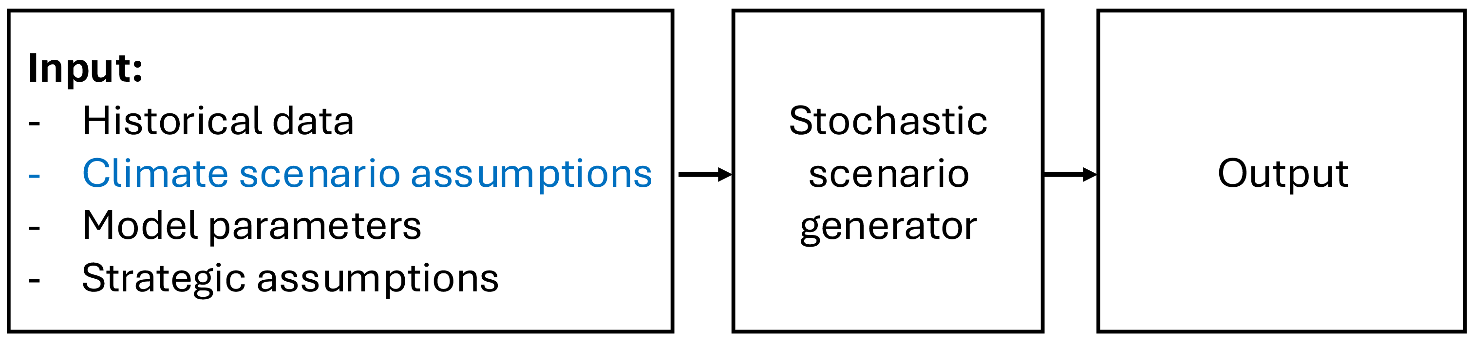


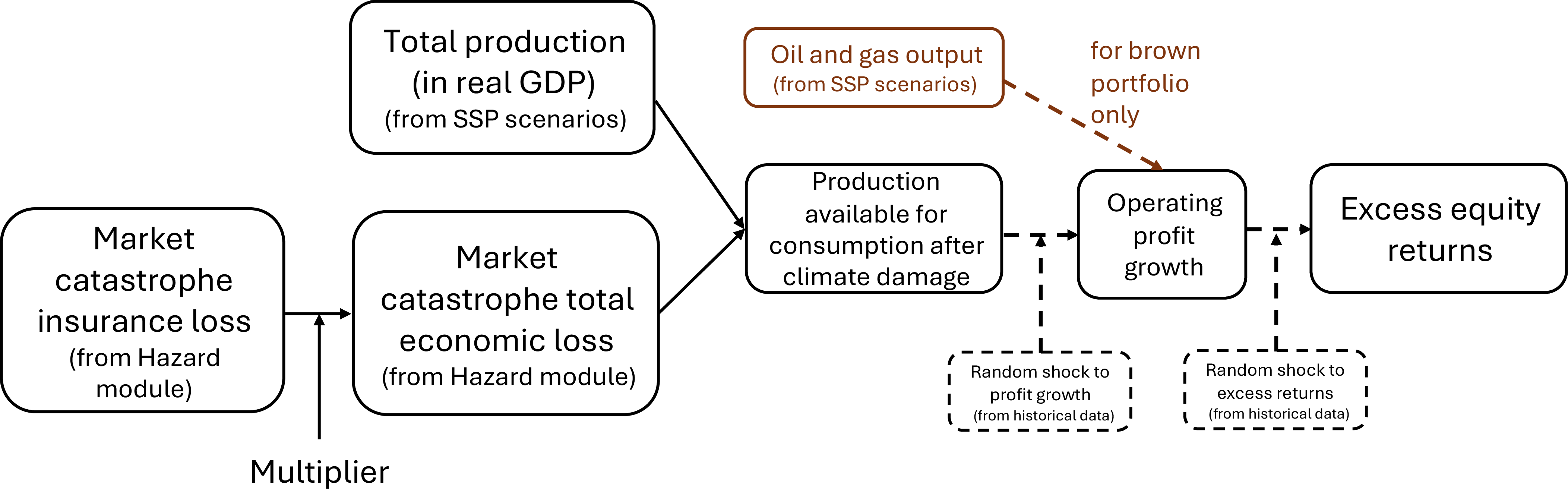


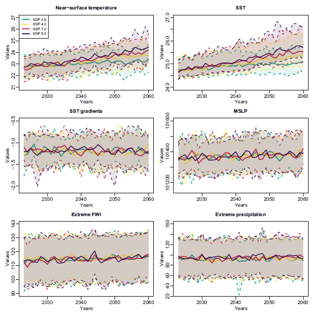


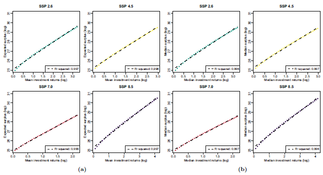
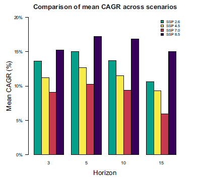


 Open access