


1. INTRODUCTION
Proglacial fjords act as conduits that transfer heat and mass between glaciers and the ocean. The rates of heat and mass transfer are affected by a number of processes, including subglacial discharge, wind and tides (Motyka and others, Reference Motyka, Hunter, Echelmeyer and Connor2003; Jackson and Straneo, Reference Jackson and Straneo2016; Spall and others, Reference Spall, Jackson and Straneo2017). Subglacial discharge is of particular interest because it mixes with warm saline water at depth and creates a vigorous upwelling plume that melts glacier termini. Submarine melting is an important component of tidewater glacier mass balance (Truffer and Motyka, Reference Truffer and Motyka2016), and subglacial discharge and submarine melt are key sources of freshwater for fjords (Moon and others, Reference Moon2017). In addition, upwelling plumes transport nutrients and entrain zooplankton (Arimitsu and others, Reference Arimitsu, Piatt and Mueter2016), thereby creating biological hotspots for sea birds and marine mammals (e.g., Lydersen and others, Reference Lydersen2014; Urbanski and others, Reference Urbanski2017). A detailed understanding of the processes driving fjord circulation is lacking, however, due to difficulties in observing these highly dynamic environments over long time scales at high spatial and temporal resolutions.
Fjord circulation is typically observed with Acoustic Doppler Current Profilers (ADCPs) that are either deployed on moorings or operated from vessels. ADCPs deployed on moorings provide high spatial resolution in the vertical domain, as well as good temporal coverage and resolution. In contrast, their horizontal coverage is limited to a single location. Also, moorings are difficult to deploy and retrieve in iceberg-filled waters, and may suffer damage from collisions with icebergs. ADCP measurements from moving vessels provide better spatial coverage than moorings, but lack temporal coverage and resolution at single locations. Spatial coverage may be limited by iceberg-rich water during field campaigns. In general, ADCPs are unable to capture velocities in the uppermost water layer due to side lobe interference or draft and ringing effects (e.g., Chen and others, Reference Chen, Wang, Liu, Wang and Leng2016). Here we present a complementary image-based tracking method to measure iceberg velocities and use them to infer near-surface currents. Based on oblique time-lapse photography, spatial patterns of currents can be determined over months to years, at temporal resolution on the order of minutes. Unlike ADCP measurements, this method is well suited for iceberg-filled waters and areas close to the calving front, with the caveat that it requires icebergs as tracers. Icebergs integrate currents across their submerged portion so that their velocities reflect average currents between the water surface and their (unknown) keel depth; wind drag above the water may further complicate the relationship between ice motion and water velocity (e.g., FitzMaurice and others, Reference FitzMaurice, Straneo, Cenedese and Andres2016). For best representation of near-surface currents, tracked icebergs should be small, which is typically the case in the LeConte Bay study area, but not necessarily in other fjords.
Image-based measurement of iceberg motion/fjord circulation is an emerging research field in glaciology and oceanography, exploiting satellite imagery (e.g., Enderlin and Hamilton, Reference Enderlin and Hamilton2014), ground-based radar imagery (Voytenko and others, Reference Voytenko2015; Olofsson and others, Reference Olofsson, Veibäck and Hendeby2017) and optical oblique photos (Schild and others, Reference Schild2018). By contrast, image-based measurement of glacier motion has been conducted for several decades, both on oblique photos (e.g., Krimmel and Rasmussen, Reference Krimmel and Rasmussen1986; Messerli and Grinsted, Reference Messerli and Grinsted2015; Schwalbe and Maas, Reference Schwalbe and Maas2017) and optical/radar satellite imagery (e.g., Scambos and others, Reference Scambos, Dutkiewicz, Wilson and Bindschadler1992; Rignot and others, Reference Rignot, Mouginot and Scheuchl2011; Rosenau and others, Reference Rosenau, Scheinert and Dietrich2015; Altena and Kääb, Reference Altena and Kääb2017). Compared with the relatively slow (order of m d−1), steady and predictable flow of glaciers, fjord surface currents are much faster (order of m s−1) and often rapidly changing. Observing fjord circulation with time-lapse photos therefore requires much higher frame rates than corresponding glacier studies, which are now possible thanks to advances in data storage capacity and computer processing.
Running up to five cameras between April 2016 and September 2017, we collected >400 000 images of LeConte Bay, Alaska, at rates of at least 0.5 min−1 (one image every 2 minutes). To process and analyze the images, we developed code based on the Python programming language and the computer vision library OpenCV (https://opencv.org). Specifically, we use OpenCV's implementation of the Lucas-Kanade tracker, a well-established optical flow algorithm. In this paper, we present the image-tracking method, address technical issues such as requisite temporal and spatial resolution of imagery, ground truth our velocity calculations with ADCP data and demonstrate the method's utility by quantifying subdaily to seasonal patterns in near-surface currents. Our results will put constraints on forthcoming analysis of oceanographic data and hydrodynamic modeling efforts.
2. STUDY SITE
LeConte Bay (56.80°N, 132.45°W) is a 25 km long fjord between Frederick Sound and LeConte Glacier in Southeast Alaska (Fig. 1a). Forty kilometer long LeConte Glacier ranges in elevation from sea level to 2800 m, draining 477 km2 ( $\scriptstyle \sim $8%) of the Stikine Icefield (Kienholz and others, Reference Kienholz2015). In the glacier's lowest reaches, the ice is funneled through a narrow valley and ultimately lost by calving and submarine melting, with submarine melting accounting for up to half of the frontal ablation seasonally (Motyka and others, Reference Motyka, Dryer, Amundson, Truffer and Fahnestock2013). Ice speeds reach $\scriptstyle \sim $25 m d−1 near LeConte's calving front (O'Neel and others, Reference O'Neel, Echelmeyer and Motyka2003). The proglacial fjord experiences a net estuarine circulation heavily influenced by freshwater runoff from the glacier, which can exceed 400 m3 s−1 during rain and melt events (Motyka and others, Reference Motyka, Hunter, Echelmeyer and Connor2003, Reference Motyka, Dryer, Amundson, Truffer and Fahnestock2013) and result in near-glacier surface currents in excess of 1 m s−1. Wind and semi-diurnal tides, with amplitudes exceeding 6 m during spring tides, modulate the circulation pattern.
(a) Landsat-8 image of LeConte Glacier, LeConte Bay, and the town of Petersburg. (b) WorldView-2 image (Ⓒ 2011, DigitalGlobe, Inc.) of LeConte Bay and LeConte Glacier overlain by the cameras' fields of view (colored lines). (c) Photo of cameras 1–3, which were co-located on granitic bedrock  $\scriptstyle \sim $420 m above LeConte Bay. (d, e) Photos taken from cameras 4 and 3 with locations of the mooring and surveying transects.
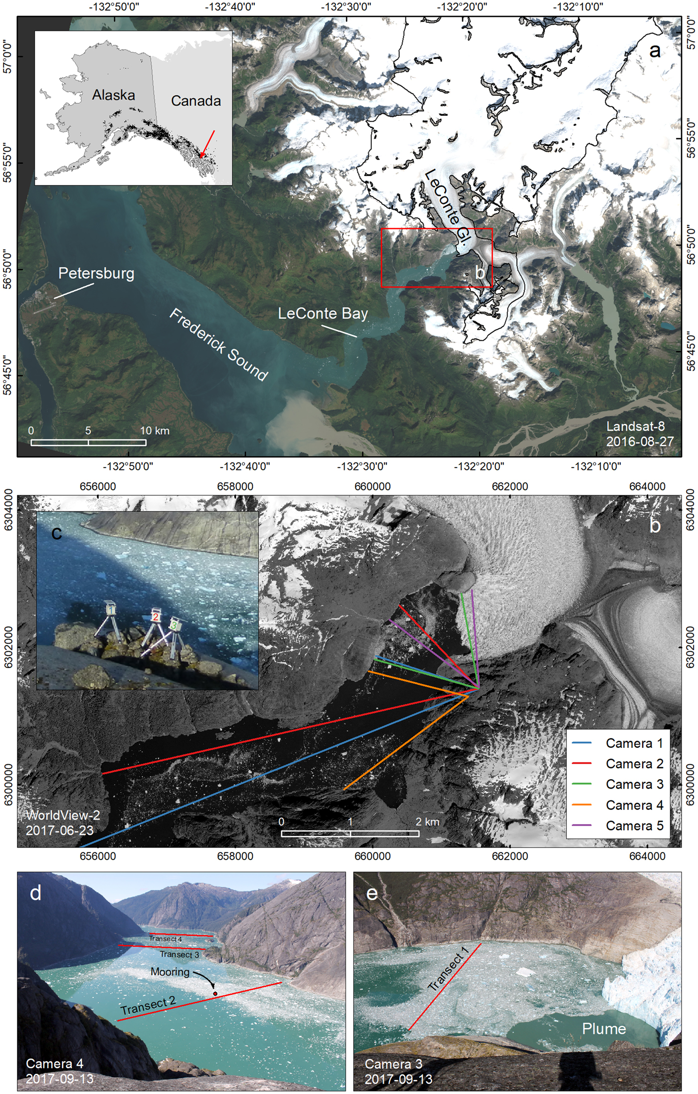
This project focuses on the innermost  $\scriptstyle \sim $6 km of LeConte Bay (Fig. 1b), where the fjord is $\scriptstyle \sim $900–1500 m wide and surrounded by steep granitic walls. Multibeam sonar measurements from 2016 yield water depths up to 320 m and an average depth of 170 m. Shallow fjord portions are rare, with only 12% of the area less than 50 m deep. The fjord is surrounded by the Stikine-LeConte Wilderness, which puts constraints on the field experiment design. For example, deployment of Ground Control Point (GCP) markers for camera model calibration was not permitted.
3. DATA
3.1. Time-lapse imagery
We ran up to five time-lapse cameras simultaneously. The cameras were placed on granitic bedrock  $\scriptstyle \sim $420 m above LeConte Bay, using surveying tripods (Figs 1b, c). We deployed four Harbortronics Time-Lapse Camera Packages with 18 mm Canon Rebel T3 or T5 single-lens reflex (SLR) cameras (www.harbortronics.com/Products/TimeLapsePackage, Table 1). These time-lapse systems consume minimal power, recharge via solar panels and have flexible programming modes. A fifth system was custom-built with a 28 mm Canon EOS 50D SLR camera. Cameras 1–3 were co-located within a radius of $\scriptstyle \sim $5 m (Fig. 1c) and deployed for 18 months (April 2016–September 2017), at frame rates of 0.5 min−1. Camera 4, located $\scriptstyle \sim $200 m to the southwest of cameras 1–3, was deployed from April to September 2017 at a frame rate of 1 min−1. The custom-built camera 5 was placed 25 m to the northeast of cameras 1–3 and deployed at a frame rate of 4 min−1 during three field campaigns (April, May and September 2017, 2 weeks in total). We refer to cameras 1–4 as ‘low-rate’ cameras, and camera 5 as the ‘high-rate’ camera. Overall, the cameras took imagery 6–12 hours per day (depending on daylight availability), capturing a total of 410 000 images.
Key properties of the time-lapse cameras used in this study. Horizontal coordinates are in the WGS84 UTM coordinate system (zone 8). Elevation is measured relative to the WGS84 ellipsoid. Azimuths, measured clockwise from North, indicate the camera's approximate look direction
We surveyed camera locations with a geodetic-quality GPS (Trimble NetRS) and measured camera rotation angles to provide initial estimates for camera model calibration. To quantify clock drift, we took photos of a handheld GPS or GPS watch (e.g., Garmin GPSMAP, Garmin Forerunner) while servicing the cameras, which we did every 1--6 months. To prevent power outages, we connected external batteries to the time-lapse systems over winter.
Unlike previous projects, where the frame rate was constrained by storage card or film capacity, mechanical failure of the camera shutters was our key consideration in this project. While the Rebel T3 and T5 cameras lack official shutter durability ratings, online sources list shutter durabilities in the 50 000–100 000 frame range. We therefore limited the maximum frame numbers to 100 000 per camera. For the low rate cameras, 256 GB Secure Digital (SD) storage cards allowed us to shoot at the highest possible image resolutions (Table 1), yielding image sizes between 5 and 10 MB in .jpg format.
None of the shutters failed during deployment, but we experienced problems with other elements of our time-lapse systems. Most notably, two cameras began to fail to save pictures several weeks after being serviced, apparently at random. They eventually stopped saving pictures completely though their shutters were still triggered. Storage cards and timers showed no damage, identifying camera-related problems beyond shutter failure as potential causes of this behavior. Additional data gaps occurred due to poor weather, namely snow and fog, that obscured the view of the bay.
3.2 ADCP data
We collected ADCP data from ships and moorings. For the shipborne measurements, we mounted a 600 kHz Teledyne RDI ADCP (depth range 4–60 m, vertical resolution 2 m) on the gunwale of an 8 m landing craft. The vessel traveled slowly along transect 2 (Figs 1d, 2a), taking one ADCP measurement per second. Onboard GPS provided vessel position, drift, and orientation in real-time. Completion of each transect survey took 1–1.5 hours typically. Icebergs and currents caused the vessel position to deviate up to 200 m from the original transect; occasionally, the transects could not be completed due to icebergs. Overall, we used 20 transect surveys from 2016 (9–15 August) and 12 from 2017 (10–13 July), all of which overlap with imagery from cameras 1 and 2. Four surveys from July 2017 also overlap with footage from camera 4. Figure 2b illustrates the average currents measured over the 32 transect surveys.
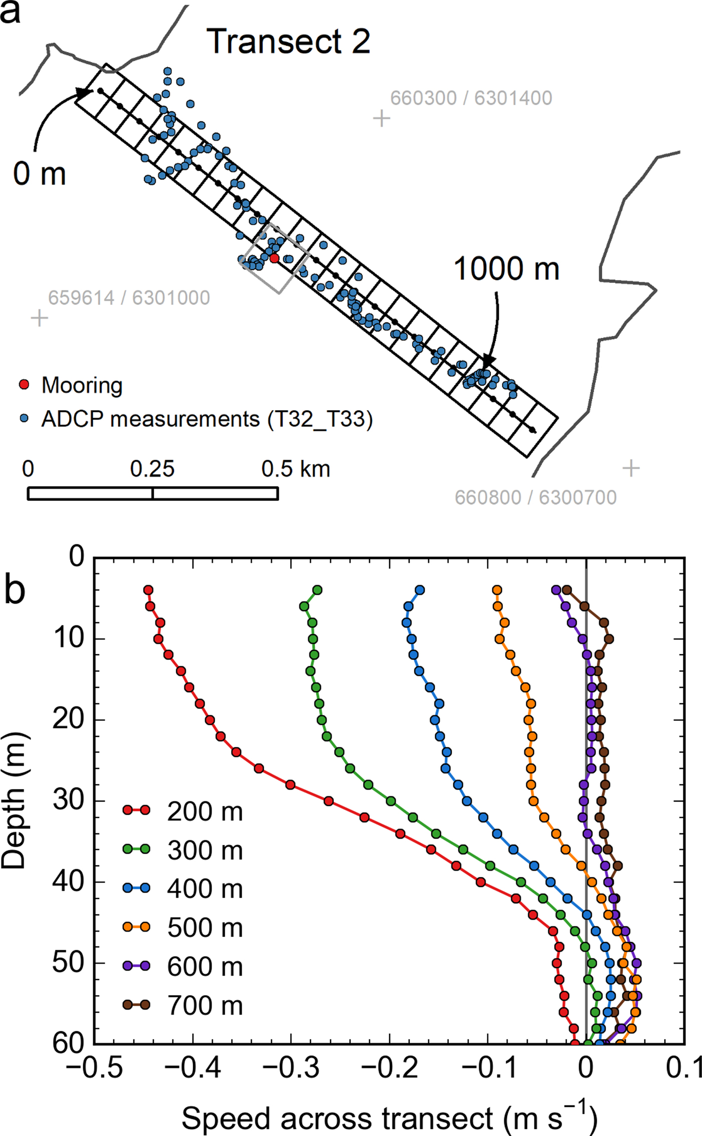
(a) Map view of transect 2. The transverse coordinate's origin (labeled ‘0 m’) is located at the north end of the transect. Blue dots show the location of selected shipborne ADCP measurements (30 s averages from survey T32_T33, Fig. 8c). The grid along the transect reflects the  $50\, {{\rm m}} \times 100\,{\rm m}$ grid used for spatial aggregation of velocity measurements. The red dot shows the mooring's location at $\scriptstyle \sim $475 m transect distance, including $100\, {{\rm m}} \times 100\,{\rm m}$ grid (gray square) used for spatial aggregation of image-derived velocity measurements. (b) Shipborne ADCP-derived speeds at six locations along transect 2,per 2 m depth levels, over the depth range 4–60 m. Speeds reflect averages over the 32 transect surveys taken in August 2016 and July 2017. They are perpendicular to transect 2 with negative speeds indicating downfjord flow and positive speeds upfjord flow. Note the signature of the outflowing plume at the 200–400 m transect locations, with strong downfjord flow above 30–40 m water depth.
An upward looking, mooring-mounted 300 kHz Teledyne RDI ADCP was deployed from May to September 2017 near transect 2 (Figs 1d, 2). Located at  $\scriptstyle \sim $100 m depth, it recorded velocities every 30 seconds at 4 m vertical resolution. Measurements for the 4 and 8 m depth levels were discarded due to side lobe contamination. Following collision with an iceberg on 26 August 2017, the mooring lost its top floats, which caused the mooring line and attached instruments to fall and cover the ADCP. Here, we use velocity data from 10 May to 25 August only. Up to three cameras (1, 2, 4) took photos of the mooring location during this time. Overall, there is more than 600 hours of overlap between the two datasets. Figure S1 shows the corresponding ADCP-derived currents.
4. METHODS
4.1. Image processing
The image processing aims to derive iceberg velocity fields in map coordinates. We first determine displacements on the oblique photos with OpenCV's Shi-Tomasi corner detector and Lucas-Kanade sparse optical flow tracking algorithms. Using a calibrated camera model, we then project the trajectories from image coordinates to map coordinates. Finally, we filter implausible displacements and average the remaining displacements over space and time.
OpenCV (https://www.opencv.org), written in C++, is at the core of the tracking portion of our code, while the remaining code (camera model, postprocessing) is written in Python. The code can be run in parallel to improve processing performance. Processing the entire dataset takes about one week on a Linux workstation with ten Intel i7 cores, 128 GB RAM, and a dedicated 1 TB solid state drive.
The following sections provide background on the tracking algorithm and camera model, and then detail the key steps of our processing workflow.
4.1.1. Tracking algorithm
Icebergs are ideal visual tracers as they provide sharp contrast against the water around them. However, iceberg distribution is often irregular due to localized calving events, wind and fjord currents (buoyant objects like icebergs gather in regions of surface convergence, e.g., D'Asaro and others, Reference D'Asaro2018). Areas with numerous icebergs may occur adjacent to open water where displacement detection typically fails due to the absence of traceable features. OpenCV's implementation of sparse optical flow performs well in these conditions by deriving displacements for traceable features of interest (i.e., corners of icebergs), while refraining from tracking in areas without such features (i.e., open water). The resulting velocity fields are neither regular nor complete, however, the derived fields are typically reliable and their computation is fast. Alternative algorithms operating on regular grids tend to yield high numbers of false velocities in areas of open water. In our tests, we were unable to filter such false velocities reliably without coincidentally removing many correct tracking results.
The optical flow problem is described by an advection equation,
 $$ {\displaystyle{\partial I} \over {\partial x}} {\displaystyle{\Delta x} \over {\Delta t}} + {\displaystyle{\partial I} \over {\partial y}} {\displaystyle{\Delta y} \over {\Delta t}} = -{\displaystyle{\partial I} \over {\partial t}}, $$
where I is the intensity of an individual image pixel, x and y the image coordinates, and t the time. The two velocity components (Δx/Δt, Δy/Δt) are typically unknown, leaving Eqn (1) underdetermined. Accordingly, additional constraints are needed in order to quantify the velocities. In the case of the Lucas-Kanade method applied here (Lucas and Kanade, Reference Lucas and Kanade1981; Bouguet, Reference Bouguet2001), neighboring pixels are incorporated to convert the above underdetermined problem into an overdetermined one, which is then solved by least squares minimization. The problem is solvable only for corners, that is, features that show changes in image density in both the x and y directions (which makes the design matrix invertible). To work reliably, this approach requires all pixels around a corner to show congruent displacement. Also, this approach (and optical flow in general) is sensitive to changes in illumination between individual images, as shown by Eqn (1), which relates changes in I to displacements only. Finally, displacements between images need to be small (ideally less than one pixel), as only small displacements allow the first order Taylor expansion used for derivation of Eqn (1). For larger displacements, coarser image versions need to be produced first, using image pyramids. Solving the optical flow problem on the coarser images provides initial flow estimates, which, in an iterative fashion, are further refined on the higher-resolution image versions (Bouguet, Reference Bouguet2001). Overall, the requirements of constant illumination and small and congruent displacements stresses the importance of using high image frame rates. Note that feature tracking with the Lucas-Kanade algorithm occurs in the Lagrangian reference frame. Individual features are followed over time, that is, over multiple images in our case.
4.1.2. Camera model
Projection from two-dimensional image coordinates (u, v) to three-dimensional map coordinates (X, Y, Z) requires a mathematical camera model and a DEM of the terrain visible in the oblique photos. Camera models of different complexities exist. While the simplest models assume a perfect camera geometry, others account for imperfections such as lens distortions (e.g., Brown, Reference Brown1966). We opted for a camera model with a minimal number of free parameters (Krimmel and Rasmussen, Reference Krimmel and Rasmussen1986). With our focus on LeConte Bay, the DEM is simplified to a horizontal plane (water level) that varies in elevation with the tides.
To constrain their free parameters, camera models typically need calibration with GCPs, which are features with known map and image coordinates. We calibrated four parameters for which we had initial estimates based on field measurements: yaw, pitch, roll (describing the camera's rotation), and focal length. Given our GPS surveys, the camera's horizontal and vertical coordinates (describing translation) were known accurately and thus not calibrated.
Our permit did not allow us to deploy GCP markers in the cameras' fields of view. Deriving natural GCPs from DEMs and satellite images was not feasible, as the steep fjord walls lack features identifiable in both satellite and oblique images. We thus relied entirely on the waterline for camera calibration. In the case of LeConte Glacier, the waterline has a distinct shape, which is required for the following approach to work. Manual digitization on a WorldView-3 satellite orthoimage from 10 April 2016 provided the map view and thus X and Y coordinates of the waterline. Tide measurements at moorings and concurrent shipborne GPS surveys of the water surface provided the waterline's elevation (Z) at the time of the satellite image (Appendix A). Manual digitization of the waterline on time-lapse photos provided image coordinates (u, v) for the waterline. Through least-squares minimization, we determined the parameter combination that best projected the waterline from the image to the map space. The final RMSEs ranged between 5 and 20 m, with larger RMSEs for cameras pointing downfjord, given their flat view angle. Note that, unlike in a classic GCP-based calibration, u–v pairs from the oblique waterline did not have pre-allocated X--Y pairs on the satellite-derived waterline. Instead, the closest X--Y pairs were determined ad hoc, after the u--v pairs' projection to map coordinates.
Camera servicing and other abrupt disturbances required semi-regular recalibration of the camera models. For this, we re-digitized the waterline on a photo that was representative of the new camera orientation and for which the tide level was close to the tide level in the WorldView-3 image. We refrained from automatically correcting camera movements between subsequent images (Harrison and others, Reference Harrison, Echelmeyer, Cosgrove and Raymond1992; Messerli and Grinsted, Reference Messerli and Grinsted2015; Schwalbe and Maas, Reference Schwalbe and Maas2017), for two main reasons. Our tracking intervals are short and corresponding camera motion small, especially relative to the large iceberg displacements. Moreover, because we average velocities temporally during postprocessing, effects of camera motion tend to cancel out given their random origin (e.g., jitter motion in strong wind).
4.1.3. Workflow
Step 1 – Tracking on oblique imagery
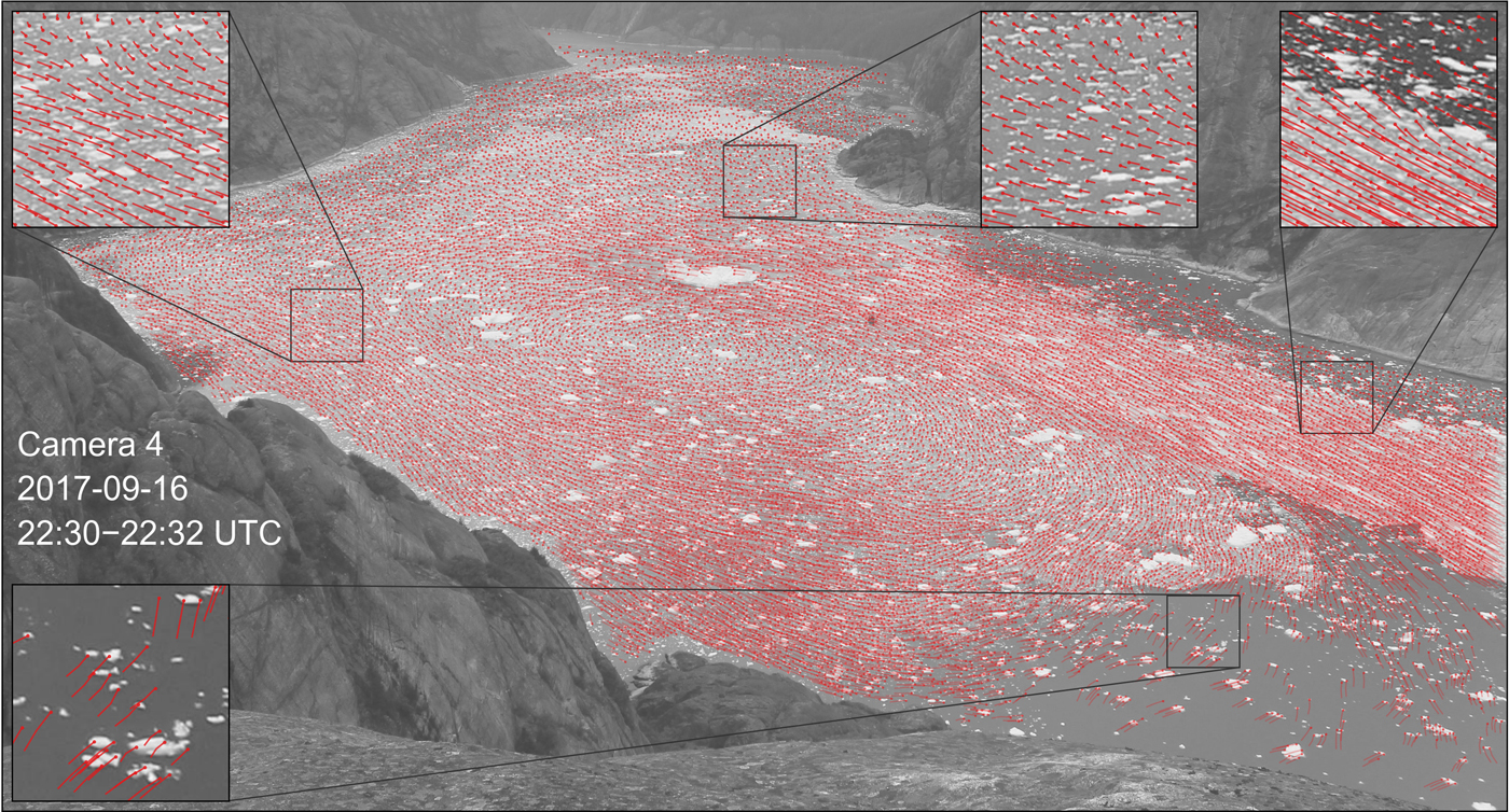
Using OpenCV's implementation of the Shi-Tomasi algorithm (Shi and Tomasi, Reference Shi and Tomasi1994), we first detect corners on grayscale versions of the original photographs. Corners are intersections of two edges, where each edge reflects a strong change in image intensity. Prior to application of the corner detector, areas outside the fjord are masked. Next, we track the corners across three subsequent images (e.g., image numbers 1–2–3), using the pyramidal Lucas-Kanade algorithm in OpenCV (Bouguet, Reference Bouguet2001). For quality control, we conduct the tracking in reverse (3–2–1) and retain only trajectories that are congruent both ways. After storing the trajectory vertices (i.e., three x--y pairs for each trajectory), we process the next image triplets (2–3–4, 3–4–5, etc.), repeating the above steps. For visual quality assessments, which are particularly meaningful in the Lagrangian reference frame, trajectories can be plotted together with the underlying imagery (Fig. 3).
Lucas-Kanade-derived trajectories (red lines) overlain on a photo from camera 4 that was used for tracking. Red dots mark the trajectories' heads. Features detected on the first image are tracked over two more photos (2 minutes in this case, since camera 4 had a frame rate of 1 min−1). Insets provide enlarged views.
The above workflow is adapted from standard computer vision workflows implemented in OpenCV. Several parameters are user-specified, for example, the minimum distance between corners (used for the Shi-Tomasi algorithm) or the maximum number of image pyramids (used for the Lucas-Kanade tracker). For a full list of parameters, refer to Table 2. We identified good parameters by visually comparing trajectories from repeat test runs and kept them constant over space and time.
User-defined parameters used during image processing. Magnitudes reflect the processing of the high-rate images from camera 5. The list excludes parameters from step 2 used for projection from image to map coordinates
*Used for the Shi-Tomasi corner detector (Shi and Tomasi, Reference Shi and Tomasi1994).
†Used for the pyramidal Lucas-Kanade feature tracker (Bouguet, Reference Bouguet2001).
‡Only applied above a speed threshold of 0.25 m s−1.
Rather than tracking over image triplets, one could track over image pairs (i.e., 1–2, 2–3, 3–4, etc.) or four or more images (e.g., 1–2–3–4, 2–3–4–5, etc.). While tracking over two images leads to the densest set of trajectories, the set may come with a relatively large number of false trajectories (partly because filtering by trajectory over multiple images is not possible). Tracking over four or more images leads to increasingly robust, yet thin velocity fields. For our photos spaced 2 minutes apart, tracking over three consecutive images was the best compromise between density of the velocity field and postprocessing options. For photos taken at higher rates, tracking over four or more images may be ideal, though this was not systematically tested.
Given the oblique camera views, pixel ground resolution differs in the horizontal and vertical domain; it also varies across-photo with distance of the imaged fjord portion from the camera. Using images with 5184 × 3456 pixel resolution (Table 1), a pixel covers 1.3 m horizontally and 17.7 m vertically at a distance of 5.5 km downfjord from camera 1. 700 m away from camera 3, a pixel has a footprint that is much smaller and less skewed, covering 0.17 m horizontally and 0.34 m vertically. Variable pixel footprints affect density of the derived corners once projected to map coordinates. They also affect the accuracy of the derived trajectories. With increasing distance from the cameras and concurrently flatter view angles, tracking accuracy declines, predominantly in the vertical direction (i.e., in up- and downfjord direction in case of camera 1).
Step 2 – Projection to map coordinates
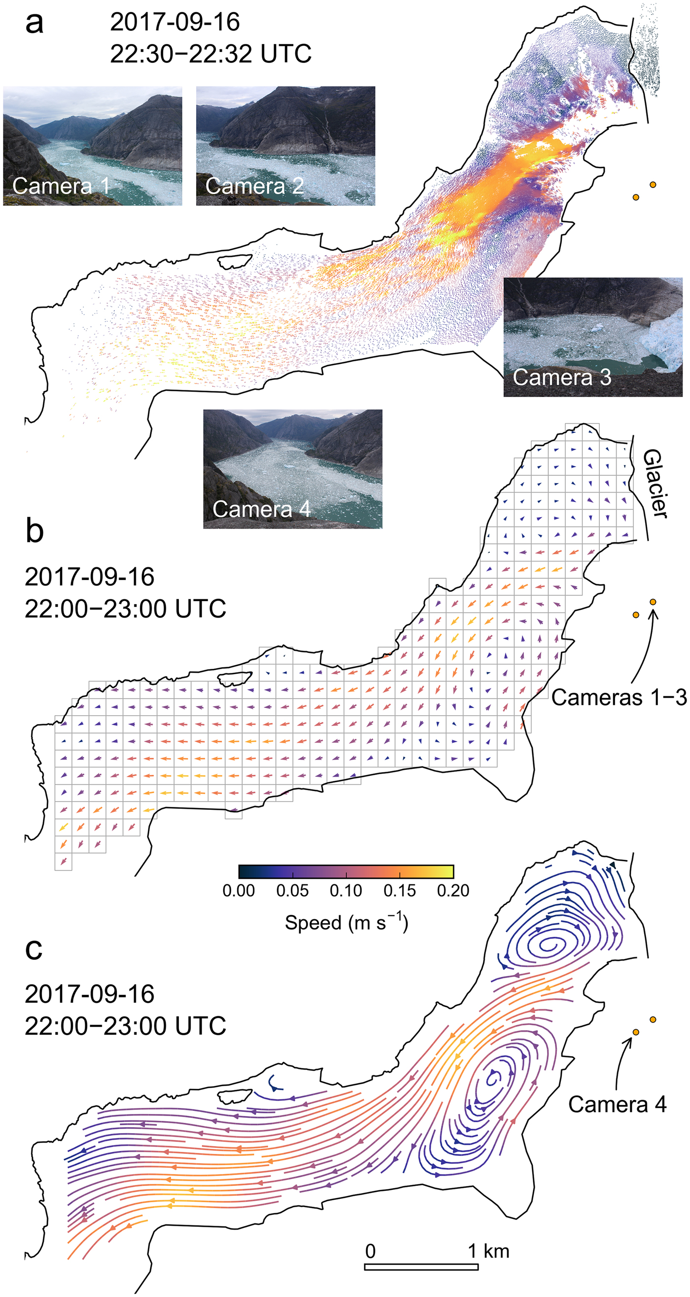
Using a calibrated camera model (Section 4.1.2), the iceberg trajectories are projected from image coordinates to map coordinates (UTM zone 8N, Fig. 4a). With the vertices in the metric UTM system and known time-lapse interval, we calculate iceberg speeds.
Key processing products. Colors represent speeds and are identical across panels. UTM-projected iceberg trajectories, including underlying photos from cameras 1–4. The trajectories represent a 2 minute interval (22:30–22:32 UTC) on 16 September 2017. Note that Fig. 3 shows the corresponding trajectories in the image coordinate system (camera 4 only). (b) Mean velocities after temporal aggregation over an hour (22:00–23:00 UTC) and spatial aggregation over a 150 m × 150 m grid. (c) Streamline plot generated from hourly averaged velocities.
For the projection, we approximate the fjord's water level by a horizontal plane that moves vertically in accordance with the tides. Tide modeling (Appendix A) provides tide elevation, and thus the elevation difference between water and camera, at 1 minute intervals. We do not account for iceberg heights, which biases vertical distances to the cameras slightly. While this causes positional errors of the trajectories and ultimately errors in speed, the errors in speed are small (1.2% in the case of a 5 m iceberg freeboard, Appendix A). Potentially larger positional errors are of limited concern, as we ultimately average the trajectories over a coarse grid (50–150 m) and because the flow field shows relatively strong spatial autocorrelation.
Step 3 – Postprocessing
Having the trajectories in the map coordinate system allows for additional filtering, conducted via absolute speed (to remove particles with implausibly high speeds), speed changes (to eliminate trajectories with implausible acceleration/deceleration), and flow direction (to remove trajectories with implausible direction changes). For simplicity, we implement discrete thresholds and discard trajectories if they exceed any of the user-specified thresholds (Table 2). Because significant speed and direction changes can be plausible at low speeds, we apply the latter criteria above a certain speed threshold only.
After filtering, we account for camera clock drift, assuming linear drift between service dates, for which we have GPS screen images. We then merge the trajectories from several cameras and aggregate them by time (i.e., hourly to daily intervals) and space (i.e., their location within a regularly spaced grid). During this step, a minimum number of trajectories can be prescribed for each group. Ultimately, statistical parameters (e.g., mean velocities) are calculated for the grouped trajectories, creating new, coarsely spaced velocity fields in the Eulerian framework (Fig. 4b). For their subsequent visual and quantitative interpretation, we use a suite of scripts, for example, to create streamline plots (Fig. 4c) or calculate flow across predefined transects.
While the final velocity fields are generally accurate, faulty trajectories may remain unfiltered, especially under foggy conditions that obscure the fjord. To mask such faulty velocity fields, we create summary figures of the hourly tracking results, which include the original photos, maps of the derived trajectories and the final averaged velocity fields. These figures are classified by an operator as trustworthy or not (blunders are typically easy to identify visually) and the resulting binary filter is applied to the velocity fields.
4.2. Uncertainty assessment
The uncertainty assessment aims at determining (1) how reliably our method captures iceberg velocities and (2) how well and over what depth range the iceberg velocities reflect fjord currents. For (1), we compare spatially and temporally overlapping velocity fields from low-rate cameras, specifically cameras 1 and 4. In addition, we use high-rate camera 5 to simulate a range of time-lapse settings, with a focus on time-lapse interval and image resolution. For (2), we compare the camera-derived velocities to ADCP measurements from vessels and moorings. Constrained by data availability and computational processing demands, the analyses cover periods ranging from hours to months.
4.2.1. Low-rate camera intercomparisons
Comparison of velocity fields from different cameras reveals differences due to camera configuration (e.g., frame rate, location, sensor properties) and camera model calibration. Because we apply the same tracking algorithm throughout the comparisons, potential algorithm-specific limitations are not captured. Our comparison focuses on cameras 1 and 4, which ran simultaneously in April 2017 and July–August 2017, over a total of 35 days. The different sampling rates, locations and sensor properties of the cameras (Table 1) make them the best choice for comparison. The velocities of camera 4 may serve as a benchmark, given the camera's higher frame rate and better field of view (steeper view angle).
We compare the velocities across transects 2–4 (Fig. 1d). To arrive at interpretable results, spatial and temporal aggregation of the original trajectories is required. To aggregate the trajectories spatially, we establish grids with  $50\, {{\rm m}}\times 100\,{\rm m}$ cell size along the three transects (Fig. 2). Temporally, we aggregate over 2 hour periods. For the aggregated trajectories, we calculate iceberg speeds perpendicular to the course of the transects, which facilitates subsequent comparisons (two-dimensional velocities are reduced to speeds) without losing critical information. Ultimately, we compare the results (i.e., 25th quantiles, medians, 75th quantiles) from the two cameras visually and quantitatively (through scatterplots and linear regression).
The choice of time periods and areas used for temporal and spatial aggregation is a compromise between too short/small (too few measurements) and too long/large (loss of relevant information). Tests suggested 2 hour periods and 50 m × 100 m grids as a good compromise. For consistency, we use these exact or similar parameters throughout all our assessments, including camera to ADCP comparisons.
4.2.2. High-rate camera simulations
The low-rate camera comparisons are useful for assessing agreement among velocity fields from different cameras. Identifying the underlying causes of these differences, however, may be speculative, as the cameras differ in several properties, which may all affect the results. Using one camera to simulate different time-lapse settings avoids this problem, as the settings (e.g., frame rate) can be changed individually. High-rate camera 5 is ideal for such simulations because it sampled at a rate of 4 min−1 and captured the dynamic portion of the fjord close to the glacier face, where strong currents occur due to plume dynamics and calving activity.
We here vary two properties: time-lapse interval (15–240 s) and spatial resolution of the input images (40–100% scaling). For each spacing/resolution combination, we run the full image processing workflow (Section 4.1.3). To reduce computational and data storage demands, we focus on a 4 hour period deemed representative of summer conditions. We chose a period on 11 May 2017 (22:00–02:00 UTC) that featured strong currents in the outflowing plume, occasional calving events, and generally favorable weather for tracking (overcast with brief periods of sunshine). To assess the simulation results, we compare velocity fields from different scenarios visually. In addition, we compare speeds across transect 1 (Fig. 1e) quantitatively, using the approach introduced in Section 4.2.1.
4.2.3. Comparison with shipborne ADCP measurements
To assess the agreement of iceberg velocities and actual near-surface currents, we compare our image-derived velocities with concurrent shipborne ADCP data (Section 3.2). From the ADCP data, we use the uppermost 11 depth levels, representing 2 m bins between 4 and 24 m water depth. Incorporating several depth levels allows us to evaluate whether the match between image- and ADCP-derived velocities varies with depth.
We aggregate the image- and ADCP-derived velocities by space and time. Given their sparseness, we include all ADCP-derived velocities regardless of their lateral distance from the transect, while considering image-derived velocities detected within 50 m × 100 m grid cells (Fig. 2). For temporal boundaries, we include all image-derived velocities detected within 1 hour of the ADCP survey's halftime, yielding a 2 hour period in total. For the aggregated velocities, we compute speeds across transect 2 and compare the corresponding statistics (25th quantiles, medians, 75th quantiles) visually and quantitatively.
4.2.4. Comparison with mooring ADCP measurements
Comparing our image-derived velocities to velocities from the mooring-mounted ADCP allows us to extend the comparison period to several weeks and additional depth levels. For the comparison, we select image-derived trajectories within a 100 m × 100 m grid cell centered at the mooring location and rotated parallel to transect 2 (Fig. 2). Following the above comparisons' methodology, we compare speeds perpendicular to the course of transect 2, temporally aggregated over 2 hour periods. We also compare the actual flow azimuths, which provides additional insights into the agreement of the two datasets.
5. RESULTS AND DISCUSSION
5.1. Uncertainty assessment
5.1.1. Low-rate camera intercomparisons
A wide range of ice and current conditions prevailed during the 35 day comparison. In early April 2017, the fjord was choked with ice, while only a few icebergs were present in July 2017. Overall, currents were predominantly downfjord, as indicated by mostly negative speeds across the transects (Fig. 5).
(a–i) Camera 1-derived speeds (0.5 min−1 frame rate) vs camera 4-derived speeds (1 min−1 frame rate) measured along transect 2, for 9 selected days (Fig. S2 features additional days). Each panel represents the 20:00–22:00 UTC time period for 1 day. The inset images taken from camera 4 show the fjord at 21:00. Abscissas reflect distance along the transect and ordinates speed perpendicular to the transect (negative speeds indicate downfjord flow). Dots describe the median speeds per 50 m bin; error bars represent the corresponding first and third quartiles. For better readability, the dots are shifted slightly to the right (camera 1) and to the left (camera 4). (k) Scatterplot comparing camera 1- and camera 4-derived speeds including statistical parameters. The dots represent median speeds per 50 m bin; r and ‘mae’ correspond to the correlation coefficient and mean absolute error, respectively.
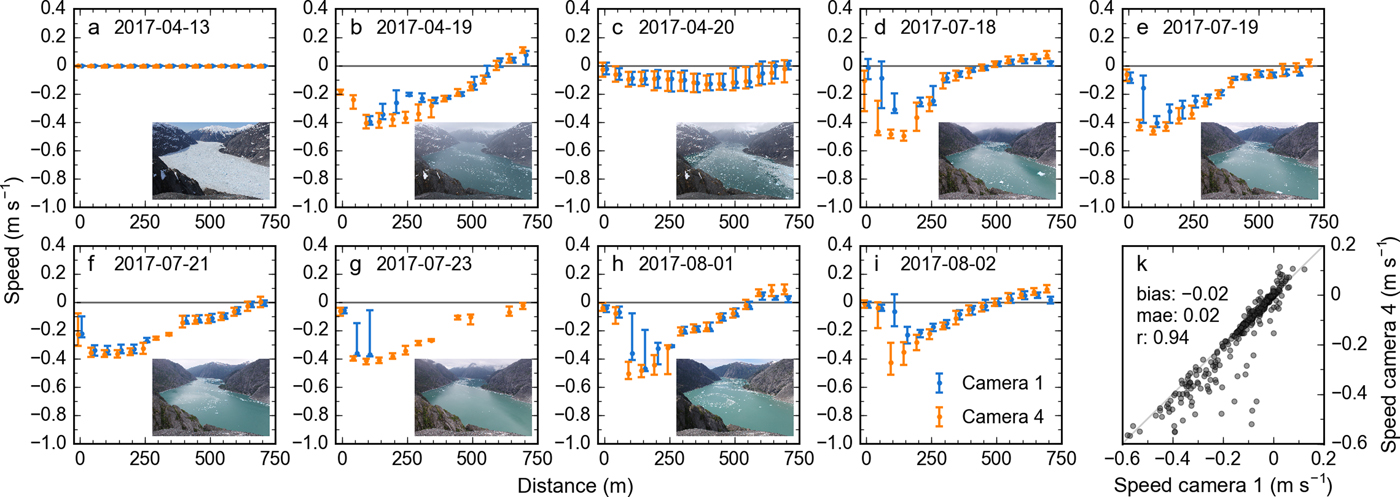
Generally, we find good agreement among the speeds derived from cameras 1 and 4. For transect 2 (Fig. 5, Table 3), comparison of the two datasets yields a mean absolute error (mae) of 0.02 m s−1 and a bias of –0.02 m s−1 (camera 4 more negative). Moreover, the speed datasets capture 88% of each other's variability (r 2 = 0.88, p < 0.01). In the case of abundant icebergs and low speeds (e.g., on 20 April 2017, Fig. 5c), the speeds from the two cameras are essentially identical. However, camera 4 outperforms camera 1 when iceberg speeds are high (e.g., on 18 July 2017, Fig. 5d), as illustrated by fewer measurement gaps, fewer outliers, and smaller error bars. In the case of the highest iceberg speeds (between –0.4 and –0.6 m s−1), camera 4 provides speeds that are higher and more consistent than those from camera 1 (note the increasing number of outliers for camera 1 in Fig. 5k). In these cases, camera 1 (0.5 min−1 sampling rate) likely misses more of the fastest icebergs, which results in median velocities lower than those from camera 4 (1 min−1 sampling rate). The fact that camera 4 detects three times more trajectories, with only double the sampling rate, supports this conclusion. For reference, the comparison between cameras 1 and 2 (rather than 4) at transect 2 yields an r 2 of 0.96 and a 0 m s−1 bias (Table 3, Fig. S3). This better agreement is likely explained by the two cameras' similar configurations (i.e., identical sampling rates and sensor properties, and essentially identical locations, Table 1) and suggests consistent calibration of the camera models.
Statistical parameters derived from low-rate camera intercomparisons along transects 2–4. r is the correlation coefficient and ‘mae’ corresponds to the mean absolute error
Along transects 3 and 4, the agreement between speeds derived from cameras 1 and 4 is excellent, with r 2 values of 0.96 and zero biases (Table 3, Figs S4, S5). Speeds across transects 3 and 4 are generally lower than those at transect 2, facilitating the tracking task. Additionally, transects 3 and 4 lie downfjord from transect 2 and thus farther away from the cameras, where moving icebergs cause smaller displacements on the photos. Lower iceberg speeds in the fjord and smaller displacements on the photos may benefit camera 1 (0.5 min−1 sampling rate) more than camera 4 (1 min−1 sampling rate), explaining the improved performance of camera 1 relative to camera 4. While tracking tends to become more robust with increasing distance from the cameras, potential tracking accuracy decreases, especially with flattening view angles. Because we use one common tracking algorithm and cameras with similar view geometries (with respect to transects 3 and 4), our comparison likely fails to describe decreasing tracking accuracy, which needs to be borne in mind for future analyses.
Overall, this comparison confirms the advantage of using high frame rates, especially for areas close to the cameras and subject to high iceberg speeds. With higher frame rates, both iceberg displacements and lighting changes decrease, which facilitates tracking by means of optical flow.
5.1.2. High-rate camera simulations
Our simulations with high-rate camera 5 on 11 May 2017 capture the fjord in a dynamic state. A strong outflowing plume was present on the south side of the fjord, with iceberg speeds up to 1 m s−1. To the north of the plume, a clockwise rotating eddy was present, mostly with iceberg speeds between 0.1 and 0.3 m s−1. Intermittent calving events caused very fast ice movement.
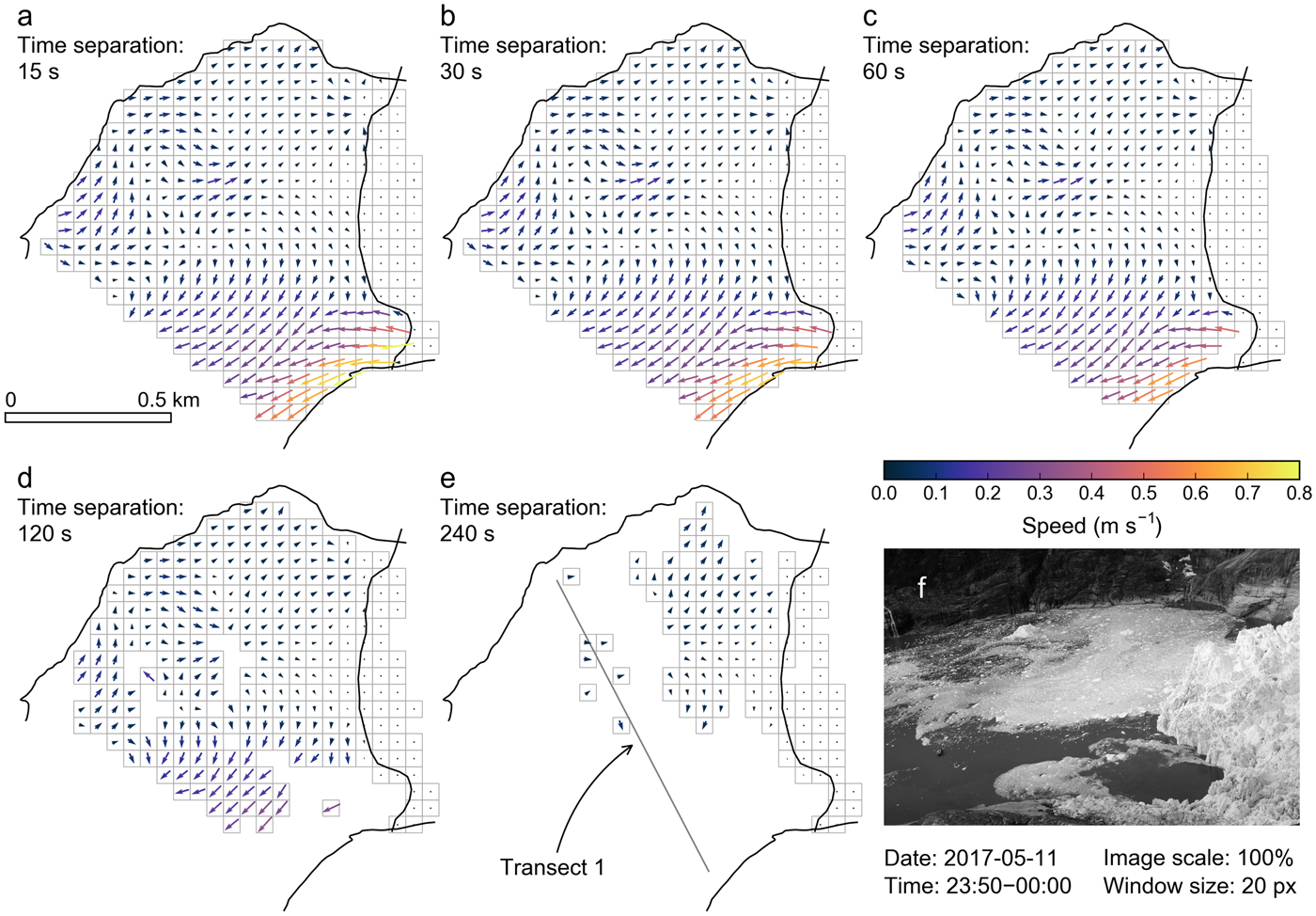
Simulations with five time-lapse intervals (15, 30, 60, 120 and 240 s, corresponding to frame rates of 4, 2, 1, 0.5 and 0.25 min−1) yield velocity fields with markedly different degrees of completeness (Fig. 6). The velocity fields from the 15 s scenario show the most comprehensive fjord coverage (Fig. 6a). Visual comparison of the original trajectories to their underlying oblique photos confirms best tracking performance on images spaced 15 s apart. We find no obvious change in the velocity fields when decreasing the time-lapse interval to 30 s, except in the immediate plume area, which occurs because the algorithm begins to miss the fastest icebergs (Fig. 6b). The velocity field completeness begins to decline with the 60 s scenario, first across the plume (Figs 6c, d) and then across the remainder of the fjord (Fig. 6e). Although scenarios with lower frame rates provide partial velocity fields only, the remaining portions appear valid overall, especially when averaged over extended time periods (e.g., 1 hour rather than 10 minutes, Fig. S6).
Results from simulation runs at camera 5, varying the time-lapse interval from (a) 15 s to (e) 240 s. The velocity fields reflect averages over 10 minutes (here 23:50–00:00 UTC) and a 50 m × 50 m grid. Panel (e) includes the location of transect 1, used for quantitative assessment of simulation results (Fig. 7). The photograph in panel (f), captured by camera 5, shows the fjord at 23:50 UTC.
(a–d) Speeds from four time-lapse interval scenarios (30–240 s) vs speeds from the reference scenario (15 s time separation). Dots represent hourly median speeds perpendicular to transect 1, per 50 m × 100 m grid cell. n reflects the total number of measurements compared, 84 being the maximum (4 hours × 21 grid cells). The red line represents the linear fit to the data, with magnitude of slope and intercept annotated in the panel. The gray line is the 1:1 line. Note that the zero biases in panels (b)–(d) result from mutual compensation of underestimated downfjord and upfjord flow.
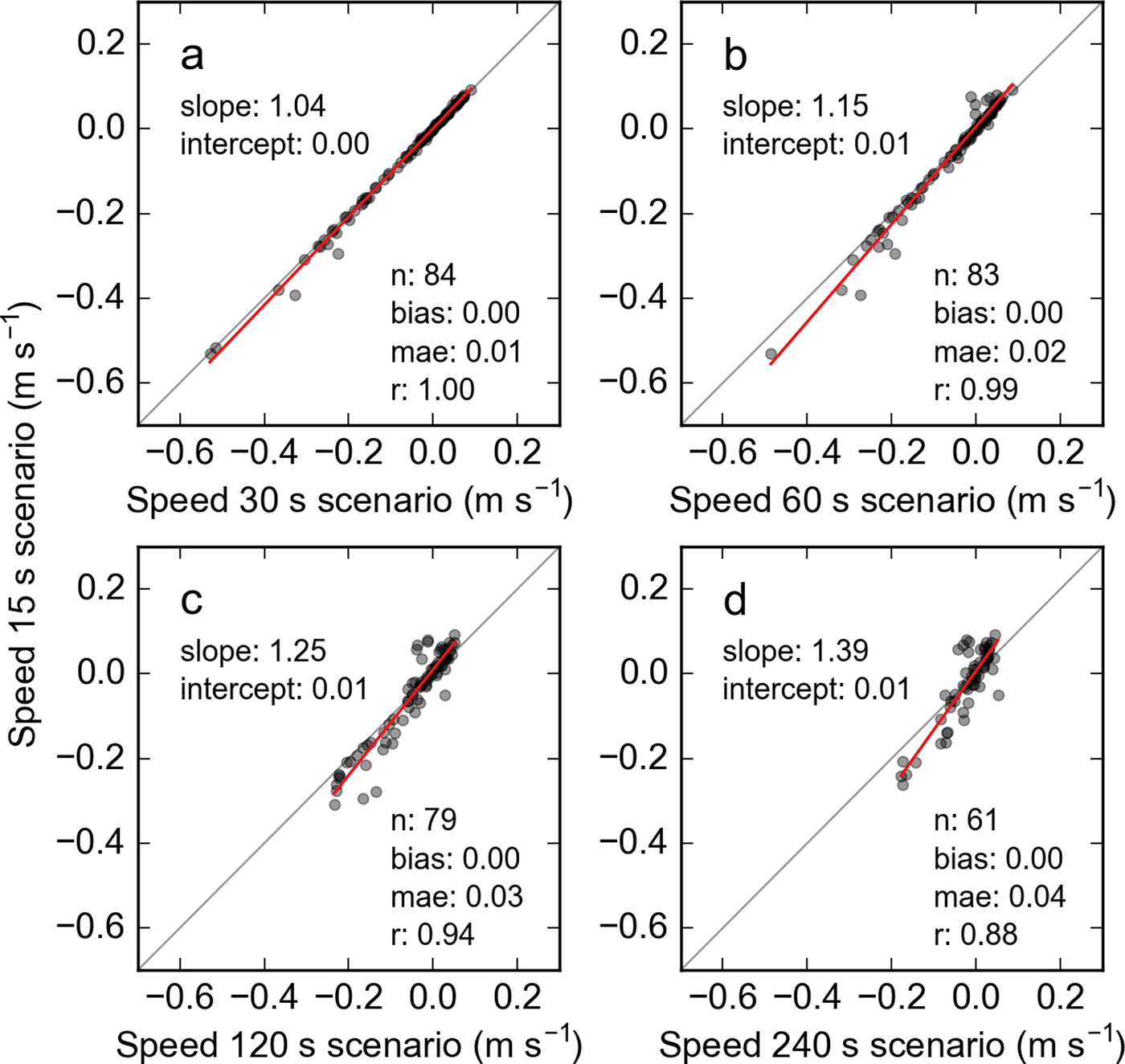
Quantitative comparison of speeds across transect 1 confirms the findings from the visual analysis and supports results from Section 5.1.1 regarding biases in the velocities from low-rate cameras. While the speeds from the 30 and 15 s scenarios are nearly identical (Fig. 7a), fast flow tends to be underestimated towards sparser time-lapse intervals (Figs 7b–d). The highest downfjord speeds (approximately −0.5 m s−1) are missed entirely in the 120 and 240 s scenarios. Underestimation scales with time-lapse interval, as indicated by increasing slopes of the linear fits in Fig. 7.
Simulations with different resolution input images (100, 80, 60 and 40% of the original size) yield nearly identical velocity fields (Fig. S7). Even with input images that are 40% of the dimension of the original image, the tracking results show minimal change. This is likely related to the very high resolution of our original photographs, 4752 × 3168 pixels in the case of camera 5. In the area of the plume, this corresponds to a ground-resolution of  $\scriptstyle \sim $20 cm. Hence, even small iceberg displacements exceed several pixels in the original images, which are handled by the Lucas-Kanade tracker through image pyramids (reduced size versions of the original image, Section 4.1.1) and potential additional smoothing of the input imagery. Although the Lucas-Kanade tracker refines the final displacements with the highest resolution image version, these corrections must be small in our case. Hence, for tracking purposes, reduced size images may be sufficient, especially if the perimeter covered is close to the camera.
Overall, these simulations confirm frame rates as the key factor affecting tracking results. High frame rates are particularly important in the case of high/divergent iceberg speeds and rapid changes in lighting conditions. For settings similar to those at LeConte Glacier, 15–30 s time separation are required for best tracking results. Sixty second time separation still provides good velocity fields, though with occasional gaps and potential underestimation of high speeds. The maximum legitimate time separation is 120 s, although the resulting velocity fields miss the fastest portion of the plume and may underestimate higher speeds in general.
When using high-resolution cameras similar to ours (Table 1), image resolution can be reduced by 50% without notable losses in the quality of the velocity fields. Reducing the image size by half allows for increasing the frame rate by about a factor of 4 (if the frame rate is limited by storage space). However, note that spatial resolution may remain important for camera model calibration by simplifying identification of GCPs.
5.1.3. Comparison with shipborne ADCP measurements
For both campaigns (August 2016 and July 2017), ADCP measurements show fast downfjord speeds in the northern portion of transect 2, reaching from the water surface to 30–40 m depth (Fig. 2b). At 200 m transect distance, downfjord velocities exceed 0.4 m s−1 above 20 m depth (average over 32 transect surveys), reaching up to 0.6 m s−1 during selected transect surveys. These downfjord speeds at shallow depths abate toward the southern portion of the transect and beyond  $\scriptstyle \sim $600 m, flow is predominantly towards the glacier. This pattern reflects the outflowing plume and an adjacent eddy with counterflow. Counterflow is also observed beyond 40–50 m water depth. Speed patterns are similar across the 11 ADCP levels used for this comparison (4–24 m), though magnitudes tend to decrease with depth. Here we illustrate the comparison with the 6 m ADCP measurements (Fig. 8); comparisons to other depth levels yield similarly looking figures (Figs S8–S11).
(a–f) Image- vs 6 m ADCP-derived speeds along transect 2. Each panel shows one ADCP survey with corresponding speeds derived from cameras 1 and 2 (a–e) and 1, 2 and 4 (f). Panels (a–c) represent three selected surveys from the August 2016 campaign, (d–f) three selected surveys from the July 2017 campaign. Inset images taken from camera 1 show fjord conditions halfway through the ADCP survey. Times show the start and completion times of the ADCP surveys. Gray dots show individual ADCP measurements. Green and blue dots describe median speeds per 50 m × 100 m bin; corresponding error bars show the first and third quartiles. For better readability, dots and error bars are shifted slightly to the left (ADCP-derived speeds) and to the right (image-derived speeds). Areas beyond 700 m (gray vertical line) are only visible from camera 4, which was operational only during ADCP surveys on 13 July 2017. (g) ADCP- vs image-derived speeds, with corresponding statistical parameters. Semi-transparent black dots represent median speeds per 50 m × 100 m bin, collected from 32 ADCP surveys. Red dots indicate outliers caused by two icebergs stranded on 12 and 14 August 2016, yielding image-derived speeds of zero. The gray line is the 1:1 line.
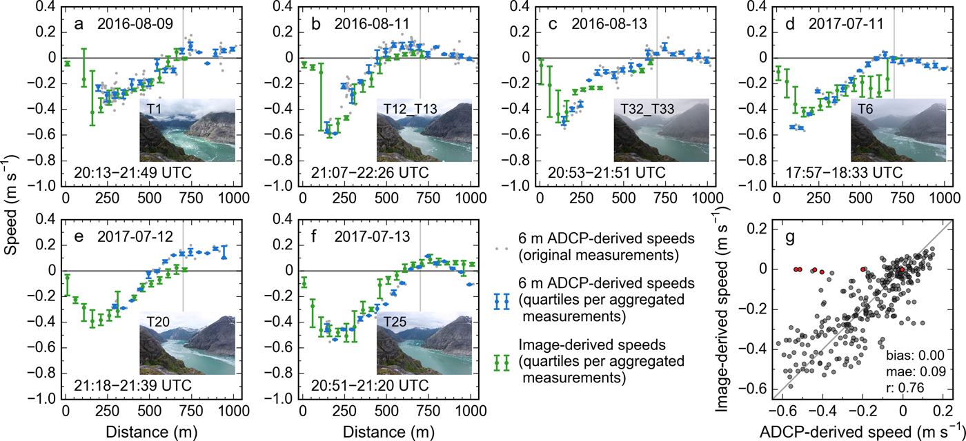
Overall, our image-derived speeds capture the speed patterns by the ADCP well, including peak speed at  $\scriptstyle \sim $200 m transect distance and decreasing speeds towards the southern transect portion (Figs 8a–f). In fjord portions with dense ice cover (inaccessible by vessel), the image-derived speeds actually extend the ADCP-derived measurements. Quantitative comparison of image- and ADCP-derived speeds confirms a statistically significant correlation (e.g., r = 0.76 for the 6 m ADCP-derived speeds, Fig. 8g). While biases are zero for the shallowest depth levels (4–8 m), they increase beyond 8 m, along with increasing mean absolute errors and decreasing correlation coefficients (Table 4). Despite the good overall match, scatter is considerable, indicated by mean absolute errors of at least 0.09 m s−1. At low speeds, relative errors can exceed 100%, which needs to be borne in mind especially when interpreting individual measurements (relative errors increase towards lower speeds although absolute errors tend to decrease).
Statistical parameters derived from the comparison between image-derived and shipborne ADCP-derived speeds, for 11 ADCP depth levels at transect 2. The speeds compared are perpendicular to transect 2. Negative biases indicate that the image-derived speeds are faster than the ADCP-derived speeds
Several outliers show image-derived speeds of zero while concurrent ADCP-derived speeds are relatively high (red dots in Fig. 8g). Inspection of time-lapse images indicates that these zero velocities are not due to tracking errors, but to two large icebergs stranded in the shallow portion of transect 2 (between 0 and 150 m, at water depths < 30 m). Note that stranded icebergs are not generally a problem in LeConte Bay. Indeed, the above comparison with ADCP data suggests that most of the tracked icebergs have keel depths shallower than  $\scriptstyle \sim $10–12 m, which agrees with field observations. Most icebergs observed are only a few meters in width and stability considerations suggest that icebergs tend to be shallower than they are wide (e.g., Wagner and others, Reference Wagner, Stern, Dell and Eisenman2017).
5.1.4. Comparison with mooring ADCP measurements
Over this long-term comparison (10 May–25 August 2017), the ADCP-derived speeds (2 hour averages, perpendicular to transect 2) are predominantly negative at shallow depths (above  $\scriptstyle \sim $40 m), indicating downfjord currents. Speeds reach up to –0.35 m s−1 at the 12–16 m depth levels (mean speeds = –0.08 m s−1, Fig. S1) and generally decrease with depth, similar to observations from previous comparisons. The 40 m depth level marks the transition zone where both downfjord and upfjord flow occur (Fig. S1). At depths below $\scriptstyle \sim $48 m, flow is predominantly upfjord.
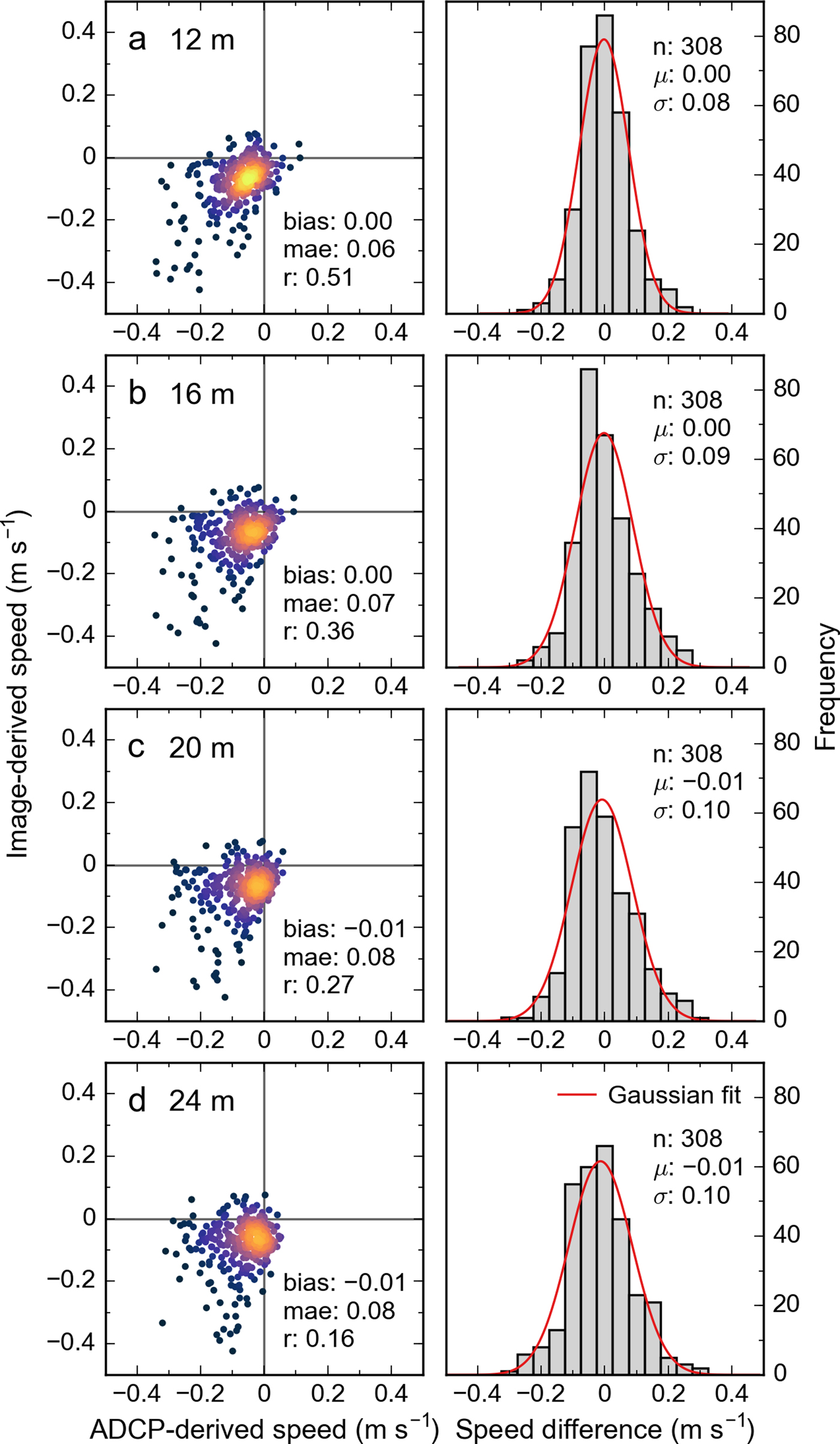
Despite considerable scatter, there is a significant positive correlation between the image- and ADCP-derived speeds for the uppermost depth levels (Fig. 9, Table 5). The correlation is highest for the 12 m depth level, where the image-derived speeds explain 26% of the variability in the ADCP-derived speeds (r = 0.51, p < 0.01). The correlation declines with ADCP depth level, reaching an r value of 0.16 at 24 m. Beyond 24 m, correlations lose significance (p > 0.01) temporarily (Fig. S12). Significant (though weak) negative correlation starts at 48 m depth, implying that increasing downfjord speeds at the surface correlate with increasing upfjord speeds at depth.
(a–d) Comparison of image-derived velocities (from cameras 1, 2 and 4) and corresponding mooring-mounted ADCP measurements for depth levels 12, 16, 20 and 24 m. Each of the 308 measurements represents a 2 hour period between 10 May and 25 August 2017. Scatterplots (left panels) compare the speeds measured at the annotated mooring depths to the image-derived speeds. Speeds are perpendicular to transect 2, with negative values indicating downfjord flow. Colors represent point density, with lighter colors indicating higher numbers of overlapping points. Histograms (right panels) show the corresponding frequency distributions of speed differences (image-derived speeds – ADCP-derived speeds), including Gaussian fits. Bin size is 0.05 m s−1. μ and σ values represent means and standard deviations. Note that the 12 m depth level features the most favorable error distribution. A figure with additional depth levels is given in the Supplementary Material (Fig. S12).
Statistical parameters derived from the comparison between image-derived speeds and speeds from the mooring-mounted ADCP. The speeds compared are perpendicular to the course of transect 2. The comparison covers eight ADCP depth levels. ‘n.s.’ marks non-significant correlations. Figs 9 and S12 shows the corresponding scatterplots
The highest correlation for the 12 m depth level coincides with the smallest bias and mae values (0 and 0.06 m s−1, Table 5), identifying 12 m as the best matching depth level. Analyzing the actual distributions of speed differences (histograms in Fig. 9) yields the most favorable error distribution for the 12 m depth level, supporting this finding. Note that the speed differences follow Gaussian distributions closely, which is expected given many (random) error sources affecting the two velocities compared (see next section).
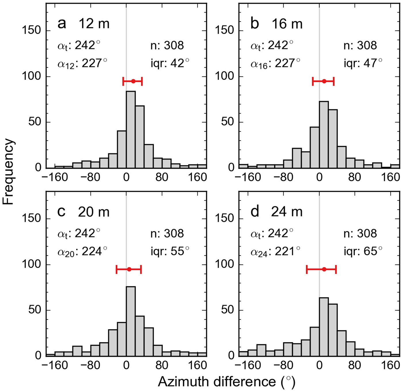
In line with the previous observations, the flow azimuths of image- and mooring-derived velocities show the best agreement for the shallowest depths (Fig. 10). Interestingly, the average azimuths are shifted by  $\scriptstyle \sim $15°, indicating that the image-derived azimuths point in a more westerly direction than the mooring-derived azimuths. This difference likely quantifies azimuthal change in the unmeasured currents above 12 m depth, which are a key control on the predominantly small icebergs in LeConte Bay. Due to the 15° azimuth difference, the ADCP-derived velocities pass transect 2 more orthogonally than the corresponding image-derived velocities, which affects the projected speeds analyzed in Fig. 9 and Table 5. Upon projection of same-magnitude velocities, the 15° azimuth difference causes an artificial speed difference of 8%, underestimating the image-derived speeds relative to the ADCP-derived speeds. In the case of the 12 m depth level, considering this difference yields a speed bias of –0.01 m s−1 rather than the 0.0 m s−1 given in Table 5. This negative bias is plausible as the downfjord currents above 12 m water depth (which control small icebergs) tend to be stronger than those at 12 m (Fig. 2b).
(a–d) Same as Fig. 9, but showing frequency distributions of azimuth differences (azimuth of image-derived velocity – azimuth of ADCP-derived velocity at annotated depth). Average north-based azimuths are annotated for the observations compared, with αt reflecting iceberg tracking-derived azimuths and α12–α24 ADCP-derived azimuths. Red error bars indicate the distributions' three quartiles; the interquartile range is also annotated as ‘iqr’. Quantiles are chosen given the distributions’ non-Gaussian shape.
5.1.5. Agreement of iceberg speeds and fjord currents
Our assessments suggest the best agreement (smallest biases, smallest mae values) for the uppermost ADCP depth levels ( $\scriptstyle \sim $12 m and above), which is plausible given the prevalence of small icebergs in LeConte Bay. Icebergs are typically only a few meters wide and thus expected to have most of their surface area above $\scriptstyle \sim $12 m water depth, so that they respond primarily to the shallowest near-surface currents. Note that the scatter emerging from the iceberg speed vs fjord current comparison is not unexpected. It is partly caused by variability in iceberg size and shape, combined with variability in currents (i.e., variable vertical shear). Wind, affecting the subaerial iceberg portion, may further contribute to the scatter.
The design of our comparisons may reduce agreement between iceberg speeds and fjord currents artificially. Due to spatial and temporal aggregation, which is a prerequisite for comparison of ADCP and image-derived speeds, the image- and ADCP-derived velocities do not necessarily represent identical spaces and times (e.g., they may be taken up to 2 hours apart). Also, while icebergs integrate currents between water surface and their keels, we compare the image-derived iceberg velocities to velocities from distinct 2 m (600 kHz ADCP) and 4 m (300 kHz ADCP) ADCP depth bins. Integration of ADCP-derived speeds over several depth bins (e.g., 4–8 m), including extrapolation of vertical shear to the water surface, may improve the agreement, though this is not tested here. Finally, both image-derived iceberg speeds (Table 3) and ADCP-derived fjord currents come with their own uncertainties, effectively reducing agreement between true iceberg speeds and fjord currents. In the absence of perfect reference data, tracking algorithms and comparison methods, our numbers for the agreement between iceberg velocities and fjord currents correspond to lower bound estimates. Note that these numbers are not necessarily transferable to fjord portions with flat camera view angles, where image-derived velocities tend to be less accurate. The numbers are also not transferable to other fjords, which may have different iceberg size distributions and camera view geometries.
5.2. Final products and initial interpretations
Processing the full image dataset provides a detailed picture of fjord circulation over the 18 month study period. The temporal resolution of our final velocity field products ranges from hourly to daily (i.e., 6–12 hourly) in the case of the low-rate cameras. The corresponding spatial resolution is 150 m × 150 m. For the fields from high-rate camera 5 (focused on the terminus area), temporal resolution ranges between 1 minute and 1 hour, with a spatial resolution of 50 m × 50 m. With a complete workflow in place, other customized velocity fields can be generated automatically. Doing so, one needs to consider that increasing the velocity fields' temporal resolution may compromise their spatial completeness, which relies on the presence of icebergs at given times.
Figure 11 features a selection of streamline plots generated from daily average velocity fields. The streamline plots show dominant downfjord velocities, as expected for a fjord with estuarine circulation, and as confirmed by our ADCP measurements. Starting at the upwelling plume at the glacier terminus, the outflowing currents take a direct path downfjord. Up to four large eddies appear to the north (turning clockwise) and south (turning counter-clockwise) of the plume, controlled by the interplay of plume and fjord geometry. Despite persistent flow patterns, the variability of eddy sizes and shapes is considerable on a day-to-day basis, illustrating the highly dynamic nature of the fjord. The  $\scriptstyle \sim $500 daily average streamline plots indicate that the upwelling plume was located on the south side of the terminus throughout the study period. This differs from 2012, when the plume was located on the north side (Motyka and others, Reference Motyka, Dryer, Amundson, Truffer and Fahnestock2013).
Streamlines derived from 12 selected daily average velocity fields. The rows represent 3 consecutive days in (a–c) April 2016, (d–f) August 2016, (g–i) May 2017 and (j–l) July 2017. Inset photos taken from camera 1 reflect fjord conditions on each day. The 150 m × 150 m grid in the background indicates data coverage and resolution of the original velocity fields. Panels a–i lack data from camera 4, which explains their incomplete fjord coverage.

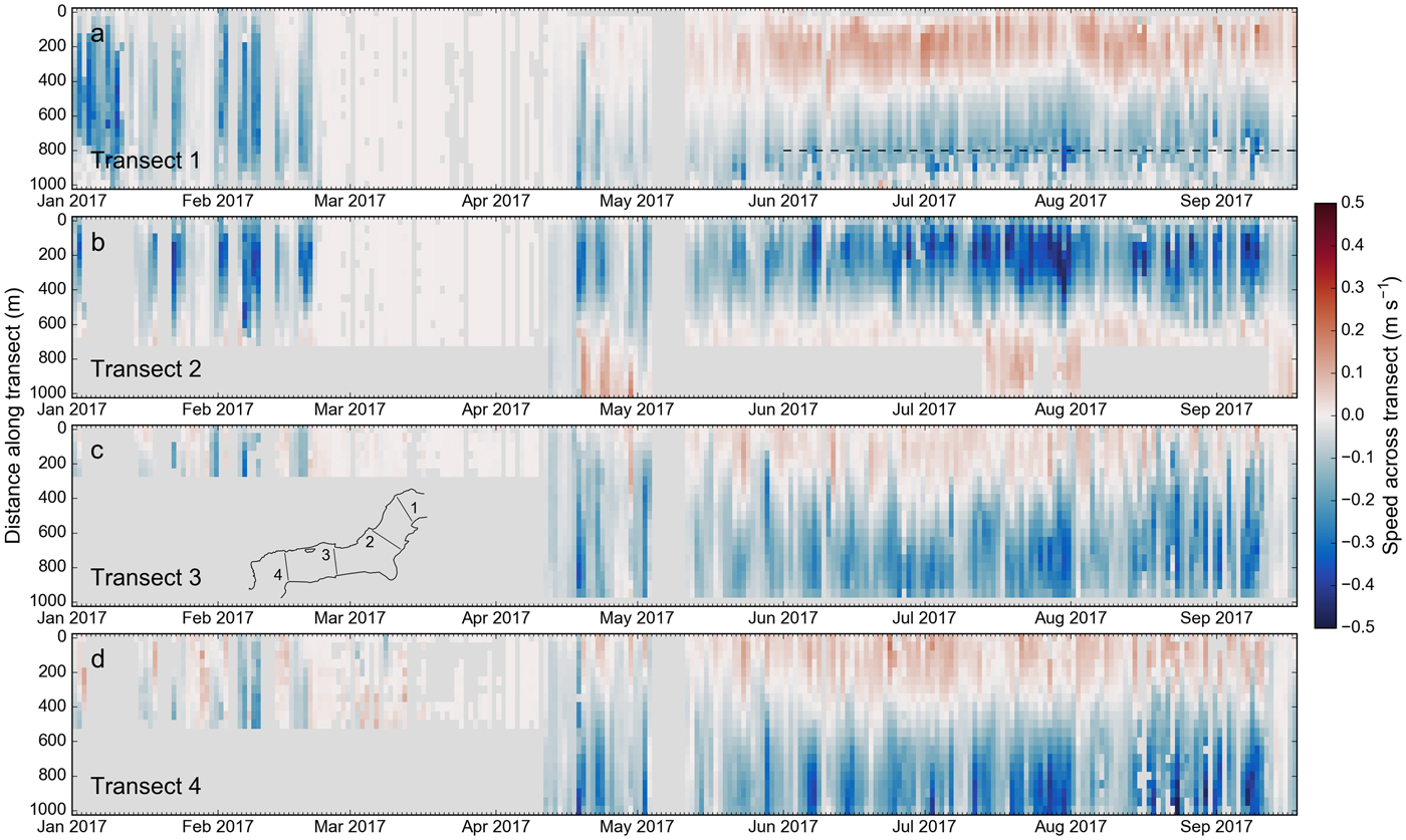
Figure 12, showing daily average flow across transects 1–4, provides a compact visualization of the flow patterns over the study period. Consistent color patterns during the summer indicate relatively persistent current patterns, likely controlled by ample glacier runoff. Highest flow speeds are typically found in mid to late summer (late July to September 2017), reaching and occasionally exceeding 0.5 m s−1 on a daily average. The circulation patterns are more variable during the winter season, possibly due to strong wind events and lower plume activity. Between 25 February and 12 April 2017, ice mélange covered the fjord, resulting in minimal iceberg displacement during that time.
(a–d) Time series of daily average speeds across transects 1–4. The inset map in (c) shows the fjord along with transect locations. Colors reflect the speed perpendicular to the transect, with blue tones (negative speeds) indicating downfjord motion. Light gray colors indicate no data (due to camera failure, snow cover or fog). The ordinate reflects distance along the transect, with 0 m distance corresponding to the north end of the transects. Speeds are calculated for bins 50 m wide. For better readability, we show data from 2017 only. In the case of transect 1, velocities between  $\scriptstyle \sim $800 m (dashed line in panel a) and 1000 m distance are not trustworthy because they cover the outflowing plume close to the glacier terminus, where the 0.5 min−1 time-lapse frame rate was too low to capture the high velocities.
Extending from these initial interpretations, we are currently analyzing the velocity data in tandem with other field data. This work seeks to identify the key factors driving fjord circulation by correlating the derived velocities with forcing such as tides, wind and glacier runoff. In addition, forthcoming hydrodynamic modeling efforts will use our velocity fields as constraints.
6. CONCLUSIONS
We developed a workflow to track icebergs in proglacial fjords, using oblique time-lapse imagery and the Lucas-Kanade optical flow algorithm. We applied the workflow to >400 000 time-lapse photos taken at LeConte Bay, Alaska, between spring 2016 and fall 2017. The derived velocity fields provide a spatially and temporally comprehensive picture of iceberg motion, which, given the prevalence of small icebergs in LeConte Bay, represents near-surface fjord circulation. This is confirmed by comparing image-derived velocities to in-situ ADCP data, which yields best agreements for depth levels above  $\scriptstyle \sim $12 m. While the 0.5 min−1 camera frame rates used for our 18 month survey were sufficiently high in many cases, the fastest icebergs/currents were missed, especially in areas close to the cameras. Tests with a range of camera frame rates suggest ideal rates of at least 1 min−1 for settings similar to LeConte Glacier. Such high frame rates are feasible with high capacity storage cards, especially since image spatial resolution (and thus size) is of secondary importance for the tracking algorithm.
Application of our workflow to other fjords will be successful if iceberg concentrations are sufficiently high. The icebergs' size distribution will affect the interpretation of the resulting velocity fields, and only in fjords with predominantly small icebergs will iceberg motion reflect near-surface currents reliably. In addition to the camera frame rates, camera placement will be crucial for best results. Too low of an elevation leads to unwanted (flat) viewing angles, while too high of an elevation causes problems with clouds and fog. Ideally, the region of interest should be covered by at least two cameras for redundancy, and to allow for advanced filtering of the derived trajectories. If possible, the cameras should be deployed at locations spaced several hundred meters apart. Cameras that are close together have similar fields of view and tend to be affected by the same problems (snow cover, glare, etc.), which hampers advanced filtering of the tracking results and camera intercomparisons in general. Additionally, we recommend the use of shutterless cameras (to reduce the risk of failure), fixed focal length lenses (to ensure focal length does not change when servicing the cameras) and accurate GPS timing (for comparing photos from multiple cameras, photos and satellite imagery, or photos and GPS tracks of objects visible in the photos). Precisely synchronized timing together with dedicated camera placement would also enable stereoscopic analysis of iceberg geometry.
Though useful currently, our code has room for improvement and further development. An initial focus should be on developing a scheme to filter out cloudy scenes (currently done manually) and advanced filtering of faulty trajectories (currently done with fixed thresholds). Advanced filtering should incorporate data from multiple cameras rather than treating the data from each camera separately, as is done currently. Implementing a more sophisticated camera model is another priority, especially with regard to the use of cameras with larger lens distortions. Finally, it would be useful to implement alternative tracking algorithms, for example, based on sparse implementation of image matching (e.g., Schwalbe and Maas, Reference Schwalbe and Maas2017) or SIFT-like techniques (e.g., Lowe, Reference Lowe2004; Rublee and others, Reference Rublee, Rabaud, Konolige and Bradski2011). Algorithm performance should then be assessed with regard to the iceberg tracking task, thereby focusing on algorithm robustness, accuracy and computational demand.
ACKNOWLEDGEMENTS
This work was funded by the U.S. National Science Foundation (OPP-1503910, OPP-1504288, OPP-1504521 and OPP-1504191). We thank Captains Scott Hursey (MV ‘Pelican’) and Dan Foley (MV ‘Steller’) for vessel support, and Wally O'Brocta (Temsco Helicopters) for helicopter support. We also acknowledge assistance in the field from Chris Carr, Morgan Michels and Avery Stewart.
SUPPLEMENTARY MATERIAL
The supplementary material for this article can be found at https://doi.org/10.1017/jog.2018.105.
The code for the tracking workflow is available at https://bitbucket.org/ckien/iceberg_tracking/.
APPENDIX A. CALCULATION OF THE ΔZ TIME SERIES AND CORRESPONDING UNCERTAINTIES
The elevation difference between camera and icebergs (Δz) is required to project trajectories from image to map coordinates. Δz is affected by both tides and iceberg height. Here, we account for tides but lack stereo imagery to account for iceberg height. Our Δz time series thus reflects the elevation difference between camera and water surface.
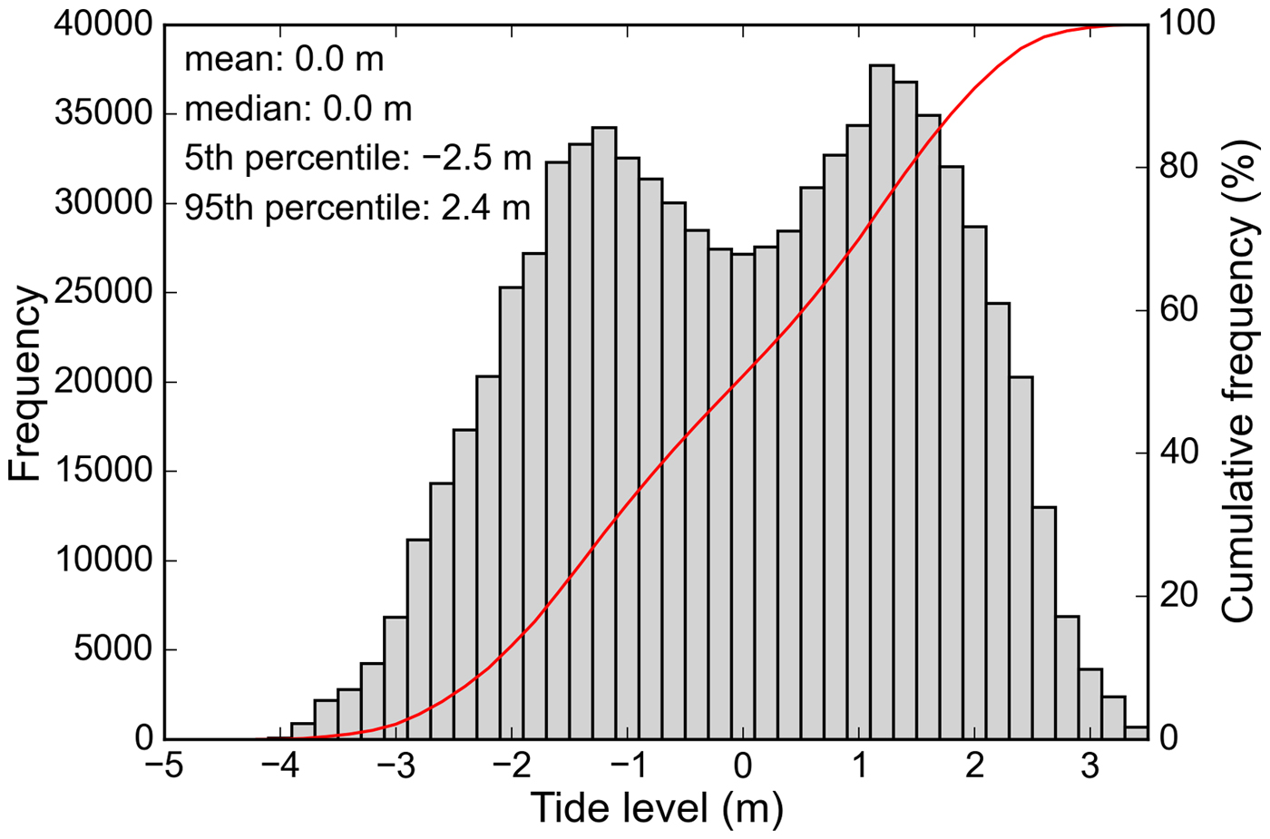
Our tide calculations are based on pressure measurements from moorings deployed in upper LeConte Bay. Between 1 April and 10 August 2016 (131 days), a SBE37 MicroCAT recorded pressure at  $\scriptstyle \sim $60 m depth. These pressure records were converted to depths and used as input for the Pytides tide model (https://github.com/sam-cox/pytides), which provided tide elevations at 1 minute intervals over the entire period of interest (March 2016–September 2017). The corresponding frequency distribution shows a bimodal distribution of tide levels with peaks at –1.2 and 1.2 m, and minimum/maximum tides at –3.8 and 3.6 m (Fig. 13). To check the quality of the tide prediction, we compared the modeled tides to tide measurements from a second mooring, deployed over 264 days from 15 August 2016–6 May 2017. The comparison of the two elevation time series yielded a normal distribution with a mean (μ) of 0.0 m and standard deviation (σ) of 0.21 m, confirming high quality of the tide prediction.
Frequency distribution of modeled tide levels during the period 20 March 2016–30 September 2017. The two peaks of the bimodal distribution are at –1.2 and 1.2 m, respectively. 90% of the tide elevations lie between –2.5 and 2.4 m. Reference surface is the mean tide level calculated over the study period.
Our camera elevations are known relative to the WGS84 ellipsoid, with a vertical uncertainty (1 σ) of 0.25 m (they were surveyed using a geodetic-quality Trimble NetRS GPS). To prevent biases in our Δz time series, tide elevations must be converted from orthometric to ellipsoidal heights. A geoid model could be considered for conversion, however, geoid models come with large uncertainties in the LeConte Bay area (e.g., 8.3 m (95% confidence interval) when using GEOID 12B (https://www.ngs.noaa.gov/GEOID/GEOID12B)). To avoid such uncertainties, we ran a Trimble NetRS GPS on our vessel while conducting multi-day surveys in LeConte Bay in May 2017. The difference between the GPS-derived water level (1 minute averages) and corresponding modeled tide elevations was –0.13 m (μ) and 0.11 m (σ). Subtracting 0.13 m from the modeled tide elevations resulted in the tide elevation time series relative to the WGS84 ellipsoid, which we then subtracted from the camera's elevation for the final Δz time series.
To estimate a combined uncertainty for the Δz time series, two uncertainties have to be considered in addition to the uncertainties introduced above. First, the vertical distance between GPS antenna and camera focal point is known with an uncertainty of approximately ±0.05 m, and thus adds a potential bias to the random uncertainty from the actual GPS processing (±0.25 m). The elevation difference between the boat's GPS antenna and the water is known with an uncertainty of ±0.1 m. This potential bias adds to the random uncertainty of ±0.11 m. Combining these uncertainties in a Monte Carlo fashion (10 000 runs) yields a normal error distribution, with μ = 0.0 m, σ = 0.35 m, and 5/95% percentiles of –0.58 and 0.58 m. These numbers suggest that the true Δz lies within ±58 cm of the modeled Δz (90% confidence). The corresponding positional error of a projected feature e p can be approximated as follows:
 $$ e_p = d \cdot \frac{\displaystyle{e_z}}{\Delta{}z - e_z}, $$
where d is the feature's horizontal distance from the camera, e z the error in elevation, and Δz the camera's elevation above water level. According to Eqn (A1), e p linearly increases with the feature's distance from the camera. With a Δz of 420 m and e z values of –0.58 and 0.58 m, this equation yields absolute positional errors between –1 and 1 m in the closest fjord portion (700 m horizontal distance from the cameras). The positional error lies between –7 and 7 m in the fjord portions farthest away from the cameras (at a horizontal distance of 5500 m). Given the linear relationship, e p corresponds to  $\scriptstyle \sim $0.14% of d for this particular e z–Δz combination. The same fraction quantifies the error in speed, which, lying between –0.14 and 0.14%, remains negligible.
Based on Eqn (A1), we can also assess projection and speed errors that result from neglecting iceberg heights. Assuming a large freeboard of 5 m (e z = 5), the positional error in the closest fjord portion (700 m horizontal distance) equals  $\scriptstyle \sim $8.5 m while reaching $\scriptstyle \sim $66.5 m at 5500 m horizontal distance from the cameras. In the case of e z = 5 m and Δz = 420 m, apparent speeds are $\scriptstyle \sim $1.2% faster than their true equivalents. Note that the fractional error in speed varies approximately linearly with e z (e.g, it is reduced to $\scriptstyle \sim $0.6% in the case of e z = 2.5 m and Δz = 420 m).


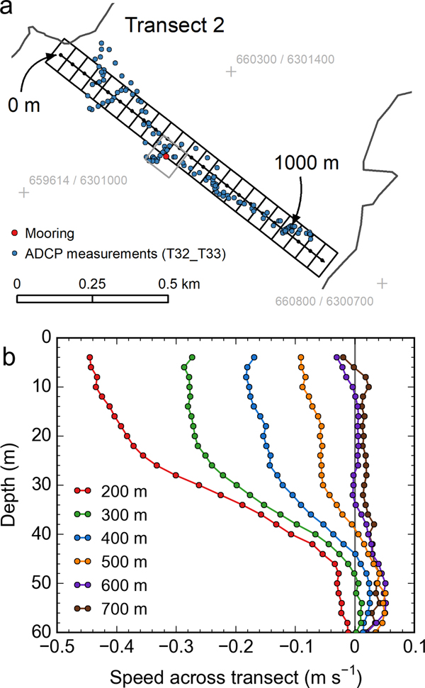


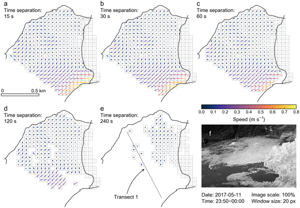

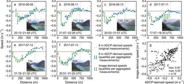


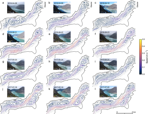

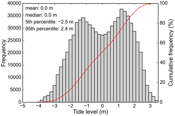


 Open access