


1. Introduction
Humanity has witnessed sovereign debt crises for hundreds of years. Foreign debt and default have been studied extensively in the literature, but recently the “forgotten history of domestic debt” has become an important research agenda started by Reinhart and Rogoff (Reference Reinhart and Rogoff2011a). Domestic debt is large and plays a significant role in the history of sovereign defaults. Worldwide, domestic debt has accounted for a large fraction of total public debt in the postwar era. This paper contributes to the literature by establishing new stylized facts about domestic and foreign debt and default and proposing a new theory that can rationalize them.
Using data on 89 emerging economies in the years 1950–2012 we establish two stylized facts: (i) governments issue debt on both domestic and foreign markets and the correlation between the two debts is low, (ii) defaults are mostly selective on either domestic or foreign debt.
We build a dynamic sovereign default model to explain these facts. In a standard sovereign default model, output fluctuates, a government borrows from foreign risk-neutral investors to smooth consumption of domestic households, and it defaults when the costs of repayment are greater than the costs of default (Aguiar and Gopinath, Reference Aguiar and Gopinath2006; Arellano, Reference Arellano2008; Eaton and Gersovitz, Reference Eaton and Gersovitz1981). We extend the standard model by allowing the government to also issue debt to domestic households and default selectively. The government has a rationale to issue debt on the domestic market because it wants to smooth tax distortions, which is a standard mechanism explaining domestic borrowing in the public finance literature (Barro, Reference Barro1979).
In the model domestic and foreign debts and selective defaults arise endogenously. The economy is subject to volatile output and a deadweight loss from taxation that can vary over time. Markets are incomplete, the government issues bonds to domestic and foreign investors, and it cannot commit to future repayments. The government has three means of financing: taxes and two defaultable bonds. Domestic bonds are bought by domestic households and foreign bonds are bought by risk-neutral foreign investors. From the government’s perspective, the two debts are distinguishable, because different investors hold them, and the government cares differently about their welfare. A government weighs the benefits of defaulting and holding on to borrowed resources against default costs, which consist of a temporary market exclusion and an output loss.
Domestic and foreign debts are hardly similar. Foreign debt issuance and repayment involve transferring resources into and out of an economy, which can help to achieve consumption smoothing over the business cycle. Domestic debt cannot achieve this, as its issuance and repayment occur within an economy: domestic borrowing does not bring in additional resources. In the absence of distortions, taxes and domestic debt are perfect substitutes. The tax wedge, however, breaks this Ricardian equivalence and distinguishes between tax-financed and debt-financed expenditures. The government chooses the optimal combination of two debts to smooth the two exogenous processes. In equilibrium, the government mostly relies on domestic debt to smooth the tax wedge and mostly relies on foreign debt to smooth the output shock.
Defaults on both markets are triggered by a negative output shock but occur subject to different histories of debt stock accumulations. Foreign default occurs when the accumulated stock of foreign debt is high, after a boom followed by a one-off sudden, deep recession. A government repays domestic debt with taxes only when the tax wedge is low. When the tax wedge is high, a government prefers to issue domestic debt rather than collect taxes. Domestic default occurs in a recession after a period of persistently high tax wedge.
We estimate output and tax wedge processes in the sample of emerging economies and default penalty parameters are calibrated to match the average frequencies of different types of defaults. The inclusion of domestic debt into the standard model brings the average level of the total public debt close to the data. Our model, with one-period bonds, delivers 37% total debt-to-GDP, close to the numbers observed empirically in emerging economies, and much higher than the standard sovereign default model with only foreign debt. The model successfully predicts the frequencies of selective defaults, the average debt-to-GDP ratios, as well as several untargeted moments including the low correlation between the two debts and average output paths around domestic and foreign default. It is able to explain several salient features of emerging markets business cycles such as the countercyclical spreads, excess consumption volatility, countercyclical trade balance, and procyclical fiscal policy.
A key insight of the paper is that in equilibrium, governments use domestic and foreign debt instruments for distinct purposes, driven by the nature of the shocks they face. Specifically, the government primarily relies on domestic debt to smooth tax distortions, and on foreign debt to smooth output fluctuations. This separation emerges naturally from our framework, where two orthogonal shocks, one affecting the tax wedge and another affecting output, create distinct incentives for default on domestic and foreign obligations. By isolating the two dimensions, the model captures the observed weak correlation between domestic and foreign defaults and replicates key empirical regularities across emerging economies.
Literature review. The canonical sovereign default model of Eaton and Gersovitz (Reference Eaton and Gersovitz1981) and its quantitative versions of Aguiar and Gopinath (Reference Aguiar and Gopinath2006) and Arellano (Reference Arellano2008) are built around the four main assumptions: single asset, risk-neutral foreign investor, one shock, and exogenous default penalties. The literature has since been tasked with relaxing each of those assumptions, as motivated by empirical regularities that the canonical model found hard to replicate. Our motivation is also empirical: quantitative importance of domestic debt and a pattern of selectivity in sovereign defaults. Thus, our contribution extends the standard model by enriching the asset structure and investors’ heterogeneity. In our framework, foreign investors are risk-neutral, but domestic investors are risk-averse in the spirit of Lizarazo (Reference Lizarazo2013), which improves the debt pricing kernel, by allowing for risk aversion on the foreign investors’ side.
In our model taxes are distortionary, which creates incentives for a government to borrow domestically. Thus, the model is closely related to Pouzo and Presno (Reference Pouzo and Presno2022) and where a government defaults to mitigate tax distortions, albeit in a closed economy setting. Other contributions that study defaultable domestic debt in a closed economy setting include: Bocola (Reference Bocola2016), Coimbra (Reference Coimbra2020) and D’Erasmo and Mendoza (Reference D’Erasmo and Mendoza2016). By introducing two debt instruments, our framework improves the model fit in terms of debt-to-GDP ratios.
While both domestic and foreign debt obligations are real in our model, a recent strand of literature introduces nominal domestic debt, which enables a different form of selective default specifically, default through inflation. Governments can effectively reduce the real value of their domestic obligations by allowing higher inflation, without triggering the formal legal or reputational consequences of outright default. This mechanism is especially relevant for emerging markets, where domestic-currency-denominated debt is increasingly used as a tool of macroeconomic management. Studies such as Engel and Park (Reference Engel and Park2022) and Phan (Reference Phan2017), Du et al. (Reference Du, Pflueger and Schreger2020) model sovereigns’ incentives to inflate away their nominal liabilities, and show how inflation can serve as a politically and institutionally feasible way to achieve partial default vis-à-vis domestic creditors while preserving external creditworthiness.
In our model, we assume that the process of tax collection is expensive and that this cost fluctuates over time. Two recent studies, Casalin et al. (Reference Casalin, Dia and Hallett2020) and Cerniglia et al. (Reference Cerniglia, Dia and Hallett2021) also investigate the stability of domestic public debt under a similar assumption. They explore the idea that governments face challenges when attempting to rapidly change tax policies. These studies demonstrate, albeit using a different framework, that ineffective tax collection can lead to the instability of public debt. Our model incorporates a similar mechanism, but we focus on examining the impact of external fluctuations in the tax base (TB) on both: sovereign default incentives and debt issuance policies.
Some recent contributions use alternative frameworks to study sovereign debt composition allowing for selective default. Erce and Mallucci (Reference Erce and Mallucci2018) study the impact of sovereign default on credit and trade in a two-bond economy, where domestic debt is held by domestic banks. Niepelt (Reference Niepelt2016) builds a theoretical model with overlapping generations and elections where a government weights default benefits to taxpayers against costs to creditors. Di Casola and Sichlimiris (Reference Casola and Sichlimiris2025) also use discrimination assumption to show how market segmentation can arise endogenously. Vasishtha (Reference Vasishtha2010) studies the selective nature of sovereign defaults but in equilibrium, contrary to empirical evidence, foreign default never happens. Several recent contributions study how debt composition affects default incentives under the assumption that a government cannot discriminate between domestic and foreign investors (Brutti, Reference Brutti2011; D’Erasmo and Mendoza, Reference D’Erasmo and Mendoza2021; Engler and Große Steffen, Reference Engler and Große Steffen2016; Gennaioli et al., Reference Gennaioli, Martin and Rossi2014; Guembel and Sussman, Reference Guembel and Sussman2009; Mengus, Reference Mengus2018; Sosa-Padilla, Reference Sosa-Padilla2018).Footnote 1
2. Stylized facts
The mechanism of foreign debt issuance and foreign default is well understood. The role that domestic debt plays—less so. Is domestic debt used by governments as a substitute for foreign debt, or are the two complementary? Are governments concerned about total debt issuance, or do they use two instruments to achieve different objectives? Do governments default on domestic debt and if so, do domestic and foreign defaults coincide? In this section, we shed light on these questions demonstrating empirical regularities.
Throughout the paper, we use the economic definition of domestic and foreign debt (residency of debt holder), as it creates clear differential incentives for a sovereign to default. However, the data on selective defaults and debt compositions usually come in legal definition (country’s legal framework applying to an issuance). The literature argues that the two definitions have been historically close to each other.Footnote 2
1. Governments issue debt on both domestic and foreign markets. The fact that governments use both domestic and foreign debt is a cross-country, systematic phenomenon confirmed in Figure 1. It plots domestic debt-to-GDP on the vertical axis against foreign debt-to-GDP on the horizontal axis after excluding default episodes. The vast majority of observations lie outside of the two axes.
Domestic vs foreign debt outstanding in emerging economies.Notes: Dots represent combinations of foreign and domestic sovereign debt outstanding in % of GDP after excluding crisis episodes. The dataset covers 70 developing economies (using World Bank classification) in the years 1950–2010. In total, 1686 observations are plotted in this figure. See the Online Appendix for details.Source: Own calculations based on Panizza (Reference Panizza2008) and Reinhart and Rogoff (Reference Reinhart and Rogoff2011b).

In our dataset, covering 70 emerging economies over the 1950–2010 period, we do not find any distinct and stable relationship between domestic and foreign debt. The correlation between domestic and foreign debt plotted in Figure 1 is 0.17. Table 1 provides more data on cross-country debt statistics. The average foreign debt-to-GDP is 31.2%, while the average domestic debt is 21.3%, meaning that in developing economies, about 40% of total sovereign debt is held domestically. We also calculate debt issuance-to-GDP numbers. Developing economies issue on average 0.84% of new foreign and 1.04% new domestic debt-to-GDP every year. The correlation between issuances is 0.27, which is slightly higher, but still low, both statistically and economically. This of course masks some variation over time and across countries; one can find examples of countries where there are periods of high domestic and foreign debt correlations, as well as other examples of countries where there are episodes of high negative correlation. This highlights a need for a theoretical exploration of domestic and foreign debt issuance that could identify the factors driving the correlation between the two.
Sovereign debt statistics

Notes: The table presents statistics for domestic and foreign sovereign debt in developing economies (i.e. after excluding advanced economies according to World Bank classification). The statistics are calculated after excluding crisis episodes. The total number of economies with available data on domestic debt is 74, foreign debt is 77, and on both is 70. The years are 1950–2010. Spread data is calculated as dollar returns for US-based investors on foreign and local currency bonds in 16 developing economies based on J.P. Morgan GBI-Broad local currency government bond and J.P. Morgan EMBI foreign currency government bond and is calculated as annualized monthly yields-to-maturity, the years are 2002–2017.Source: Own calculations based on Panizza (Reference Panizza2008) and Reinhart and Rogoff (Reference Reinhart and Rogoff2011b). Spread data from Borri and Shakhnov (Reference Borri and Shakhnov2017).
The composition of foreign and domestic debt is important. Empirically it has been shown that, among other things, it determines the size of fiscal multipliers (Priftis and Zimic, Reference Priftis and Zimic2021), and the size of international spillovers (Borri and Shakhnov, Reference Borri and Shakhnov2017).
Sovereign defaults statistics

Notes: The table presents debt default statistics for developing economies. The total number of countries in the dataset is 127, of which 89 are developing, the timeframe is 1950–2012, the frequency of observations is annual, and the total number of observations is 6259. A domestic default is defined as either a de jure domestic default crisis or an inflation crisis, which are defined in the source dataset. A total default is defined as a domestic and an external default starting in the same year. The number of defaulters is defined as the number of countries that experienced at least one episode of each type of default. The frequencies are calculated as the number of default episodes divided by the number of years. The mean frequencies and the mean lengths of each type of default are calculated among the respective defaulters only (mean and length of foreign default are calculated among foreign defaulters etc.).
Source: Own calculations based on Reinhart and Rogoff (Reference Reinhart and Rogoff2011b).
The average spread on domestic debt in the available data is 7.23% and is visibly higher than the spread on foreign debt 5.05% in developing economies. This may indicate that markets attach a higher probability of default on domestic debt than on foreign debt with comparable characteristics, either through outright de jure default or because of a risk of partial default via inflation.
2. Defaults are mostly selective. The data on defaults come from the updated database accompanying Reinhart and Rogoff (Reference Reinhart and Rogoff2011b) and cover up to 130 countries for the years 1800-2014. As the dates of the domestic and foreign debt crises sometimes overlap, there are many ways to calculate the final number of events. We focus on the postwar period. When a government, in a given year, defaulted de jure on both domestic and foreign debt we label this event as total default. There are only 18 such instances. When a government, in a given year, defaulted only on its foreign debt, we label it as foreign default. There are 166 such instances. Similarly, when a government, in a given year, defaulted only on its domestic debt, we label this event as domestic default.
We recognize that hyperinflation is a de facto way to default on domestic debt. Inflation crises help to reduce the burden of local currency-denominated debt. This debt was often issued domestically and sold to domestic residents. This is consistent with our theoretical framework, which is a real model of de facto defaults. There are 45 instances of de jure domestic defaults and 143 de fact domestic defaults via inflation crises. We define domestic default as either of the two and calculate 165 instances. The table shows that sovereign selective default is a systematic phenomenon that calls for a unified theory of domestic and foreign debt and selective defaults.Footnote 3
How can a government default on foreign investors while repaying domestic investors or vice versa? Among the tools that governments use to discriminate against types of bondholders, the most popular are capital controls, exchange controls and freezes on deposits. In 1990 Brazil defaulted on its domestic debt but kept servicing its foreign debt. All foreign exchange transactions were directed through the central bank. In 1998 Russia defaulted on both foreign and domestic debt, imposing capital and exchange rate controls. Russia kept servicing debts to foreign investors and domestic households, so it effectively defaulted only on domestic debt held by firms. Argentina’s 2001 default is often considered as a model calibration case of foreign default, although in fact, it was a total default. Firstly, all resident-held bonds, denominated in both domestic and foreign currency, were converted to government-guaranteed loans, which were all later converted to pesos at below-market exchange rate. Secondly, 60% of the debt defaulted on in December 2001 was held by Argentinians.Footnote 4
Our debt/default dataset includes 127 economies, of which we concentrate on 89 economies that are classified as developing.Footnote 5 Of those, all 89 experienced a foreign default at some point in the years 1950–2012. On the domestic market, 38 experienced a de jure domestic default and 42 experienced an inflation crisis; 64 economies domestic default (either of the two). Only 19 economies experienced a simultaneous total default.
We calculate the frequency of each default only for economies that experienced at least one default. Foreign defaults happen on average 2.99% of the time, while domestic defaults are more common, happening 4.09% of the time. Total defaults are rare, happening on average 1.58% of the time. Foreign defaults last on average 6.81 years, while domestic defaults are shorter lasting on average for 4.08 years.
In the next section we build a theory to explain why governments issue debt on domestic and foreign markets and why they tend to default selectively. The model is quantitative and will be calibrated to replicate these observed data regularities.
3. The model
Let time be indexed by $t=0,1,2,\ldots$
The economy has an exogenous stochastic stream of income
$t=0,1,2,\ldots$
The economy has an exogenous stochastic stream of income $y_t \in \mathbb{Y}$
, which is a Markov process. In each period
$y_t \in \mathbb{Y}$
, which is a Markov process. In each period $t$
the government covers a fixed exogenous stream of expenditures
$t$
the government covers a fixed exogenous stream of expenditures $g$
and decides either to repay or default on outstanding foreign and domestic debts. When the government chooses to default, the economy suffers from output penalties and is excluded from borrowing on the market where the default happened for a random number of periods. We allow the expected exclusion durations and output costs to differ between the two markets. When the government chooses to repay to either type of investor, it issues new bonds on the respective market.
$g$
and decides either to repay or default on outstanding foreign and domestic debts. When the government chooses to default, the economy suffers from output penalties and is excluded from borrowing on the market where the default happened for a random number of periods. We allow the expected exclusion durations and output costs to differ between the two markets. When the government chooses to repay to either type of investor, it issues new bonds on the respective market.
3.1 Households
Households are identical and risk-averse. Their instantaneous utility is given by the CRRA function over consumption:
 \begin{equation} u(c_t) =\frac {c_t^{1-\sigma }}{1-\sigma }. \end{equation}
Households save using domestically issued government bonds $b_d$
. They face a budget constraint, which is dependent on the government’s decision to default on their savings (
$b_d$
. They face a budget constraint, which is dependent on the government’s decision to default on their savings ( $\delta _d$
).Footnote
6
When the government repays both debts, households’ budget constraint reads:
$\delta _d$
).Footnote
6
When the government repays both debts, households’ budget constraint reads:
 \begin{equation} c^i=y^i-T(1+\tau )+(1-\delta _d)\left(b_d-q^i_d b_d'\right), \quad i \in \{r,fd,dd,td\} \end{equation}
where $b_d$
is the amount of domestic debt owed and repaid by the government to households,
$b_d$
is the amount of domestic debt owed and repaid by the government to households, $b_d'$
is the new issuance of government domestic debt,
$b_d'$
is the new issuance of government domestic debt, $q^i_d$
is the domestic bond’s discount price, which depends on the government default decisions. Output
$q^i_d$
is the domestic bond’s discount price, which depends on the government default decisions. Output $y^i$
and consumption
$y^i$
and consumption $c^i$
also depend on the government repayment/default decision.
$c^i$
also depend on the government repayment/default decision. $T$
is the amount of taxes raised by the government. Whenever taxes are negative, the household budget constraint is
$T$
is the amount of taxes raised by the government. Whenever taxes are negative, the household budget constraint is $c^r=y-T(1-\tau )+b_d-q_d^r b_d'$
, so that rebates or transfers are not distortionary.
$c^r=y-T(1-\tau )+b_d-q_d^r b_d'$
, so that rebates or transfers are not distortionary. $\tau$
is an exogenous deadweight loss from taxation that drives a wedge between the benefit of taxation for the government and the cost of taxation for the agents. Here, we follow an idea from Chari et al. (Reference Chari, Kehoe and McGrattan2007), that many models are equivalent to a prototype model with time-varying wedges. In this case, many models with endogenous tax distortions can be mapped into our prototype specification with an exogenous tax wedge that resembles a time-varying labor tax wedge.Footnote
7
$\tau$
is an exogenous deadweight loss from taxation that drives a wedge between the benefit of taxation for the government and the cost of taxation for the agents. Here, we follow an idea from Chari et al. (Reference Chari, Kehoe and McGrattan2007), that many models are equivalent to a prototype model with time-varying wedges. In this case, many models with endogenous tax distortions can be mapped into our prototype specification with an exogenous tax wedge that resembles a time-varying labor tax wedge.Footnote
7
Output in this economy is an exogenous endowment that evolves according to an $AR(1)$
stochastic process in logs:
$AR(1)$
stochastic process in logs:
 \begin{equation} log(y_{t})=\rho _y log(y_{t-1})+u_t \qquad u_t \sim \mathcal{N}\big(0, \epsilon ^2_y\big). \end{equation}
The penalties that the government faces because of default are twofold. The government is excluded from the market and faces probabilities of returning to borrowing: $\theta _f$
to foreign and
$\theta _f$
to foreign and $\theta _d$
to the domestic market. In the default periods, the government also suffers an output cost, that is assumed to be asymmetric as in Arellano (Reference Arellano2008):
$\theta _d$
to the domestic market. In the default periods, the government also suffers an output cost, that is assumed to be asymmetric as in Arellano (Reference Arellano2008):
 \begin{equation} y^{i}_{t}=\min \{y_t, \gamma _i y\} \qquad i=\{\, fd,dd,td\}, \end{equation}
where $y^{i}$
is output in either domestic or foreign or total default,
$y^{i}$
is output in either domestic or foreign or total default, $y$
is the mean of the output process and
$y$
is the mean of the output process and $\gamma _i$
takes the separate values for domestic and foreign default and the multiple of two for total default. The cost function assumes the asymmetric default costs so that the default is more costly with high output realizations.
$\gamma _i$
takes the separate values for domestic and foreign default and the multiple of two for total default. The cost function assumes the asymmetric default costs so that the default is more costly with high output realizations.
Similarly to output, the tax wedge evolves according to an $AR(1)$
in logs around the mean
$AR(1)$
in logs around the mean $\bar {\tau }$
:
$\bar {\tau }$
:
 \begin{align} &\tau _t=\bar {\tau } \tilde {\tau }_t \end{align}
 \begin{align} &log(\tilde {\tau }_t)=\rho _{\tau }log(\tilde {\tau }_{t-1})+v_t \qquad v_t \sim \mathcal{N}\big(0, \epsilon ^2_{\tau }\big). \end{align}
3.2 Recursive equilibrium
We define a recursive equilibrium in which domestic households, foreign investors and the government act sequentially and the government acts with discretion. The aggregate state of the economy is given by two endogenous debts $(b_d,b_f)$
and two exogenous processes for income and the tax wedge
$(b_d,b_f)$
and two exogenous processes for income and the tax wedge $s=(y,\tau )$
. Every period, the government decides whether to repay its two outstanding debts, default on domestic debt, default on foreign debt or default on both:
$s=(y,\tau )$
. Every period, the government decides whether to repay its two outstanding debts, default on domestic debt, default on foreign debt or default on both:
 \begin{equation} V^0 \left(b_d,b_f,s\right)=max \big\{V^r \left(b_d,b_f,s\right),V^{dd} \left(b_f,s\right),V^{fd} \left(b_d,s\right),V^{td}(s)\big\} \end{equation}
The government’s default decisions are summarized by default indicators $\delta ^i_j$
assuming value 1 in the case of default, where subscript
$\delta ^i_j$
assuming value 1 in the case of default, where subscript $j$
stands for the defaulted debt: foreign and domestic (
$j$
stands for the defaulted debt: foreign and domestic ( $j=f,d$
) and superscript
$j=f,d$
) and superscript $i$
stands for the current state: repayment, foreign default and domestic default (
$i$
stands for the current state: repayment, foreign default and domestic default ( $i=r,fd,dd$
). It is sufficient to define two default indicators for repayment periods:
$i=r,fd,dd$
). It is sufficient to define two default indicators for repayment periods: $\delta ^r_{f}, \delta ^r_{d}$
(repayment decision is taken with both equal to zero and total default decision is taken with both equal to one) and one for each of the two selective default periods:
$\delta ^r_{f}, \delta ^r_{d}$
(repayment decision is taken with both equal to zero and total default decision is taken with both equal to one) and one for each of the two selective default periods: $\delta ^{fd}_{d}, \delta ^{dd}_{f}$
. The government’s choices are presented graphically in Figure 2, where tree branches correspond from the left to the right to repayment, total, selective foreign and selective domestic defaults.
$\delta ^{fd}_{d}, \delta ^{dd}_{f}$
. The government’s choices are presented graphically in Figure 2, where tree branches correspond from the left to the right to repayment, total, selective foreign and selective domestic defaults.
Government decision tree.Notes: When both markets are open ( $V^0$
), the government can decide to repay both debts (
$V^0$
), the government can decide to repay both debts ( $V^r$
), default on both debts (
$V^r$
), default on both debts ( $V^{td}$
), repay only domestic debt (
$V^{td}$
), repay only domestic debt ( $V^{fd}$
) or repay only foreign debt (
$V^{fd}$
) or repay only foreign debt ( $V^{dd}$
). Subsequent possible choices are depicted on the lower branches of the decision tree.
$V^{dd}$
). Subsequent possible choices are depicted on the lower branches of the decision tree.

If the government decides to repay it solves the following problem:
 \begin{equation} V^r\left(b_d,b_f,s\right)=\underset {b_d',b_f'}{max} \Big \{ u(c^r) + \beta {\mathbb E}_{} \left [ V^0(b_d',b_f',s' \right ] \Big \} \end{equation}
subject to four constraints: the households’ budget constraint (2), the foreign bond price schedule, the domestic bond price schedule and the government budget constraint. The foreign bond price schedule is given by:
 \begin{equation} q^r_f \left(b'_d,b'_f,s\right)=\frac { {\mathbb E}_{} \left [ 1-\delta ^r_{f} \left(b'_d,b'_f,s' \right) \right ]}{1+r} \end{equation}
where $q^r_f$
is the discount price of a government bond issued with foreign investors
$q^r_f$
is the discount price of a government bond issued with foreign investors $b'_f$
, who are risk-neutral, deep-pocket and have access to international risk-free rate
$b'_f$
, who are risk-neutral, deep-pocket and have access to international risk-free rate $r$
, and
$r$
, and $\delta ^r_{f}$
is the indicator of the government’s decision to default on foreign debt. A risk-free foreign investor assumption is employed by the vast majority of the literature. Unlike foreign, we assume that domestic investors are risk-averse.Footnote
8
The risk-averse price of domestic debt is dynamic and depends on six states: two exogenous shocks, two debts issued and two debts outstanding (as they all affect the marginal utility of consumption). Unlike in models facing risk-neutral marginal investors, the fluctuations in both current consumption and expected consumption affect debt discount prices. The domestic bond price schedule reads:
$\delta ^r_{f}$
is the indicator of the government’s decision to default on foreign debt. A risk-free foreign investor assumption is employed by the vast majority of the literature. Unlike foreign, we assume that domestic investors are risk-averse.Footnote
8
The risk-averse price of domestic debt is dynamic and depends on six states: two exogenous shocks, two debts issued and two debts outstanding (as they all affect the marginal utility of consumption). Unlike in models facing risk-neutral marginal investors, the fluctuations in both current consumption and expected consumption affect debt discount prices. The domestic bond price schedule reads:
 \begin{align} &q^r_d \left(b_d,b_f,b'_d,b'_f,s\right)=\notag \\ &=\beta \frac {{\mathbb E}_{} \left [ \left(1-{\delta ^r_{f}}'\right) \big(1-{\delta ^r_{d}}'\big) u_c\big ({c^r}'\big ) +{\delta ^r_{f}}'(1-{\delta ^r_d}') u_c\big ({c^{fd}}'\big ) \right ] } {u_c\left (c^r\right )}, \end{align}
where future expected utility consists of two parts: one related to repayment ( $\delta ^r_{f}=\delta ^r_{d}=0$
) and one to foreign default (
$\delta ^r_{f}=\delta ^r_{d}=0$
) and one to foreign default ( $\delta ^r_{f}=1$
). Only then is domestic debt serviced so it is a valid savings vehicle that enables intertemporal consumption smoothing. In (10) state space notation for default indicators and consumption levels has been suppressed to facilitate legibility. The last constraint is the government budget constraint:
$\delta ^r_{f}=1$
). Only then is domestic debt serviced so it is a valid savings vehicle that enables intertemporal consumption smoothing. In (10) state space notation for default indicators and consumption levels has been suppressed to facilitate legibility. The last constraint is the government budget constraint:
 \begin{equation} T+q^r_db'_d +q^r_f b'_f=g+b_d+b_f. \end{equation}
Second, if the government defaults on foreign debt (but services its domestic obligations) the economy suffers an output cost, with the probability $1-\theta _f$
is excluded from the foreign debt market (and remains only on domestic one) and the government can still decide to also default on domestic debt (yielding total default). The government’s problem is:
$1-\theta _f$
is excluded from the foreign debt market (and remains only on domestic one) and the government can still decide to also default on domestic debt (yielding total default). The government’s problem is:
 \begin{equation} V^{fd}(b_d,s)=\underset {b_d'}{max} \Bigg \{ u(c^{fd}) + \beta {\mathbb E}_{} \left [ \theta _f V^0 \left(0,b_d',s'\right) +(1-\theta _f) max\big \{V^{fd}\left(b_d',s'\right),V^{td}(s')\big \} \right ] \Bigg \} \end{equation}
subject to households’ budget constraint (2), households’ first-order condition
 \begin{equation} q_d^{\, fd}\big(b_d,b'_d,s\big)=\beta \frac {{\mathbb E}_{} \left [ \theta _f \left (1-{{\delta _{d}^{r}}'}\left (.,0,.\right )\right ) u_c\left ({c^r}'\left (.,0,. \right ) \right ) +\left (1-\theta _f\right ) \left (1-{\delta _{d}^{fd}}'\right )u_c\left ({c^{fd}}'\right ) \right ] } {u_c\left (c^{fd}\right )}, \end{equation}
where expected future marginal utility consists of two parts: one related to readmission to foreign markets and one related to foreign default, where $\delta ^{fd}_{d}$
is the probability of government going from foreign into total default. In (13) some arguments have been suppressed to facilitate legibility. The last is the government budget constraint:
$\delta ^{fd}_{d}$
is the probability of government going from foreign into total default. In (13) some arguments have been suppressed to facilitate legibility. The last is the government budget constraint:
 \begin{equation} T+q^{\, fd}_d b'_d =g+b_d. \end{equation}
Third, if the government decides to default selectively on domestic debt it remains active on the foreign market, comes back to domestic borrowing with the probability $\theta _d$
, suffers the domestic output penalty and can still default on foreign debt:
$\theta _d$
, suffers the domestic output penalty and can still default on foreign debt:
 \begin{equation} V^{dd} \left(b_f,s\right)=\underset {b_f'}{max} \Bigg \{ u(c^{dd}) + \beta {\mathbb E}_{} \left [ \theta _d V^0\left(b'_f,0,s'\right) +(1-\theta _d) max\big \{V^{dd}\left(b_f',s'\right),V^{td}(s')\big \} \right ] \Bigg \} \end{equation}
subject to households’ budget constraint (2), the foreign bond price schedule
 \begin{equation} q^{dd}_f\left(b'_f,s\right)= \theta _d \frac { {\mathbb E}_{} \left [ 1-{\delta _{f}^{r}}\left(b'_f,0,s'\right) \right ] } {1+r}+(1-\theta _d)\frac { {\mathbb E}_{} \left [ 1-{\delta _{f}^{dd}}\left(b'_f,s'\right) \right ] } {1+r}, \end{equation}
which is a probabilities-weighted sum of the price of foreign debt in repayment and foreign debt in domestic default, with $\delta _{d}^{fd}$
being the probability of the government going from foreign default into total default. The last is the government budget constraint:
$\delta _{d}^{fd}$
being the probability of the government going from foreign default into total default. The last is the government budget constraint:
 \begin{equation} T+q^{dd}_fb'_f =g+b_f. \end{equation}
Fourth, if the government decides to pursue total default, the economy suffers the output penalties for both domestic and foreign default, and the government comes back to the international and domestic markets with probabilities $\theta _f$
and
$\theta _f$
and $\theta _d$
respectively. The government’s problem is summarized by:
$\theta _d$
respectively. The government’s problem is summarized by:
 \begin{align} V^{td}(s)=u(c^{td})&+\beta {\mathbb E}_{} \left [ \theta _f\theta _d V^0(0,0,s) + \theta _f(1-\theta _d)V^{dd}(0,s')\right.\nonumber\\ &\left.+ (1-\theta _f)\theta _dV^{fd}(0,s')+(1-\theta _f)(1-\theta _d)V^{td}(s') \right ] \end{align}
subject to households’ budget constraint (2) and the government budget constraint
 \begin{equation} T=g. \end{equation}
Let $B=\{b_d,b_f\}$
define endogenous and
$B=\{b_d,b_f\}$
define endogenous and $s=\{y,\tau \}$
define exogenous states in the economy.
$s=\{y,\tau \}$
define exogenous states in the economy.
Finally, the default schedules are derived from the government’s choice of value functions associated with repayment and defaults:
 \begin{align} &\text{Repayment: } &\delta ^r_f=0, \delta ^r_d=0 & \iff V^r \geq max\big \{ V^{fd}, V^{dd}, V^{td}\big \} \nonumber\\[-12pt]\end{align}
 \begin{align} &\text{Foreign default: }& \delta ^r_f=1, \delta ^r_d=0 & \iff V^{fd} \gt max\big \{ V^{r}, V^{dd}, V^{td} \big \} \nonumber\\[-12pt]\end{align}
 \begin{align} &\text{Domestic default: } & \delta ^r_f=0, \delta ^r_d=1 & \iff V^{dd} \gt max\big \{ V^{r}, V^{fd}, V^{td} \big \} \nonumber\\[-12pt]\end{align}
 \begin{align} &\text{Total default: } &\delta ^r_f=1, \delta ^r_d=1 & \iff V^{td} \gt max \big \{V^r, V^{fd}, V^{dd} \big \} \nonumber\\[-12pt]\end{align}
 \begin{align} &\text{Domestic repayment after FD:} &\delta ^{fd}_d=0 & \iff V^{fd} \geq V^{td} \nonumber\\[-12pt]\end{align}
 \begin{align} &\text{Domestic default after FD: }& \delta ^{fd}_d=1 & \iff V^{fd} \lt V^{td} \nonumber\\[-12pt]\end{align}
 \begin{align} &\text{Foreign default after DD: } & \delta ^{dd}_f=0 & \iff V^{dd} \geq V^{td} \nonumber\\[-12pt]\end{align}
 \begin{align} &\text{Foreign repayment after DD: } & \delta ^{dd}_f=1 & \iff V^{dd}\lt V^{td} \end{align}
Definition 1.
The recursive competitive equilibrium is defined as four sets of default schedules $\{\delta ^r_d(B,s),\delta ^r_f(B,s),\delta ^{fd}_d(b_d,s),\delta ^{dd}_f(b_f,s)\}$
, four sets of debt discount prices
$\{\delta ^r_d(B,s),\delta ^r_f(B,s),\delta ^{fd}_d(b_d,s),\delta ^{dd}_f(b_f,s)\}$
, four sets of debt discount prices $\{q_f^r(B',s),q_d^r(B,B',s),$ $q_f^{dd}(b_f,s),q_d^{fd}(b_d,b'_d,s)\}$
, four sets of government debt issuance policies
$q_f^{dd}(b_f,s),q_d^{fd}(b_d,b'_d,s)\}$
, four sets of government debt issuance policies $\{b'_f(B,s), b'_d(B,s), {b'}_f^{dd}(b_f,s),$ $ {b'}_d^{fd}(b_d,s)\}$
and four sets of consumptions
$ {b'}_d^{fd}(b_d,s)\}$
and four sets of consumptions $\{c^r,c^{dd},c^{fd},c^{td}\}$
conditional of exogenous processes
$\{c^r,c^{dd},c^{fd},c^{td}\}$
conditional of exogenous processes $\{y,\tau \}$
such that:
$\{y,\tau \}$
such that:
-
1) Taking prices $\{q_f^r,q_d^r, q_f^{dd},q_d^{fd}\}$
and government debt issuances
$\{b'_f, b'_d, {b'}_f^{dd}, {b'}_d^{fd}\}$
as given, households’ consumptions
$\{c^r,c^{dd},c^{fd},c^{td}\}$
satisfy the households’ budget constraints.
$\{q_f^r,q_d^r, q_f^{dd},q_d^{fd}\}$
and government debt issuances
$\{b'_f, b'_d, {b'}_f^{dd}, {b'}_d^{fd}\}$
as given, households’ consumptions
$\{c^r,c^{dd},c^{fd},c^{td}\}$
satisfy the households’ budget constraints.
-
2) Taking prices
$\{q^r_d, q^r_f, q_d^{\, fd}, q_f^{dd}\}$
as given, government’s default schedules
$\{\delta ^r_{f}, \delta ^r_{d}, \delta _{d}^{fd}, \delta _{f}^{dd}\}$
and debt issuance policies
$\{b'_d, b'_f, {b'}_f^{dd}, {b'}_d^{fd}\}$
solve the government’s optimization problems.
-
3) Given foreign default schedules
$\{\delta ^r_{f}, \delta _{f}^{dd}\}$
foreign debt prices
$\{q^r_f,q^{dd}_f\}$
satisfy foreign investors expected zero profits.
-
4) Given domestic default schedules
$\{ \delta ^r_{f}, \delta _{f}^{dd}\}$
, households’ consumptions
$\{c^r, c^{fd}\}$
and future expected default schedules, debt issuances and households’ consumptions, domestic debt prices
$\{q^r_d,q^{\, fd}_d\}$
satisfy households first-order conditions.


4. Numerical analysis
4.1 Calibration
To solve the model numerically, we assume functional forms for the exogenous processes and assign parameter values. The data availability dictates the choice of a frequency for the model. As default frequencies and debt-to-GDP ratios, are best thought of at annual frequency we set up the model annually. There are two sets of parameters in the model. The first set, presented in Table 2, consists of values that are standard in the literature or that can be directly calculated from the data. The second set, presented in Table 3, consists of values calibrated so that the model replicates a selection of statistics presented in Stylized Facts. We set the risk aversion coefficient $\sigma$
equal to 2 and the risk-free interest rate
$\sigma$
equal to 2 and the risk-free interest rate $r$
to
$r$
to $1.7\%$
yearly, which are the standard values in the literature. The discount factor
$1.7\%$
yearly, which are the standard values in the literature. The discount factor $\beta$
we set to 0.825, which is a yearly equivalent of the quarterly
$\beta$
we set to 0.825, which is a yearly equivalent of the quarterly $\beta =0.953$
found in Arellano (Reference Arellano2008).
$\beta =0.953$
found in Arellano (Reference Arellano2008).
We calculate the level of government expenditure as spending on public consumption (government purchases of goods and services). We use a new dataset by Michaud and Rothert (Reference Michaud and Rothert2018) who calculate government expenditure for a sample of advanced and emerging economies with a detailed breakdown into different spending categories. The average spending on public consumption-to-GDP in emerging economies is 3.8%.
Set parameters

We calculate persistence and standard deviation of output using our dataset introduced in Stylized Facts. Using the yearly output data series for the sample of 101 emerging economies, and de-trending using the HP filter, the mean of the estimates for $\rho _y$
is 0.69 and for
$\rho _y$
is 0.69 and for $\epsilon _y$
is 0.094.
$\epsilon _y$
is 0.094.
As there is no readily available measure of the tax wedge in the data, we identify the movements in the tax wedge via the movements in the TB. The two are inversely related.Footnote 9
Using the yearly data for the value-added taxes in 55 emerging economies (Prichard et al., Reference Prichard, Cobham and Goodall2014; World Tax Database, 2015) the estimate of $\rho _{\tau }$
is 0.71 and of
$\rho _{\tau }$
is 0.71 and of $\epsilon _{\tau }$
is 0.11. For the mean tax wedge
$\epsilon _{\tau }$
is 0.11. For the mean tax wedge $\bar {\tau }$
we take a conservative stand and parametrize it at 0.025, which is the lowest estimate of the static deadweight loss from taxation that we have found in the literature (Harberger, Reference Harberger1964). We assume that the two processes are uncorrelated. This will allow the model to isolate the endogenous spillover effects from the exogenous interdependence and is consistent with the data (empirically, the correlation is equal to 0.0095).Footnote
10
Finally, we set the values of the exclusion probabilities
$\bar {\tau }$
we take a conservative stand and parametrize it at 0.025, which is the lowest estimate of the static deadweight loss from taxation that we have found in the literature (Harberger, Reference Harberger1964). We assume that the two processes are uncorrelated. This will allow the model to isolate the endogenous spillover effects from the exogenous interdependence and is consistent with the data (empirically, the correlation is equal to 0.0095).Footnote
10
Finally, we set the values of the exclusion probabilities $\theta _d, \theta _f$
to match the lengths of foreign and domestic defaults evidenced in Table 4, resulting in
$\theta _d, \theta _f$
to match the lengths of foreign and domestic defaults evidenced in Table 4, resulting in $\gamma _f=0.147$
and
$\gamma _f=0.147$
and $\gamma _d=0.244$
. These are well within the range of parameters typically used in the literature.
$\gamma _d=0.244$
. These are well within the range of parameters typically used in the literature.
Calibrated parameters

Table 4 contains the values for the output penalties upon default $\gamma _d, \gamma _f$
, which we calibrate to match domestic and foreign default frequencies also evidenced in Table 4 of 3% on foreign, and 4.1% on domestic debt. This yields calibrated parameters of
$\gamma _d, \gamma _f$
, which we calibrate to match domestic and foreign default frequencies also evidenced in Table 4 of 3% on foreign, and 4.1% on domestic debt. This yields calibrated parameters of $\gamma _f=0.808$
and
$\gamma _f=0.808$
and $\gamma _d=1.0175$
. In the next subsections, we study the quantitative properties of the model, but the calibration exercise already indicates that to match the quantitative behavior of foreign debt and default, the model requires a significant output penalty upon default: output drops to 0.808 whenever it would be above this level during a default episode. Conversely, on the domestic market, the exclusion from borrowing is a sufficient threat and almost no additional output penalties are required to sustain domestic debt and match the domestic default frequency. Output drops to 1.0175 (slightly above the average) whenever it would be above that level during a default episode. This means that additional production penalties on the domestic market are only operational when the government intends to default with a high output.Footnote
11
$\gamma _d=1.0175$
. In the next subsections, we study the quantitative properties of the model, but the calibration exercise already indicates that to match the quantitative behavior of foreign debt and default, the model requires a significant output penalty upon default: output drops to 0.808 whenever it would be above this level during a default episode. Conversely, on the domestic market, the exclusion from borrowing is a sufficient threat and almost no additional output penalties are required to sustain domestic debt and match the domestic default frequency. Output drops to 1.0175 (slightly above the average) whenever it would be above that level during a default episode. This means that additional production penalties on the domestic market are only operational when the government intends to default with a high output.Footnote
11
We solve the model by discretizing the state space for income shocks and tax distortions using a variant of the Tauchen method to approximate a two-dimensional Markov process. Foreign and domestic bond asset positions are discretized using grids with 31 and 33 points, respectively. Income and tax distortion shocks are discretized using grids with 23 and 25 points, respectively. Value functions for repayment and selective defaults are computed iteratively through value function iterations combined with bond price updating, accounting for endogenous default decisions. We solve for equilibrium bond prices ensuring consistency with borrowers’ default incentives and lenders’ pricing through the Euler equation. The equilibrium policies and prices are obtained once the value and price functions converge within a prescribed tolerance. More details on the solution method, including grid construction, numerical acceleration techniques, and convergence criteria, are provided in the Online Appendix.
4.2 Policy functions
In this section we analyze default and debt issuance policies in the calibrated model. Throughout the analysis we find that the policies for foreign debt and default respond strongly to the changes in output and little (or not at all) to changes in the tax wedge. However, policies for domestic debt and default respond strongly to both output and the tax wedge. Even though markets are segmented, we also document spillovers from one market to the other.
Default sets. Figure 3 plots the default-repayment policies for foreign debt, and Figure 4 plots the default-repayment policies for domestic debt. The level of debt is plotted horizontally on each graph and the output (left panel) and the tax wedge (right panel) are plotted vertically.
Foreign default becomes more likely as the level of foreign debt goes up and as the output goes down. For high levels of output, any level of foreign debt is safe. There is almost no variability in the foreign default decision with respect to the tax wedge. The foreign default set is decreasing in output, therefore, the foreign interest rate is decreasing in output as well. Foreign default happens when the output suddenly drops.
Default sets for foreign debt in output (left) and tax wedge (right).Notes: The figure plots default sets on the foreign debt in the foreign assets-income space (left) and foreign assets-tax wedge space (right). The domestic debt level in both panels is set at 0, tax distortions, in the left panel, are set at 0.024, and income, in the right panel, is set at 0.86.

Default sets for domestic debt in output (left) and tax wedge (right).Notes: The figure plots default sets on the foreign debt in the foreign assets-income space (left) and foreign assets-tax wedge space (right). The foreign debt level in both panels is set at 0, tax distortions, in the left panel, are set at 0.024, and income, in the right panel, is set at 0.86.

Default on each debt becomes more likely when the output drops. Empirical work provides strong evidence that domestic and foreign defaults are associated with substantial and prolonged contractions in output (Reinhart and Rogoff, Reference Reinhart and Rogoff2011a; Schmitt-Grohé and Uribe, Reference Schmitt-Grohé and Uribe2017). Domestic default is not only driven by tax wedge, but (due to the specification of the default costs), it also depends on output fluctuations. Domestic default becomes more likely as the tax wedge increases. Domestic default happens only with low output. The medium and high output levels render the domestic debt virtually safe.
Debt issuance. Figure 5 plots the bond issuance policies, i.e. future assets as a function of today’s assets, in the left panel for foreign assets and in the right panel for domestic assets. Lines represent different output levels. In the Figure we also plot the 45-degree line, to show when the economy issues more debt (below) and less debt (above) than is currently outstanding. The economy accumulates foreign debt when output is high due to the countercyclicality of the interest rate. An economy with a default risk engages in procyclical foreign borrowing, it increases its debt position when the output is high, and reduces its debt position when the output is low. Similar results for foreign debt are found across quantitative models of sovereign default. For the low output, there is a well-defined debt limit, below which the currently outstanding debt will be defaulted. As such, the new debt issuance drops to zero, as the economy optimally chooses to default. For the high output, there is also a maximum level of debt sustainable in equilibrium: at some point, the issuance policy crosses the 45-degree line, which means that it is optimal for the economy to reduce its foreign debt position. Foreign debt issuance is almost exclusively driven by output fluctuations. Foreign default occurs in a recession when foreign debt is high.
Foreign (left) and domestic (right) debt issuance policies as functions of output.Notes: The figure plots future assets position, as functions of outstanding assets position on the foreign market (left panel) and domestic market (right panel), for low output (red line) and high output (blue line). The 45-degree line is included in both panels to indicate when the future asset position is equal to the current asset position. The level of domestic assets in the left panel is set to 0, and the level of foreign assets in the right panel is set to 0. The level of the tax wedge in both panels is set to 0.024. Low output ( $y_L$
) is set to 0.86, and high output (
$y_L$
) is set to 0.86, and high output ( $y_H$
) is set to 1.12, in both panels.
$y_H$
) is set to 1.12, in both panels.

Domestic debt issuance is qualitatively different from foreign debt issuance. The assumed level of tax distortions is at the average. Irrespective of the output level, the government has incentives to save—both optimal issuance lines are above the 45-degree line. This suggests that tax distortions, and not output, are instrumental for debt build-up on domestic market, as we show in Figure 6. Interestingly, when domestic debt is low, and so it is safe, the incentives to save are stronger with higher output.
Foreign (left) and domestic (right) debt issuance policies as functions of tax wedge.Notes: The figure plots future assets position, as functions of outstanding assets position on the foreign market (left panel) and domestic market (right panel), for a low-tax wedge (red line) and high-tax wedge (blue line). The 45-degree line is included in both panels to indicate when the future asset position is equal to the current asset position. The low-tax wedge ( $\tau _L$
) is set to 0.018, and the high-tax wedge (
$\tau _L$
) is set to 0.018, and the high-tax wedge ( $y_H$
) is set to 0.035, in both panels. The level of output is set to 0.86, in both panels. The level of the asset outstanding on the other market is set to -0.18.
$y_H$
) is set to 0.035, in both panels. The level of output is set to 0.86, in both panels. The level of the asset outstanding on the other market is set to -0.18.

Conversely, in Figure 6 lines represent different levels of the tax wedge. The foreign debt policy is almost entirely driven by fluctuations in output and does not respond to changes in the tax wedge. Domestic debt strongly responds to the fluctuations in the tax wedge. When the tax wedge is low (red line), the government prefers to finance its expenditures via taxation, because raising taxes comes at the lowest cost for the economy. Therefore, debt issuance is low, regardless of the domestic debt outstanding. When the tax wedge goes up (blue line) the government employs a “gambling for redemption” policy. The government increases its domestic debt position—the issuance line is much below the 45-degree line. The government finds it optimal to pile up domestic debt in the hope that it will be repaid with taxes, sometime in the future, if the low-tax wedge day comes. If tax wedge remains high, the domestic debt is defaulted. Therefore, the tax wedge is thus instrumental to the build-up of domestic debt and to trigger domestic default.
Debt discount prices. Figure 7 plots the bond discount prices as functions of current assets, with the left panel showing foreign bond prices and the right panel showing domestic bond prices. Foreign bond prices reflect the perceived risk of default, and domestic bond prices reflect the perceived risk of default and the ratio of marginal utilities from consumption today and tomorrow.
Foreign bond prices decline as the economy accumulates more foreign debt, particularly when output is low. This reflects a higher default risk in recessions when the economy is already highly indebted. The price schedule becomes steeper in downturns, indicating increased sensitivity of foreign lenders to the risk of default. At very low levels of assets, bond prices drop sharply, as lenders demand very high returns or avoid lending altogether. This drives the endogenous borrowing constraints present in sovereign default models. In contrast, with high output and moderate debt levels, foreign bond prices reflect the risk-free rate, consistent with low risk and full repayment in equilibrium.
The behavior of domestic bond prices is qualitative similar but less quantitatively sensitive to the domestic debt level. When output is high and domestic debt is low and considered safe, domestic bond prices remain equal to the discount factor. However, as domestic debt increases especially when output is low, bond prices begin to fall, reflecting the increased risk perceived by domestic lenders. In particular, unlike foreign bonds, domestic bond prices do not fall to zero as the government internalizes the welfare of domestic creditors. The variation in domestic bond prices is procyclical, but less sensitive to domestic debt.
5. Simulation results
5.1 Stylized facts
We simulate the model by drawing Markov chains for the two exogenous shocks (productivity and tax distortion) across 100 model economies, which are identical ex-ante, each lasting for 10,000 periods. In each period, households and governments update their asset positions based on policy functions computed from the model solution, taking into account default decisions on foreign and domestic debt. Defaults occur endogenously whenever default values exceed repayment values. Post-default re-entry follows calibrated probabilities, and bond prices are updated accordingly. Tables 5 and 6 present average moments calculated across time, and averaged across the model economies. Figure 8 presents sample paths of the key model variables for randomly selected 200 periods in one randomly selected economy.
Table 5 presents a set of model-simulated equivalents of the empirical Stylized Facts presented in Section 2 in Tables 1 and 4, that is, debt-to-GDP ratios, default frequencies, and the debt correlation obtained from the data versus the respective numbers obtained from the model. The model reproduces all of the stylized facts laid out in the motivation for this paper. The most striking finding is that the model is easily capable of simultaneously delivering observed high debt-to-GDP ratios (1 and 2) and low default frequencies (4 and 5). The model explains 84% of the average foreign debt-to-GDP and 51% of the average domestic debt-to-GDP in emerging economies while matching low default frequencies almost perfectly. It is a well-documented fact that the standard model with only one-period foreign debt fails at this exercise (see discussion in Chatterjee and Eyigungor (Reference Chatterjee and Eyigungor2012)). This happens because of the shape of the default area in the debt-output space: high foreign debt goes hand in hand with a high foreign default frequency. Our model mitigates this strong interdependence by introducing the second instrument, domestic debt.
Including defaultable domestic debt breaks this strong interdependence. It changes the government decision problem by increasing the menu of options available to the government, thus making foreign default relatively less attractive. Instead of entirely relying on foreign debt as a source of income, the government can raise domestic debt. As foreign default is less attractive, higher levels of foreign debt can be sustained with a lower probability of foreign default, ceteris paribus. Thus, our relatively simple model with one-period domestic and foreign debt is able to explain two-thirds of the average foreign debt and almost half of the average domestic debt.
The correlation of domestic and foreign debt (3) in the model is close to zero, very close to what is observed in the data, where the correlation is not statistically significant. It is important to note, that debt-to-GDP rations and debt correlation are untargeted moments in the simulation exercise. These comparisons show that the model is a good fit for the data.
The model replicates well selective default frequencies observed in the data, both for foreign and domestic markets. At first glance, the model appears to substantially underestimate the total default frequency (6), which is 1.58% in the data, whereas in the model total defaults, defined as simultaneous defaults on both debts, never occur in the same period. This outcome stems directly from the assumption that the output penalty for total default equals the product of the penalties from selective defaults. As a result, a rational government in the model optimally defaults selectively on one debt first and waits to observe whether economic conditions improve; if they do not, it subsequently defaults on the other debt. We refer to this sequence as a total default by overlap, meaning that the economy reaches a state of total default in our simulation without a direct transition from total repayment. Instead, the economy moves from a state of selective default to total default. Importantly, when we calculate the frequency of total defaults by overlap, the model matches the data quite closely, slightly overestimating the empirical frequency.
Stylized facts: model v data

Notes: Model moments are obtained from the calibrated model at an annual frequency. Corresponding data moments are repeated from Tables 1 and 4 and based on own calculations based on Panizza (Reference Panizza2008), Reinhart and Rogoff (Reference Reinhart and Rogoff2011b) and Borri and Shakhnov (Reference Borri and Shakhnov2017).
Foreign (left) and domestic (right) bond prices.Notes: The figure plots debt discount prices as functions of outstanding assets position on the foreign market (left panel) and domestic market (right panel), for low output (red line) and high output (blue line). Low output ( $y_L$
) is set to 0.86, and high output (
$y_L$
) is set to 0.86, and high output ( $y_H$
) is set to 1.12, in both panels. The level of the tax wedge in both panels is set to 0.024. The level of assets outstanding in the other market is set to -0.22 in both panels.
$y_H$
) is set to 1.12, in both panels. The level of the tax wedge in both panels is set to 0.024. The level of assets outstanding in the other market is set to -0.22 in both panels.

Cyclical properties: model v data

Notes: Model moments are obtained from the calibrated model at an annual frequency. Corresponding data moments for GDP, Consumption and Net Exports are based on quarterly series 1991Q1–2024Q4, for 21 emerging economies, and are sourced from the OECD. GDP and Consumption are detrended using the Hodrik–Prescott filter. Data moment for primary balance is calculated using yearly data 2000–2024. Data sources are introduced and data transformations are explained in the Online Appendix.
5.2 Cyclical properties
Time series of key variables from the simulated model.Notes: The figure plots the time series of key variables from the simulated model: output, tac distortion, foreign default indicator, domestic default indicator, foreign bond, and domestic bond. The figure shows a randomly selected 200-period sample drawn from 100 simulations of 10,000 periods each. All variables are reported at the yearly frequency and are expressed in levels. The simulation assumes a sequence of output and tax distortion shocks calibrated to match observed volatilities.Source: Own calculation.

In the second step, we study the cyclical properties of the model. Figure 8 plots sample paths for the key model variables using a random 200-period subsample from the full simulated dataset. Table 6 presents the cyclical properties of the model, calculated as average moments over time and across economies. These model moments are compared with the moments calculated from the data and the moments obtained in the model without domestic debt.
Figure 8 shows the simulated time series of key macroeconomic variables. Output (GDP) exhibits considerable volatility, consistent with the empirical evidence for emerging market economies. Periods of depressed output following default episodes are clearly visible. The model generates seven foreign default events during the sample, each occurring when output is low and foreign debt levels are high. However, not all episodes of foreign debt accumulation end in default. Most foreign debt build-ups occur when output is high and do not culminate in default. Defaults on foreign debt typically follow a sequence where debt accumulation is associated with high output, but then a sudden and sharp decline in output triggers a default. Following foreign defaults the economy is excluded from borrowing in international markets, resulting in the zero-debt position, for a variable period.
The dynamics of domestic debt are more complex. Domestic debt is more volatile than foreign debt in the simulations, and its accumulation is primarily driven by fluctuations in tax distortions. When tax wedges are high, governments tend to issue more domestic debt. However, defaults on domestic debt are not solely tied to the level of debt or tax distortions. Instead, they often occur after a sharp drop in output, like foreign defaults. Thus, while tax distortions govern the build-up of domestic liabilities, output shocks play a central role in triggering domestic defaults.
The dynamics highlighted in the simulated time series lead to a set of aggregate moments commonly used to evaluate models of emerging markets. Table 6 presents a comparison between key moments from the data and those generated by the model, including consumption volatility, the cyclical properties of the trade balance and primary balance, and the behavior of sovereign spreads. We also evaluate the role of domestic debt by comparing the baseline model with an alternative specification that excludes domestic borrowing.
Excess consumption volatility is a well-known feature of emerging economies (1). In the model, consumption is not smoothed relative to output, because sovereign risk makes prices of debts volatile. This matches the observation that consumption is more volatile than output, both in the data and in the model.
The model reproduces the countercyclicality of the trade balance. The also captures higher correlation of primary balance with GDP compared to trade balance. In the standard model with only foreign debt, the trade balance and the primary balance are identical, but the introduction of domestic debt allows these two objects to differ. In recessions, governments face higher borrowing costs, leading to increased reliance on tax revenues, while in expansions they accumulate more debt when credit is cheaper. Accordingly, the trade balance is countercyclical, with a negative correlation with output (2), and the model matches this stylized fact.
Our model allows us to draw a clear distinction between the two. The change in the primary balance equals the sum of changes in both foreign and domestic debts. The model predicts strong procyclicality of the primary balance, and in the data the correlation between the primary balance and output (3) is also higher than that of trade balance (2), however, it is weakly positive. Yet, our model still improves over the model without foreign debt. The primary balance is less correlated with output than the trade balance because domestic debt issuance is less sensitive to output than foreign.
The model also replicates the countercyclicality of sovereign spreads on both foreign and domestic debt (8 and 9). As output falls, default risk increases, reducing bond prices and raising spreads. The correlations between spreads and output are close in magnitude and sign to those observed in the data.
Excess consumption volatility, countercyclical net exports, and countercyclical foreign spread are the standard data tests for small open economy models proposed by Neumeyer and Perri (Reference Neumeyer and Perri2005). Our model passes these tests, improving over earlier models by better capturing both the degree of countercyclicality of the trade balance and the procyclicality of the primary balance.
The novel features of our model, the tax wedge and domestic debt, allow us to look at the data in previously unexplored dimensions. We show the abilities and limitations of the model in matching these features with the data.
Domestic default frequency and domestic spread have not yet been looked at in either business cycle or sovereign default literature. In the simulated series, the domestic default frequency is very close to that observed in the data (Table 5), but the average domestic spread (6) and the standard deviation of domestic spread (7) are much higher than in the data. This is because domestic debt is priced the risk-averse domestic households.Footnote 12
On the other hand, the average foreign spread (4) is very close to that observed in the data. It is also less volatile than the domestic spread (5). These discrepancies follow from the assumptions of one-period bond and the difference in risk aversion between risk-neutral foreign investors and risk-averse domestic investors. In the domestic market, introducing a second, safe asset would bring down both the level and the volatility of the domestic spread (albeit at the expense of lower levels of domestic debt and lower probability of default). In the foreign market, Lizarazo (Reference Lizarazo2013) shows that introducing risk aversion on the side of foreign investors helps to bring foreign spreads to empirically observable levels. Alternatively, Chatterjee and Eyigungor (Reference Chatterjee and Eyigungor2012) shows that the model with long-term debt and non-linear default costs can match the level and volatility of the foreign spread.
Domestic spread is countercyclical (9), and the model reproduces this fact quantitatively well. The domestic spread in the model is driven mainly by changes in consumption, which are affected by output and foreign debt. As foreign debt is procyclical, both work in the same direction. This is why domestic spread is strongly countercyclical, much more so than in the data.
5.3 Default episodes
Using our model, we can study the behavior of key macroeconomic variables around different types of default episodes. Table 7 reports averages of output, tax wedge, consumption, debt-to-GDP ratios, and bond prices across all simulations, as well as conditional averages just prior to and at the time of a foreign or domestic default.
Default episodes

Notes: The table reports average macroeconomic indicators and asset positions across all simulations (column 1), conditional averages before foreign default (column 2), at the onset of foreign default (column 3), before domestic default (column 4) and at the onset of domestic default (column 5). Debt-to-GDP ratios are computed using contemporaneous output. Discount prices reflect the average bond price prevailing in the respective period. Values are averages across all simulations and episodes.Source: Own calculations.
The results reveal several important patterns. First, output drops sharply at the time of a foreign default, with a larger and more sudden decline than at the time of a domestic default. This pattern partly reflects the model’s assumption that the output cost of a foreign default is higher. However, it is also an endogenous outcome: in the model, output remains above trend one year before a foreign default and falls precipitously when the default occurs. Both the table and the associated figure, Figure 9, highlight these differences. Prior to foreign defaults, output is typically higher, and the subsequent decline is deeper and more persistent than in the case of domestic defaults. Domestic defaults occur when output is already lower, and the resulting output drop is smaller and shorter-lived.
Figure 9 provides a more detailed comparison of these dynamics in the model and in the data. The top panel shows the average path of output deviations around foreign defaults, while the bottom panel focuses on domestic defaults. While the model broadly replicates the qualitative pattern seen in the data, it generates somewhat higher volatility around foreign defaults: output levels before foreign defaults are higher, and the drop is larger, compared to empirical observations. However, this behavior is an endogenous feature of the model, rather than a result of specific calibration targeting. Given that no explicit moment matching was done for these paths, the model’s ability to reproduce these patterns remains a notable success.
Second, the tax wedge surges before domestic default episodes, suggesting that tax distortions not only contribute to the accumulation of domestic debt, they also directly trigger default events. Third, the model predicts that consumption falls more sharply during foreign defaults than during domestic defaults, mirroring the larger output contraction. Fourth, both domestic and foreign debts tend to significantly above their respective averages just before default events, reflecting the model’s prediction that the riskiness of sovereign debt increases with its size, as shown in Figure 3.
Finally, despite the segmentation between domestic and foreign debt markets and the lack of correlation in the underlying shocks, the model generates important spillover effects between the two. The price of foreign debt declines before a domestic default and the price of domestic bonds falls after a foreign default. These spillovers arise because defaults in one market worsen the government’s repayment capacity in the other. For instance, following a domestic default, the government loses access to domestic borrowing and must rely more heavily on taxation to service foreign debt, increasing perceived default risk for foreign creditors. Similarly, after a foreign default, domestic savers, being risk-averse, demand a steep discount on domestic bonds as output collapses.
Overall, this section shows that the model, with two debt instruments and two distinct sources of risk, improves the ability to replicate the business cycle dynamics of emerging economies. Moreover, even in the presence of market segmentation, it generates realistic and endogenous cross-market spillovers, deepening our understanding of sovereign debt crises.
Average output path around foreign (top) and domestic default (bottom) in the data and in the model.Notes: The figure plots average output paths around default episodes. The top panel shows output around foreign defaults, and the bottom panel shows output around domestic defaults. Output deviations are measured relative to the trend, and all series are normalized to zero at the time of default. Model-generated paths are compared to empirical paths obtained from HP-filtered output series. Time is measured in years relative to the default event.Source: Own calculations.

6. Conclusions
We develop a model of sovereign debt issuance on the international and domestic markets, and of selective defaults. Our model shows, that although foreign debt is more valuable and can in principle be used to smooth both output and taxation shocks, the government would still use domestic debt to smooth the domestic tax wedge shock. In a world with two shocks, foreign and domestic debts are issued, and selective defaults arise endogenously. The model is capable of matching debt-to-GDP ratios, default frequencies and low correlation between two debt instruments. It quantitatively accounts for the cyclical properties of emerging economies and qualitatively replicates the behavior of aggregate variables around different defaults.
Our results highlight two important policy lessons regarding sovereign debt management. First, governments allocate between domestic and foreign debt to manage different types of economic shocks. Domestic debt should optimally be used to smooth the impact of tax distortions, while foreign debt should serve to buffer output shocks. This strategic composition enables more effective consumption smoothing. Importantly, under limited commitment, defaults are not random failures but strategic tools used by governments to smooth consumption in the face of adverse shocks. From a discretionary perspective, selective default decisions appear optimal. However, despite being locally optimal, these choices lead to socially undesirable outcomes, such as procyclical fiscal policy and excess consumption volatility. Recognizing this tension is crucial: better-designed debt contracts that enhance commitment could help governments avoid these inefficiencies.
Second, the model underscores the importance of considering both domestic and foreign debt when formulating fiscal policy. Debt issuance strategies should be tailored to the nature of prevailing shocks. These findings are especially relevant for emerging market economies, where balancing domestic and external debt portfolios is a central policy challenge. Overall, the paper provides a better understanding of sovereign debt dynamics, emphasizing the need for the management of debt structures and a deeper awareness of the conditions under which selective defaults arise.
The model is a first step to study debt issuance and default decisions of government with multiple investors and multiple debt instruments. There is an interesting dynamic to study, when a government can discriminate between investors when issuing and repaying debt, but has no control over what happens with bonds in the meantime. That is when bonds can be re-traded on the secondary markets in the spirit of Broner et al. (Reference Broner, Martin and Ventura2010), but with costly taxation in the spirit of our paper.
Supplementary material
The supplementary material for this article can be found at https://doi.org/10.1017/S1365100525100825.
Data and code availability
The data and replication code for this paper are available at the openICPSR repository: https://www.openicpsr.org/openicpsr/project/241307/version/V1/view.


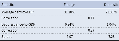

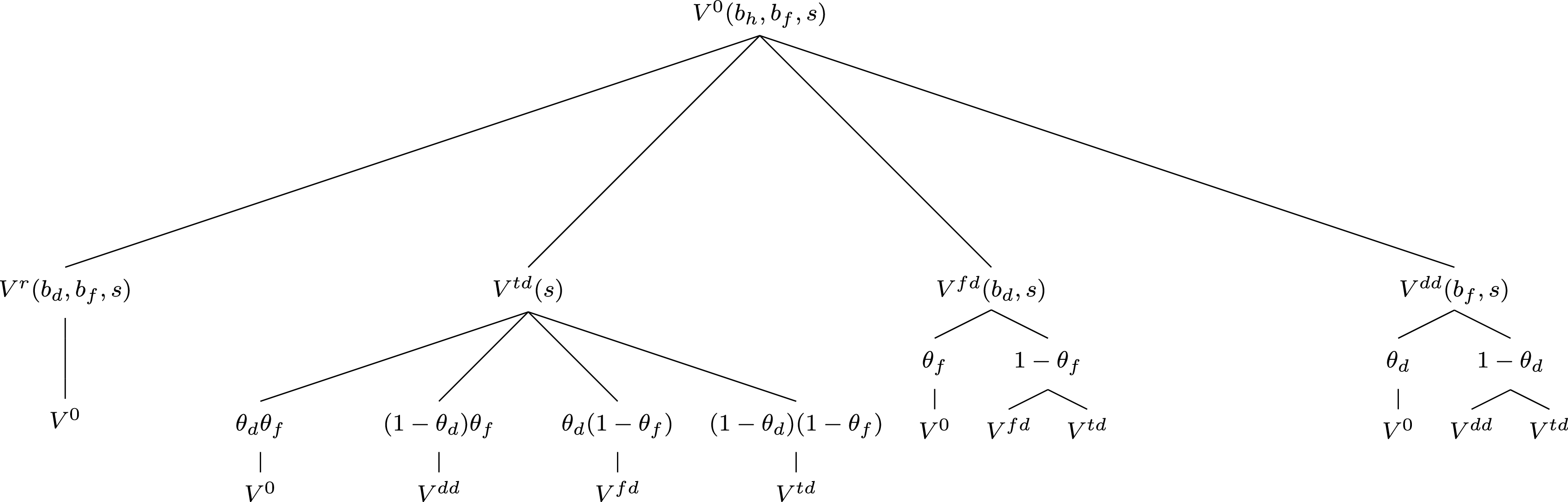


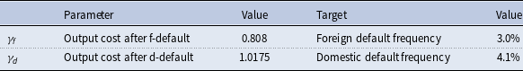


 Open access