

3.1 This Chapter’s Plan
I argued in Chapter 2 that experiencing work in an observatory control room develops students’ abilities to use observational data competently. But nobody expects that, by visiting an observatory for a few days and nights, they would become members of its staff’s community and culture. By contrast, educating PhD students aims at making them competent members in the community and culture of a science. This process takes much longer than a few nights in the control room. In this chapter I examine how Nadine, the PhD student we encountered in the Introduction, was instructed to tackle a common, often challenging problem: calibrating a new dataset and combining it with data from a different source for analysis. By following her around over two years as she achieved this goal, we learn how she became a competent member in the community and culture of extragalactic astronomy, not the least by being an explorer of social norms. Conversely, we gain insights into what makes combining scientific datasets often so challenging. As such, this chapter applies the tactics of Chapter 2 – take a problem of data-rich science, consider how it is “staffed” in a specific case, and follow its management ethnographically – to another setting.
I begin with reviewing graduate student training as a curious process in which instruction and the advancement of science go together, introduce the setting of Nadine’s PhD project, and then follow it through four critical moments. This account of Nadine’s work will also serve as a starting point for Chapters 4 and 5, on uses of diagrams (Chapter 4) and mundane reason (Chapter 5) in scientific research with large datasets.
3.2 Instruction and Membership
Even a casual visitor of a research setting notices that science is replete with situations of training and instruction. PhD students did almost all the data processing that I witnessed during my study. Of course, there is a lot more instruction in science than educating students. Scientists and technicians of all ages and career stages are taught how to use new instruments, new data, new computer code, and yet unfamiliar diagrams. Not all instruction is face to face. Far from it. Written descriptions and manuals instruct, too. But except for a few independently working postdoctoral scholars, every scientist at the Institute found themselves at one end or the other of one or more instructional relationships.Footnote 1
In PhD projects, training students and advancing science go together.Footnote 2 At the Institute, supervising bachelor and master thesis projects was often delegated to junior scientists, including PhD students and postdoctoral scholars. By contrast, PhD students were typically supervised by senior scientists, including the Institute’s directors. Senior scientists told me informally that good PhD students offered a better return on investment into their training than master students, who, they declared, need more guidance. Typically, three years long and with defined objectives, PhD thesis projects are important units in the organization of many collaborative projects.Footnote 3
Finishing a PhD is often understood to be more than acquiring certain skills, completing data analyses, and writing up a thesis, followed by the award of formal credentials. Ideally, it also signals the achievement of membership in a community and culture.Footnote 4 Doing so entails being able to accommodate to this social world’s normative expectations, epistemic and social orders, and social accountabilities. David Kaiser (Reference Kaiser and Kaiser2005, 1) argued that “scientists are not born, they are made.” I would add that they are made by doing science.
Witnessing unfolding PhD projects provides ethnographers both with an opportunity and a difficult challenge. It is an opportunity because not only is the position of an onlooking learner already defined (for students), it may be filled also by ethnographers, who can thereby witness acts of instruction. In the process, ethnographers can learn about researchers’ implicit, backgrounded assumptions. But doing so is challenging, since one does not achieve membership in a community and culture overnight, but over years. Scientists’ PhD projects take as long social scientists’ PhD projects and research grants. This makes it difficult for ethnographers to document and analyze this process. To make sense of it, ethnographers may also need substantial expertise in the work they witness.
Given these difficulties, social studies of PhD student education in science have relied mostly on interviews. Thus informed, Sara Delamont and Paul Atkinson (Reference Delamont and Atkinson2001, 88) argue that the “replication of science in undergraduate years (…) constructs a domain of relative stability,” whereas “doctoral students discover that ‘real’ science is more complex, and that failure is a normal outcome of routine work.” Once mastering their work, however, successful PhD students “remove all mention of the context, of the messy realities and of the tacit” from their publications (Delamont and Atkinson Reference Delamont and Atkinson2001, 89). Other interview-based studies refine, qualify, and supplement this picture.Footnote 5
Wolff-Michael Roth and G. Michael Bowen (Reference Roth and Bowen2001) note in response to Delamont and Atkinson (Reference Delamont and Atkinson2001) that interviews give us insights into how interviewees account for their experiences retrospectively, but they do not tell us reliably how interviewees have mastered their skills in the real time of practice. As a counterpoint, Roth and Bowen present an ethnographic account of how an advanced undergraduate student in field ecology learned to generate and analyze data in an independent research project. In her insightful ethnography of dendrochronologists, Meritxell Ramirez-i-Olle (Reference Ramirez-i-Olle2020) follows a PhD student through his project, but she does not make his learning experience her topic. Ethnographic studies of PhD student learning remain rare, and they typically focus on brief moments of interaction. Thus, Morana Alač (Reference Alač2011) uses video recordings to study multimodal interactions in graduate student instruction in neuroscience, whereas Philippe Sormani (Reference Sormani2014) combines a self-study, as an ethnographer, of using laboratory equipment without in-person instruction with an account of a PhD student’s discovery work in experimental physics. This chapter aims to complement these studies by witnessing a PhD student’s training over two years. It follows Nadine around as she mastered a common, often challenging problem: combining data from different sources for analysis. I shall argue that her achievement of membership hinged on this success.
That the successful instruction of science students goes along with their achievement of membership is a point that Ludwik Fleck and Thomas Kuhn made long ago. Fleck (1979 [Reference Fleck1935], 141) observed that junior scientists’ “thought style” appears to them as “natural and, like breathing, almost unconscious, as a result of education and training as well as through [their] participation in the communication of thoughts within [their] collective.” Kuhn insisted that students generate meaning not solely by comprehending statements (propositions) but through extensive practice, particularly when dealing with exemplars – “concrete problem-solutions that students encounter from the start of their scientific education (…) that (…) show them by example how their job is to be done” (Kuhn Reference Kuhn1970, 187). Communal practices are founded on exemplars. Training to be a scientist is not altogether different from learning a craft as an apprentice. It is a form of socialization – and thereby of the “reproduction of social worlds” (Macbeth Reference Macbeth1994, 312) – that may be necessarily dogmatic. Seeking to unite Garfinkel’s and Kuhn’s insights on education, Mary Douglas (Reference Douglas, Douglas and Hull1992, 244) adds that exemplars must be “used in regular procedures of accountability” to be effective in founding collective beliefs. She notices that “puzzle-solving techniques are prime in the process of community creation” (Douglas Reference Douglas, Douglas and Hull1992, 244).
However, these studies do not tell us how “procedures of accountability” are engaged sequentially in creating new members. Thus interested, I am inspired by an unusual source for the social study of science: Lawrence Wieder’s (Reference Wieder1974) ethnography of the “convict code” in a halfway house for released ex-convicts. The halfway house that Wieder studied was meant to prevent convicted narcotics offenders from relapsing into new offenses upon their release from prison. Wieder discovered that its convict residents kept referring to a loose set of maxims by which residents ought to abide, for example, not to “snitch” – that is, not to display cooperation with the halfway house’s staff. What Wieder came to call the convict code also included references to types of people – such as “kiss asses” and “snitches.”
Wieder recognized that this code, although never specified in detail (and never in writing), was familiar and binding to both the halfway house’s residents and staff. New residents and Wieder, as their ethnographer, had to familiarize themselves with it by using what Garfinkel (Reference Garfinkel1967, 78) called a documentary method.Footnote 6 As if provided only with fragments of a document, new residents and staff members (as well as the ethnographer) had to draw on what they experienced to make informed guesses for how to act in yet unfamiliar circumstances. They did so by witnessing long-term residents’ reactions and learned about the “convict code” by entering into its domain of accountability. The code became a collection of “embedded instructions for perception” (Wieder Reference Wieder1974, 203) that was used reflexively: it was “a constitutive feature of the setting [it made] observable” (Garfinkel Reference Garfinkel1967, 8). The code and its enactment are instructive for linking learning and discovery to the achievement of membership in science. Wieder’s study points to a convergence of ethnographic practice and doing science that I have pointed out already in Chapter 2.
3.3 A Domain of Practice: Photometric Redshift Surveys of Galaxy Evolution
Nadine’s PhD project brought her into a research group known for innovative studies of cosmological deep fields: small parts of the sky selected for offering views of the distant universe to study galaxy evolution. Since early in the twentieth century astronomers have been using the finite speed of light as a “tool” for studying galaxies’ distant past by observing faraway objects (Peebles Reference Peebles2020). Assembling a chronology of their evolution requires knowing the distances to many galaxies. What astronomers call redshift (abbreviated as z) is a measure of distance. It indicates how much the wavelengths of the light emitted by cosmic objects are stretched due to cosmic expansion, shifting specific spectral features to longer wavelengths. Introductory textbooks describe how redshifts are measured with spectrograph equipped with a glass prism or grating to disperse incident light into its constituent wavelengths (Chromey Reference Chromey2010). For the study of large samples of distant galaxies this technique is limited due to the prohibitively large amount of telescope time needed to record the spectra of faint galaxies one after another. This hindered statistical studies of galaxy populations.
In the late 1950s, William Baum proposed a way to circumvent this problem. By taking photographs through a variety of color filters, he was able to construct low-resolution spectra of several galaxies per field of view and estimate the redshift of prominent spectral features by comparing these with the template spectrum of a nearby galaxy (Baum Reference Baum and McVittie1962). At the price of a decreased spectral resolution Baum could measure many “photometric redshifts” in a certain amount of telescope observing time. When sensitive large digital detectors became available in the 1980s and 1990s, this technique was taken up and developed by several researchers who improved the template-fitting technique. While promising, redshifts inferred from such “multicolor” observations remained controversial for several years, largely because of occasional “catastrophic outliers” (Koo Reference Koo, Weymann, Storrie-Lombardi, Sawicki and Brunner1999).
In 1999, the MAMBO (pseudo-acronym) team (see the Introduction) set out to improve photometric redshifts by modifying earlier work in three ways. First, they decided to use seventeen filters instead of the five to seven that researchers had typically used. In the new project, five filters were “broad-band” filters covering the visible spectrum from blue to red evenly. The other twelve were “medium-band” filters covering the same spectral range in a more fine-grained way. Thus, instead of one orange filter there were now three filters transmitting different hues of orange light. For measuring photometric redshifts, medium-band filters had not been used before in a systematic way. Second, the team built the Wide-Field Imager (WFI), a new charge-coupled device camera for the 2.2-meter telescope at La Silla Observatory in Chile, to which they had privileged access through their home institute. This camera’s wide field of view allowed recording the light of many objects in every single exposure. Third, they improved the fitting technique by developing a digital template library of a large set of galaxy types, as well as of stars and “active galactic nuclei” at various redshifts.Footnote 7 Observing five fields in the sky, the MAMBO team produced by 2003 a catalog of 25,000 galaxies up to redshift one, corresponding to a lookback time of half the universe’s age. This sample of distant galaxies was ten times larger than any other available at this time (Lin et al. Reference Lin, Yee and Carlberg1999).
When I began my ethnographic study of the MAMBO project in mid-2007, work on the survey proceeded in two directions. First, to detect more distant galaxies whose spectral light is stretched to longer wavelengths, the team added near-infrared observations of three of the five fields, using a new camera attached to the 3.5-meter telescope of Calar Alto Observatory in Spain. Second, they constructed an improved template library of simulated galaxy spectra for the purpose of extending the spectral range from optical (visual) wavelengths to the near infrared. This was meant to make template fitting feasible for more distant (higher redshift) objects in the new observations and to obtain more precise clues about their physical properties.
3.4 Four Reflexive Moments in Nadine’s PhD Project
In 2005, MAMBO team members had begun supplementing an existing (optical) dataset from La Silla Observatory in Chile with new (near-infrared) observations at longer wavelengths taken at Calar Alto Observatory in Spain. They wanted to extend the survey’s outer limit from redshift z = 1 to z = 2, covering the last 9 billion years. Obtaining a sizeable sample of several thousand distant galaxies and using it to trace statistically how the colors, luminosities, and masses of galaxies have evolved over this period was to be Nadine’s PhD thesis project.Footnote 8
Recording and calibrating data to assemble a catalog – a table of measurements and estimated information – was at the heart of Nadine’s project. Patrick, a postdoctoral researcher who was already familiar with template fitting, summarized the data-reduction and analysis tasks that lay ahead of her in the form of a recipe:Footnote 9
The first thing is to upload the exposures … check the FITS headers and do all that. (…) The next steps are bias subtraction … correcting for nonlinear effects and some other small tidbits … making the flat field … divide all science images by it (…) and correct for cosmics. (…) Then comes the photometry. If you have made a catalog already with SExtractorFootnote 10 and know where the galaxies are on your exposures … you do the photometry in each filter (…) meaning that you have to determine the instrumental magnitudes at these positions … and then calibrate all of that (…). At the end you have magnitudes … normal magnitudes … and those are plugged into the multi-color classification. For that you first have to calculate colors (…) and they all go into the classification where you use the colors to decide not only what kind of object it is … but also at which redshift it is … and when you have the redshift and the object type and spectral type you can derive other parameters … like mass … total luminosity and the like (…). The data are stored in tables … and they tell me … star number 1828 has got 18 counts per second in this image taken with this filter … and this information is saved in a large table … which is created when instrumental magnitudes are computed … and you keep working with these tables (…).
Patrick describes this progression from “raw data” to calibrated data as a single sequence of tasks,Footnote 11 much as it is commonly described in the methods sections of research publications.Footnote 12 One of the last steps in this sequence is to use a cosmological model to convert redshifts to distances and convert measurements to absolute, distance-independent values.
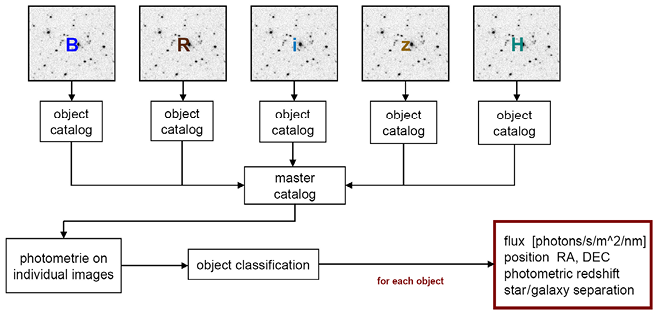
Team members used a flowchart to depict how their work proceeded from locally specific records to claims about physical objects and phenomena (Figure 3.1). Drawing on Patrick’s account and using material from Nadine’s work, I add specific detail in Figure 3.2.
Flowchart of the MAMBO research group’s data reductions as taken from a conference presentation of one of its members. It depicts the work as a sequence of operations. First, a set of exposures is taken of specific selected fields in the sky through a series of color filters (B, R, I, z, H). These are then used to algorithmically detect objects, take photometric measurements at the object positions, and classify objects by identifying the best-fitting match from a library of template spectra. The results are object positions, radiation flux densities, classifications of the object type (star, galaxy), and estimates of the photometric redshift, a measure of cosmic distance.
Note: The online version shows the colors of the original figure.
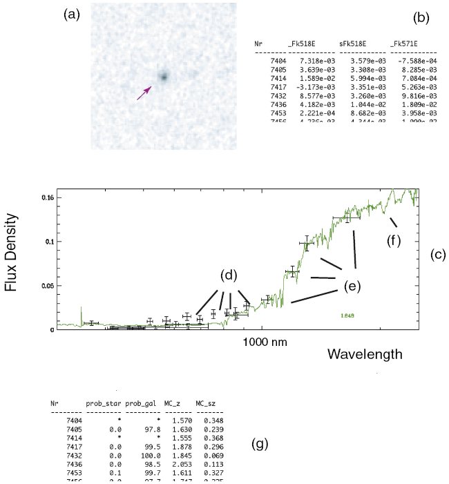
Scheme depicting basic steps of the MAMBO team’s spectral energy distribution template-fitting technique. First, exposures taken through each color filter are processed and calibrated with standard data-reduction procedures (a). In the resulting images, objects are detected algorithmically and assigned catalog numbers, their fluxes are measured, converted into magnitudes, and saved in a table (b). These can then be plotted as a spectral energy distribution (c), wherein measurements taken with the telescope in Chile (d) join those taken with the telescope in Spain (e). Crosses indicate measurement errors. Next, the best-fitting spectral energy distribution template, shown here as a continuous line, is selected algorithmically from the template library (f). Using the best-fitting template, the object is classified as a “star” or “galaxy,” and, in case of the latter, its redshift and physical parameters, such as mass and luminosity, are inferred from this fit and entered in the catalog (g).
Note: The online version shows the colors of the original figure.
In the following, I shall give an account of how Nadine’s work unfolded over two years, focusing on four episodes in which the sequential following of protocols became problematic. For this description it will be useful to employ Trevor Pinch’s (Reference Pinch1985) notions of “externality” and “evidential context.” They allow us to compare practices of data production and use across disciplines.
Trevor Pinch (Reference Pinch1985) notes that observational reports in physics are contingent on chains of inference, and this affects how they are assessed. He examines how a claim about the number of neutrinos emitted from the solar interior was made. As neutrinos hardly interact with matter, it is very difficult to detect and count them. The team running the experiment that Pinch describes placed a large tank in a deep underground mine to shield it from terrestrial and cosmic radiation and filled it with tetrachloroethylene (dry-cleaning fluid). When neutrinos hit chlorine atoms in the tank, these turned into atoms of radioactive argon. Once a week the tank was flushed to detect radioactive decays and record them with a chart recorder. The team then used the recorded wiggles to estimate the amount of radioactivity produced. After subtracting a background signal (ascribed to radioactivity from the subterranean environment), they converted the measured amount of radioactivity into the number of chlorine atoms hit, and this in turn to the number of neutrinos that had entered the tank. Researchers subsequently attributed the detected neutrinos to have come from the solar interior and not from other cosmic sources.
Pinch notices that the chart recorder’s wiggles were uncontroversial, but uninteresting for anyone except the research team’s members. As an observational report, these wiggles were of what Pinch called “low externality” – tied to their specific, local context – and “low evidential significance” – themselves not supporting interesting or risky knowledge claims. It was only by adding a series of assumptions that team members were able to claim that they had detected neutrinos from the sun. Freed from specific local details, their report was now of “high externality” (Pinch Reference Pinch1985, 13). As such it was suited to address evidential contexts of “high evidential significance,” of interest to researchers studying the solar interior, theories of gravitation, and climate change on Earth (Collins Reference Collins1992).Footnote 13
Two aspects make Pinch’s notions particularly salient for examining research with diverse datasets. First, as Steven Shapin (Reference Shapin1995, 265) observes, moving up along the “axes” of externality and evidential significance can be seen as taking a “credibility risk”: “critics can pick away at the gap between elements in the metonymic relationship,” but data makers can also “bid for rich credibility-rewards.” Shapin argues that this offers “a framework for describing the moral economy of risk and reward in the relevant community” (Shapin Reference Shapin1995, 265). Second, as I show in this chapter, members engage evidential contexts and their diagrammatic representation as contexts of accountability. Diagrams are cultural resources that become meeting places of epistemic and social action. What is negotiated in their use commonly retroacts on data calibrations and interpretations (see also Chapter 4).
3.4.1 Galaxies That Are “Too Bright for Their Distance”
In September 2007, eighteen months into Nadine’s thesis project, the new dataset consisted of about 1,300 near-infrared exposures taken through three medium-band filters and one broad-band filter (the so-called H band). Using pipelines, semi-automated computer code that senior team members had developed to process telescopic exposures, Nadine removed biases and dark currents, divided science exposures by flatfields, confirmed the detector’s linear response, and applied algorithms for removing cosmic ray hits. She then brought all images to a common point spread function,Footnote 14 a requirement for making the photometric measurements in different exposures comparable and combinable. Nadine considered this task accomplished when Otfried told her that the output images were “looking fine.” He encouraged her to proceed to measure the near-infrared fluxes at the positions in the field where objects had been detected in the previous optical imaging.Footnote 15
After Nadine ran the photometry algorithm and generated a first catalog (a table of the flux measurements of objects previously detected in the optical exposures), Otfried explained how to apply the template-fitting technique to the combined optical and near-infrared dataset. Using it so resulted in a table that listed for each object the best-matching template, object class (star, galaxy, quasar), photometric redshift, and – in case of galaxies – luminosity and mass (see Figure 3.2g). Thus equipped, Nadine’s study had gained in externality.
Most entries in the new catalog seemed inconspicuous, but a few dozen objects that had been previously classified as relatively nearby galaxies were now identified as bright and massive, distant galaxies at redshift 1.8 or so. Nadine was intrigued to find such objects. But while accepting that Nadine had done everything as instructed, Otfried remained noticeably reserved. He was puzzled by how bright the objects appeared given their distance and suggested they discuss her work at the next team meeting. In preparation for this, Otfried asked Nadine to make a set of plots, including a graph showing the old versus the new redshift for each object (i.e., the ones based on optical-only data versus those based on optical plus near-infrared data), as well as the spectral energy distributions of objects now reclassified as high-redshift galaxies.
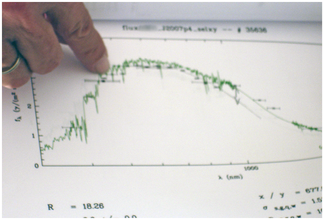
Otfried opened the meeting by presenting and describing Nadine’s plots, focusing on how the new template fits differed from those derived from the optical-only data (Figure 3.3). He noticed an offset between the near-infrared and optical magnitudes and suspected that it had caused the template-fitting code to pick wrong templates. He thus regarded the combined dataset as erroneous.
At a team meeting, Otfried is concerned about an offset visible in some galaxy spectral energy distribution fits that Nadine had prepared. This diagram depicts measurements of flux density over wavelength for one of these galaxies. As in Figure 3.2, dots with error bars represent the measurements and the continuous line represents the template model.
Note: The online version shows the colors of the original figure.
Within a few turns the conversation largely became an exchange between Otfried and Otto, who had overseen the construction and calibration of the near-infrared camera used for the new observations. Both were concerned about Nadine’s plots and debated them in light of their previous observing experience. Long before Nadine had joined the team, Otfried and Otto had struggled with what turned out to be straylight in the WFI at the 2.2-meter telescope. This had resulted in a troublesome flatfield that corrupted all flux measurements. Otfried surmised that Nadine’s result implied that this old problem had not been fully resolved.Footnote 16
At this point several options seemed possible. Nadine’s dataset comprised observations in twenty-one filters, recorded with two cameras attached to telescopes on different continents over seven years. Otfried and Otto knew that neither the cameras nor the telescopes would remain entirely stable over such a long period. But how could this be checked? Aware that the deep field Nadine studied is in a part of the sky that the Two Micron All Sky Survey (2MASS; Skrutskie et al. Reference Skrutskie, Cutri and Stiening2006) had observed previously, Otto suggested comparing the new observations with this survey’s photometric catalog, which was freely available on the internet. Many astronomers regard 2MASS as a reliable source of object positions and near-infrared photometry.
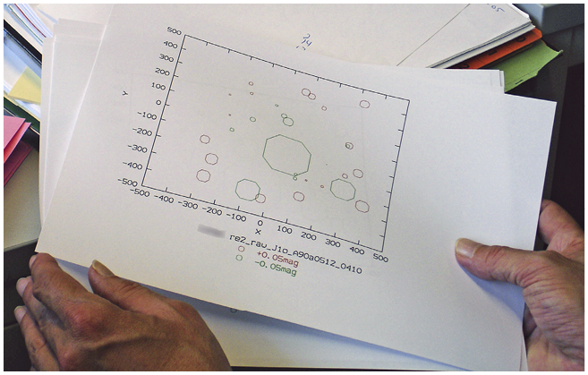
Prior to this discussion, Otto had written a computer program to compare the new photometry with entries in the 2MASS catalog. Within two days of the team meeting, Nadine managed to download the 2MASS data and used Otto’s program for preparing a diagram visualizing the differences in the fluxes of stars measured at various positions on the images. While the fluxes appeared to agree in the image’s center, there was a marked offset in a ring-like shape around it (Figure 3.4). To Otto and Otfried this suggested that they were dealing with an artifact in the new data, possibly due to stray light in the camera. Otfried concluded:
Following the group meeting, Nadine and Otfried assess the flatfield frames visually.
Note: The online version shows the colors of the original figure.

I think … what we have to do is to remove the ring … and see whether what comes out then is good enough. The problem is that we have something which is now … we had something which is clearly not good enough. We had objects which do not exist. I mean … the redshift two galaxies of twenty-first or twenty-second magnitude which clearly indicate that we have a problem … which is too bad … which is worse than what we can accept.
Here “magnitudes” is a measure of how bright objects appear on the sky and “redshift” is a measure of the distance to cosmic objects. Otfried implies that, at a certain distance, galaxies can only be that bright to be proper members of their class. Linking the brightness of galaxies to their distance is a statement about the universe’s geometric structure and light propagation in it.
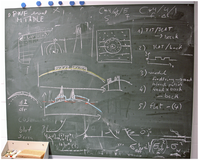
Using Otto’s code and the 2MASS catalog, Nadine, Otfried, Otto, and Patrick went on to quantify the excess light in the flatfield image (Figure 3.5). Following a series of discussions at blackboards, and while regarding paper printouts, they developed a recipe for subtracting the ring from the flatfield image (Figure 3.6). Nadine then used the corrected flatfield image for reducing all 1,300 raw exposures. After she had rerun the photometry and template-fitting codes, the presumed excess of massive galaxies at redshift 1.8 had disappeared.
Guided by Otto, Nadine assesses the flatfield frame quantitatively by plotting differences of her brightness measurements of stars in the field with those of the public 2MASS catalog.
Note: The online version shows the colors of the original figure.
Summarized on Otto’s office blackboard, a group discussion yields a recipe to correct for the flatfield ring that is now considered an artifact due to scattered light in the infrared camera. A sequence of arithmetic operations to the flatfield frames specifies its remedy (steps 1 to 5, as seen on the right).
Note: The online version shows the colors of the original figure.

By progressing from calibrating “raw data” to revealing astronomical phenomena, Nadine had gone from a context of low evidential specificity (Pinch Reference Pinch1985) – detecting faint light sources and measuring their brightness – to a highly specific, and perhaps risky, epistemic claim: identifying these sources as distant, massive galaxies. She had to go to a higher externality to be able to “lose the phenomenon” (Garfinkel Reference Garfinkel and Rawls2002, 264). At lower externality there were no phenomena to be lost. Individual traces of light in the exposures that Nadine worked with were never “just these traces,” but were – if epistemically productive – accountable to a galaxy’s spectral energy distribution, whose further constituent traces were revealed in the dataset’s other images.Footnote 17
Otfried and Otto made educated guesses about how reflections on lenses and glass filters in the camera might cause straylight in its images, but neither they themselves nor the observatory’s engineers attempted to find a quantitative physical explanation for it. These astronomers seemed interested only in being able to correct for the excess light recorded in the flatfield exposures computationally, a task for which access to the 2MASS proved valuable. The ring-like feature in the flatfield images thus became accountable not to a physical description of telescope and camera, but to the documented record of astronomical observations available to all researchers through the internet. For Otfried and Otto, making the artifactual ring (and, by implication, the camera’s performance) accountable to a “globally” stabilized catalog such as 2MASS appeared to be more secure and convincing than making it accountable to a local calibration. Indexical cues in the local setting thus triggered team members to recruit a wider set of accounting practices into their project. Until discovering the ring-like feature in the near-infrared exposures, both constituent digital datasets were regarded as equally malleable, being subject to possible correction.
3.4.2 An Overdensity of Galaxies That “Cannot Exist”
In the previous episode, Nadine had worked with the team’s “old” catalog of objects detected in optical wavebands. It lacks objects detected exclusively in the four newly observed near-infrared bands and thus misses the more distant objects that her project was searching. Rather than resolving the straylight issue to its possible conclusion, Otfried considered the flatfield images as “good enough for now.” He was now eager for Nadine to prepare a near-infrared selected galaxy catalog. In making this catalog, Nadine did everything as instructed. But again, a surprise ensued. In late 2008, when I was traveling abroad, she wrote to me, in an email message,
I would like you to be here to share our amazing discovery. I still have to convince myself to believe it. I have discovered a very high number (around 100) of red massive galaxies at [redshift] z around 1.6! We did check if it was a problem with the library but the SEDs [Spectral Energy Densities] look very good! I think that the library is good. We still have to calculate the mass for these objects, but they look massive. I don’t see obvious clustering, those galaxies are sparse across the field.
When I returned to the Institute, I learned that old-timers had done all “diagnostic work.” Nadine had not been involved. Otfried explained to me:
At first I thought that there really is something there … an overdensity at a redshift of 1.6 in our field. But then … discussing this with Oliver ((another old-timer)) convinced me that this has to be nonsense. First … you cannot expect such an overdensity to exist … and secondly … how these objects are distributed in the field … they are all over … and a ((galaxy)) cluster … even a supercluster (…) would cover only a fraction of our field if it were at a redshift of 1.6. Then you would see it as an overdensity ((in celestial coordinates)). (…) So I had to admit that it would be mistaken to assume that there is an overdensity … as it now seemed to be obviously wrong … if you like. And after a while I realized that the overdensity may be due to the asinh magnitude producing wrong colors.
As in the first episode, the plausibility of Nadine’s analysis was assessed with respect to the phenomena that template fitting revealed, such as “overdensities of objects” or “superclusters” of galaxies. The apparent overdensity – a clustering of objects in a part of the field – emerged after combining the two datasets. The optical-only dataset alone had not revealed it. Otfried realized that template fitting is sensitive to how one computes so-called color indices, which, in turn, depends on how one defines and measures magnitudes.
Astronomers commonly define magnitudes as a logarithm of the incoming radiation flux and color indices as the difference of two magnitudes pertaining to two wavebands (Chromey Reference Chromey2010, 27). In the MAMBO system, templates are fitted (and redshifts measured) in color space, that is, by comparing sets of observed color indices with those derived from the template library. However, for faint objects at the noise limit of an exposure, magnitudes and color indices become ill-defined due to the asymptotic behavior of the logarithm of near-zero arguments. Other astronomers had tried to remedy this problem by introducing a modified magnitude definition that uses the inverse hyperbolic sine (asinh) instead of the logarithm. This function resembles the logarithm for small fluxes, but is “better behaved” for small positive arguments.Footnote 18 Various astronomical survey projects, including MAMBO, adopted these “asinh magnitudes.”
Alerted by Oliver’s concern with the overdensity at redshift 1.6 being implausible cosmologically, Otfried suspected that this modified magnitude definition might produce artifacts when applied to the MAMBO filter set because of its combination of broad-band and medium-band filters. For an object that has been detected in a broad band, but is too faint to be detected in a medium band, spurious color indices can result, making the algorithm pick the wrong template. Specific combinations of wrongly assigned color indices can make the algorithm preferentially select templates with a specific redshift for a range of spectral energy diagram shapes, resulting in what some practitioners call “redshift focusing.”
After some experimenting, Otfried arrived at a new definition for computing magnitudes at low signal-to-noise ratios that seemed to “behave well” for color indices derived from combinations of broad- and medium-band photometry. For brighter objects, this definition converges with the traditional logarithmic magnitude definition. After Otfried had included the new magnitude definition into the MAMBO photometry algorithm, it became Nadine’s task to recalculate the photometry for all objects in all filters. Using these to run the template-fitting algorithm again made the overdensity of galaxies at redshift 1.6 disappear. It was now considered an artifact.
As in the first episode, it was the perceived implausibility of a finding at presumably high externality – a statement about a large-scale structure in the distant universe – that prompted a return to lower externality and a less specific evidential context. However, in this instance, accounting practices were not cast wider than before, but local procedures were refined to enable an intertwining of astronomical phenomena, observing procedures, and reduced digital data.Footnote 19
3.4.3 A Luminosity Function That “Nicely Agrees”
Nadine’s next task was to assess whether her new measurements could reproduce published statistical findings about distant galaxies that other teams had made. Otfried now asked her to prepare a galaxy luminosity function, a graph depicting the number of galaxies in a specific volume as a function of galaxy luminosity. Such graphs are commonly used for inferring evolutionary changes in the galaxy population statistically.
Equipped with widely used recipes and aided by Oliver, Nadine wrote computer code for preparing luminosity function diagrams from the combined catalog. After considering her work, Otfried complimented Nadine by saying that her diagrams “look okay.” He then pulled out a paper copy of an article that a team of US astronomers had recently published. This team of renowned scientists had assembled luminosity functions derived from several deep fields at different parts in the sky in one plot, including one they had made using earlier data released by the MAMBO team. Working with pencil and ruler, Otfried copied measurements from Nadine’s plot to the published graph and then held printouts on top of each other against the light to assess these diagrams’ “sameness” or “difference.” Thus, he noticed a systematic offset between the graphs that puzzled him and asked Nadine to check carefully what she had done, concluding that “if it is not too far away from what everyone has found I would be happy.” Within a day Nadine noticed that she had introduced an erroneous factor of two in adopting the software code. Remedying it made both plots “agree quite nicely,” as Otfried declared upon further visual inspection.
By preparing the luminosity function, Nadine again moved to work at higher externality where a concern for individual objects gave way to considering the statistical properties of the galaxy population and its evolution. Unlike in the previous cases, accounting practices involved manual craftwork in addition to the visual assessment of “reasonable agreement” (Kuhn Reference Kuhn1977, 185) with existing data or representations of previously established phenomena. Comparing Nadine’s work with that of well-known and respected astronomers who drew on the same data, and finding them to be in reasonable agreement, raised Otfried’s trust in Nadine’s computations and made both datasets accountable to the work of these other scientists.Footnote 20
3.4.4 A Troubling “Hole in the Universe”
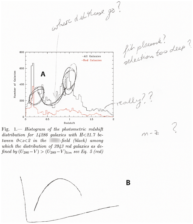
A few months later, after Nadine had defended her PhD thesis, she had finished a draft journal manuscript describing her work. When Peter, a former PhD student of Otto’s who had been instrumental in developing and conducting the MAMBO survey, visited the Institute they met with Otfried to discuss the manuscript. Nadine’s draft included several graphs that the described the galaxy sample. The first of these was a histogram showing the number of objects (n) as a function of redshift (z), a so-called n(z) plot (Figure 3.7).Footnote 21
Histogram in Nadine’s draft manuscript, showing the number of galaxies as a function of redshift for all objects detected in the A2713 field. This printout includes Peter’s handwritten notes as made prior to the group meeting (unlabeled) as well as the marks he added during the discussion with Nadine and Otfried as described in the text (labeled A and B).
Note: The online version shows the colors of the original figure.

This histogram’s shape troubled Peter. He doubted it was cosmologically plausible and suspected that it hinted at a bias in their sample’s faint end, where it would be more complete for bright galaxies of a certain color or shape. Otfried agreed with Peter that the graph is accountable to what the distribution of galaxies in the universe is like, but he disagreed about what this implied for its shape. He argued that the dip seen in the diagram between redshifts 0.3 and 0.9 documents a dearth of galaxies in the appertaining distance interval, a “hole” in the universe.Footnote 22
In the discussion that followed, Peter used his laptop computer to generate additional plots from the data. These showed how a change in the faint magnitude limit affects the histogram’s shape. Otfried conceded that the sample’s degree of completeness did indeed vary with galaxy color and magnitude, that this was likely to cause the dip seen in the histogram, and that they had to redefine their galaxy sample. Otfried agreed that, after all, there seemed to be no hole at this part of the universe.
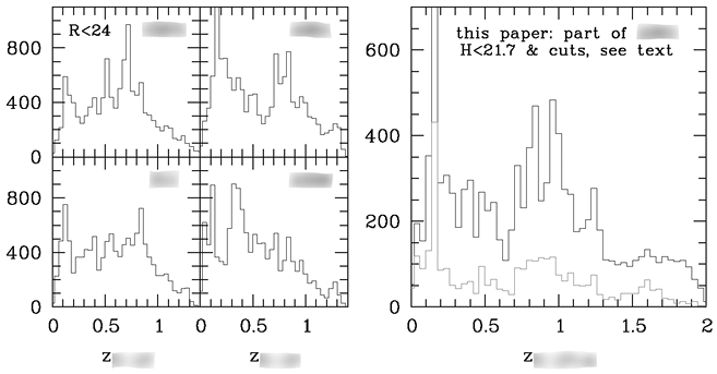
In this instance, in which two old-timers initially disagreed about “what the universe is like,” Nadine was not forced to return to work at lower externality. Instead, her task was to remove objects from her sample, starting with the faintest galaxies and progressing to brighter ones until obtaining a sample that was “reasonably complete.” Eventually, Otfried, Nadine, and Peter agreed to remove galaxies that were fainter than a limit magnitude that depended on the redshift, arriving at the sample that was subsequently used for the published analysis (Figure 3.8).
Revised histogram as it appeared in the published paper, showing on the right the number of galaxies as a function of redshift for all objects in the same field as in Figure 3.7, selected according to refined criteria from Nadine’s optical plus near-infrared galaxy catalog. The dip seen around z = 0.5 in the earlier version is less prominent due to the adoption of different selection criteria for the galaxy sample. On the left, four similar histograms are now included, each depicting one of four fields that the MAMBO team observed. These histograms use the “old” (optical-only) dataset. They illustrate “cosmic variance,” that is, how much the numbers and volume densities of galaxies vary when observed with the same technique in different parts of the sky.

3.5 Discussion: Instruction, Reflexivity, Membership
By following Nadine’s work over two years we get a sense of how she became a competent member in the community and culture of extragalactic astronomy. Conversely, we gain insights into what can often make combining new data with an existing dataset so challenging. As we have seen, astronomers describe this work as a single linear sequence of operations (Transcript 3.1 and Figure 3.1), but I witnessed that their practices were reflexive in an ethnomethodological sense, in that earlier steps of work were reassessed and modified, subject to the outcome of later steps in the sequence.Footnote 23 This prospective and retrospective reasoning engaged discipline-specific representational formats and contexts of accountability.
In the midst of her project, exasperated yet again from trying to run computer code for basic data reductions, Nadine once exclaimed: “My job is to get error messages!” At that time, her challenge was to run this code so that it would not crash but generate meaningful output. Two years later, after Nadine had defended her PhD thesis, I asked her how many times she had done the reductions of her dataset. She replied:
I don’t know … many times! From the raw frames to the fully reduced frames … and then many times the photometry … again and again and again! (…) I think that in astrophysics it never fits. You always need to use your knowledge to verify what you are doing. Every calculation. You have an idea how it can be … but you have to be very careful with all the details. And you have to verify each step to go on and continue with the recipe. And with each part of a recipe you have to see if there is any problem there … because the recipes are never perfect.
In this retrospective account, Nadine alludes to her experience of the unavoidable incompleteness of written instructions that always require researchers’ “ad hocing” (Garfinkel Reference Garfinkel1967, 22), that is, their on-the-spot use of contextual knowledge for making decisions that are “good enough for now.” She also hints at the necessary “willingness to wait” (Garfinkel Reference Garfinkel and Rawls2002, 202) in learning a practice. From despairing over troubleshooting computer code to engaging multiple contexts of accountability, Nadine acquired not only a sense of the limitations of rule-following, and of the reflexivity necessarily involved in working data together: considering their outcome, she learned to review and repair past actions. She mastered the task of proceeding from knowing about a cosmology to using it. And she discovered how critical well-calibrated data are to a scientific analysis.
What, then, about Nadine’s achievement of membership? In this discussion I approach this question by first specifying how images and diagram were constitutive of her team’s work. Then I characterize the domain-specific body of assumptions that team members used as a resource for achieving accountability. Eventually, I ask what its use implies for data calibration and the training of junior scientists.
3.5.1 Scaffoldings of Graphs, Contexts of Accountability
The documentary practices that constituted Nadine’s work involved a range of marks and inscriptions: telescopic exposures, spectral energy distributions, color–color plots of stars and galaxies, as well as galaxy color-magnitude diagrams, luminosity functions, and the n(z) plot (see Figures 3.3 and 3.7).
These diagram formats are conventionally used in astronomy for interpreting data in evidential contexts of increasing externality: a spectral energy distribution is made for individual objects, color-magnitude diagrams display measurements of many objects in a scatterplot (where individual objects are recognizable), whereas all individual object information is erased in luminosity functions, which describe populations of galaxies. In the work that I witnessed, these diagrams were not only constitutive of the phenomena observed, but were also engaged to provide contexts of accountability. Each trace that Nadine’s work revealed, that is, each flux measured in an exposure at a position where a signal had been detected algorithmically, was never “just this trace,” but was regarded as one of several constituents of an object’s spectral energy distribution that the dataset’s exposures revealed, all of which were made accountable to a library spectral energy distribution template.
A spectral energy distribution is often represented as a graph of radiation flux density (“intensity”) as a function of wavelength (cf. Figures 3.2 and 3.3). The team’s old template library consisted of a set of spectral energy distributions observed with a spectrograph. The new library’s templates were derived from computer simulations of the spectral light emitted from a model of stellar populations. They were made to match the old templates where these were available and extended the template library to longer wavelengths and higher redshifts. In this work, template fitting never is a comparison of “nature” with “models” but a comparison of the momentary endpoints of two different trajectories of documentary practices in the representational space of observational astronomy (cf. Rheinberger Reference Rheinberger1997, ch. 7). The templates – a kind of model – were a means to constitute phenomena from data and were thus used as tools to move from lower externality toward higher externality for addressing more general evidential contexts.
Note that, in this team’s work, contexts of accountability do not dwell in some abstract space but are defined by diagrams. Many of these are conventional and used by astronomers worldwide (Figures 3.3, 3.7, 3.8, and 3.9), but others are used only within the team (such as Figure 3.5). Diagrams essentially define contexts of accountability.Footnote 24 They are meeting places of epistemic and social action, as I will examine further in Chapter 4.
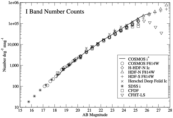
Journal articles accompanying the public release of deep field survey data often contain plots characterizing a new dataset and comparing it with existing ones. Number counts, showing the number of detected objects in a field (vertical axis) as a function of flux density or magnitude (horizontal axis), illustrate the degree of the datasets’ “sameness.” As such these diagrams assert and specify the reliability of new observations.

3.5.2 Cosmology as a Convict Code
When Otfried, Otto, Oliver, and Peter instructed Nadine, they used assumptions about the universe that they agreed upon or negotiated on using. They regarded galaxies at redshift 2 as “unlikely” to appear as bright as 20 mag, did not “expect” overdensities at redshift 1.6 to extend across the field of view under consideration, agreed that galaxy luminosity functions made from observations of different parts of the sky should look “more or less the same,” and argued about whether there is a “hole” in the “universe as we have known it before.” Otfried, Otto, Oliver, and Peter thus oriented to the observed world as having a single “underlying pattern” (Garfinkel Reference Garfinkel1967, 40, 78). This assumption informed their assessments when jointly regarding the diagrams that Nadine had prepared. Like the other PhD students they instructed, she was guided to apply a “documentary method” (see Footnote footnote 6) to elicit it.
Authors of research articles on galaxy evolution routinely make the cosmological assumptions they use explicit. In their “Introduction” sections, articles typically include a sentence which specifies the “cosmology,” such as
We use the standard Lambda cold dark matter (ΛCDM) cosmology with H0 = 70 km Mpc−1 s−1, ΩΛ = 0.70, and ΩM = 0.30.
or
Throughout this paper, we assume a Planck Collaboration et al. (2020) cosmology of H0 = 67.4 km s−1 Mpc−1, Ωm = 0.315 and ΩΛ = 0.685.
Here H0 (the Hubble constant), ΩM or Ωm, and ΩΛ (the fractions of matter and dark energy of what astronomers call the critical density) are three of six numerical parameters characterizing the world model that is currently dominant.Footnote 25 Both Patrick’s account of this team’s work (Transcript 3.1) and research publications on galaxy evolution suggest that astronomers use this cosmology and the parameters specifying it only to convert observed redshifts into physical distances and magnitudes into luminosities. Apart from contexts of instruction, these astronomers did not make the phenomenal properties of the sky and of stabilized astronomical phenomena explicit as resources for combining new and existing data. However, as seen earlier, references to these phenomena permeated the work that I witnessed. It is in this practical way that an “implicit cosmology” is used both constructively and descriptively as a shared view of “what the universe looks like” as seen through the representational (diagrammatical) formats of observational astronomy, a view that novices must learn to adopt. Thus understood, an “implicit cosmology” is a collection of “embedded instructions for perception” (Wieder Reference Wieder1974, 203), much like the “convict code” in the halfway house that Wieder described.
Wieder’s account resonates with Melvin Pollner’s study of mundane reasoning. Pollner argues that because of their mutual orientation to the assumption of an “incorrigibly objective and commonly shared world” (Pollner Reference Pollner1974b, 53) members of a practice can recognize and resolve disjunctive experiences (as they typically occur in the combination of datasets). In doing so, members commonly rely on ceteris paribus clauses.Footnote 26 Embedded in members’ reasoning, “incorrigible propositions” (Gasking Reference Gasking and Flew1955) are resources for reflexively preserving their own validity. As Pollner (Reference Pollner1987, 18) argues, “mundane reason is not an empirical version of reality but an a priori specification of its features in terms of which empirical claims are reviewed for their adequacy.” I explore this further in Chapter 5.
Nadine and her supervisors inferred the distant galaxy population’s properties through a sequential intertwining of data, phenomena, and equipment. In achieving this, the elements of their “implicit cosmology” remained stable. But is an “implicit cosmology” as stable as the convict code appeared to Wieder during his fieldwork in the halfway house? The fourth episode, where Peter and Otfried debated the existence of a “hole in the universe,” demonstrates that “sameness” is negotiable in light of what astronomers call “cosmic variance.” Theorists claim that the homogeneity and isotropy of the universe that the standard model postulates are realized on the largest scales only (Spergel et al. Reference Spergel, Verde and Peiris2003, 175). Whenever astronomers observe a small part of the sky (as they do when studying deep fields), the “sameness” of these fields with other small parts of the sky is not guaranteed outright but needs to be established empirically in the course of work. This is what Otfried, Peter, and Nadine did by including the left panel shown in Figure 3.8. It depicts the number of galaxies as a function of redshift in four distinct fields on the sky, illustrating the range of possible cosmic variation. In this way the reflexive use of an “implicit cosmology” is delimited in this inductive work.
As observational astronomy develops, the elements of a cosmology are incorrigible until further notice only.Footnote 27 Would revisions or refinements of the “implicit cosmology” affect astronomy’s social order, or have they done so in the recent past? For their practices to be mutually recognizable, astronomers need to work with a cosmology. Throughout the late twentieth century there was a notorious uncertainty among astronomers about basic cosmological parameters, dividing researchers, by and large, into two factions.Footnote 28 In 2003, the widely publicized release of observations taken with the NASA spacecraft Wilkinson Microwave Anisotropy Probe (WMAP) resulted in a set of precisely determined cosmological parameters that most researchers came to agree upon (Spergel et al. Reference Spergel, Verde and Peiris2003), ushering in what has been called an era of “precision cosmology” (Primack Reference Primack2005). Years after this release I heard researchers referring to it as “The Gospel according to WMAP.” By doing so they seemed to allude not only to its authority and hegemony, but also to the moral implications of mutually sharing an order of (and for) practice.
As it is through a cosmology that people consider the world as organized, this is where the astronomers’ cosmology meets the ones that anthropologists are more familiar with. It is through cosmology, anthropologist Michael Herzfeld (Reference Herzfeld2001, 194) writes, that “people treat the universe as organized: rather than a collection of random physical components, it is a highly ordered disposition of matter and energy structured in different levels of size and complexity.” A cosmology is not merely a set of beliefs, but also a resource for action. It defines a normativity that has epistemic and social uses. Or, as Mary Douglas (Reference Douglas1975, xix) put it, “[t]he known cosmos is constructed for helping arguments of a practical kind.”Footnote 29
3.5.3 Calibration
Patrick’s description of the team’s workflow (Transcript 3.1) and Otto’s diagram thereof (Figure 3.1) suggest that data calibration and analysis are two distinct parts of a project. But it turns out that they are closely enmeshed. As in physics, calibration in astronomy is often understood as the “use of a surrogate signal to standardize an instrument” (Franklin Reference Franklin1997, 31). In astronomical photometry, optical flux and color standards are derived from the star Vega (α Lyrae) as the primary calibrator, which is used to calibrate secondary and then tertiary standard stars all over the sky, whose fluxes are subsequently used as reference signals.Footnote 30
Up to her first run of template fitting, Nadine’s calibrations had proceeded in this way, but her calibration did not end there. Her work oscillated between making representations which could be interpreted as revealing phenomena at high externality and probing into the observing situation and data analysis where artifacts in the (malleable) data can be removed or analysis procedures corrected. Along this way these researchers replicated phenomena deemed already stabilized.Footnote 31
Astronomers argue that they subject reduced and calibrated data to specific evidential contexts solely to obtain a “sanity check” of the calibrations. They insist they do not “tune” them to make the data replicate known phenomena through enforcing their “sameness.”Footnote 32 As in the MAMBO team’s work, publications describing new observations of deep fields typically contain flux measurements of objects much fainter than those included in published (and stabilized) all-sky catalogs such as the 2MASS mentioned earlier. One means to assert and to demonstrate their reliability and trustworthiness is to represent them in a standard format along with observations of other fields that are deemed comparable. Galaxy luminosity functions (see episode 3) are such a format; diagrams of number counts, in which the number of detected objects in a field is shown as a function of flux density or magnitude, are another (Figure 3.9). They can be used to assess the similarity and difference of datasets visually. While cosmic variance affects and delimits “reasonable agreement” (Kuhn Reference Kuhn1977, 185) in either format, astronomers deem data that have “withstood” being subjected to such diverse evidential contexts as more reliable than data that have not.Footnote 33
Note, eventually, that engaging different contexts of accountability would have produced differently calibrated datasets, optimized, perhaps, for a better recognition of extended light or of galaxies that are merging, or for making measurements of weak gravitational lensing. In this way the researchers’ interests are imprinted in a dataset.
A common sentiment among the astronomers I talked with is that one should only release higher-level data (such as catalogs) that have been used successfully for a scientific analysis. Says a senior astronomer:
Another senior astronomer told me:
My lesson from being in the survey business is that it’s only when you do science with the data that you learn how good they are … or if there are problems with the data. Many mistakes appear only then.
“Doing science” in these views means successfully using data of relatively high externality to address specific evidential contexts. Note that neither of these two astronomers claim that a scientific result needs to be replicated for its constituent data to be releasable. Their point rather seems to be that researchers ought to inspect data and analyses for their “believability.”
3.5.4 Membership
At the beginning of her project, when she encountered unfamiliar representational spaces, Nadine could not know herself what to count as “same” and “different,” what was “good enough for now” and what had to be done differently.Footnote 34 Only after being exposed to various, diverse settings did she manage to share an order of, and for, practice, and make distinctions about sameness and difference with which members like Otfried, Otto, Oliver, and Peter agreed. Nadine’s achievement was not solely “cognitive.” Rather, with her becoming a user of a cosmology, cosmology’s domain of accountability was extended to her and her work. Figuratively, this domain was a “meeting place” of her actions and the actions of those who were inducted earlier at the Institute and at other sites of extragalactic research. For these members, a shared “implicit cosmology” has become a “guide to perception” (Wieder Reference Wieder1974, 74).Footnote 35
Nadine’s successful use of a cosmology is not the only indicator of her achievement of membership in the culture and community of extragalactic astronomy. I witnessed how she participated in group and seminar discussions and laughed upon hearing puns like Owen’s (Introduction, Transcript I.1). Over time I kept noticing moments when, for Nadine, “the implicit” could eventually remain unsaid and backgrounded. When entering the MAMBO research group, Nadine’s situation was not unlike that of an ethnographer entering a new field. Much of her learning happened without her noticing it, by immersing herself in a social setting. It included meetings with Otto and Otfried, discussions with Patrick and Peter, team meetings, lunch and coffee breaks, and travel to observatories and conferences. In various environments she had to learn how to ask questions and make practical sense of the responses she received.
I mentioned earlier that references to the reflexivity of accounting practices are characteristically absent in the methods sections of research publications. This includes the paper that Nadine wrote at the end of her work. Two years later, a new PhD student in the research group, who arrived after Nadine had gone, found it impossible to continue the calibrations and analyses that she had left behind straight away, but needed frequent consultations with Otfried, just as Nadine did early in her project.
It is tempting to define the achievement of membership in a scientific community as the achievement of becoming an author, a contributor to the scientific literature.Footnote 36 Episode 4 was part of this process for Nadine, but already episode 3 brought her data analysis in “contact” with the literature to which her paper was meant to contribute. Her data was about to become public along with her journal article or soon thereafter, and thus her work would soon be open to public scrutiny. That there is often no clear “correspondence relationship” (Sharrock and Anderson Reference Sharrock and Anderson1986, 58) between laboratory research and its description in a scientific article has been pointed out long ago (Medawar Reference Medawar1963). Early laboratory ethnographies dwelt on this and emphasized scientists’ “literary reasoning” (Knorr Cetina Reference Knorr Cetina1981, 94) for rhetorical and argumentative purposes, for the benefit of securing resources, and as part of the process of “fact construction” (cf. Latour and Woolgar Reference Latour1986, 75–88). While some forms of “literary reasoning” seem inevitable, the raised accountability of working with public data is bound to constrain data analyses and interpretations throughout a project, to which a journal article is reflexively tied.
As Nadine aspires to fulfill her dream of becoming a professional astronomer, her objective is biographical. As an author, her name is attached to her work, prompting her concerns over her reputation. In my account, reputation was alluded to only briefly in the third episode, where Otfried consulted an article published by respected colleagues to assess Nadine’s draft luminosity function, but scientists are obviously mindful of its significance and make decisions on its basis, as has been noticed in early sociological accounts and ethnographies.Footnote 37 As a visiting scientist at the Institute insisted, “science is self-correcting, but careers are not.” Reputation, as this episode suggests, is a resource for accounting practices in data-rich research.
While focusing on the achievement of membership, I began this chapter with proposing to apply the tactics of Chapter 2 – take a problem of data-rich science, consider how it is “staffed” in a specific case, and follow its management ethnographically – to a different case: the common challenge of combining scientific datasets. This brought the reflexivity of data reductions and analyses as well as its resources (such as contexts of accountability), all typically omitted from published reports, into view. Members’ social and cultural practices thus become scaffolds built into well-calibrated and well-combined datasets.


 Open access