


1. Introduction
Radio recombination lines (RRLs) are important tools for studying ionised gas. Kardashev (Reference Kardashev1959) first proposed the possibility of detect ing RRLs in H II regions, and RRLs were subsequently detected for the first time in the nebula NGC 6618 (Sorochenko & Borodzich Reference Sorochenko and Borodzich1966). RRLs have been widely used to trace faint and deeply embedded H II regions (Reifenstein et al. Reference Reifenstein, Wilson, Burke, Mezger and Altenhoff1970; Wilson et al. Reference Wilson, Mezger, Gardner and Milne1970; Anderson et al. Reference Anderson2015), which may correspond to distant massive star formation regions (Anderson et al. Reference Anderson2015). RRLs have also been used to detect the Galactic Warm Ionized Medium (Tanenbaum, Zeissig, & Drake Reference Tanenbaum, Zeissig and Drake1968; Dettmar Reference Dettmar1990; Rand, Kulkarni, & Hester Reference Rand, Kulkarni and Hester1990.
The maser effect of RRL was first predicted by Goldberg (Reference Goldberg1966), and the first Galactic hydrogen RRL maser was later identified in MWC349 (Martin-Pintado et al. Reference Martin-Pintado, Bachiller, Thum and Walmsley1989). Maser emission is generally characterised by narrow line widths, often sharper than those caused by thermal broadening, high brightness temperatures, typically indicate non-thermal emission, and compact spatial distribution as knots (Reid & Moran Reference Reid and Moran1981). The latter two signatures usually need to be observed with interferometers. Up to now, RRL masers have been reported in literatures are only in several cases: MWC349 (Martin-Pintado et al. Reference Martin-Pintado, Bachiller, Thum and Walmsley1989), $\eta$
Carinae (Cox et al. Reference Cox1995), Cepheus A HW2 (Jiménez-Serra Reference Jiménez-Serra, Booth, Vlemmings and Humphreys2012), MonR2-IRS2 (Jiménez-Serra et al. Reference Jiménez-Serra2013; Jiménez-Serra et al. Reference Jiménez-Serra, Báez-Rubio, Martn-Pintado, Zhang and Rivilla2020), G45.47+0.05 (Zhang et al. Reference Zhang2019) as hyper-compact (HC) H II regions, Mz3 as planetary nebulae (Aleman et al. Reference Aleman2018), and MWC922 as B[e]-type stars (Sánchez Contreras et al. Reference Sánchez Contreras2019). Most of the reported RRL masers were observed with (sub-)millimetre interferometers at high resolution.
$\eta$
Carinae (Cox et al. Reference Cox1995), Cepheus A HW2 (Jiménez-Serra Reference Jiménez-Serra, Booth, Vlemmings and Humphreys2012), MonR2-IRS2 (Jiménez-Serra et al. Reference Jiménez-Serra2013; Jiménez-Serra et al. Reference Jiménez-Serra, Báez-Rubio, Martn-Pintado, Zhang and Rivilla2020), G45.47+0.05 (Zhang et al. Reference Zhang2019) as hyper-compact (HC) H II regions, Mz3 as planetary nebulae (Aleman et al. Reference Aleman2018), and MWC922 as B[e]-type stars (Sánchez Contreras et al. Reference Sánchez Contreras2019). Most of the reported RRL masers were observed with (sub-)millimetre interferometers at high resolution.
W49A, a well-known massive star-forming region as a mini-starburst in the Milky Way (Brandl Reference Brandl2007; Roberts et al. Reference Roberts, van der Tak, Fuller, Plume and Bayet2011), is located at a distance of $11.11_{-0.69}^{+0.79}$
kpc(Zhang et al. Reference Zhang2013), with a large amount of ultra-compact (UC) H II and hyper-compact (HC) H II regions, is a good choice for searching RRL maser candidates. W49A is also one of the most intense sources with molecular maser emission in the Milky Way (Gwinn, Moran, & Reid Reference Gwinn, Moran and Reid1992; Zhang et al. Reference Zhang2013; Bartkiewicz et al. Reference Bartkiewicz, Szymczak, Kobak, Aramowicz, Hirota, Imai, Menten and Pihlström2024). RRL observations from centimetre to (sub-)millimetre wavelengths at high resolution in W49A have been reported in the literature, such as H93
$11.11_{-0.69}^{+0.79}$
kpc(Zhang et al. Reference Zhang2013), with a large amount of ultra-compact (UC) H II and hyper-compact (HC) H II regions, is a good choice for searching RRL maser candidates. W49A is also one of the most intense sources with molecular maser emission in the Milky Way (Gwinn, Moran, & Reid Reference Gwinn, Moran and Reid1992; Zhang et al. Reference Zhang2013; Bartkiewicz et al. Reference Bartkiewicz, Szymczak, Kobak, Aramowicz, Hirota, Imai, Menten and Pihlström2024). RRL observations from centimetre to (sub-)millimetre wavelengths at high resolution in W49A have been reported in the literature, such as H93 $\alpha$
and H52
$\alpha$
and H52 $\alpha$
with the VLA (De Pree et al. Reference De Pree2020), and H29
$\alpha$
with the VLA (De Pree et al. Reference De Pree2020), and H29 $\alpha$
with ALMA (Miyawaki, Hayashi, & Hasegawa Reference Miyawaki, Hayashi and Hasegawa2023). However, since only a small HC H II region including sources A1 and A2 was discussed for H29
$\alpha$
with ALMA (Miyawaki, Hayashi, & Hasegawa Reference Miyawaki, Hayashi and Hasegawa2023). However, since only a small HC H II region including sources A1 and A2 was discussed for H29 $\alpha$
, no RRL maser was reported in W49A (Miyawaki et al. Reference Miyawaki, Hayashi and Hasegawa2023).
$\alpha$
, no RRL maser was reported in W49A (Miyawaki et al. Reference Miyawaki, Hayashi and Hasegawa2023).
In this paper, we describe the observations and data reduction in Section 2, present the observational results including spatial distribution and spectral features of discovered RRL maser candidates in Section 3. The characterisation and selection criteria for RRL maser candidates are discussed in Section 4, followed by a brief summary in Section 5.
2. Data and data reduction
2.1 The data
The H29 $\alpha$
RRL at 256.302 GHz towards W49A was observed on July 11, 13, and September 3, 2019 with the ALMA 12m array. J1905+0952, J1907+0907, and J1908+1201 were adopted as the flux, bandpass and phase calibrators, respectively. The pointing centre is
$\alpha$
RRL at 256.302 GHz towards W49A was observed on July 11, 13, and September 3, 2019 with the ALMA 12m array. J1905+0952, J1907+0907, and J1908+1201 were adopted as the flux, bandpass and phase calibrators, respectively. The pointing centre is $\alpha_{2\,000}$
=19
$\alpha_{2\,000}$
=19 $^\mathrm{h}$
:10
$^\mathrm{h}$
:10 $^\mathrm{m}$
:13
$^\mathrm{m}$
:13 $^\mathrm{ s}$
.215,
$^\mathrm{ s}$
.215, $\delta_{2\,000}$
=+09
$\delta_{2\,000}$
=+09 $^\circ$
:06’:15
$^\circ$
:06’:15 $''.273$
, while the primary beam of ALMA 12m array at 256.302 GHz is about 20.12
$''.273$
, while the primary beam of ALMA 12m array at 256.302 GHz is about 20.12 $^{\prime\prime}$
. The shortest baseline is 385 m and longest baseline is 4 775 m for the observation in 2019 July, with on source time of 75 min, while the baseline range was from 135 to 1 407 m for that in 2019 September, with on-source time of 16 min.
$^{\prime\prime}$
. The shortest baseline is 385 m and longest baseline is 4 775 m for the observation in 2019 July, with on source time of 75 min, while the baseline range was from 135 to 1 407 m for that in 2019 September, with on-source time of 16 min.
2.2 Data reduction
The data calibration was performed using CASA v6.2.1.7, and the imaging was conducted with CASA v6.5.1.23 (CASA Team et al. Reference Team2022). Briggs weighting with a robust parameter of $-2$
and a pixel size of 0.005
$-2$
and a pixel size of 0.005 $^{\prime\prime}$
were applied during the imaging process, which combined all the data described above. The restoring beam of the resulting data cube is 0.032
$^{\prime\prime}$
were applied during the imaging process, which combined all the data described above. The restoring beam of the resulting data cube is 0.032 $^{\prime\prime}$ $\times $
0.026
$\times $
0.026 $^{\prime\prime}$
, with a position angle (PA) of
$^{\prime\prime}$
, with a position angle (PA) of $81.1^{\circ }$
. The typical root mean square (rms) noise is approximately 0.57 mJy beam
$81.1^{\circ }$
. The typical root mean square (rms) noise is approximately 0.57 mJy beam $^{-1}$
at a spectral resolution of 2.56302 MHz (3.0 km s
$^{-1}$
at a spectral resolution of 2.56302 MHz (3.0 km s $^{-1}$
) at a frequency of 256.302 GHz for H29
$^{-1}$
) at a frequency of 256.302 GHz for H29 $\alpha$
. The continuum map was generated by averaging line-free channels from the data cube, resulting in a synthesised beam that closely matches that of the spectral-line maps. The continuum was fitted using a first-order polynomial with line-free channels and then subtracted to obtain the pure line data cube for H29
$\alpha$
. The continuum map was generated by averaging line-free channels from the data cube, resulting in a synthesised beam that closely matches that of the spectral-line maps. The continuum was fitted using a first-order polynomial with line-free channels and then subtracted to obtain the pure line data cube for H29 $\alpha$
. This process utilised the Astropy, Spectral-cube, and Numpy Python libraries (Van Der Walt, Colbert, & Varoquaux Reference Van Der Walt, Colbert and Varoquaux2011; Astropy Collaboration et al. 2013; Ginsburg et al. Reference Ginsburg, Iono, Tatematsu, Wootten and Testi2015). Line fluxes were derived by integrating the spectra over the velocity range of the average spectra for each region with continuum subtracted pure line data cube.
$\alpha$
. This process utilised the Astropy, Spectral-cube, and Numpy Python libraries (Van Der Walt, Colbert, & Varoquaux Reference Van Der Walt, Colbert and Varoquaux2011; Astropy Collaboration et al. 2013; Ginsburg et al. Reference Ginsburg, Iono, Tatematsu, Wootten and Testi2015). Line fluxes were derived by integrating the spectra over the velocity range of the average spectra for each region with continuum subtracted pure line data cube.
In order to better discuss the measured flux with physical parameters, such as electron temperature ( $T_{e}$
), the flux density (I) was converted to the brightness temperature (
$T_{e}$
), the flux density (I) was converted to the brightness temperature ( $T_{b}$
) using
$T_{b}$
) using $T_{b}=1.222\times 10^{3}\frac{I}{\nu^{2}\theta_\mathrm{maj}\theta_{\min}}$
in Rayleigh-Jeans approximation,Footnote
a
where
$T_{b}=1.222\times 10^{3}\frac{I}{\nu^{2}\theta_\mathrm{maj}\theta_{\min}}$
in Rayleigh-Jeans approximation,Footnote
a
where $T_{b}$
is in K, I is in mJy/beam,
$T_{b}$
is in K, I is in mJy/beam, $\nu$
is the frequency in GHz, and
$\nu$
is the frequency in GHz, and $\theta_\mathrm{maj}$
and
$\theta_\mathrm{maj}$
and $\theta_\mathrm{min}$
are the major and minor axes of beam size in seconds of arc, respectively. The conversion factor is
$\theta_\mathrm{min}$
are the major and minor axes of beam size in seconds of arc, respectively. The conversion factor is $2.23\times 10^{4}$ $\frac{\text{K}}{\text{Jy/beam}}$
for this data.
$\frac{\text{K}}{\text{Jy/beam}}$
for this data.
3. Results
3.1 Spatial distribution of RRL maser candidates
Based on high resolution H29 $\alpha$
observations of W49A with ALMA, four H29
$\alpha$
observations of W49A with ALMA, four H29 $\alpha$
RRL maser candidates were identified within two distinct regions, according to their sharp line profiles and/or high brightness temperatures. Three of these candidates (G2d, G2aN, and G2aE) are located within 0.4′′. Specifically, G2d exhibits both sharp line profiles and high brightness temperatures, while G2aN and G2aE are characterised solely by their high brightness temperatures. The remaining H29
$\alpha$
RRL maser candidates were identified within two distinct regions, according to their sharp line profiles and/or high brightness temperatures. Three of these candidates (G2d, G2aN, and G2aE) are located within 0.4′′. Specifically, G2d exhibits both sharp line profiles and high brightness temperatures, while G2aN and G2aE are characterised solely by their high brightness temperatures. The remaining H29 $\alpha$
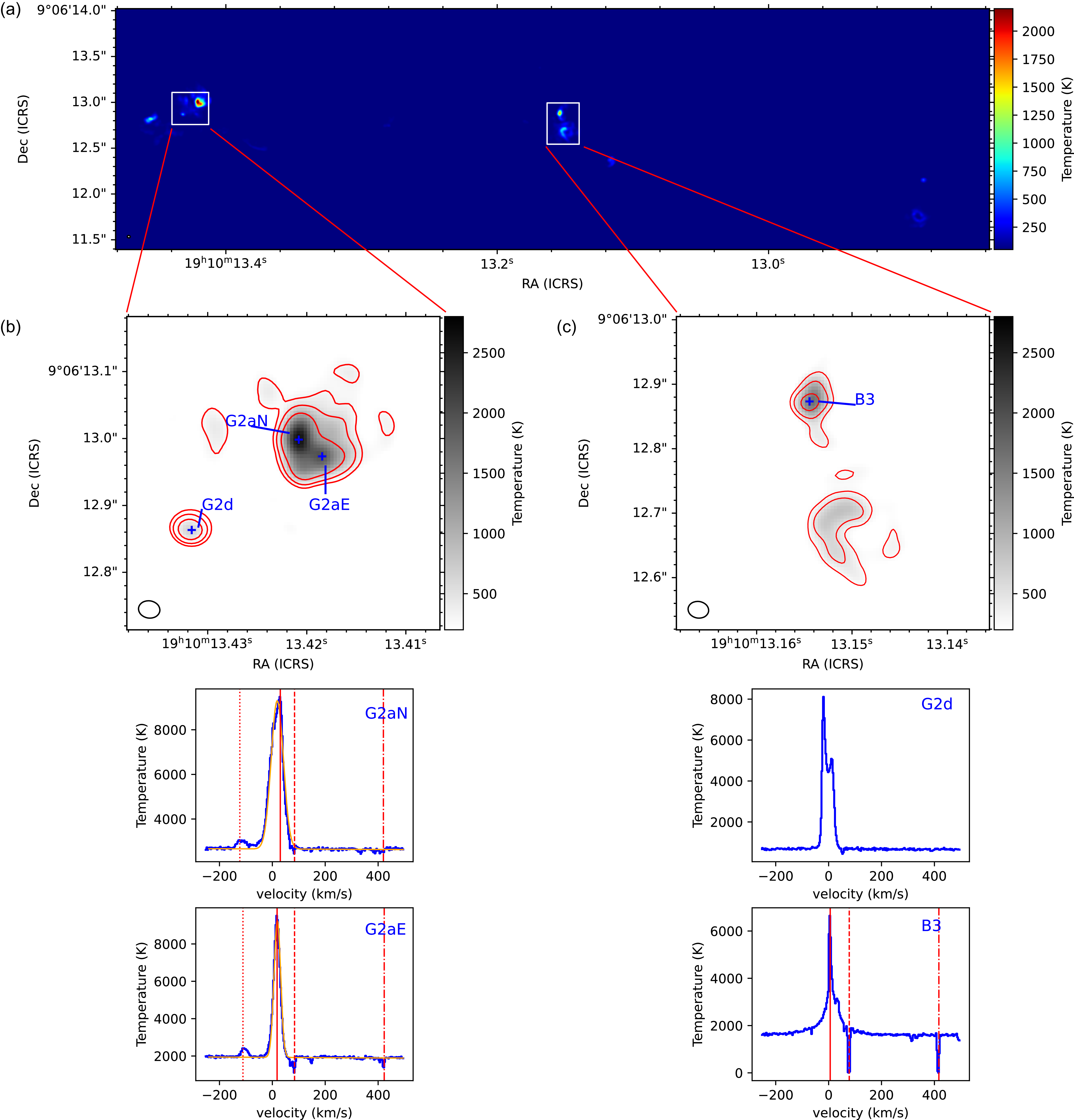
RRL maser candidate B3 was identified by its narrow line width. The top panel (a) of Figure 1 shows the spatial distribution of the 256 GHz continuum emission, with white boxes highlighting the regions where H29
$\alpha$
RRL maser candidate B3 was identified by its narrow line width. The top panel (a) of Figure 1 shows the spatial distribution of the 256 GHz continuum emission, with white boxes highlighting the regions where H29 $\alpha$
maser candidates are detected.
$\alpha$
maser candidates are detected.
Spatial distribution of regions with RRL maser emission and corresponding line profiles. Panel (a) shows the spatial distribution of the continuum, with white boxes indicating the regions exhibiting RRL maser emission. Panels (b) and (c) provide zoomed-in views of the regions marked by the white boxes in panel (a). The continuum brightness temperature (K) is shown in greyscale, while the velocity-integrated map (moment 0) is represented by red contours. The contour levels in panels (b) and (c) are set to 25 000, 50 000 and 110 000(K km/s). The position of the maximum moment 0 in each maser emission region is marked as blue ‘ + ’. The lower panels display the corresponding line profiles for each maser source. The profiles for sources G2aN and G2aE are fitted with single Gaussian profiles, shown by the orange curves. In each spectrum, the detected H29 $\alpha$
emission is marked with a red solid line, the detected He29
$\alpha$
emission is marked with a red solid line, the detected He29 $\alpha$
emission with a red dotted line, the absorption line of SO
$\alpha$
emission with a red dotted line, the absorption line of SO $_2$
(
$_2$
( $5_{3,3} \rightarrow 5_{2,4}$
) is marked with a red dashed line, and the absorption line of SO
$5_{3,3} \rightarrow 5_{2,4}$
) is marked with a red dashed line, and the absorption line of SO $_2$
(
$_2$
( $3_{3,1} \rightarrow 3_{2,2}$
) with a red dash-dotted line.
$3_{3,1} \rightarrow 3_{2,2}$
) with a red dash-dotted line.

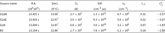
Parameters of central sources of W49A.
 $^{\mathrm{a}}$
The line optical depth at frequency
$^{\mathrm{a}}$
The line optical depth at frequency $\nu$
under non-LTE conditions.
$\nu$
under non-LTE conditions.
Panels (b) and (c) of Figure 1 present zoomed-in views of the regions enclosed by the white boxes in panel (a), showing the spatial distribution of the H29 $\alpha$
velocity-integrated intensity represented by red contours and the 256 GHz continuum emission shown in greyscale. The sources G2a and B3 are named following the 7mm continuum emission reported by De Pree et al. (Reference De Pree2018, Reference De Pree2020). G2a was first resolved into two distinct sources in our observation, named as G2aN (north) and G2aE (east), both of which exhibit features of maser emission. G2d, which was first identified in this region, is an HC H II region showing strong H29
$\alpha$
velocity-integrated intensity represented by red contours and the 256 GHz continuum emission shown in greyscale. The sources G2a and B3 are named following the 7mm continuum emission reported by De Pree et al. (Reference De Pree2018, Reference De Pree2020). G2a was first resolved into two distinct sources in our observation, named as G2aN (north) and G2aE (east), both of which exhibit features of maser emission. G2d, which was first identified in this region, is an HC H II region showing strong H29 $\alpha$
maser candidate features, although it is nearly unresolved in our observation. The velocity integration ranges for panels (b) and (c) were derived from spatially averaged spectra of the respective sources. In panel (b), the integration ranges are as follows:
$\alpha$
maser candidate features, although it is nearly unresolved in our observation. The velocity integration ranges for panels (b) and (c) were derived from spatially averaged spectra of the respective sources. In panel (b), the integration ranges are as follows: $-72$
to
$-72$
to $+71$
km/s for G2aN,
$+71$
km/s for G2aN, $-30$
to
$-30$
to $+65$
km/s for G2aE, and
$+65$
km/s for G2aE, and $-75$
to
$-75$
to $+70$
km/s for G2d. In panel (c), which corresponds to source B3, the range is
$+70$
km/s for G2d. In panel (c), which corresponds to source B3, the range is $-62$
to
$-62$
to $+60$
km/s. The peak positions of the H29
$+60$
km/s. The peak positions of the H29 $\alpha$
velocity-integrated emission in the four RRL maser candidate regions are marked by blue ‘ +’ in panels (b) and (c) of Figure 1. The detailed parameters for these positions, including their coordinates and free-free continuum at this frequency, are presented in Table 1.
$\alpha$
velocity-integrated emission in the four RRL maser candidate regions are marked by blue ‘ +’ in panels (b) and (c) of Figure 1. The detailed parameters for these positions, including their coordinates and free-free continuum at this frequency, are presented in Table 1.
The lower panels of Figure 1 show the corresponding line profiles at the peak positions. He29 $\alpha$
emission was detected towards G2aN and G2aE (see the line profiles in Figure 1), while it was not detected in the other two sources. Absorption lines of SO
$\alpha$
emission was detected towards G2aN and G2aE (see the line profiles in Figure 1), while it was not detected in the other two sources. Absorption lines of SO $_2$
(
$_2$
( $5_{3,3} \rightarrow 5_{2,4}$
) and SO
$5_{3,3} \rightarrow 5_{2,4}$
) and SO $_2$
(
$_2$
( $3_{3,1} \rightarrow 3_{2,2}$
) were observed towards all four sources, coincident with regions of strong free-free continuum emission, which is particularly pronounced towards B3. Both SO
$3_{3,1} \rightarrow 3_{2,2}$
) were observed towards all four sources, coincident with regions of strong free-free continuum emission, which is particularly pronounced towards B3. Both SO $_{2}$
absorption lines seem to be optically thick, with the absorption dips close to zero. The corresponding line profiles are shown in Figure 1, where the detected H29
$_{2}$
absorption lines seem to be optically thick, with the absorption dips close to zero. The corresponding line profiles are shown in Figure 1, where the detected H29 $\alpha$
emission, He29
$\alpha$
emission, He29 $\alpha$
emission, SO
$\alpha$
emission, SO $_2$
(
$_2$
( $5_{3,3} \rightarrow 5_{2,4}$
) absorption, and SO
$5_{3,3} \rightarrow 5_{2,4}$
) absorption, and SO $_2$
(
$_2$
( $3_{3,1} \rightarrow 3_{2,2}$
) absorption are represented by red solid, red dotted, red dashed, and red dash-dotted lines, respectively. The line profiles for G2aN and G2aE were fitted with a single Gaussian, represented by the orange curves.
$3_{3,1} \rightarrow 3_{2,2}$
) absorption are represented by red solid, red dotted, red dashed, and red dash-dotted lines, respectively. The line profiles for G2aN and G2aE were fitted with a single Gaussian, represented by the orange curves.
3.2 Identification of RRL maser candidates
3.2.1 G2aN and G2aE
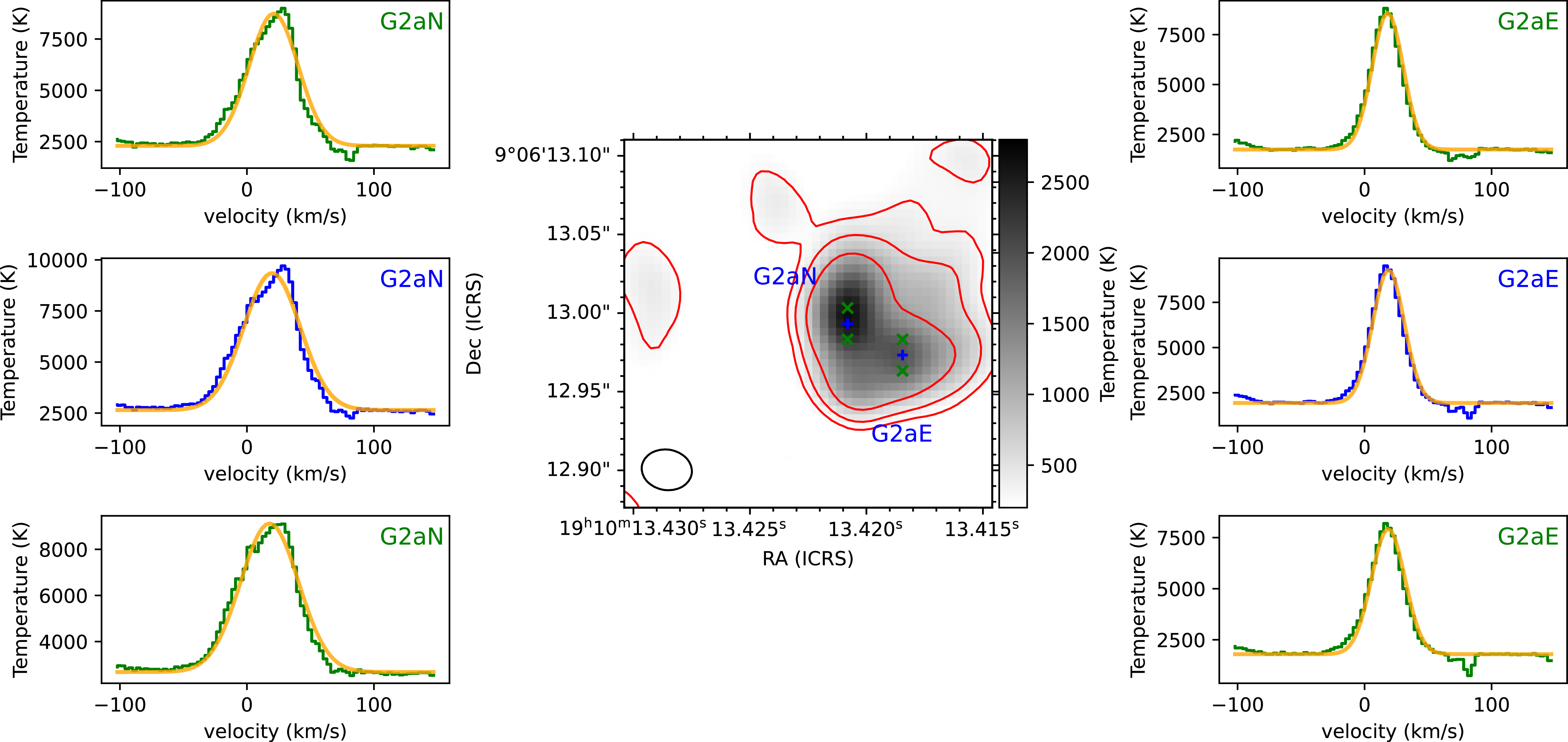
With a spatial resolution of $\sim0.03''$
, G2aN and G2aE are resolved as distinct sources, each exhibiting different line widths. The middle panel of Figure 2 provides zoomed-in views of Figure 1(b). Using the blue ‘+’ as a reference for each source, one point is selected above and one below along the minor axis of the beam, both marked with green ‘X’. The left and right panels show the line profiles corresponding to these positions, with the profiles arranged from top to bottom in the same order as their associated positions in the middle panel. (The same point-selection principle applies to Figures 3 and 4). The line profiles for both G2aN and G2aE were fitted with single-component Gaussians, overlaid with orange curves, and the relevant fitting parameters are listed in Table 2.
$\sim0.03''$
, G2aN and G2aE are resolved as distinct sources, each exhibiting different line widths. The middle panel of Figure 2 provides zoomed-in views of Figure 1(b). Using the blue ‘+’ as a reference for each source, one point is selected above and one below along the minor axis of the beam, both marked with green ‘X’. The left and right panels show the line profiles corresponding to these positions, with the profiles arranged from top to bottom in the same order as their associated positions in the middle panel. (The same point-selection principle applies to Figures 3 and 4). The line profiles for both G2aN and G2aE were fitted with single-component Gaussians, overlaid with orange curves, and the relevant fitting parameters are listed in Table 2.
Based on the parameters in Table 2, the median full width at half maximum (FWHM) is $51.4$
km s
$51.4$
km s $^{-1}$
for G2aN and
$^{-1}$
for G2aN and $29.2$
km s
$29.2$
km s $^{-1}$
for G2aE. High brightness temperatures, up to
$^{-1}$
for G2aE. High brightness temperatures, up to $\sim$
9 000 K, are observed in both G2aN and G2aE (see Figures 1 and 2), which may be explained as maser because the typical electron temperature of ionised gas, as the upper limit of brightness temperature of optically thick thermal emission, is about 8 000–10 000 K.
$\sim$
9 000 K, are observed in both G2aN and G2aE (see Figures 1 and 2), which may be explained as maser because the typical electron temperature of ionised gas, as the upper limit of brightness temperature of optically thick thermal emission, is about 8 000–10 000 K.
3.2.2 G2d
The H29 $\alpha$
spectrum towards the peak position of G2d exhibits a sharp feature that cannot be fitted with a Gaussian(see Figure 1), which is a typical signature of maser emission. A high brightness temperature reaching up to 8 000 K in G2d further supports the maser hypothesis. Despite the
$\alpha$
spectrum towards the peak position of G2d exhibits a sharp feature that cannot be fitted with a Gaussian(see Figure 1), which is a typical signature of maser emission. A high brightness temperature reaching up to 8 000 K in G2d further supports the maser hypothesis. Despite the $\sim$ $0.03''$
spatial resolution being insufficient to fully resolve G2d, the source size is unlikely to be significantly smaller than the beam size, given that markedly different line profiles are observed along the minor axis of the beam (see the spectra in Figure 3).
$0.03''$
spatial resolution being insufficient to fully resolve G2d, the source size is unlikely to be significantly smaller than the beam size, given that markedly different line profiles are observed along the minor axis of the beam (see the spectra in Figure 3).
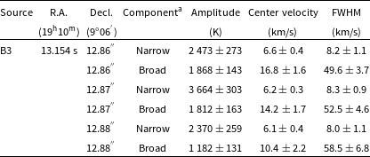
3.2.3 B3
Sharp line profiles are also observed in source B3, as shown in Figures 1 and 4. Both a narrow and another broad component can be found in the spectrum of source B3. By performing a two-component (narrow + broad) Gaussian fit to this spectrum (see Figure 4), we obtained the fitting parameters including the FWHMs of the narrow and broad components, as detailed in Table 3. The median FWHM of the narrow component is $8.2$
km s
$8.2$
km s $^{-1}$
,which is less than 10 km s
$^{-1}$
,which is less than 10 km s $^{-1}$
and can be explained by maser emission. This is because, for ionised gas near massive stars, the typical electron temperature is 8 000–10 000 K, the FWHM of thermal broadening of atomic hydrogen should be approximately 20 km s
$^{-1}$
and can be explained by maser emission. This is because, for ionised gas near massive stars, the typical electron temperature is 8 000–10 000 K, the FWHM of thermal broadening of atomic hydrogen should be approximately 20 km s $^{-1}$
.
$^{-1}$
.
Spatial distribution maps and corresponding spectral line profiles for sources G2aN and G2aE. Left panel: Spectral line profiles for source G2aN (top to bottom). Middle panel: A zoomed-in view of the spatial distribution of both sources at their corresponding positions, as indicated in Figure 1. Right panel: Spectral line profiles for source G2aE (top to bottom).

Left: A zoomed-in spatial distribution map of G2d with three beam minor-axis positions marked by blue ‘+’ and green ‘X’. Right: Corresponding spectral profiles (top to bottom) for these positions.

Left: A zoomed-in spatial distribution of B3, with three sampling positions along the minor axis of the beam marked by blue ‘+’ and green ‘X’. Right: Corresponding spectral line profiles for these positions (top to bottom), along with their double-Gaussian fitting curves. The red dash-dotted line represents the broad component, the green dashed line represents the narrow component, and the orange solid line represents the combined fit of both components (broad + narrow).

4. Discussion
4.1 The physical parameters of the RRL maser regions in W49A
The free-free continuum optical depth, $\tau_{\nu,C}$
, can be estimated from the measured continuum emission
$\tau_{\nu,C}$
, can be estimated from the measured continuum emission $T_{b}$
in units of K, with
$T_{b}$
in units of K, with
 \begin{equation}\tau_{\nu,C}=-\ln\left( 1-\frac{T_{b}}{T_{_{e}}} \right).\end{equation}
The calculated $\tau_{\nu,C}$
with electron temperature
$\tau_{\nu,C}$
with electron temperature $T_e=10\,000$
K in each source are listed in Table 1, with the maximum value of 0.31 towards G2aN. The emission measure (EM) is related to electron density (
$T_e=10\,000$
K in each source are listed in Table 1, with the maximum value of 0.31 towards G2aN. The emission measure (EM) is related to electron density ( $n_{e}$
) and the length along the line of sight (D), with EM=
$n_{e}$
) and the length along the line of sight (D), with EM= $n_{e}^{2}\times D$
. Based on Eq. (2.94) in Gordon & Sorochenko (Reference Gordon and Sorochenko2002) with the Rayleigh-Jeans approximation
$n_{e}^{2}\times D$
. Based on Eq. (2.94) in Gordon & Sorochenko (Reference Gordon and Sorochenko2002) with the Rayleigh-Jeans approximation $\left( h\,\nu \ll k\,T_{e} \right)$
, the free-free continuum absorption coefficient
$\left( h\,\nu \ll k\,T_{e} \right)$
, the free-free continuum absorption coefficient $\kappa_{C}$
as a function of frequency
$\kappa_{C}$
as a function of frequency $\nu$
can be evaluated numerically as
$\nu$
can be evaluated numerically as
 \begin{equation}\kappa_{\nu,C}=9.770\times 10^{-3}\frac{n_{e}n_{i}}{\nu^{2}T_{e}^{1.5}}\left[ 17.72+\ln\frac{T_{e}^{1.5}}{\nu} \right].\end{equation}
where $\kappa_{\nu,C}$
is expressed in units of
$\kappa_{\nu,C}$
is expressed in units of $\mathrm{cm}^{-1}$
,
$\mathrm{cm}^{-1}$
, $n_{e}$
in
$n_{e}$
in $\mathrm{cm}^{-3}$
,
$\mathrm{cm}^{-3}$
, $T_{e}$
in K, and
$T_{e}$
in K, and $\nu$
in Hz. Accordingly, the electron density
$\nu$
in Hz. Accordingly, the electron density $n_{e}$
can be written as:
$n_{e}$
can be written as:
 \begin{align}n_{e}^{2} = & -\ln\left[ 1 - \frac{T_{b}}{B_{\nu}(T_{e})} \right]\times \frac{\nu^{2}T_{e}^{1.5}}{17.72 + \ln\dfrac{T_{e}^{1.5}}{\nu}} \nonumber \\& \times 9.770^{-1} \times D^{-1} \times 10^{3}\end{align}
where $B_\nu(T_e)$
represents the Planck function at frequency
$B_\nu(T_e)$
represents the Planck function at frequency $\nu$
and temperature
$\nu$
and temperature $T_e$
.
$T_e$
.
As a rough estimation, spherical symmetry is assumed for each source exhibiting maser emission, with the source diameter taken to be comparable to the restoring beam size. The adopted value for diameter is 0.0032 pc, which is smaller than the maximum typical size of $0.03\ \mathrm{pc}$
for HC H II regions as reported by Kurtz (Reference Kurtz, Cesaroni, Felli, Churchwell and Walmsley2005), Keto et al. (Reference Keto, Zhang and Kurtz2008) and De Pree et al. (Reference De Pree2020). This approximation is reasonable, as the sources are only marginally resolved, while the electron density
$0.03\ \mathrm{pc}$
for HC H II regions as reported by Kurtz (Reference Kurtz, Cesaroni, Felli, Churchwell and Walmsley2005), Keto et al. (Reference Keto, Zhang and Kurtz2008) and De Pree et al. (Reference De Pree2020). This approximation is reasonable, as the sources are only marginally resolved, while the electron density $n_{\mathrm{e}}$
is
$n_{\mathrm{e}}$
is $\propto D^{-1/2}$
. The estimated values of
$\propto D^{-1/2}$
. The estimated values of $n_{e}$
for each source are presented in Table 1, in the level of several times of
$n_{e}$
for each source are presented in Table 1, in the level of several times of $10^{6}\,\mathrm{cm}^{-3}$
.
$10^{6}\,\mathrm{cm}^{-3}$
.
Amplification in RRL masers requires that the spectral-line optical depth be not only negative, indicating population inversion in the principal quantum levels, but also that its absolute value should be larger than the optical depth of free–free continuum, which is always positive (Gordon & Sorochenko Reference Gordon and Sorochenko2002). In non-LTE conditions, the line optical depth at frequency $\nu$
can be expressed as
$\nu$
can be expressed as $\tau_{\nu,L}^{\mathrm{nonLTE}} = \tau_{\nu,L}^{\mathrm{LTE}} \, b_{n_1} \, \beta_{n_1,n_2}$
, where
$\tau_{\nu,L}^{\mathrm{nonLTE}} = \tau_{\nu,L}^{\mathrm{LTE}} \, b_{n_1} \, \beta_{n_1,n_2}$
, where $\tau_{\nu,L}^{\mathrm{LTE}}$
is the corresponding LTE optical depth at frequency
$\tau_{\nu,L}^{\mathrm{LTE}}$
is the corresponding LTE optical depth at frequency $\nu$
, which can be obtained from Eq. (2.114) of Gordon & Sorochenko (Reference Gordon and Sorochenko2002). Both coefficients
$\nu$
, which can be obtained from Eq. (2.114) of Gordon & Sorochenko (Reference Gordon and Sorochenko2002). Both coefficients $b_{n_1}$
and
$b_{n_1}$
and $\beta_{n_1,n_2}$
are functions of the
$\beta_{n_1,n_2}$
are functions of the $T_e$
and
$T_e$
and $n_e$
(Zhu et al. Reference Zhu, Wang, Zhu and Zhang2022; Lu et al. Reference Lu2025).
$n_e$
(Zhu et al. Reference Zhu, Wang, Zhu and Zhang2022; Lu et al. Reference Lu2025).
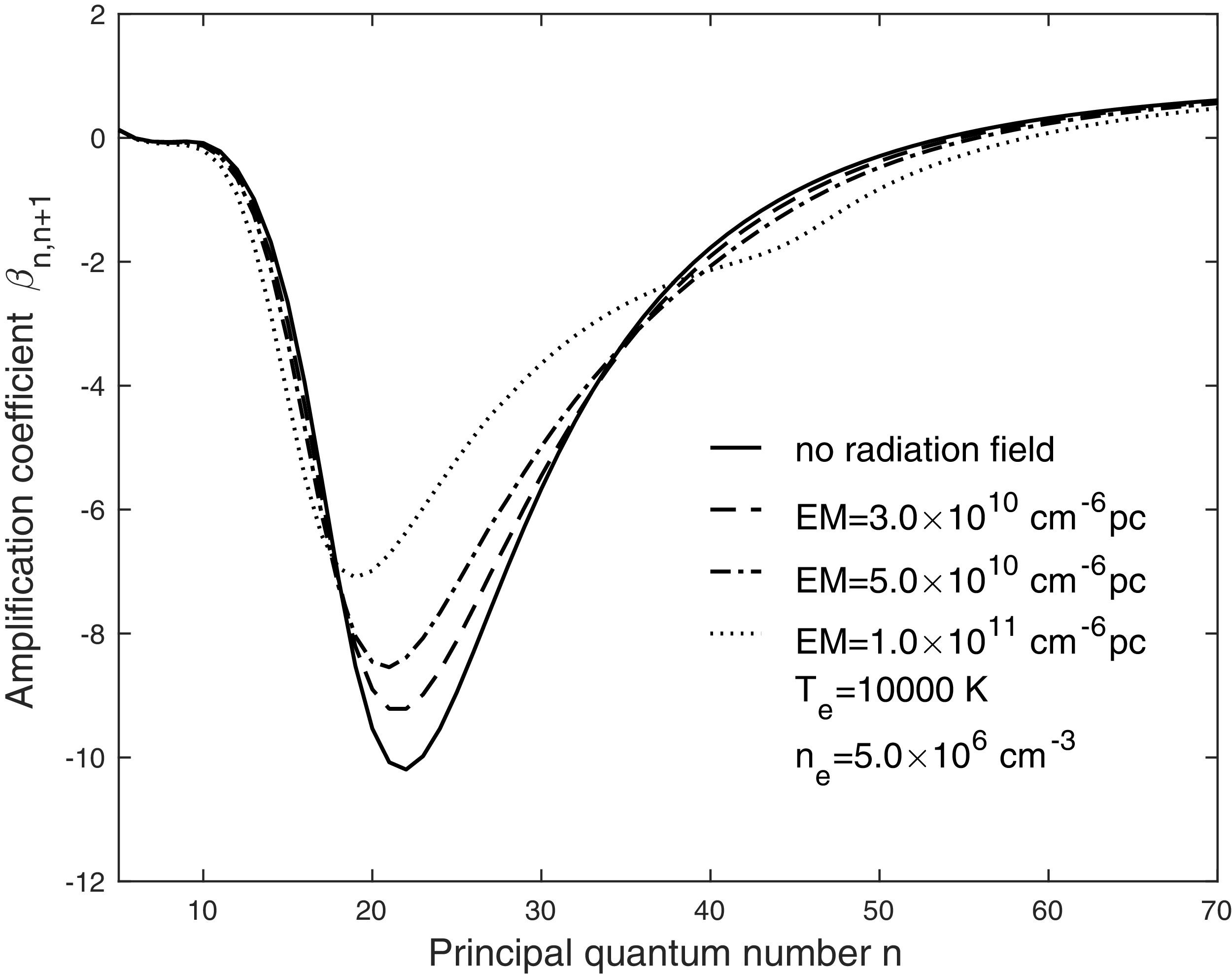
The amplification coefficients $\beta_{n,n+1}$
measure the deviation of the level population from LTE. The larger absolute value of
$\beta_{n,n+1}$
measure the deviation of the level population from LTE. The larger absolute value of $\beta_{n,n+1}$
, the stronger the maser amplification. For an electron density of
$\beta_{n,n+1}$
, the stronger the maser amplification. For an electron density of $5\times10^{6}\,\mathrm{cm}^{-3}$
, the most significant population inversion occurs for principal quantum numbers n between 20 and 25, depending on the EM, as shown in in Figure 5, calculated with the method from Zhu et al. (Reference Zhu, Wang, Zhu and Zhang2022). H29
$5\times10^{6}\,\mathrm{cm}^{-3}$
, the most significant population inversion occurs for principal quantum numbers n between 20 and 25, depending on the EM, as shown in in Figure 5, calculated with the method from Zhu et al. (Reference Zhu, Wang, Zhu and Zhang2022). H29 $\alpha$
is not located exactly at, but is close to, the most significantly inverted levels, which causes the detected masers. RRLs with the principal quantum numbers
$\alpha$
is not located exactly at, but is close to, the most significantly inverted levels, which causes the detected masers. RRLs with the principal quantum numbers $n\lt29$
at higher frequencies, may have more significant maser signatures towards these sources. Therefore, H26
$n\lt29$
at higher frequencies, may have more significant maser signatures towards these sources. Therefore, H26 $\alpha$
at 353.623 GHz, with both significant population inversion and good atmospheric transmission, is the best choice for discovering new RRLs masers with high-resolution ALMA observations.
$\alpha$
at 353.623 GHz, with both significant population inversion and good atmospheric transmission, is the best choice for discovering new RRLs masers with high-resolution ALMA observations.
The highest $n_e$
among these sources is approximately 6.7
$n_e$
among these sources is approximately 6.7 $\times10^6\,\mathrm{cm}^{-3}$
in G2aN, which results in less than 3% pressure broadening of the thermal broadening for H29
$\times10^6\,\mathrm{cm}^{-3}$
in G2aN, which results in less than 3% pressure broadening of the thermal broadening for H29 $\alpha$
, calculated with
$\alpha$
, calculated with $\frac{\Delta \nu_{L}}{\Delta \nu_{t}}=1.2\left( \frac{n_{e}}{10^{5}} \right)\left( \frac{n}{92} \right)^{7}$
(Keto et al. Reference Keto, Zhang and Kurtz2008), where
$\frac{\Delta \nu_{L}}{\Delta \nu_{t}}=1.2\left( \frac{n_{e}}{10^{5}} \right)\left( \frac{n}{92} \right)^{7}$
(Keto et al. Reference Keto, Zhang and Kurtz2008), where $\Delta \nu_{L}$
is for pressure broadening,
$\Delta \nu_{L}$
is for pressure broadening, $\Delta \nu_{t}$
is for the thermal width, and n is the principal quantum number. Thus, pressure broadening can be neglected for all these RRL maser sources. The dominant broadening mechanisms should be thermal motion and turbulence. The FWHM caused by thermal broadening of hydrogen atomics at 10 000 K is 21.4 km s
$\Delta \nu_{t}$
is for the thermal width, and n is the principal quantum number. Thus, pressure broadening can be neglected for all these RRL maser sources. The dominant broadening mechanisms should be thermal motion and turbulence. The FWHM caused by thermal broadening of hydrogen atomics at 10 000 K is 21.4 km s $^{-1}$
(De Pree et al. Reference De Pree2004), while it is about 51 km s
$^{-1}$
(De Pree et al. Reference De Pree2004), while it is about 51 km s $^{-1}$
in G2aN and 29 km s
$^{-1}$
in G2aN and 29 km s $^{-1}$
in G2aE for H29
$^{-1}$
in G2aE for H29 $\alpha$
(see spectra in Figures 1 and 2, fitting parameters in Table 2), which can not be explained without turbulence. The optical depths of H29
$\alpha$
(see spectra in Figures 1 and 2, fitting parameters in Table 2), which can not be explained without turbulence. The optical depths of H29 $\alpha$
at the positions of peak velocity-integrated in these four sources range from
$\alpha$
at the positions of peak velocity-integrated in these four sources range from $-1.8$
to
$-1.8$
to $-3.4$
, as calculated from the measured line and continuum data using the methods described by Zhu et al. (Reference Zhu, Wang, Zhu and Zhang2022) and Lu et al. (Reference Lu2025). These values are consistent with observational signatures of maser candidates.
$-3.4$
, as calculated from the measured line and continuum data using the methods described by Zhu et al. (Reference Zhu, Wang, Zhu and Zhang2022) and Lu et al. (Reference Lu2025). These values are consistent with observational signatures of maser candidates.
Spectral line parameters for sources G2aN and G2aE from single-Gaussian fitting.
 $^{\mathrm{a}}$
Peak intensity of the Gaussian fit to the spectral line profile.
$^{\mathrm{a}}$
Peak intensity of the Gaussian fit to the spectral line profile. $^{\mathrm{b}}$
Velocity at the centre of the Gaussian fit to the spectral line profile.
$^{\mathrm{b}}$
Velocity at the centre of the Gaussian fit to the spectral line profile. $^{\mathrm{c}}$
Full width at half maximum of the Gaussian fit to the spectral line profile.
$^{\mathrm{c}}$
Full width at half maximum of the Gaussian fit to the spectral line profile.
These parameters have the same meanings as those in Table 3.
Parameters of the double-Gaussian (broad and narrow) component fitting for the spectral line profile of source B3.
 $^{\mathrm{a}}$
The ‘Broad’ and ‘Narrow’ components refer to the two Gaussian components used in the fitting of the spectral line profile.
$^{\mathrm{a}}$
The ‘Broad’ and ‘Narrow’ components refer to the two Gaussian components used in the fitting of the spectral line profile.
Since G2d, where sharp features of H29 $\alpha$
were detected, was only marginally resolved, the brightness temperatures of both line and continuum were underestimated, which can cause the underestimation of EM,
$\alpha$
were detected, was only marginally resolved, the brightness temperatures of both line and continuum were underestimated, which can cause the underestimation of EM, $n_e$
, as well as the absolute value of opacities of free-free continuum and H29
$n_e$
, as well as the absolute value of opacities of free-free continuum and H29 $\alpha$
.
$\alpha$
.
The amplification coefficients $\beta_{n,n+1}$
for
$\beta_{n,n+1}$
for $T_{e}=10\,000$
K and
$T_{e}=10\,000$
K and $n_{e} = 5.0\times10^{6}\,\mathrm{cm}^{-3}$
in an H II region with different EMs.
$n_{e} = 5.0\times10^{6}\,\mathrm{cm}^{-3}$
in an H II region with different EMs.

4.2 How to find RRL masers efficiently
Extremely high brightness temperature, narrow line width, and/or sharp line profile are the most distinguishing features for identifying maser candidates from the spectroscopic observations. The spatial distribution of the peak temperature, as shown in Figure 6, can be used to identify potential RRL maser candidates. With their high peak brightness temperatures, sources G2aN and G2aE can be easily identified as maser candidates, while G2d and B3 may be overlooked using this criterion.
The spatial distribution of the peak temperature (K), with positions exhibiting peak values lower than 2 000 K being excluded.

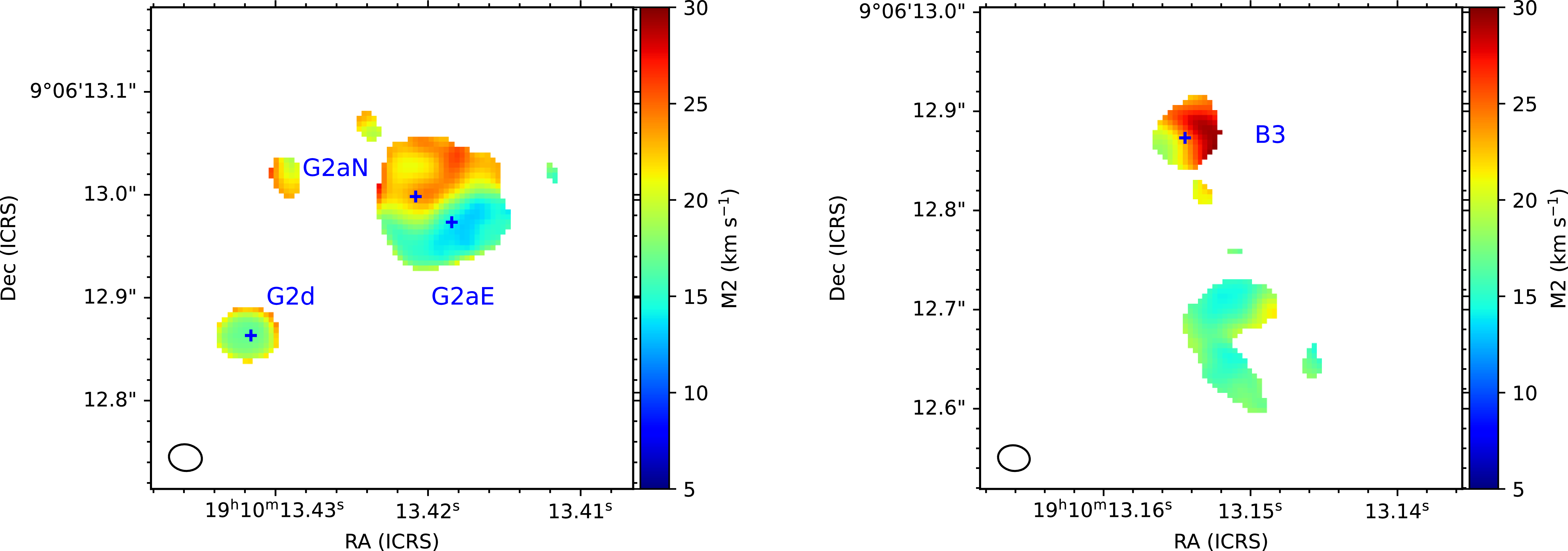
The second moment (see Figure 7), weighted by intensity, describes the dispersion of the spectrum relative to the centroid velocity ${v_0}$
. For a Gaussian spectrum, the second moment approximates the velocity dispersion,
${v_0}$
. For a Gaussian spectrum, the second moment approximates the velocity dispersion, $\sigma_{v}$
, which is related to the FWHM as
$\sigma_{v}$
, which is related to the FWHM as $\sqrt{8\ln 2} \sigma_v \approx 2.35 \, \sigma_v$
. Spectral lines in regions where the masers occur should exhibit relatively narrow line widths due to exponential amplification. In typical ionised gas regions with an electron temperature of 10 000 K, the corresponding velocity dispersion is about
$\sqrt{8\ln 2} \sigma_v \approx 2.35 \, \sigma_v$
. Spectral lines in regions where the masers occur should exhibit relatively narrow line widths due to exponential amplification. In typical ionised gas regions with an electron temperature of 10 000 K, the corresponding velocity dispersion is about $9.1\,\mathrm{km\,s^{-1}}$
, or about
$9.1\,\mathrm{km\,s^{-1}}$
, or about $21.4\,\mathrm{km\,s^{-1}}$
for FWHM. However, such low values are below
$21.4\,\mathrm{km\,s^{-1}}$
for FWHM. However, such low values are below $10\,\mathrm{km\,s^{-1}}$
, are not observed in the second moment map (see Figure 7), which is mainly because a broad component often exists, as can be seen in the line profiles of source B3, as illustrated in Figures 1 and 4. Thus, the second moment map is not efficient for searching RRL maser candidates.
$10\,\mathrm{km\,s^{-1}}$
, are not observed in the second moment map (see Figure 7), which is mainly because a broad component often exists, as can be seen in the line profiles of source B3, as illustrated in Figures 1 and 4. Thus, the second moment map is not efficient for searching RRL maser candidates.
The spatial distribution of the second moment in ionised gas regions with a typical electron temperature of $10\,000$
K.
$10\,000$
K.

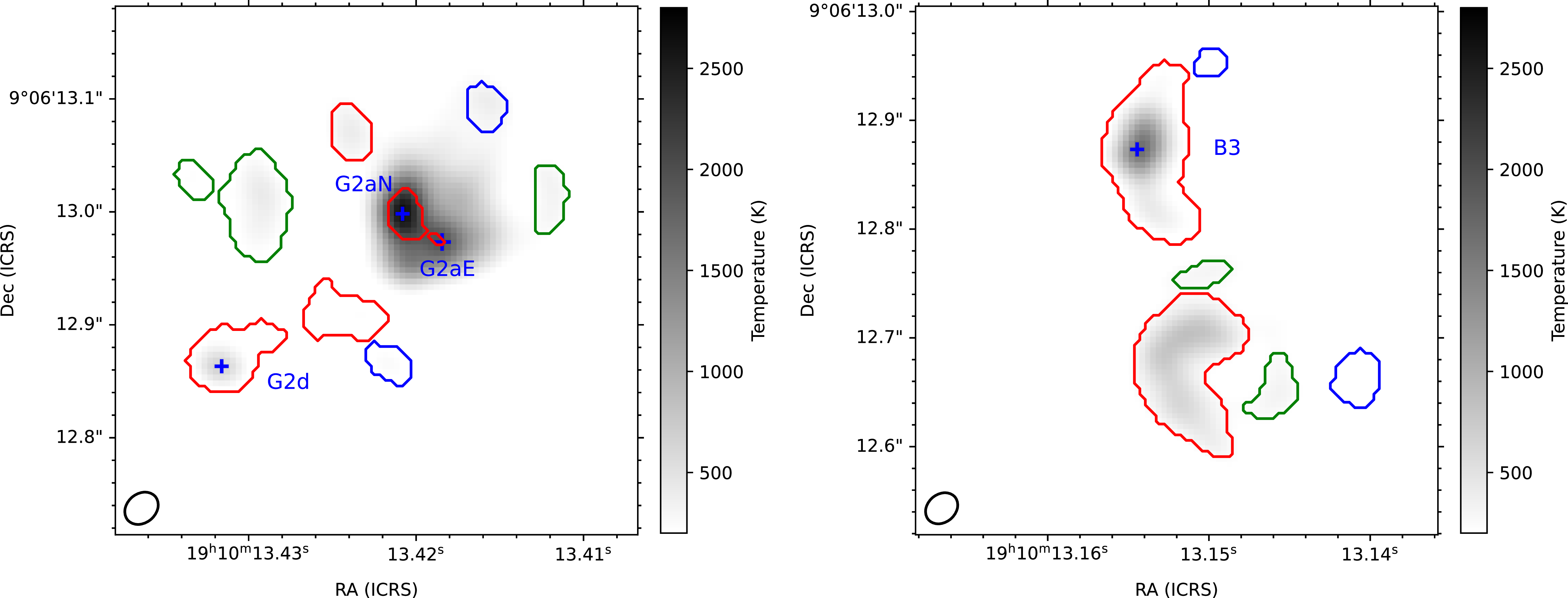
The observed line-to-continuum ratio between velocity integrated RRL and free-free emission can be used to determine population inversion (Gordon & Sorochenko Reference Gordon and Sorochenko2002; Zhu et al. Reference Zhu, Wang, Zhu and Zhang2022; Lu et al. Reference Lu2025). This ratio can therefore be useful for selecting RRL maser candidates. We applied the dendrogram technique (Rosolowsky et al. Reference Rosolowsky, Pineda, Kauffmann and Goodman2008) to continuum images obtained from line-free channels to identify sources. Regions with a signal-to-noise ratio (SNR) below 5 were excluded, and structures with peak values exceeding 10 times the noise standard deviation (10 $\sigma$
) were considered independent. With the requirement of minimum number of pixels equal to the synthesised beam, 24 sources were identified in this region, and their parameters are listed in Table A1. Among the 24 sources, 16 are located in two small areas (see the middle panels of Figure 1, 6–8). Since the line-to-continuum ratios vary pixel by pixel, the maximal line-to-continuum ratio within each source was used for classification, as shown in Figure 8. 12 out of 24 sources, including 4 sources exhibiting maser emission, have a maximal line-to-continuum ratio within each source greater than
$\sigma$
) were considered independent. With the requirement of minimum number of pixels equal to the synthesised beam, 24 sources were identified in this region, and their parameters are listed in Table A1. Among the 24 sources, 16 are located in two small areas (see the middle panels of Figure 1, 6–8). Since the line-to-continuum ratios vary pixel by pixel, the maximal line-to-continuum ratio within each source was used for classification, as shown in Figure 8. 12 out of 24 sources, including 4 sources exhibiting maser emission, have a maximal line-to-continuum ratio within each source greater than $\sim$
110 km s
$\sim$
110 km s $^{-1}$
. If a threshold of
$^{-1}$
. If a threshold of $\sim$
90 km s
$\sim$
90 km s $^{-1}$
is used, the number of sources increases to 19 out of 24. Notably, the maximal line-to-continuum ratios for all 4 sources with maser sources exceed 120 km s
$^{-1}$
is used, the number of sources increases to 19 out of 24. Notably, the maximal line-to-continuum ratios for all 4 sources with maser sources exceed 120 km s $^{-1}$
. Thus, a maximal line-to-continuum ratio of 110 km s
$^{-1}$
. Thus, a maximal line-to-continuum ratio of 110 km s $^{-1}$
can serve as an effective criterion for identifying maser emission regions.
$^{-1}$
can serve as an effective criterion for identifying maser emission regions.
The spatial distribution of the ratio (km s $^{-1})$
between the moment 0 of the observed RRLs and the continuum at the corresponding frequency. The greyscale image represents the continuum, with the blue, green, and red contour lines indicating sources detected by the continuum. The different colours correspond to different ranges of the maximum line-to-continuum ratio: blue for
$^{-1})$
between the moment 0 of the observed RRLs and the continuum at the corresponding frequency. The greyscale image represents the continuum, with the blue, green, and red contour lines indicating sources detected by the continuum. The different colours correspond to different ranges of the maximum line-to-continuum ratio: blue for $\lt 90$
, green for
$\lt 90$
, green for $90 - 110$
, and red for
$90 - 110$
, and red for $\gt 110$
.
$\gt 110$
.

5. Summary
Using high resolution ( $\sim0.03''$
) of the H29
$\sim0.03''$
) of the H29 $\alpha$
observations from ALMA towards the Galactic massive star-forming region W49A, we have identified four new RRL maser candidates, based on sharp line profiles and/or high brightness temperatures. One source (G2d) was identified as RRL maser candidate, exhibiting both a sharp line profile and a high brightness temperature. The other two sources (G2aN and G2aE) were characterised by high brightness temperatures, while the last one (B3) was identified solely by its sharp line profile. Line opacities of these RRL maser candidates were also calculated to be around
$\alpha$
observations from ALMA towards the Galactic massive star-forming region W49A, we have identified four new RRL maser candidates, based on sharp line profiles and/or high brightness temperatures. One source (G2d) was identified as RRL maser candidate, exhibiting both a sharp line profile and a high brightness temperature. The other two sources (G2aN and G2aE) were characterised by high brightness temperatures, while the last one (B3) was identified solely by its sharp line profile. Line opacities of these RRL maser candidates were also calculated to be around $-2.5$
, which proves that they are RRL maser candidates. Searching for RRL maser candidates in regions with high peak temperature and high line-to-continuum ratio may improve efficiency. Future prospects of searching for new RRL maser candidates are also presented.
$-2.5$
, which proves that they are RRL maser candidates. Searching for RRL maser candidates in regions with high peak temperature and high line-to-continuum ratio may improve efficiency. Future prospects of searching for new RRL maser candidates are also presented.
Acknowledgements
This work is supported by National Key R&D Program of China (2023YFA1608204), the National Natural Science Foundation of China grant 12173067, and the Guangxi Talent Programme (Highland of Innovation Talents).
This paper makes use of the following ALMA data: ADS/JAO.ALMA 2018.1.00520.S. ALMA is a partnership of ESO (representing its member states), NSF (USA), and NINS (Japan), together with NRC (Canada), NSTC and ASIAA (Taiwan), and KASI (Republic of Korea), in cooperation with the Republic of Chile. The Joint ALMA Observatory is operated by ESO, AUI/NRAO, and NAOJ.
Data availability statement
The paper using data from ALMA archive system at https://almascience.nao.ac.jp/aq/ with the project number of 2018.1.00520.S. If anyone is interested in the reduced data presented in this paper, please contact Junzhi Wang at junzhiwang@gxu.edu.cn.
Appendix A. Continuum source parameters
We identified 24 continuum sources using the dendrogram technique. Their parameters are listed in Table A1.
Parameters of sources detected from the continuum.
 $^{\mathrm{a}}$
Peak continuum intensity for each source identified using the dendrogram technique.
$^{\mathrm{a}}$
Peak continuum intensity for each source identified using the dendrogram technique. $^{\mathrm{b}}$
Peak line-to-continuum ratio for each source identified using the dendrogram technique.
$^{\mathrm{b}}$
Peak line-to-continuum ratio for each source identified using the dendrogram technique.


 Open access