

1 Introduction
1.1 BZSV duality
In [Reference Ben-Zvi, Sakellaridis and Venkatesh1], Ben-Zvi, Sakellaridis, and Venkatesh introduced a striking relative Langlands duality for the so-called anomaly-free hyperspherical Hamiltonian spaces, which we will refer to as the BZSV duality. We begin by briefly recalling the key data involved.
Throughout this paper, k is a global field, ${\mathbb A}={\mathbb A}_k$
, F is a local field, and
${\mathbb A}={\mathbb A}_k$
, F is a local field, and $\psi $
is a nontrivial additive character of
$\psi $
is a nontrivial additive character of ${\mathbb A}/k$
(resp. F) if we are in the global (resp. local) setting. Let G be a split connected reductive group defined over k. In Section 3.5.1 of [Reference Ben-Zvi, Sakellaridis and Venkatesh1], Ben-Zvi, Sakellaridis, and Venkatesh defined a special category of G-Hamiltonian spaces called the hyperspherical G-Hamiltonian spaces. The most important condition for hyperspherical is the coisotropic condition (Condition (2) in Section 3.5.1 of [Reference Ben-Zvi, Sakellaridis and Venkatesh1]), which states that the field of G-invariant rational functions on the Hamiltonian space is commutative with respect to the Poisson bracket. In Theorem 3.6.1 of [Reference Ben-Zvi, Sakellaridis and Venkatesh1], Ben-Zvi, Sakellaridis, and Venkatesh proved a structure theorem stating that each hyperspherical G-Hamiltonian space is associated with a quadruple
${\mathbb A}/k$
(resp. F) if we are in the global (resp. local) setting. Let G be a split connected reductive group defined over k. In Section 3.5.1 of [Reference Ben-Zvi, Sakellaridis and Venkatesh1], Ben-Zvi, Sakellaridis, and Venkatesh defined a special category of G-Hamiltonian spaces called the hyperspherical G-Hamiltonian spaces. The most important condition for hyperspherical is the coisotropic condition (Condition (2) in Section 3.5.1 of [Reference Ben-Zvi, Sakellaridis and Venkatesh1]), which states that the field of G-invariant rational functions on the Hamiltonian space is commutative with respect to the Poisson bracket. In Theorem 3.6.1 of [Reference Ben-Zvi, Sakellaridis and Venkatesh1], Ben-Zvi, Sakellaridis, and Venkatesh proved a structure theorem stating that each hyperspherical G-Hamiltonian space is associated with a quadruple $\Delta =(G,H,\rho _H,\iota )$
where H is a split reductive subgroup of G;
$\Delta =(G,H,\rho _H,\iota )$
where H is a split reductive subgroup of G; $\rho _H$
is a symplectic representation of H; and
$\rho _H$
is a symplectic representation of H; and $\iota $
is a homomorphism from
$\iota $
is a homomorphism from ${\mathrm {SL}}_2$
into G whose image commutes with H. We will call such a quadruple the BZSV quadruple in this paper.
${\mathrm {SL}}_2$
into G whose image commutes with H. We will call such a quadruple the BZSV quadruple in this paper.
Let us briefly recall how to associate a G-Hamiltonian space ${\mathcal {M}}_{\Delta }$
to a BZSV quadruple
${\mathcal {M}}_{\Delta }$
to a BZSV quadruple $\Delta =(G,H,\rho _H,\iota )$
. Set
$\Delta =(G,H,\rho _H,\iota )$
. Set $\hbar (t):=\iota (\begin {pmatrix}t&0\\ 0&t^{-1}\end {pmatrix})$
in G and denote by L the centralizer of
$\hbar (t):=\iota (\begin {pmatrix}t&0\\ 0&t^{-1}\end {pmatrix})$
in G and denote by L the centralizer of $\hbar (t)$
and by
$\hbar (t)$
and by $U=\exp (\mathfrak u)$
(resp.
$U=\exp (\mathfrak u)$
(resp. $\bar {U}=\exp (\bar {\mathfrak u})$
) the corresponding unipotent subgroups of G associated with
$\bar {U}=\exp (\bar {\mathfrak u})$
) the corresponding unipotent subgroups of G associated with $\iota $
, where
$\iota $
, where $\mathfrak u\subset {\mathfrak {g}}$
(resp.
$\mathfrak u\subset {\mathfrak {g}}$
(resp. $\bar {\mathfrak u}\subset {\mathfrak {g}}$
) is the positive weight space (resp. negative weight space) of the Lie algebra
$\bar {\mathfrak u}\subset {\mathfrak {g}}$
) is the positive weight space (resp. negative weight space) of the Lie algebra ${\mathfrak {g}}$
of G under the adjoint action of
${\mathfrak {g}}$
of G under the adjoint action of $\hbar (t)$
. Then
$\hbar (t)$
. Then $P=LU$
and
$P=LU$
and $\bar {P}=L\bar {U}$
are parabolic subgroups of G that are opposite to each other. It is clear that
$\bar {P}=L\bar {U}$
are parabolic subgroups of G that are opposite to each other. It is clear that $H\subset L$
.
$H\subset L$
.
Let $\mathfrak u^+$
be the
$\mathfrak u^+$
be the $\geq 2$
weight space under the adjoint action of
$\geq 2$
weight space under the adjoint action of $\hbar (t)$
. It is well known that the vector space
$\hbar (t)$
. It is well known that the vector space $\mathfrak u/\mathfrak u^+$
has a symplectic structure and realizes a symplectic representation of H (and of L) under the adjoint action. If we use
$\mathfrak u/\mathfrak u^+$
has a symplectic structure and realizes a symplectic representation of H (and of L) under the adjoint action. If we use $V=V_{\rho _H}$
to denote the underlying vector space of the symplectic representation
$V=V_{\rho _H}$
to denote the underlying vector space of the symplectic representation $\rho _H$
, then the Hamiltonian variety
$\rho _H$
, then the Hamiltonian variety ${\mathcal {M}}_\Delta $
is defined to be ((3.17) of [Reference Ben-Zvi, Sakellaridis and Venkatesh1])
${\mathcal {M}}_\Delta $
is defined to be ((3.17) of [Reference Ben-Zvi, Sakellaridis and Venkatesh1])
 $$ \begin{align} {\mathcal {M}}_\Delta=((V\times \mathfrak{u}/\mathfrak{u}^+)\times _{({\mathfrak {h}}+\mathfrak{u})^\ast} {\mathfrak {g}}^\ast)\times ^{HU}G \end{align} $$
where
-
• the maps $\mathfrak {u}/\mathfrak {u}^+\rightarrow {\mathfrak {h}}^\ast $
and
$V\rightarrow {\mathfrak {h}}^\ast $
are the moment maps;
$\mathfrak {u}/\mathfrak {u}^+\rightarrow {\mathfrak {h}}^\ast $
and
$V\rightarrow {\mathfrak {h}}^\ast $
are the moment maps; -
• the map
$V\rightarrow \mathfrak {u}^\ast $
is the zero map; -
• the map
$\mu :\mathfrak {u}/\mathfrak {u}^+\rightarrow \mathfrak {u}^\ast $
is given by
$$ \begin{align*}\mu(u)=\kappa_1(u)+\kappa_f\end{align*} $$
where
$\kappa _1: \mathfrak {u}/\mathfrak {u}^+\rightarrow (\mathfrak {u}/\mathfrak {u}^+)^\ast $
is the isomorphism via the symplectic form on
$\mathfrak {u}/\mathfrak {u}^+$
and
$$ \begin{align*}\kappa_f(X)=(f,X),\;X\in \mathfrak{u},\;f=\iota\left(\begin{pmatrix} 0&0\\1&0\end{pmatrix}\right).\end{align*} $$


Theorem 3.6.1 of [Reference Ben-Zvi, Sakellaridis and Venkatesh1] states that any hyperspherical G-Hamiltonian space is of the form ${\mathcal {M}}_\Delta $
for some BZSV quadruple
${\mathcal {M}}_\Delta $
for some BZSV quadruple $\Delta =(G,H,\rho _H,\iota )$
.
$\Delta =(G,H,\rho _H,\iota )$
.
Remark 1.1. When $\Delta =(G,H,0,1)$
(here
$\Delta =(G,H,0,1)$
(here $1$
means the
$1$
means the ${\mathrm {SL}}_2$
-homomorphism is the trivial map and
${\mathrm {SL}}_2$
-homomorphism is the trivial map and $0$
means that the symplectic representation is zero dimensional), the Hamiltonian space
$0$
means that the symplectic representation is zero dimensional), the Hamiltonian space ${\mathcal {M}}_{\Delta }$
is just the cotangent bundle
${\mathcal {M}}_{\Delta }$
is just the cotangent bundle $T^\ast (G/H)$
for the variety
$T^\ast (G/H)$
for the variety $G/H$
. This is called the spherical variety case. When
$G/H$
. This is called the spherical variety case. When $\Delta =(G,G,\rho ,1)$
(which is the case we consider in this paper), the Hamiltonian space
$\Delta =(G,G,\rho ,1)$
(which is the case we consider in this paper), the Hamiltonian space ${\mathcal {M}}_{\Delta }$
is just the underlying vector space of the symplectic representation
${\mathcal {M}}_{\Delta }$
is just the underlying vector space of the symplectic representation $\rho $
. This is called the symplectic vector space case.
$\rho $
. This is called the symplectic vector space case.
Definition 1.2. We say that a quadruple $\Delta =(G,H,\rho _H,\iota )$
is hyperspherical if the associated Hamiltonian variety
$\Delta =(G,H,\rho _H,\iota )$
is hyperspherical if the associated Hamiltonian variety ${\mathcal {M}}_\Delta $
is.
${\mathcal {M}}_\Delta $
is.
Remark 1.3. As we explained above, the most important condition in the definition of hyperspherical is the coisotropic condition. By Proposition 3.6.3 of [Reference Ben-Zvi, Sakellaridis and Venkatesh1], the Hamiltonian space ${\mathcal {M}}_\Delta $
associated to a BZSV quadruple
${\mathcal {M}}_\Delta $
associated to a BZSV quadruple $\Delta =(G,H,\rho _H,\iota )$
is coisotropic if
$\Delta =(G,H,\rho _H,\iota )$
is coisotropic if $HU$
is a spherical subgroup in G (i.e. it acts with an open orbit in the flag variety of G) and the vector space
$HU$
is a spherical subgroup in G (i.e. it acts with an open orbit in the flag variety of G) and the vector space $V\times \mathfrak u/\mathfrak u^+$
is a coisotropic/multiplicity free symplectic representation of the generic stabilizer of G on the cotangent bundle
$V\times \mathfrak u/\mathfrak u^+$
is a coisotropic/multiplicity free symplectic representation of the generic stabilizer of G on the cotangent bundle $T^\ast (G/HU)$
or equivalently, the generic stabilizer of H on the cotangent bundle
$T^\ast (G/HU)$
or equivalently, the generic stabilizer of H on the cotangent bundle $T^\ast (L/H)$
(we say a symplectic representation is coisotropic, or multiplicity free if the field of invariant rational functions on the vector space is commutative with respect to the Poisson bracket). All multiplicity-free symplectic representations are completely classified by Knop [Reference Knop30] and Losev [Reference Losev35].
$T^\ast (L/H)$
(we say a symplectic representation is coisotropic, or multiplicity free if the field of invariant rational functions on the vector space is commutative with respect to the Poisson bracket). All multiplicity-free symplectic representations are completely classified by Knop [Reference Knop30] and Losev [Reference Losev35].
Next we explain the anomaly-free condition for a Hamiltonian space. Let $\Delta =(G,H,\rho _H,\iota )$
be a hyperspherical BZSV quadruple, and let
$\Delta =(G,H,\rho _H,\iota )$
be a hyperspherical BZSV quadruple, and let ${\mathcal {M}}_{\Delta }$
be the associated hyperspherical Hamiltonian space. The map
${\mathcal {M}}_{\Delta }$
be the associated hyperspherical Hamiltonian space. The map $\iota $
induces an adjoint action of
$\iota $
induces an adjoint action of $H\times {\mathrm {SL}}_2$
on the Lie algebra
$H\times {\mathrm {SL}}_2$
on the Lie algebra ${\mathfrak {g}}$
of G and we can decompose it as
${\mathfrak {g}}$
of G and we can decompose it as
 $$ \begin{align*}\oplus_{k\in I} \rho_k\otimes Sym^k\end{align*} $$
where $\rho _k$
is some representation of H and I is a finite subset of
$\rho _k$
is some representation of H and I is a finite subset of ${\mathbb {Z}}_{\geq 0}$
. We let
${\mathbb {Z}}_{\geq 0}$
. We let $I_{odd}$
be the subset of I containing all the odd numbers and we define
$I_{odd}$
be the subset of I containing all the odd numbers and we define
 $$ \begin{align} \rho_{H,\iota}=\rho_H\oplus (\oplus_{i\in I_{odd}} \rho_i). \end{align} $$
This is a symplectic representation of H.
Definition 1.4 (Proposition 5.1.2 of [Reference Ben-Zvi, Sakellaridis and Venkatesh1]).
We say that the Hamiltonian space ${\mathcal {M}}_{\Delta }$
is anomaly-free (or equivalently, the quadruple
${\mathcal {M}}_{\Delta }$
is anomaly-free (or equivalently, the quadruple $\Delta $
is anomaly-free) if the representation
$\Delta $
is anomaly-free) if the representation $\rho _{H,\iota }$
is a symplectic anomaly-free representation (see Definition 2.7) of H.
$\rho _{H,\iota }$
is a symplectic anomaly-free representation (see Definition 2.7) of H.
Let $\hat {G}$
be the dual group of G. The BZSV duality is a conjectural duality between the set of anomaly-free hyperspherical G-Hamiltonian spaces and the set of anomaly-free hyperspherical
$\hat {G}$
be the dual group of G. The BZSV duality is a conjectural duality between the set of anomaly-free hyperspherical G-Hamiltonian spaces and the set of anomaly-free hyperspherical $\hat {G}$
-Hamiltonian spaces, or equivalently, a conjectural duality between the set of anomaly-free hyperspherical BZSV quadruples of G and the set of anomaly-free hyperspherical BZSV quadruples of
$\hat {G}$
-Hamiltonian spaces, or equivalently, a conjectural duality between the set of anomaly-free hyperspherical BZSV quadruples of G and the set of anomaly-free hyperspherical BZSV quadruples of $\hat {G}$
. This proposed duality not only extends the classical Langlands program to a broader geometric setting but also provides a new perspective on the interaction between Hamiltonian symmetries and representation theory.
$\hat {G}$
. This proposed duality not only extends the classical Langlands program to a broader geometric setting but also provides a new perspective on the interaction between Hamiltonian symmetries and representation theory.
In [Reference Ben-Zvi, Sakellaridis and Venkatesh1], Ben-Zvi, Sakellaridis, and Venkatesh formulated a series of elegant and far-reaching conjectures that should hold within this framework. An important aspect of their work concerns period integrals, which we will recall in the next subsection.
Despite its conceptual beauty, a major challenge in BZSV duality is the lack of a general algorithm to explicitly compute the dual of a given anomaly-free hyperspherical Hamiltonian space. In other words, for a given anomaly-free hyperspherical BZSV quadruple $\Delta =(G,H,\rho _H,\iota )$
, there is currently no known systematic procedure to determine its dual
$\Delta =(G,H,\rho _H,\iota )$
, there is currently no known systematic procedure to determine its dual $\hat {\Delta }$
. This remains a fundamental open problem.
$\hat {\Delta }$
. This remains a fundamental open problem.
In Section 4 of [Reference Ben-Zvi, Sakellaridis and Venkatesh1], the authors devised an algorithm to compute the dual in a special case known as the polarized case, which is when the symplectic representation $\rho _{H,\iota }$
of H is of the form
$\rho _{H,\iota }$
of H is of the form $\rho _{H,\iota }=\tau \oplus \tau ^\vee $
for some representation
$\rho _{H,\iota }=\tau \oplus \tau ^\vee $
for some representation $\tau $
of H. In particular this includes the cases when
$\tau $
of H. In particular this includes the cases when $\Delta =(G,H,0,1)$
(i.e. the spherical variety case).
$\Delta =(G,H,0,1)$
(i.e. the spherical variety case).
In this paper, we focus on another fundamental case: when the Hamiltonian variety is a vector space, that is, the case when $\Delta =(G,G,\rho ,1)$
. We will give an algorithm to compute the dual in this case and we will provide several pieces of evidence of the period integral conjecture in this case. Understanding this setting is an important step toward unraveling the full structure of the duality. We refer the reader to Section 2.4 and 2.5 for more details.
$\Delta =(G,G,\rho ,1)$
. We will give an algorithm to compute the dual in this case and we will provide several pieces of evidence of the period integral conjecture in this case. Understanding this setting is an important step toward unraveling the full structure of the duality. We refer the reader to Section 2.4 and 2.5 for more details.
In our previous paper [Reference Mao, Wan and Zhang36], we proposed a relative trace formula comparison that connects the periods ${\mathcal {P}}_{H,\iota ,\rho _H}(\phi )$
associated with any BZSV quadruple
${\mathcal {P}}_{H,\iota ,\rho _H}(\phi )$
associated with any BZSV quadruple $(G,H,\rho _H,\iota )$
to the periods of a quadruple dual to a symplectic vector space. In principle, this approach—assuming the conjectural relative trace formula comparison holds—would reduce the period integral conjecture to the symplectic vector space case. This motivates our study of the duality and period integral conjecture in the symplectic vector space setting. Moreover, by examining the period integral conjecture in this setting, we recovered many previously studied Rankin-Selberg integrals and period integrals, thus giving a new conceptual understanding of these integrals. Our work also introduces several new and interesting period integrals for further study. For more details, see Section 1.4.
$(G,H,\rho _H,\iota )$
to the periods of a quadruple dual to a symplectic vector space. In principle, this approach—assuming the conjectural relative trace formula comparison holds—would reduce the period integral conjecture to the symplectic vector space case. This motivates our study of the duality and period integral conjecture in the symplectic vector space setting. Moreover, by examining the period integral conjecture in this setting, we recovered many previously studied Rankin-Selberg integrals and period integrals, thus giving a new conceptual understanding of these integrals. Our work also introduces several new and interesting period integrals for further study. For more details, see Section 1.4.
1.2 The period integral conjecture
In this subsection we will recall the period integral conjecture for the relative Langlands duality. Let $\Delta =(G,H,\rho _H,\iota )$
and
$\Delta =(G,H,\rho _H,\iota )$
and $\hat {\Delta }=(\hat {G},\hat {H}',\rho _{\hat {H}'},\hat {\iota }')$
be two anomaly-free hyperspherical BZSV quadruples that are dual to each other. As we explained in the previous subsection, the maps
$\hat {\Delta }=(\hat {G},\hat {H}',\rho _{\hat {H}'},\hat {\iota }')$
be two anomaly-free hyperspherical BZSV quadruples that are dual to each other. As we explained in the previous subsection, the maps $\iota $
and
$\iota $
and $\hat {\iota }'$
induce adjoint actions of
$\hat {\iota }'$
induce adjoint actions of $H\times {\mathrm {SL}}_2$
(resp.
$H\times {\mathrm {SL}}_2$
(resp. $\hat {H}'\times {\mathrm {SL}}_2$
) on
$\hat {H}'\times {\mathrm {SL}}_2$
) on ${\mathfrak {g}}$
(resp.
${\mathfrak {g}}$
(resp. $\hat {{\mathfrak {g}}}$
) and they can be decomposed as
$\hat {{\mathfrak {g}}}$
) and they can be decomposed as
 $$ \begin{align*}{\mathfrak {g}}=\oplus_{k\in I} \rho_k\otimes Sym^k,\;\hat{{\mathfrak {g}}}=\oplus_{k\in \hat{I}} \hat{\rho}_k\otimes Sym^k\end{align*} $$
where $\rho _k$
(resp.
$\rho _k$
(resp. $\hat {\rho }_k$
) are representations of H (resp.
$\hat {\rho }_k$
) are representations of H (resp. $\hat {H}'$
). It is clear that the adjoint representation of H (resp.
$\hat {H}'$
). It is clear that the adjoint representation of H (resp. $\hat {H}'$
) is a subrepresentation of
$\hat {H}'$
) is a subrepresentation of $\rho _0$
(resp.
$\rho _0$
(resp. $\hat {\rho }_0$
).
$\hat {\rho }_0$
).
For an automorphic form $\phi $
of
$\phi $
of $G({\mathbb A})$
(resp.
$G({\mathbb A})$
(resp. $\hat {G}({\mathbb A})$
), we can define the period integral
$\hat {G}({\mathbb A})$
), we can define the period integral ${\mathcal {P}}_{H,\iota ,\rho _H}(\phi )$
(resp.
${\mathcal {P}}_{H,\iota ,\rho _H}(\phi )$
(resp. ${\mathcal {P}}_{\hat {H}',\hat {\iota }',\rho _{\hat {H}'}}(\phi )$
) associated with the quadruple. Let us briefly recall the definition. We have a symplectic representation
${\mathcal {P}}_{\hat {H}',\hat {\iota }',\rho _{\hat {H}'}}(\phi )$
) associated with the quadruple. Let us briefly recall the definition. We have a symplectic representation $\rho _{H,\iota }:H\rightarrow {\mathrm {Sp}}(V)$
. Let Y be a maximal isotropic subspace of V and
$\rho _{H,\iota }:H\rightarrow {\mathrm {Sp}}(V)$
. Let Y be a maximal isotropic subspace of V and $\Omega _\psi $
be the Weil representation of
$\Omega _\psi $
be the Weil representation of $\widetilde {{\mathrm {Sp}}}(V)$
on the Schwartz space
$\widetilde {{\mathrm {Sp}}}(V)$
on the Schwartz space ${\mathcal {S}}(Y({\mathbb A}))$
. The anomaly-free condition on
${\mathcal {S}}(Y({\mathbb A}))$
. The anomaly-free condition on $\rho _{H,\iota }$
ensures
$\rho _{H,\iota }$
ensures $\widetilde {{\mathrm {Sp}}}(V)$
splits over
$\widetilde {{\mathrm {Sp}}}(V)$
splits over $Im(\rho _{H,\iota })$
and
$Im(\rho _{H,\iota })$
and $\Omega _\psi $
restricts to a representation of
$\Omega _\psi $
restricts to a representation of $H({\mathbb A})$
on
$H({\mathbb A})$
on ${\mathcal {S}}(Y({\mathbb A}))$
. We define the theta series
${\mathcal {S}}(Y({\mathbb A}))$
. We define the theta series
 $$ \begin{align*}\Theta_{\psi}^{\varphi}(h)=\sum_{X\in Y(k)} \Omega_{\psi}(h)\varphi(X),\;h\in H({\mathbb A}),\varphi\in {\mathcal {S}}(Y({\mathbb A})),\end{align*} $$
and we can define the period integral to be
 $$ \begin{align*}{\mathcal {P}}_{H,\iota,\rho_H}(\phi,\varphi)=\int_{H(k){\backslash} H({\mathbb A})} {\mathcal {P}}_\iota(\phi)(h)\Theta_{\psi}^{\varphi}(h)dh.\end{align*} $$
Here ${\mathcal {P}}_\iota $
is the degenerate Whittaker period associated with
${\mathcal {P}}_\iota $
is the degenerate Whittaker period associated with $\iota $
(we refer the reader to Section 1.2 of [Reference Mao, Wan and Zhang36] for its definition). To simplify the notation, we will omit the Schwartz function in the notation of the period and simply write it as
$\iota $
(we refer the reader to Section 1.2 of [Reference Mao, Wan and Zhang36] for its definition). To simplify the notation, we will omit the Schwartz function in the notation of the period and simply write it as ${\mathcal {P}}_{H,\iota ,\rho _H}(\phi )$
Footnote
1
. Similarly we can also define the period integral
${\mathcal {P}}_{H,\iota ,\rho _H}(\phi )$
Footnote
1
. Similarly we can also define the period integral ${\mathcal {P}}_{\hat {H}',\hat {\iota }',\rho _{\hat {H}'}}(\phi )$
. The following conjecture is the main conjecture regarding global periods in BZSV duality.
${\mathcal {P}}_{\hat {H}',\hat {\iota }',\rho _{\hat {H}'}}(\phi )$
. The following conjecture is the main conjecture regarding global periods in BZSV duality.
Conjecture 1.5 (Ben-Zvi–Sakellaridis–Venkatesh, Conjecture 14.3.5 and (14.6.4) of [Reference Ben-Zvi, Sakellaridis and Venkatesh1]).
-
1. Let
$\pi $
be an irreducible discrete automorphic representation of
$G({\mathbb A})$
and let
$\nu :\pi \rightarrow L^2(G(k){\backslash } G({\mathbb A}))_{\pi }$
be an embedding. Then the period integral
$$ \begin{align*}{\mathcal {P}}_{H,\iota,\rho_H}(\phi),\;\phi\in Im(\nu)\end{align*} $$
is nonzero only if the Arthur parameter of
$\pi $
factors through
$\hat {\iota }':\hat {H}'({\mathbb C})\times {\mathrm {SL}}_2({\mathbb C})\rightarrow \hat {G}({\mathbb C})$
. If this is the case,
$\pi $
is a lifting of a global tempered Arthur packet
$\Pi $
of
$H'({\mathbb A})$
(the Langlands dual group of
$\hat {H}'$
). Then we can choose the embedding
$\nu $
so that
$$ \begin{align*}\frac{|{\mathcal {P}}_{H,\iota,\rho_H}(\phi)|^2}{\langle {\phi,\phi} \rangle}"=\text{"} \frac{L(1/2,\Pi,\rho_{\hat{H}'})\cdot\Pi_{k\in \hat{I}}L(k/2+1,\Pi,\hat{\rho}_k)}{L(1,\Pi,Ad)^2},\;\phi\in Im(\nu).\end{align*} $$
Here
$\langle {,} \rangle $
is the
$L^2$
-norm. -
2. Let
$\pi $
be an irreducible discrete automorphic representation of
$\hat {G}({\mathbb A})$
and let
$\nu :\pi \rightarrow L^2(\hat {G}(k){\backslash } \hat {G}({\mathbb A}))_{\pi }$
be an embedding. Then the period integral
$$ \begin{align*}{\mathcal {P}}_{\hat{H}',\hat{\iota}',\rho_{\hat{H}'}}(\phi),\;\phi\in Im(\nu)\end{align*} $$
is nonzero only if the Arthur parameter of
$\pi $
factors through
$\iota :H({\mathbb C})\times {\mathrm {SL}}_2({\mathbb C})\rightarrow G({\mathbb C})$
. If this is the case,
$\pi $
is a lifting of a global tempered Arthur packet
$\Pi $
of
$\hat {H}({\mathbb A})$
(the Langlands dual of H). Then we can choose the embedding
$\nu $
so that
$$ \begin{align*}\frac{|{\mathcal {P}}_{\hat{H}',\hat{\iota}',\rho_{\hat{H}'}}(\phi)|^2}{\langle {\phi,\phi} \rangle}"=\text{"} \frac{L(1/2,\Pi,\rho_H)\cdot\Pi_{k\in I}L(k/2+1,\Pi,\rho_k)}{L(1,\Pi,Ad)^2},\;\phi\in Im(\nu).\end{align*} $$


Remark 1.6. The above conjecture is usually called the Ichino-Ikeda type conjecture. To state an explicit identity instead of using the notation “ $=$
”, one must choose suitable Haar measures on G and H, and make some adjustments to the right-hand side. We refer the reader to Remark 1.3 of [Reference Mao, Wan and Zhang36] for details. In particular, at ramified places the local
$=$
”, one must choose suitable Haar measures on G and H, and make some adjustments to the right-hand side. We refer the reader to Remark 1.3 of [Reference Mao, Wan and Zhang36] for details. In particular, at ramified places the local $L-$
value is replaced by the local relative character.
$L-$
value is replaced by the local relative character.
Remark 1.7. In [Reference Ben-Zvi, Sakellaridis and Venkatesh1], they also formulated many other conjectures for the duality (i.e., local/global geometric conjecture, local conjecture for Plancherel decomposition). The expectation is that those conjectures would uniquely determine the duality. In this paper we will only focus on their conjecture for period integrals.
Definition 1.8. We say the quadruple $\Delta =(G,H,\rho _H,\iota )$
is strongly tempered if
$\Delta =(G,H,\rho _H,\iota )$
is strongly tempered if $\hat {G}=\hat {H}'Z_{\hat {G}}$
, i.e. the “dual group” of
$\hat {G}=\hat {H}'Z_{\hat {G}}$
, i.e. the “dual group” of $\Delta $
is equal to the dual group of G up to center (this is equivalent to saying that the dual Hamiltonian space is essentially a symplectic vector space). We say the quadruple is reductive if
$\Delta $
is equal to the dual group of G up to center (this is equivalent to saying that the dual Hamiltonian space is essentially a symplectic vector space). We say the quadruple is reductive if $\iota $
is trivial.
$\iota $
is trivial.
If the quadruple $\Delta =(G,H,\rho _H,\iota )$
is strongly tempered, then Conjecture 1.1(1) states that for all global tempered L-packet
$\Delta =(G,H,\rho _H,\iota )$
is strongly tempered, then Conjecture 1.1(1) states that for all global tempered L-packet $\Pi $
of
$\Pi $
of $G({\mathbb A})$
Footnote
2
, there exists
$G({\mathbb A})$
Footnote
2
, there exists $\pi \in \Pi $
and
$\pi \in \Pi $
and $\nu :\pi \rightarrow L^2(G(k){\backslash } G({\mathbb A}))_{\pi }$
such that
$\nu :\pi \rightarrow L^2(G(k){\backslash } G({\mathbb A}))_{\pi }$
such that
 $$ \begin{align} \frac{|{\mathcal {P}}_{H,\iota,\rho_H}(\phi)|^2}{\langle {\phi,\phi} \rangle}"=\text{"} \frac{L(1/2,\Pi,\rho_{\hat{H}'})}{L(1,\Pi,Ad)},\;\phi\in Im(\nu). \end{align} $$
In other words, it means that the norm square of the period integral ${\mathcal {P}}_{H,\iota ,\rho _H}(\phi )$
is essentially equal to the central value of an automorphic L-function on every tempered global L-packet.
${\mathcal {P}}_{H,\iota ,\rho _H}(\phi )$
is essentially equal to the central value of an automorphic L-function on every tempered global L-packet.
The most well-known example of strongly tempered quadruple is the Gross-Prasad model $(G,H,\rho _H,\iota )=({\mathrm {SO}}_{2n+1}\times {\mathrm {SO}}_{2n},{\mathrm {SO}}_{2n},0,1)$
. In this case the dual quadruple is given by
$(G,H,\rho _H,\iota )=({\mathrm {SO}}_{2n+1}\times {\mathrm {SO}}_{2n},{\mathrm {SO}}_{2n},0,1)$
. In this case the dual quadruple is given by
 $$ \begin{align*}(\hat{G},\hat{G},\hat{\rho},1)=({\mathrm{Sp}}_{2n}\times {\mathrm{SO}}_{2n},{\mathrm{Sp}}_{2n}\times {\mathrm{SO}}_{2n},std_{{\mathrm{Sp}}_{2n}}\otimes std_{{\mathrm{SO}}_{2n}},1).\end{align*} $$
In this case, Conjecture 1.5(1) is just the Ichino-Ikeda conjecture in [Reference Ichino and Ikeda27] and Conjecture 1.5(2) is just the Rallis inner product formula for the theta correspondence between ${\mathrm {Sp}}_{2n}$
and
${\mathrm {Sp}}_{2n}$
and ${\mathrm {SO}}_{2n}$
.
${\mathrm {SO}}_{2n}$
.
Remark 1.9. Conjecturally the quadruple is strongly tempered if and only if the integral
 $$ \begin{align} \int_{H(F)} {\mathcal {P}}_{\iota}(\phi)(h)\varphi(h) dh \end{align} $$
is absolutely convergent for all tempered matrix coefficient $\phi $
of
$\phi $
of $G(F)$
. Here
$G(F)$
. Here $F=k_v$
is a local field for some
$F=k_v$
is a local field for some $v\in |k|$
,
$v\in |k|$
, ${\mathcal {P}}_{\iota }$
is the local analogue of the global degenerate Whittaker period, and
${\mathcal {P}}_{\iota }$
is the local analogue of the global degenerate Whittaker period, and $\varphi (h)$
is a matrix coefficient of the local Weil representation of
$\varphi (h)$
is a matrix coefficient of the local Weil representation of $H(F)$
associated to the symplectic representation
$H(F)$
associated to the symplectic representation $\rho _H$
(although the unipotent integral
$\rho _H$
(although the unipotent integral ${\mathcal {P}}_\iota $
is not necessarily convergent and it needs to be regularized, see examples in [Reference Beuzart-Plessis2, Reference Lapid and Mao33, Reference Waldspurger44, Reference Wan45, Reference Wan and Zhang46]). In this case, the local relative character in Remark 1.6 is given by the integral (4) where
${\mathcal {P}}_\iota $
is not necessarily convergent and it needs to be regularized, see examples in [Reference Beuzart-Plessis2, Reference Lapid and Mao33, Reference Waldspurger44, Reference Wan45, Reference Wan and Zhang46]). In this case, the local relative character in Remark 1.6 is given by the integral (4) where $\phi $
is a matrix coefficient of
$\phi $
is a matrix coefficient of $\pi _v$
; and
$\pi _v$
; and $\pi _v$
is the local component of
$\pi _v$
is the local component of $\pi $
at v which is a tempered representation of
$\pi $
at v which is a tempered representation of $G(F)$
.
$G(F)$
.
The local relative character for unramified datum is defined in (4) with $\phi $
and
$\phi $
and $\varphi $
being unramified matrix coefficients normalized to be
$\varphi $
being unramified matrix coefficients normalized to be $1$
at identity, and with suitably chosen Haar measures. For Conjecture 1.5 to hold, we need the local relative character for unramified datum to be
$1$
at identity, and with suitably chosen Haar measures. For Conjecture 1.5 to hold, we need the local relative character for unramified datum to be
 $$\begin{align*}\frac{L_v(1/2,\Pi,\rho_{\hat{H}'})}{L_v(1,\Pi,Ad)}.\end{align*}$$
In the following, we will encounter several strongly tempered quadruples $\Delta $
whose associated period comes with an Euler product factorization
$\Delta $
whose associated period comes with an Euler product factorization
 $$ \begin{align*}{\mathcal {P}}_{H,\rho_H,\iota}(\phi)=L_{RS}^S\left(\frac12\right)\cdot \Pi_{v\in S} I_v(W_{\phi})\end{align*} $$
that arises from Rankin-Selberg theory. Here $L_{RS}$
is an
$L_{RS}$
is an $L-$
function,
$L-$
function, $W_\phi $
is the Whittaker coefficient of
$W_\phi $
is the Whittaker coefficient of $\phi $
and
$\phi $
and $I_v$
is a local Rankin-Selberg integral.
$I_v$
is a local Rankin-Selberg integral.
Consider the unramified datum $I_v(W_v)$
where
$I_v(W_v)$
where $W_v$
is unramified vector in the local Whittaker model whose value at identity is 1. Then
$W_v$
is unramified vector in the local Whittaker model whose value at identity is 1. Then $I_v(W_v)=L_{RS,v}(\frac 12)$
.
$I_v(W_v)=L_{RS,v}(\frac 12)$
.
Definition 1.10. In the above setting we will call $I_v(W_v)=L_{RS,v}(\frac 12)$
the local unramified Rankin-Selberg factor of the quadruple
$I_v(W_v)=L_{RS,v}(\frac 12)$
the local unramified Rankin-Selberg factor of the quadruple $\Delta $
.
$\Delta $
.
Assume $\hat {\rho }=T(\hat {\tau }):=\hat {\tau }\oplus (\hat {\tau })^\vee $
for some representation
$\hat {\rho }=T(\hat {\tau }):=\hat {\tau }\oplus (\hat {\tau })^\vee $
for some representation $\hat {\tau }$
of
$\hat {\tau }$
of $\hat {G}$
. If the local unramified Rankin-Selberg factor of the quadruple
$\hat {G}$
. If the local unramified Rankin-Selberg factor of the quadruple $\Delta $
is
$\Delta $
is $L(1/2,\Pi _v,\hat \tau )$
, then the equation in part (1) of Conjecture 1.5 holdsFootnote
3
.
$L(1/2,\Pi _v,\hat \tau )$
, then the equation in part (1) of Conjecture 1.5 holdsFootnote
3
.
Remark 1.11. In the above discussion $\phi $
is assumed to be a cusp form. There are cases when the period integral of a noncuspidal representation (i.e. an Eisenstein series) has a Rankin-Selberg integral. We can use the same procedure to define the local unramified Rankin-Selberg factor for the quadruple, as the local integral
$\phi $
is assumed to be a cusp form. There are cases when the period integral of a noncuspidal representation (i.e. an Eisenstein series) has a Rankin-Selberg integral. We can use the same procedure to define the local unramified Rankin-Selberg factor for the quadruple, as the local integral $I_v(W_v)$
depends only on the local component of the representation.
$I_v(W_v)$
depends only on the local component of the representation.
1.3 Statement of main results
In this paper, we consider the case when the Hamiltonian space is a symplectic vector space, that is, it is associated with a quadruple of the form
 $$ \begin{align*}\hat{\Delta}=(\hat{G},\hat{G},\hat{\rho},1).\end{align*} $$
In this case, the hyperspherical and anomaly-free conditions are equivalent to the following three conditions for the symplectic representation $\hat {\rho }$
of
$\hat {\rho }$
of $\hat {G}$
.
$\hat {G}$
.
-
1. The symplectic representation
$\hat {\rho }$
is anomaly-free (see Definition 2.7). -
2. The symplectic representation
$\hat {\rho }$
is multiplicity free (i.e. the field of invariant rational functions on the vector space is commutative with respect to the Poisson bracket). -
3. The generic stabilizer of the representation
$\hat {\rho }$
of
$\hat {G}$
is connected.


The set of multiplicity-free symplectic representations were classified by Knop [Reference Knop30] and Losev [Reference Losev35] independently. In this paper we will use the list in [Reference Knop30]. By [Reference Knop30, Theorem 2.3], the classification is reduced to that of symplectic representations that are saturated and multiplicity free, which are listed in Tables 1, 2, 11, 12, 22, S of [Reference Knop30].
For each multiplicity-free symplectic representation in Knop’s list that is anomaly-free and has a connected generic stabilizer (which is equivalent to the symplectic vector space being anomaly-free and hyperspherical), we will write down the quadruple $\Delta =(G,H,\rho _H,\iota )$
that is dual to
$\Delta =(G,H,\rho _H,\iota )$
that is dual to $\hat {\Delta }=(\hat {G},\hat {G},\hat {\rho },1).$
In other words, we provide an algorithm to compute the dual Hamiltonian space in the symplectic vector space case. To determine the dual quadruple, we will provide a systematic way to write down H and
$\hat {\Delta }=(\hat {G},\hat {G},\hat {\rho },1).$
In other words, we provide an algorithm to compute the dual Hamiltonian space in the symplectic vector space case. To determine the dual quadruple, we will provide a systematic way to write down H and $\iota $
(see Property 2.11). On the other hand, the choice of
$\iota $
(see Property 2.11). On the other hand, the choice of $\rho _H$
has been made in an ad hoc way at this stage.
$\rho _H$
has been made in an ad hoc way at this stage.
Remark 1.12. Condition (1) is the anomaly-free condition and Condition (2) is the coisotropic condition (in the definition of hyperspherical Hamiltonian spaces). Condition (3) above is related to the Type N spherical root. Whenever this condition fails, we should expect some covering group to appear in the dual quadruple $\Delta =(G,H,\rho _H,\iota )$
. This is not covered in BZSV’s framework at this moment. Nonetheless, for some of the cases in [Reference Knop30] that do not satisfy (3), we are still able to write down a candidate for the dual quadruple
$\Delta =(G,H,\rho _H,\iota )$
. This is not covered in BZSV’s framework at this moment. Nonetheless, for some of the cases in [Reference Knop30] that do not satisfy (3), we are still able to write down a candidate for the dual quadruple $\Delta $
from some existing automorphic integrals in previous literatureFootnote
4
.
$\Delta $
from some existing automorphic integrals in previous literatureFootnote
4
.
We first consider representations not in Table S of [Reference Knop30] (because Table S of [Reference Knop30] is an infinite table). For each representation $\hat {\rho }$
in the table, we will write down a quadruple
$\hat {\rho }$
in the table, we will write down a quadruple $\Delta =(G,H,\rho _H,\iota )$
that is dual to
$\Delta =(G,H,\rho _H,\iota )$
that is dual to $(\hat {G},\widehat {G/Z_{\Delta }}, \hat {\rho },1)$
where
$(\hat {G},\widehat {G/Z_{\Delta }}, \hat {\rho },1)$
where $Z_{\Delta }=Z_G\cap ker(\rho _H)$
and
$Z_{\Delta }=Z_G\cap ker(\rho _H)$
and $Z_G$
is the center of G (i.e. it is dual to the symplectic vector space up to some central isogeny). To support the duality, we provide evidence through the three main theorems below. Our results are summarized in the six tables at the end of this paper (Table 21, 22, 23, 24, 25 and 26, the first two tables are for reductive cases while the last four tables are for nonreductive cases). In particular, we give a complete list of strongly tempered anomaly-free hyperspherical Hamiltonian spaces (up to isogeny).
$Z_G$
is the center of G (i.e. it is dual to the symplectic vector space up to some central isogeny). To support the duality, we provide evidence through the three main theorems below. Our results are summarized in the six tables at the end of this paper (Table 21, 22, 23, 24, 25 and 26, the first two tables are for reductive cases while the last four tables are for nonreductive cases). In particular, we give a complete list of strongly tempered anomaly-free hyperspherical Hamiltonian spaces (up to isogeny).
Theorem 1.13.
-
1. For all the reductive cases (Table 21 and 22) except Model 3-5 of Table 22, and for all quadruples in Table 23 and 24 except Model 2 of Table 24, either the local relative character with unramified datum equals
$\frac {L_v(1/2,\Pi _v,\rho _{\hat {H}'})}{L_v(1,\Pi _v,Ad)}$
, or we have
$\hat {\rho }=T(\hat {\tau })$
for some representation
$\hat {\tau }$
of
$\hat {G}$
,
${\mathcal {P}}_{\Delta }$
is a Rankin-Selberg integral, and the local unramified Rankin-Selberg factor of
$\Delta $
equals
$L_v(1/2,\Pi ,\hat \tau )$
. -
2. For Model 3, 5 of Table 22 and Model 2 of Table 24, there exists a Levi subgroup M of G such that
$\hat {\rho }|_{\hat {M}}=T(\hat {\tau })$
for some representation
$\hat {\tau }$
of
$\hat {M}$
. Moreover, when we consider the period integral
${\mathcal {P}}_{\Delta }$
for Eisenstein series on
$G({\mathbb A})$
induced from
$M({\mathbb A})$
(in particular
$\Pi $
is the parabolic induction of an automorphic representation
$\Pi _M$
of
$M({\mathbb A})$
), we recover the Rankin-Selberg integral studied in [Reference Bump and Ginzburg7, Reference Ginzburg and Hundley18, Reference Pollack and Shah38] whose local unramified Rankin-Selberg factor equals
$L_v(1/2,\Pi _M,\hat \tau )$
.


Remark 1.14.
-
1. It is easy to check for all cases in Table 21 – 26, the integral (4) is absolutely convergent. In [Reference Ichino and Ikeda27] and [Reference Wan and Zhang46], many cases of the local relative characters are computed with unramified datum. We expect that the methods there can be used to compute the unramified factor for all the cases in these tables.
-
2. In the case of Model 4 of Table 22, an anonymous referee provided a beautiful argument connecting it to the exterior cube L-function during the peer review process. We refer the reader to Section 6.1 for details and are grateful to the referee for this contribution.
-
3. As the local relative character (resp. local Rankin-Selberg factor) is defined via certain integral of the matrix coefficient (resp. the Whittaker model), it is nontrivial to prove a relation between them.
Theorem 1.15. For the quadruples in Table 21, 23 and 25, the nonvanishing part of Conjecture 1.5(2) holds, if we assume (when applicable) the global period integral conjectures in [Reference Gan, Gross and Prasad13, Reference Gan, Gross and Prasad14, Reference Ichino and Ikeda27] for Gan-Gross-Prasad models. Moreover, the local relative character of the period ${\mathcal {P}}_{\hat {H}',\hat {\iota }',\rho _{\hat {H}'}}$
is equal to the L-value in Conjecture 1.5(2) at unramified places (i.e.
${\mathcal {P}}_{\hat {H}',\hat {\iota }',\rho _{\hat {H}'}}$
is equal to the L-value in Conjecture 1.5(2) at unramified places (i.e. $\frac {L(1/2,\Pi ,\rho _H)\cdot \Pi _{k\in I}L(k/2+1,\Pi ,\rho _k)}{L(1,\Pi ,Ad)^2}$
).
$\frac {L(1/2,\Pi ,\rho _H)\cdot \Pi _{k\in I}L(k/2+1,\Pi ,\rho _k)}{L(1,\Pi ,Ad)^2}$
).
Remark 1.16. In most cases for Theorem 1.15 and some cases for Theorem 1.13 we utilize the theta correspondence. We summarize the results needed for theta correspondence in Section 2.2.
Remark 1.17. In [Reference Gan, Gross and Prasad14], the authors formulated only a global conjecture concerning the nonvanishing of period integrals for the Gan-Gross-Prasad models associated with nontempered Arthur L-packets (Conjecture 9.11 of [Reference Gan, Gross and Prasad14]). An Ichino-Ikeda-type conjecture for these periods is not provided in [Reference Gan, Gross and Prasad14] due to the challenges in defining local relative characters at ramified places in the nontempered case (see the last paragraph of Section 9 in [Reference Gan, Gross and Prasad14]). Consequently, in Theorem 1.15, we can only establish the nonvanishing part of Conjecture 1.5(2).
For these cases, assuming (when applicable) the Ichino-Ikeda conjecture for the Gan-Gross-Prasad models, we could, in principle, fully prove Conjecture 1.5(2), subject to verifying two additional conditions beyond checking the L-factors at unramified places:
-
• At ramified places, one must establish a local identity between the local relative character of the period
${\mathcal {P}}_{\hat {H}',\hat {\iota }',\rho _{\hat {H}'}}$
and the local relative characters arising from the Gan-Gross-Prasad model and theta correspondence. -
• It is necessary to verify that the global constant defined in (14.26) of [Reference Ben-Zvi, Sakellaridis and Venkatesh1] for the period conjecture matches the global constant derived from the Gan-Gross-Prasad model and theta correspondence.

In this paper, we do not pursue this direction further. Instead, we focus solely on verifying the L-factors at unramified places.
Besides the above two theorems, we provide one further piece of evidence for the duality for all the nonreductive quadruples. To state the evidence, we need to introduce one more notation. Let $\Delta =(G,H,\rho _H,\iota )$
be a BZSV quadruple, and let L be the centralizer of
$\Delta =(G,H,\rho _H,\iota )$
be a BZSV quadruple, and let L be the centralizer of $\{\iota (diag(t,t^{-1}))|\;t\in {\mathrm {GL}}_1\}$
in G as before. We define
$\{\iota (diag(t,t^{-1}))|\;t\in {\mathrm {GL}}_1\}$
in G as before. We define
 $$ \begin{align*}\Delta_{red}=(L,H,\rho_{H,\iota},1)\end{align*} $$
where the representation $\rho _{H,\iota }$
has been defined in (2). As we explained before, the Hamiltonian G-space associated to
$\rho _{H,\iota }$
has been defined in (2). As we explained before, the Hamiltonian G-space associated to $\Delta $
is defined by certain induction of the Hamiltonian L-space associated to
$\Delta $
is defined by certain induction of the Hamiltonian L-space associated to $\Delta _{red}$
. In Section 4.2.2 of [Reference Ben-Zvi, Sakellaridis and Venkatesh1], Ben-Zvi–Sakellaridis–Venkatesh proposed a conjecture about the relation between the dual quadruples of
$\Delta _{red}$
. In Section 4.2.2 of [Reference Ben-Zvi, Sakellaridis and Venkatesh1], Ben-Zvi–Sakellaridis–Venkatesh proposed a conjecture about the relation between the dual quadruples of $\Delta $
and
$\Delta $
and $\Delta _{red}$
. We will recall this conjecture in Conjecture 2.10. Now we are ready to state the third evidence.
$\Delta _{red}$
. We will recall this conjecture in Conjecture 2.10. Now we are ready to state the third evidence.
Theorem 1.18. For any quadruple $\Delta =(G,H,\rho _H,\iota )$
in Table 23, 24, 25 and 26, the corresponding quadruple
$\Delta =(G,H,\rho _H,\iota )$
in Table 23, 24, 25 and 26, the corresponding quadruple $\Delta _{red}=(L,H,\rho _{H,\iota },1)$
is a quadruple in Table 21 and 22. Moreover, the duality for the quadruples
$\Delta _{red}=(L,H,\rho _{H,\iota },1)$
is a quadruple in Table 21 and 22. Moreover, the duality for the quadruples $\Delta $
and
$\Delta $
and $\Delta _{red}$
Footnote
5
is compatible with Conjecture 2.10.
$\Delta _{red}$
Footnote
5
is compatible with Conjecture 2.10.
Remark 1.19. Most of the quadruples in Table 21 and 22 come from Tables 1, 11, 2, 12, 22 of [Reference Knop30]. There are some exceptions; the quadruples given in (24), (31), (32), (39) and (40) are strongly tempered and dual to $\hat \rho $
from Table S in [Reference Knop30].
$\hat \rho $
from Table S in [Reference Knop30].
Remark 1.20. For quadruples in Table 23, 24 and 25, Theorem 1.13 and 1.15 already provide strong evidence for the duality of $(G,H,\rho _H,\iota )$
. Combining with Theorem 1.18, we get strong evidence of Conjecture 2.10 for quadruples in these three tables.
$(G,H,\rho _H,\iota )$
. Combining with Theorem 1.18, we get strong evidence of Conjecture 2.10 for quadruples in these three tables.
Lastly we consider Table S of [Reference Knop30]. The representations coming out of this table are glued together from various representations of this table that already appeared in Tables 1, 2, 11, 12, 22 of [Reference Knop30]. Since the length can be arbitrary (i.e. we can glue any number of certain representations together), this table produces infinitely many representations. In Section 9, for all the representations $\hat {\rho }$
coming from Table S that are anomaly-free and with connected generic stabilizer, we will describe a way to glue the dual quadruples which gives the dual of the quadruple
$\hat {\rho }$
coming from Table S that are anomaly-free and with connected generic stabilizer, we will describe a way to glue the dual quadruples which gives the dual of the quadruple $(\hat {G},\hat {G},\hat {\rho },1)$
.
$(\hat {G},\hat {G},\hat {\rho },1)$
.
More precisely, given representations $(\hat {G}_i, \hat {\rho }_i)$
in Table S of [Reference Knop30], let
$(\hat {G}_i, \hat {\rho }_i)$
in Table S of [Reference Knop30], let $(\hat {G},\hat {\rho })$
be the gluing of those representations. Assume that
$(\hat {G},\hat {\rho })$
be the gluing of those representations. Assume that $\hat {\rho }$
is anomaly-free and its generic stabilizer is connected. We will describe the dual quadruple
$\hat {\rho }$
is anomaly-free and its generic stabilizer is connected. We will describe the dual quadruple $\Delta $
of
$\Delta $
of $\hat {\Delta }=(\hat {G},\hat {G},\hat {\rho },1)$
in terms of the dual quadruples
$\hat {\Delta }=(\hat {G},\hat {G},\hat {\rho },1)$
in terms of the dual quadruples $\Delta _i$
of
$\Delta _i$
of $(\hat {G}_i, \hat {G}_i,\hat {\rho }_i,1)$
. Roughly speaking,
$(\hat {G}_i, \hat {G}_i,\hat {\rho }_i,1)$
. Roughly speaking, $\Delta $
is glued from
$\Delta $
is glued from $\Delta _i$
, where the gluing process will be described in Section 9. To justify our construction, we will prove the following theorem (we refer to Section 9 and Remark 9.1 for further details and clarification).
$\Delta _i$
, where the gluing process will be described in Section 9. To justify our construction, we will prove the following theorem (we refer to Section 9 and Remark 9.1 for further details and clarification).
Theorem 1.21. With the above notation, Conjecture 1.5 for $(\Delta ,\hat {\Delta })$
follows from Conjecture 1.5 for
$(\Delta ,\hat {\Delta })$
follows from Conjecture 1.5 for $(\Delta _i,\hat {\Delta }_i)$
.
$(\Delta _i,\hat {\Delta }_i)$
.
In this paper, we provide evidence of duality mainly through the period integral aspect, namely, Conjecture 1.5. As we mentioned in Remark 1.7, there are other ways to justify the duality, for example from the geometric conjectures and local Plancherel conjectures (e.g. [Reference Devalapurkar10, Reference Feng and Wang12, Reference Braverman, Finkelberg, Ginzburg and Travkin3, Reference Braverman, Finkelberg and Travkin4, Reference Travkin and Yang43, Reference Finkelberg, Travkin and Yang11]). We will not consider those conjectures in this paper. We just want to remark that Theorem 1.13 provides numerical evidence for the local Plancherel conjecture in Proposition 9.2.1 of [Reference Ben-Zvi, Sakellaridis and Venkatesh1], but we will not digress in these directions here.
1.4 Rankin-Selberg integrals and special values of period integrals
To end this introduction, we would like to point out that the list of strongly tempered quadruples we found in this paper recovers many existing integrals such as the Rankin-Selberg integrals in [Reference Bump and Friedberg5], [Reference Bump and Ginzburg6], [Reference Bump and Ginzburg7], [Reference Bump and Ginzburg8], [Reference Ginzburg15], [Reference Ginzburg16], [Reference Ginzburg17], [Reference Ginzburg and Hundley18], [Reference Jacquet, Piatetskii-Shapiro and Shalika28], [Reference Jacquet and Shalika29], [Reference Patterson and Piatetski-Shapiro37], [Reference Pollack and Shah38] and the period integrals in [Reference Gan, Gross and Prasad13], [Reference Ginzburg, Jiang and Rallis22], [Reference Wan and Zhang46]. It also produces many new interesting period integrals for studying.
A simple example that leads to a Rankin-Selberg integral is the quadruple (13):
 $$ \begin{align*}({\mathrm{GL}}_n\times{\mathrm{GL}}_n,{\mathrm{GL}}_n,T(std_{{\mathrm{GL}}_n}),1)\end{align*} $$
which is dual to
 $$ \begin{align*}({\mathrm{GL}}_n\times{\mathrm{GL}}_n,{\mathrm{GL}}_n\times{\mathrm{GL}}_n, T(std_{{\mathrm{GL}}_n}\otimes std_{{\mathrm{GL}}_n}),1).\end{align*} $$
The attached period integral is
 $$ \begin{align*}\int_{{\mathrm{GL}}_n(k){\backslash} {\mathrm{GL}}_n({\mathbb A})}\phi_1(g)\phi_2(g)\Theta^\Phi(g)\ dg\end{align*} $$
where $\phi _1\in \pi _1,\phi _2\in \pi _2$
are cusp forms in irreducible unitary cuspidal automorphic representations
$\phi _1\in \pi _1,\phi _2\in \pi _2$
are cusp forms in irreducible unitary cuspidal automorphic representations $\pi _1$
and
$\pi _1$
and $\pi _2$
on
$\pi _2$
on ${\mathrm {GL}}_n$
and
${\mathrm {GL}}_n$
and $\Theta ^\Phi (g)$
is a theta series on
$\Theta ^\Phi (g)$
is a theta series on ${\mathrm {GL}}_n$
explicitly given by
${\mathrm {GL}}_n$
explicitly given by
 $$ \begin{align*}\Theta^\Phi(g)=|\det g|^{-\frac12}\sum_{\xi\in k^n}\Phi(\xi g).\end{align*} $$
Let $\xi _0=(0,0,\ldots ,0,1)$
, then we can identify
$\xi _0=(0,0,\ldots ,0,1)$
, then we can identify $\Theta ^\Phi (g)$
with the sum of
$\Theta ^\Phi (g)$
with the sum of $|\det g|^{-\frac 12}\Phi (0)$
and a mirabolic Eisenstein seriesFootnote
6
$|\det g|^{-\frac 12}\Phi (0)$
and a mirabolic Eisenstein seriesFootnote
6
 $$ \begin{align*}E^\Phi(g)=|\det g|^{-\frac12}\sum_{\gamma\in P_0(k){\backslash} {\mathrm{GL}}_n(k)}\Phi(\xi_0\gamma g)\end{align*} $$
where $P_0$
is the mirabolic subgroup that fixes
$P_0$
is the mirabolic subgroup that fixes $\xi _0$
. This period integral is just the specialization of the well-known Rankin-Selberg integral for tensor product
$\xi _0$
. This period integral is just the specialization of the well-known Rankin-Selberg integral for tensor product $L-$
function [Reference Jacquet, Piatetskii-Shapiro and Shalika28] evaluated at a specified value (note that either the contribution from
$L-$
function [Reference Jacquet, Piatetskii-Shapiro and Shalika28] evaluated at a specified value (note that either the contribution from $|\det g|^{-\frac 12}\Phi (0)$
to the period integral is 0 or the
$|\det g|^{-\frac 12}\Phi (0)$
to the period integral is 0 or the $L-$
value is infinity).
$L-$
value is infinity).
Remark 1.22. In this case, Conjecture 1.5 predicts that the square of the period integral equals the square of the central value of the standard L-function. It is therefore reasonable to expect that the period integral itself equals the central value of the standard L-function, which is precisely what has been proved via the Rankin-Selberg integral for the tensor product L-function [Reference Jacquet, Piatetskii-Shapiro and Shalika28]. More generally, when $\hat {\Delta }=(\hat {G},\hat {G},T(\hat {\rho }),1)$
, Conjecture 1.5 predicts that the square of the period integral
$\hat {\Delta }=(\hat {G},\hat {G},T(\hat {\rho }),1)$
, Conjecture 1.5 predicts that the square of the period integral ${\mathcal {P}}_\Delta $
equals
${\mathcal {P}}_\Delta $
equals $L(1/2,\Pi ,\hat {\rho })^2$
. It is then reasonable to expect the period integral
$L(1/2,\Pi ,\hat {\rho })^2$
. It is then reasonable to expect the period integral ${\mathcal {P}}_\Delta $
to equal
${\mathcal {P}}_\Delta $
to equal $L(1/2,\Pi ,\hat {\rho })$
, and there is a Rankin-Selberg integral that represents
$L(1/2,\Pi ,\hat {\rho })$
, and there is a Rankin-Selberg integral that represents $L(s,\Pi ,\hat {\rho })$
.
$L(s,\Pi ,\hat {\rho })$
.
The theory of Rankin-Selberg integrals is a very successful theory, producing many integral representations to study L-functions. A noted drawback of this theory is that the integrals are mostly developed in an ad hoc way. The list provided in this paper can actually fit many of the Rankin-Selberg integrals into the framework of BZSV duality. To be precise, those Rankin-Selberg integrals (evaluated at certain value) are simply the period integrals attached to some strongly tempered BZSV quadruples whose dual is closely related to the L-functions associated to the Rankin-Selberg integrals. The following is a list of such Rankin-Selberg integrals.
-
• Integrals for exterior square
$L-$
functions by Bump-Friedberg [Reference Bump and Friedberg5]. -
• Integrals for Spin
$L-$
function by Bump-Ginzburg [Reference Bump and Ginzburg6], [Reference Bump and Ginzburg7] and [Reference Ginzburg17]. -
• Integrals for standard
$L-$
functions of exceptional groups
$E_6$
by Ginzburg [Reference Ginzburg15]. -
• Multivariable Rankin-Selberg integrals by Ginzburg-Hundley [Reference Ginzburg and Hundley18] and Pollack-Shah [Reference Pollack and Shah38].
-
• Rankin-Selberg convolution by Jacquet-Piatetski-Shapiro-Shalika [Reference Jacquet, Piatetskii-Shapiro and Shalika28].
-
• Integrals for exterior square
$L-$
functions by Jacquet-Shalika [Reference Jacquet and Shalika29].


The above list exhausts all currently known Rankin-Selberg integrals utilizing the mirabolic Eisenstein series. There are also examples above that use the Eisenstein series of other types (e.g., the ones in [Reference Ginzburg and Hundley18] and [Reference Pollack and Shah38]).
Our list provides more candidates for Rankin-Selberg integrals. For example, Model 12 of Table 26 suggests considering the following Rankin-Selberg integral of $G={\mathrm {GSO}}_8$
, which should produce the standard L-function and the Half-Spin L-function. Let
$G={\mathrm {GSO}}_8$
, which should produce the standard L-function and the Half-Spin L-function. Let $\pi $
be a generic cuspidal automorphic representation of
$\pi $
be a generic cuspidal automorphic representation of ${\mathrm {GSO}}_8({\mathbb A})$
,
${\mathrm {GSO}}_8({\mathbb A})$
, $\phi \in \pi $
and
$\phi \in \pi $
and $P=MN$
be a maximal parabolic subgroup
$P=MN$
be a maximal parabolic subgroup ${\mathrm {GSO}}_8$
with its Levi subgroup
${\mathrm {GSO}}_8$
with its Levi subgroup $M={\mathrm {GL}}_2\times {\mathrm {GSO}}_4$
. Let
$M={\mathrm {GL}}_2\times {\mathrm {GSO}}_4$
. Let $H=S({\mathrm {GL}}_2\times {\mathrm {GSO}}_4)$
be a subgroup of M and let
$H=S({\mathrm {GL}}_2\times {\mathrm {GSO}}_4)$
be a subgroup of M and let $E(h,s_1,s_2)$
be an automorphic function on H induced from the trivial function on
$E(h,s_1,s_2)$
be an automorphic function on H induced from the trivial function on ${\mathrm {GL}}_2$
and the Borel Eisenstein series of
${\mathrm {GL}}_2$
and the Borel Eisenstein series of ${\mathrm {GSO}}_4$
(
${\mathrm {GSO}}_4$
( $s_1,s_2$
are the parameter of the Eisenstein series). It is easy to see that one can take a Fourier-Jacobi coefficient of
$s_1,s_2$
are the parameter of the Eisenstein series). It is easy to see that one can take a Fourier-Jacobi coefficient of $\phi $
along the unipotent subgroup N that produces an automorphic function on H. We will denote it by
$\phi $
along the unipotent subgroup N that produces an automorphic function on H. We will denote it by ${\mathcal {P}}_{N}(\phi )$
. Then, the integral associated to Model 12 of Table 26 is just
${\mathcal {P}}_{N}(\phi )$
. Then, the integral associated to Model 12 of Table 26 is just
 $$ \begin{align*}\int_{H(k){\backslash} H({\mathbb A})/Z_G({\mathbb A})}{\mathcal {P}}_N(\phi)(h)E(h,s_1,s_2) dh.\end{align*} $$
In the spirit of Conjecture 1.5, we expect this to be the integral representation of the L-function $L(s_1,\pi ,\rho _1)L(s_2,\pi ,\rho _2)$
where
$L(s_1,\pi ,\rho _1)L(s_2,\pi ,\rho _2)$
where $\rho _1$
(resp.
$\rho _1$
(resp. $\rho _2$
) is the standard representation (resp. Half-Spin representation) of
$\rho _2$
) is the standard representation (resp. Half-Spin representation) of ${\mathrm {Spin}}_8({\mathbb C})$
.
${\mathrm {Spin}}_8({\mathbb C})$
.
Meanwhile the majority of the quadruples in our list have period integrals that cannot be considered as specializations of Rankin-Selberg integrals. In some cases, the identities between the periods and the $L-$
values in Conjecture 1.5 are consequences of Gan-Gross-Prasad conjectures [Reference Gan, Gross and Prasad13, Reference Gan, Gross and Prasad14, Reference Ichino and Ikeda27] and the conjectures in [Reference Wan and Zhang46]. There is also one case where the integral is predicted by the work of Ginzburg-Jiang-Rallis [Reference Ginzburg, Jiang and Rallis22] on the central value of symmetric cube
$L-$
values in Conjecture 1.5 are consequences of Gan-Gross-Prasad conjectures [Reference Gan, Gross and Prasad13, Reference Gan, Gross and Prasad14, Reference Ichino and Ikeda27] and the conjectures in [Reference Wan and Zhang46]. There is also one case where the integral is predicted by the work of Ginzburg-Jiang-Rallis [Reference Ginzburg, Jiang and Rallis22] on the central value of symmetric cube $L-$
functions. Of more interest are the many cases where the conjectured identity in Conjecture 1.5 is new and unrelated to the conjectures mentioned above. For example, each of the quadruples in Tables 25 and 26 gives such a new conjecture.
$L-$
functions. Of more interest are the many cases where the conjectured identity in Conjecture 1.5 is new and unrelated to the conjectures mentioned above. For example, each of the quadruples in Tables 25 and 26 gives such a new conjecture.
We now list one example from Table 22 that not only provides a new Ichino-Ikeda type conjecture for a strongly tempered quadruple but also can be used to explain the Rankin-Selberg in [Reference Ginzburg and Hundley18]. The example is Model 3 of Table 22. This quadruple is self-dual and is given by
 $$ \begin{align*}\Delta&=(G,H,\rho_H)=({\mathrm{GSp}}_4\times {\mathrm{GSpin}}_8\times {\mathrm{GL}}_2,S({\mathrm{GSpin}}_8\times G({\mathrm{Sp}}_4\times {\mathrm{SL}}_2)),\\&\quad std_{{\mathrm{Sp}}_4}\otimes std_{{\mathrm{Spin}}_8}\oplus {\mathrm{HSpin}}_8\otimes std_{{\mathrm{SL}}_2}).\end{align*} $$
Let $\pi $
be a cuspidal generic automorphic representation of
$\pi $
be a cuspidal generic automorphic representation of $G({\mathbb A})$
,
$G({\mathbb A})$
, $\phi \in \pi $
and
$\phi \in \pi $
and $\Theta _{\rho _H}$
be the theta series associated to the symplectic representation
$\Theta _{\rho _H}$
be the theta series associated to the symplectic representation $\rho _H$
. Then the period integral is given by
$\rho _H$
. Then the period integral is given by
 $$ \begin{align*}{\mathcal {P}}_{\Delta}(\phi)=\int_{H(k){\backslash} H({\mathbb A})/Z_{\Delta}({\mathbb A})}\phi(h)\Theta_{\rho_H}(h)dh.\end{align*} $$
In the spirit of Conjecture 1.5, we expect the square of this period integral to be equal to
 $$ \begin{align*}\frac{L(1/2,\Pi,\hat{\rho})}{L(1,\Pi,Ad)}\end{align*} $$
where $\hat {\rho }$
is the representation
$\hat {\rho }$
is the representation $std_{{\mathrm {Sp}}_4}\otimes std_{{\mathrm {Spin}}_8}\oplus {\mathrm {HSpin}}_8\otimes std_{{\mathrm {SL}}_2}$
of
$std_{{\mathrm {Sp}}_4}\otimes std_{{\mathrm {Spin}}_8}\oplus {\mathrm {HSpin}}_8\otimes std_{{\mathrm {SL}}_2}$
of $\widehat {G/Z_{\Delta }}({\mathbb C})$
. This is a new period integral that has not been considered before. However if we replace the cusp form on
$\widehat {G/Z_{\Delta }}({\mathbb C})$
. This is a new period integral that has not been considered before. However if we replace the cusp form on ${\mathrm {GSp}}_4$
and
${\mathrm {GSp}}_4$
and ${\mathrm {GL}}_2$
by Borel Eisenstein series, then the period integral
${\mathrm {GL}}_2$
by Borel Eisenstein series, then the period integral ${\mathcal {P}}_{\Delta }$
becomes the Rankin-Selberg integral in [Reference Ginzburg and Hundley18].
${\mathcal {P}}_{\Delta }$
becomes the Rankin-Selberg integral in [Reference Ginzburg and Hundley18].
Remark 1.23. In this paper we will also encounter some representations $\hat \rho $
whose generic stabilizer is not connected. While these representations do not fit in the current framework of BZSV quadruple, one can still consider the associated period integrals and they are related to the previously studied integrals on covering groups, in [Reference Bump and Ginzburg8, Reference Ginzburg16, Reference Ginzburg, Jiang and Rallis22, Reference Ginzburg, Rallis and Soudry24, Reference Patterson and Piatetski-Shapiro37, Reference Takeda42].
$\hat \rho $
whose generic stabilizer is not connected. While these representations do not fit in the current framework of BZSV quadruple, one can still consider the associated period integrals and they are related to the previously studied integrals on covering groups, in [Reference Bump and Ginzburg8, Reference Ginzburg16, Reference Ginzburg, Jiang and Rallis22, Reference Ginzburg, Rallis and Soudry24, Reference Patterson and Piatetski-Shapiro37, Reference Takeda42].
1.5 Organization of the paper
In Section 2, we will explain our strategy for writing down the dual quadruple. In Sections 3–7, we will consider Tables 1, 2, 11, 12 and 22 of [Reference Knop30]. In Section 8 we summarize our findings in six tables. In Section 9 we will discuss Table S of [Reference Knop30].
2 Our strategy
2.1 Notation and convention
In this paper, for a group G of Type $A_n$
(resp.
$A_n$
(resp. $B_n$
,
$B_n$
, $C_n$
,
$C_n$
, $D_n$
,
$D_n$
, $G_2$
,
$G_2$
, $E_6$
,
$E_6$
, $E_7$
), we use
$E_7$
), we use $std_G$
to denote the n-dimensional (resp.
$std_G$
to denote the n-dimensional (resp. $2n+1$
-dimensional,
$2n+1$
-dimensional, $2n$
-dimensional,
$2n$
-dimensional, $2n$
-dimensional, 7-dimensional, 27-dimensional, 56-dimensional) standard representation of G. We use
$2n$
-dimensional, 7-dimensional, 27-dimensional, 56-dimensional) standard representation of G. We use ${\mathrm {Spin}}_{2n}$
(resp.
${\mathrm {Spin}}_{2n}$
(resp. ${\mathrm {Spin}}_{2n+1}$
) to denote the Spin representation of the reductive group of Type
${\mathrm {Spin}}_{2n+1}$
) to denote the Spin representation of the reductive group of Type $D_n$
(resp.
$D_n$
(resp. $B_n$
) and we use
$B_n$
) and we use ${\mathrm {HSpin}}_{2n}$
to denote the Half-Spin representation of reductive group with Type
${\mathrm {HSpin}}_{2n}$
to denote the Half-Spin representation of reductive group with Type $D_n$
. We use
$D_n$
. We use $Sym^n$
(resp.
$Sym^n$
(resp. $\wedge ^n$
) to denote the n-th symmetric power (resp. exterior power) of a reductive group of Type A. We use
$\wedge ^n$
) to denote the n-th symmetric power (resp. exterior power) of a reductive group of Type A. We use $\wedge _{0}^{3}$
to denote the third fundamental representation of a reductive group of Type
$\wedge _{0}^{3}$
to denote the third fundamental representation of a reductive group of Type $C_3$
. Lastly, for a representation
$C_3$
. Lastly, for a representation $\rho $
of G, we use
$\rho $
of G, we use $\rho ^\vee $
to denote the dual representation and
$\rho ^\vee $
to denote the dual representation and $T(\rho )$
to denote
$T(\rho )$
to denote $\rho \oplus \rho ^\vee $
.
$\rho \oplus \rho ^\vee $
.
In this paper, we always use l to denote the similitude character of a similitude group. If we have two similitude group $GH_1$
and
$GH_1$
and $GH_2$
, we let
$GH_2$
, we let
 $$ \begin{align*}G(H_1\times H_2)=\{(h_1,h_2)\in GH_1\times GH_2|\;l(h_1)=l(h_2)\},\end{align*} $$
 $$ \begin{align*}S(GH_1\times GH_2)=\{(h_1,h_2)\in GH_1\times GH_2|\;l(h_1)l(h_2)=1\}.\end{align*} $$
Similarly we can also define $G(H_1\times \cdots \times H_n)$
and
$G(H_1\times \cdots \times H_n)$
and $S(GH_1\times \cdots \times GH_n)$
. For example,
$S(GH_1\times \cdots \times GH_n)$
. For example,
$$ \begin{align*}S({\mathrm{GL}}_{2}^{3})=S({\mathrm{GL}}_2\times {\mathrm{GL}}_2\times {\mathrm{GL}}_2)=\{(h_1,h_2,h_3)\in {\mathrm{GL}}_{2}^{3}|\;\det(h_1h_2h_3)=1\}.\end{align*} $$
All the nilpotent orbits considered in this paper are principal in a Levi subgroup (this is also the case in [Reference Ben-Zvi, Sakellaridis and Venkatesh1]). As a result, we will use the Levi subgroup or just the root type of the Levi subgroup to denote the nilpotent orbit, i.e. we will use a Levi subgroup L of G to denote the nilpotent orbit of ${\mathfrak {g}}$
that is principal in L (the zero nilpotent orbit is still denoted by
${\mathfrak {g}}$
that is principal in L (the zero nilpotent orbit is still denoted by $1$
). For a split reductive group G, we will use
$1$
). For a split reductive group G, we will use $T_G$
to denote a maximal split torus of G (a minimal Levi subgroup).
$T_G$
to denote a maximal split torus of G (a minimal Levi subgroup).
For a BZSV quadruple $\hat {\Delta }=(\hat {G},\hat {G},\hat {\rho },1)$
, there are many other quadruples that is essentially equal to
$\hat {\Delta }=(\hat {G},\hat {G},\hat {\rho },1)$
, there are many other quadruples that is essentially equal to $\hat {\Delta }$
up to some central isogeny. To be specific, one can take any group
$\hat {\Delta }$
up to some central isogeny. To be specific, one can take any group $\hat {H}$
of the same root Type as
$\hat {H}$
of the same root Type as $\hat {G}$
such that the representation
$\hat {G}$
such that the representation $\hat {\rho }$
can also be defined on
$\hat {\rho }$
can also be defined on $\hat {H}$
. Then one can choose any group
$\hat {H}$
. Then one can choose any group $\hat {G}'$
containing
$\hat {G}'$
containing $\hat {H}$
such that
$\hat {H}$
such that $\hat {G}'=\hat {H}Z_{\hat {G}'}$
. The quadruple
$\hat {G}'=\hat {H}Z_{\hat {G}'}$
. The quadruple $(\hat {G}',\hat {H},\hat {\rho }, 1)$
is essentially equal to
$(\hat {G}',\hat {H},\hat {\rho }, 1)$
is essentially equal to $\hat {\Delta }$
up to some central isogeny. For example, both
$\hat {\Delta }$
up to some central isogeny. For example, both $({\mathrm {PGL}}_{2}^3,{\mathrm {PGL}}_2,0,1)$
and
$({\mathrm {PGL}}_{2}^3,{\mathrm {PGL}}_2,0,1)$
and $({\mathrm {GL}}_{2}^{3},{\mathrm {GL}}_2,0,1)$
can be viewed as trilinear
$({\mathrm {GL}}_{2}^{3},{\mathrm {GL}}_2,0,1)$
can be viewed as trilinear ${\mathrm {GL}}_2$
-model. The dual quadruple of them are
${\mathrm {GL}}_2$
-model. The dual quadruple of them are $({\mathrm {SL}}_{2}^3,{\mathrm {SL}}_{2}^3,\hat {\rho },1)$
and
$({\mathrm {SL}}_{2}^3,{\mathrm {SL}}_{2}^3,\hat {\rho },1)$
and $({\mathrm {GL}}_{2}^3,S({\mathrm {GL}}_{2}^3),\hat {\rho },1)$
where
$({\mathrm {GL}}_{2}^3,S({\mathrm {GL}}_{2}^3),\hat {\rho },1)$
where $\hat {\rho }$
is the tensor product of the standard representations of
$\hat {\rho }$
is the tensor product of the standard representations of ${\mathrm {SL}}_{2}\times {\mathrm {SL}}_2\times {\mathrm {SL}}_2$
and
${\mathrm {SL}}_{2}\times {\mathrm {SL}}_2\times {\mathrm {SL}}_2$
and $S({\mathrm {GL}}_{2}\times {\mathrm {GL}}_2\times {\mathrm {GL}}_2)$
respectively, and they are equal to each other up to some central isogeny. While there are various choices of dual quadruples pairs
$S({\mathrm {GL}}_{2}\times {\mathrm {GL}}_2\times {\mathrm {GL}}_2)$
respectively, and they are equal to each other up to some central isogeny. While there are various choices of dual quadruples pairs $(\Delta ,\hat \Delta )$
associated to
$(\Delta ,\hat \Delta )$
associated to $\hat \rho $
due to the isogeny issue, in this paper, for each representation
$\hat \rho $
due to the isogeny issue, in this paper, for each representation $\hat {\rho }$
in [Reference Knop30], we will only write down one quadruple
$\hat {\rho }$
in [Reference Knop30], we will only write down one quadruple $\Delta =(G,H,\rho _H,\iota )$
whose dual quadruple
$\Delta =(G,H,\rho _H,\iota )$
whose dual quadruple $\hat \Delta $
is
$\hat \Delta $
is $(\hat {G},\widehat {G/Z_\Delta },\hat {\rho },1)$
where
$(\hat {G},\widehat {G/Z_\Delta },\hat {\rho },1)$
where $Z_{\Delta }=Z_G\cap ker(\rho _H)$
.
$Z_{\Delta }=Z_G\cap ker(\rho _H)$
.
Remark 2.1. In our proof of Theorem 1.13, we frequently quote the unramified computation in [Reference Ichino and Ikeda27] and [Reference Wan and Zhang46]. The settings in [Reference Ichino and Ikeda27] and [Reference Wan and Zhang46] may actually differ from ours through finite isogeny or central isogeny. It is clear that the computation can be adapted and the results there still apply. For example, in [Reference Ichino and Ikeda27], they computed the local relative character for the Gross-Prasad model $({\mathrm {SO}}_{n+1}\times {\mathrm {SO}}_n,{\mathrm {SO}}_n)$
at unramified places. Their results can be also applied to models like
$({\mathrm {SO}}_{n+1}\times {\mathrm {SO}}_n,{\mathrm {SO}}_n)$
at unramified places. Their results can be also applied to models like $({\mathrm {GL}}_4\times {\mathrm {GSp}}_4,{\mathrm {GSp}}_4)$
(which is essentially the Gross-Prasad model
$({\mathrm {GL}}_4\times {\mathrm {GSp}}_4,{\mathrm {GSp}}_4)$
(which is essentially the Gross-Prasad model $({\mathrm {SO}}_6\times {\mathrm {SO}}_5,{\mathrm {SO}}_5)$
up to some central isogeny).
$({\mathrm {SO}}_6\times {\mathrm {SO}}_5,{\mathrm {SO}}_5)$
up to some central isogeny).
2.2 Theta correspondence for classical groups
In this paper we will frequently use theta correspondence for classical groups. We will briefly review it in this subsection. We start with the theta correspondence for the general linear group. Let $n\geq m\geq 1$
and
$n\geq m\geq 1$
and $G=H_1\times H_2={\mathrm {GL}}_n\times {\mathrm {GL}}_m$
. We use V to denote the underlying vector space of the representation
$G=H_1\times H_2={\mathrm {GL}}_n\times {\mathrm {GL}}_m$
. We use V to denote the underlying vector space of the representation $\rho =std_{{\mathrm {GL}}_n}\otimes std_{{\mathrm {GL}}_m}$
of G. For
$\rho =std_{{\mathrm {GL}}_n}\otimes std_{{\mathrm {GL}}_m}$
of G. For $\varphi \in {\mathcal {S}}(V({\mathbb A}))$
, we define the theta function
$\varphi \in {\mathcal {S}}(V({\mathbb A}))$
, we define the theta function
 $$ \begin{align*}\Theta_{\psi}^{\varphi}(g)=\sum_{X\in V(k)}\rho(g)\varphi(X),\;g\in G({\mathbb A})\end{align*} $$
which is an automorphic function on $G({\mathbb A})=H_1({\mathbb A})\times H_2({\mathbb A})$
. Let
$G({\mathbb A})=H_1({\mathbb A})\times H_2({\mathbb A})$
. Let $\pi $
be a cuspidal automorphic representation of
$\pi $
be a cuspidal automorphic representation of $H_2({\mathbb A})$
. For
$H_2({\mathbb A})$
. For $\phi \in L^{2}(H_2(k){\backslash } H_2({\mathbb A}))_{\pi }$
, the integral
$\phi \in L^{2}(H_2(k){\backslash } H_2({\mathbb A}))_{\pi }$
, the integral
 $$ \begin{align*}\int_{H_2(k){\backslash} H_2({\mathbb A})} \Theta_{\psi}^{\varphi}(h_1,h_2)\phi(h_2)dh_2\end{align*} $$
gives an automorphic function on $H_1({\mathbb A})$
which will be denoted by
$H_1({\mathbb A})$
which will be denoted by $\Theta (\phi )$
.
$\Theta (\phi )$
.
Theorem 2.2 [Reference Li34].
We have
 $$ \begin{align*}\{\Theta(\phi)|\;\phi\in L^{2}(H_2(k){\backslash} H_2({\mathbb A}))_{\pi}\}=\{E(\phi',1)|\; \phi'\in L^{2}(H_2(k){\backslash} H_2({\mathbb A}))_{\pi}\}\end{align*} $$
where $E(\phi ',1)$
is the Eisenstein series on
$E(\phi ',1)$
is the Eisenstein series on $H_1({\mathbb A})={\mathrm {GL}}_n({\mathbb A})$
induced from
$H_1({\mathbb A})={\mathrm {GL}}_n({\mathbb A})$
induced from $\phi '$
and the identity function on
$\phi '$
and the identity function on ${\mathrm {GL}}_{n-m}({\mathbb A})$
that belongs to the induced representation
${\mathrm {GL}}_{n-m}({\mathbb A})$
that belongs to the induced representation $Ind_{P}^{H_1}((\pi \otimes 1)\delta _{P}^{1/2})$
(here P is a parabolic subgroup of
$Ind_{P}^{H_1}((\pi \otimes 1)\delta _{P}^{1/2})$
(here P is a parabolic subgroup of $H_1={\mathrm {GL}}_n$
of type
$H_1={\mathrm {GL}}_n$
of type $(m,n-m)$
). Moreover, for
$(m,n-m)$
). Moreover, for $\phi _1,\phi _2\in L^{2}(H_2(k){\backslash } H_2({\mathbb A}))_{\pi }$
, we have the Rallis inner product formula
$\phi _1,\phi _2\in L^{2}(H_2(k){\backslash } H_2({\mathbb A}))_{\pi }$
, we have the Rallis inner product formula
 $$ \begin{align*}& \int_{H_2(k){\backslash} H_2({\mathbb A})/Z_{H_2}({\mathbb A})} \int_{H_1(k){\backslash} H_1({\mathbb A})} \int_{H_1(k){\backslash} H_1({\mathbb A})} \Theta_{\psi}^{\varphi}(h_1,h_2) E(\phi_1,1)(h_1) \\&\qquad\quad \overline{\Theta_{\psi}^{\varphi}(h_1',h_2)E(\phi_2,1)(h_1')} dh_1dh_1' dh_2\end{align*} $$
 $$ \begin{align*} \qquad\qquad``=\text{''} L(\frac{n-m+1}{2},\pi)\cdot \int_{H_1(k){\backslash} H_1({\mathbb A})/Z_{H_1}({\mathbb A})} E(\phi_1,1)(h_1)\overline{E(\phi_2,1)(h_1)}dh_2.\end{align*} $$
Here the integrals on both sides require regularization.
Remark 2.3. When $m=1$
, the above theorem implies that if we integrate the theta series on
$m=1$
, the above theorem implies that if we integrate the theta series on ${\mathrm {GL}}_n$
associated to the symplectic representation
${\mathrm {GL}}_n$
associated to the symplectic representation $T(std_{n})$
over the center of
$T(std_{n})$
over the center of ${\mathrm {GL}}_n$
we will get the mirabolic Eisenstein series of
${\mathrm {GL}}_n$
we will get the mirabolic Eisenstein series of ${\mathrm {GL}}_n$
. We will frequently use this fact in later discussions.
${\mathrm {GL}}_n$
. We will frequently use this fact in later discussions.
For the unramified computation, we also need the local theta correspondence for unramified representation. Let F be a p-adic local field that is a local place of k. We use $\phi _{\rho }(h_1,h_2)$
to denote the local spherical matrix coefficient of the Weil representation with
$\phi _{\rho }(h_1,h_2)$
to denote the local spherical matrix coefficient of the Weil representation with $\phi _{\rho }(1,1)=1$
. Let
$\phi _{\rho }(1,1)=1$
. Let $\pi $
be a tempered unramified representation of
$\pi $
be a tempered unramified representation of $H_2(F)$
,
$H_2(F)$
, $\phi _\pi $
(resp.
$\phi _\pi $
(resp. $\phi _{\pi ,1}$
) be the unramified matrix coefficient of
$\phi _{\pi ,1}$
) be the unramified matrix coefficient of $\pi $
(resp.
$\pi $
(resp. $Ind_{{\mathrm {GL}}_m\times {\mathrm {GL}}_{n-m}}^{{\mathrm {GL}}_n}(\pi \otimes 1)$
) with
$Ind_{{\mathrm {GL}}_m\times {\mathrm {GL}}_{n-m}}^{{\mathrm {GL}}_n}(\pi \otimes 1)$
) with $\phi _\pi (1)=\phi _{\pi ,1}(1)=1$
.
$\phi _\pi (1)=\phi _{\pi ,1}(1)=1$
.
Theorem 2.4 [Reference Li34].
With the notation above, we have
 $$ \begin{align*}\int_{H_2(F)} \phi_{\rho}(h_1,h_2) \phi_\pi(h_2) dh_2=L\left(\frac{n-m+1}{2},\pi\right)\cdot \phi_{\pi,1}(h_1).\end{align*} $$
Next we study the theta correspondence between ${\mathrm {SO}}_{2n}$
and
${\mathrm {SO}}_{2n}$
and ${\mathrm {Sp}}_{2m}$
with
${\mathrm {Sp}}_{2m}$
with $n> m\geq 1$
. Let
$n> m\geq 1$
. Let $G=H_1\times H_2={\mathrm {SO}}_{2n}\times {\mathrm {Sp}}_{2m}$
and we use V to denote the underlying vector space of the representation
$G=H_1\times H_2={\mathrm {SO}}_{2n}\times {\mathrm {Sp}}_{2m}$
and we use V to denote the underlying vector space of the representation $\rho =std_{{\mathrm {SO}}_{2n}}\otimes std_{{\mathrm {Sp}}_{2m}}$
of G. Let Y be a maximal isotropic subspace of V, we can define
$\rho =std_{{\mathrm {SO}}_{2n}}\otimes std_{{\mathrm {Sp}}_{2m}}$
of G. Let Y be a maximal isotropic subspace of V, we can define $\Theta _{\psi }^{\varphi }(g)$
an automorphic function on
$\Theta _{\psi }^{\varphi }(g)$
an automorphic function on $G({\mathbb A})$
as in the introduction, for any Schwartz function
$G({\mathbb A})$
as in the introduction, for any Schwartz function $\varphi $
on Y.
$\varphi $
on Y.
Let $\Pi $
be a cuspidal tempered global Arthur packet of
$\Pi $
be a cuspidal tempered global Arthur packet of $H_2({\mathbb A})={\mathrm {Sp}}_{2m}({\mathbb A})$
and let
$H_2({\mathbb A})={\mathrm {Sp}}_{2m}({\mathbb A})$
and let $\Pi '$
be its lifting to
$\Pi '$
be its lifting to $H_1({\mathbb A})={\mathrm {SO}}_{2n}({\mathbb A})$
under the map
$H_1({\mathbb A})={\mathrm {SO}}_{2n}({\mathbb A})$
under the map ${\mathrm {SO}}_{2m+1}({\mathbb C})\times {\mathrm {SL}}_2({\mathbb C})\rightarrow {\mathrm {SO}}_{2n}({\mathbb A})$
whose restriction to
${\mathrm {SO}}_{2m+1}({\mathbb C})\times {\mathrm {SL}}_2({\mathbb C})\rightarrow {\mathrm {SO}}_{2n}({\mathbb A})$
whose restriction to ${\mathrm {SL}}_2$
is the principal embedding from
${\mathrm {SL}}_2$
is the principal embedding from ${\mathrm {SL}}_2$
to
${\mathrm {SL}}_2$
to ${\mathrm {SO}}_{2n-2m-1}$
(if
${\mathrm {SO}}_{2n-2m-1}$
(if $n>m+1$
then
$n>m+1$
then $\Pi '$
is a nontempered Arthur L-packet)Footnote
7
. For
$\Pi '$
is a nontempered Arthur L-packet)Footnote
7
. For $\phi \in L^{2}(H_2(k){\backslash } H_2({\mathbb A}))_{\pi }$
, the integral
$\phi \in L^{2}(H_2(k){\backslash } H_2({\mathbb A}))_{\pi }$
, the integral
$$ \begin{align*}\int_{H_2(k){\backslash} H_2({\mathbb A})} \Theta_{\psi}^{\varphi}(h_1,h_2)\phi(h_2) dh_2\end{align*} $$
gives an automorphic function on $H_1({\mathbb A})={\mathrm {SO}}_{2n}({\mathbb A})$
which will be denoted by
$H_1({\mathbb A})={\mathrm {SO}}_{2n}({\mathbb A})$
which will be denoted by $\Theta (\phi )$
. Then the following theorem holds.
$\Theta (\phi )$
. Then the following theorem holds.
Theorem 2.5 [Reference Kudla and Rallis32, Reference Yamana49, Reference Gan, Qiu and Takeda20].
With the notation above, the representation
 $$ \begin{align*}\{\Theta(\phi)|\;\phi\in L^{2}({\mathrm{Sp}}_{2m}(k){\backslash} {\mathrm{Sp}}_{2m}({\mathbb A}))_{\Pi}\}\end{align*} $$
of $\ {\mathrm {SO}}_{2n}({\mathbb A})$
is a direct sum of some distinct irreducible representations belonging to the Arthur L-packet
$\ {\mathrm {SO}}_{2n}({\mathbb A})$
is a direct sum of some distinct irreducible representations belonging to the Arthur L-packet $\Pi '$
of
$\Pi '$
of $H_1({\mathbb A})={\mathrm {SO}}_{2n}({\mathbb A})$
. Moreover, for
$H_1({\mathbb A})={\mathrm {SO}}_{2n}({\mathbb A})$
. Moreover, for $\phi _1,\phi _2\in \Pi '$
, we have the Rallis inner product formula
$\phi _1,\phi _2\in \Pi '$
, we have the Rallis inner product formula
 $$ \begin{align*}\int_{H_2(k){\backslash} H_2({\mathbb A})} \int_{H_1(k){\backslash} H_1({\mathbb A})} \int_{H_1(k){\backslash} H_1({\mathbb A})} \Theta_{\psi}^{\varphi}(h_1,h_2) \phi_1(h_1) \overline{\Theta_{\psi}^{\varphi}(h_1',h_2)\phi_2(h_1')}dh_1dh_1' dh_2\end{align*} $$
 $$ \begin{align*}``=\text{''} L(n-m,\Pi)\cdot \int_{H_1(k){\backslash} H_1({\mathbb A})} \phi_1(h_1)\phi_2(h_1)dh_1.\end{align*} $$
For the unramified computation, we also need the local theta correspondence for unramified representation. Let F be a p-adic local field that is a local place of k. We use $\phi _{\rho }(h_1,h_2)$
to denote the local spherical matrix coefficient of the Weil representation with
$\phi _{\rho }(h_1,h_2)$
to denote the local spherical matrix coefficient of the Weil representation with $\phi _{\rho }(1,1)=1$
. Let
$\phi _{\rho }(1,1)=1$
. Let $\pi $
be a tempered unramified representation of
$\pi $
be a tempered unramified representation of $H_2(F)$
and
$H_2(F)$
and $\pi '$
be its lifting to
$\pi '$
be its lifting to $H_1(F)$
(which is also unramified). Let
$H_1(F)$
(which is also unramified). Let $\phi _\pi $
(resp.
$\phi _\pi $
(resp. $\phi _{\pi '}$
) be the unramified matrix coefficient of
$\phi _{\pi '}$
) be the unramified matrix coefficient of $\pi $
(resp.
$\pi $
(resp. $\pi '$
) with
$\pi '$
) with $\phi _\pi (1)=\phi _{\pi '}(1)=1$
.
$\phi _\pi (1)=\phi _{\pi '}(1)=1$
.
Theorem 2.6 [Reference Li34].
With the notation above, we have
 $$ \begin{align*}\int_{H_2(F)} \phi_{\rho}(h_1,h_2) \phi_\pi(h_2) dh_2=L(n-m,\pi)\cdot \phi_{\pi'}(h_1).\end{align*} $$
The theta correspondence between ${\mathrm {SO}}_{2m}$
and
${\mathrm {SO}}_{2m}$
and $ {\mathrm {Sp}}_{2n}$
(resp.
$ {\mathrm {Sp}}_{2n}$
(resp. ${\mathrm {GSO}}_{2n}$
and
${\mathrm {GSO}}_{2n}$
and ${\mathrm {GSp}}_{2m}$
,
${\mathrm {GSp}}_{2m}$
, ${\mathrm {GSO}}_{2m}$
and
${\mathrm {GSO}}_{2m}$
and ${\mathrm {GSp}}_{2n}$
) is similar and we will skip it here.
${\mathrm {GSp}}_{2n}$
) is similar and we will skip it here.
2.3 Anomaly-free symplectic representations
In this subsection we will recall the definition of anomaly-free symplectic representations. Let G be a split reductive group, $T\subset G$
be a maximal split torus and
$T\subset G$
be a maximal split torus and $\rho :G\rightarrow {\mathrm {Sp}}(V)$
is a symplectic representation of G. Since T is split, the restriction of the representation
$\rho :G\rightarrow {\mathrm {Sp}}(V)$
is a symplectic representation of G. Since T is split, the restriction of the representation $(\rho , V)$
to T can be decomposed into a direct sum of two representations that are dual to each other, i.e.
$(\rho , V)$
to T can be decomposed into a direct sum of two representations that are dual to each other, i.e.
 $$ \begin{align*}(\rho|_T,V)\simeq (\rho_0,W)\oplus (\rho_{0}^\vee,W).\end{align*} $$
Definition 2.7 (Definition 5.1.2 and Proposition 5.1.5 of [Reference Ben-Zvi, Sakellaridis and Venkatesh1], Definition 2.2 of [Reference Wan and Zhang47]).
With the notation above, we say the symplectic representation $\rho $
is anomaly free if there exists a character
$\rho $
is anomaly free if there exists a character $\chi $
of
$\chi $
of $T\rightarrow {\mathrm {GL}}_1$
and a character
$T\rightarrow {\mathrm {GL}}_1$
and a character $\eta $
of
$\eta $
of $G\rightarrow {\mathrm {GL}}_1$
such that
$G\rightarrow {\mathrm {GL}}_1$
such that $\det (\rho _0)=\chi ^2\cdot \eta |_T$
.
$\det (\rho _0)=\chi ^2\cdot \eta |_T$
.
Remark 2.8.
-
1. Roughly speaking, anomaly-free means that the sum of half of the weights of
$\rho $
is a square in the weight lattice of T (up to some character of G). -
2. It is clear that the definition is independent of the choice of the decomposition
$(\rho |_T,V)\simeq (\rho _0,W)\oplus (\rho _{0}^\vee ,W).$
-
3. If
$\rho =T(\tau )$
then it is anomaly free. -
4. If
$\rho _=\rho _1\oplus \rho _2$
such that
$\rho _i$
is an anomaly free symplectic representation for
$i=1,2$
, then
$\rho $
is also anomaly free.


2.4 A conjecture of the duality under induction
We recall the notion from the introduction. Let $\Delta =(G,H,\rho _H,\iota )$
be a BZSV quadruple. Let L be the centralizer of
$\Delta =(G,H,\rho _H,\iota )$
be a BZSV quadruple. Let L be the centralizer of $\{\iota (diag(t,t^{-1}))|\;t\in {\mathrm {GL}}_1\}$
in G. Then L is a Levi subgroup of G with
$\{\iota (diag(t,t^{-1}))|\;t\in {\mathrm {GL}}_1\}$
in G. Then L is a Levi subgroup of G with $H\subset L$
. We have defined
$H\subset L$
. We have defined
$$ \begin{align*}\Delta_{red}=(L,H,\rho_{H,\iota},1)\end{align*} $$
where the representation $\rho _{H,\iota }$
was defined in (2). It is clear that
$\rho _{H,\iota }$
was defined in (2). It is clear that $\Delta $
is reductive if and only if
$\Delta $
is reductive if and only if $\Delta =\Delta _{red}$
.
$\Delta =\Delta _{red}$
.
In Section 4.2.2 of [Reference Ben-Zvi, Sakellaridis and Venkatesh1], Ben-Zvi–Sakellaridis–Venkatesh made a conjecture about the relation between the dual of $\Delta $
and
$\Delta $
and $\Delta _{red}$
. To state their conjecture, we first need a definition.
$\Delta _{red}$
. To state their conjecture, we first need a definition.
Definition 2.9. Let L be a Levi subgroup of G and $\rho $
be an irreducible representation of L with the highest weight
$\rho $
be an irreducible representation of L with the highest weight $\varpi _L$
. There exists a Weyl element w of G such that
$\varpi _L$
. There exists a Weyl element w of G such that $w\varpi _L$
is a dominant weight of G
Footnote
8
. We define
$w\varpi _L$
is a dominant weight of G
Footnote
8
. We define $(\rho )_{L}^{G}$
to be the irreducible representation of G whose highest weight is
$(\rho )_{L}^{G}$
to be the irreducible representation of G whose highest weight is $w\varpi _L$
. In general, if
$w\varpi _L$
. In general, if $\rho =\oplus _i\rho _i$
is a finite-dimensional representation of L with
$\rho =\oplus _i\rho _i$
is a finite-dimensional representation of L with $\rho _i$
irreducible, we define
$\rho _i$
irreducible, we define
 $$ \begin{align*}(\rho)_{L}^{G}=\oplus_i(\rho_i)_{L}^{G}.\end{align*} $$
Now we are ready to state the conjecture.
Conjecture 2.10 (Ben-Zvi–Sakellaridis–Venkatesh, [Reference Ben-Zvi, Sakellaridis and Venkatesh1]).
With the notation above, if the dual of $\Delta _{red}$
is given by
$\Delta _{red}$
is given by $\hat {\Delta }_{red}=(\hat {L}, \hat {H}_L', \rho ',\hat {\iota }')$
, then the dual of
$\hat {\Delta }_{red}=(\hat {L}, \hat {H}_L', \rho ',\hat {\iota }')$
, then the dual of $\Delta $
is given by
$\Delta $
is given by
 $$ \begin{align*}(\hat{G},\hat{H}', (\rho')_{\hat{H}_L'}^{\hat{H}'},\hat{\iota}' )\end{align*} $$
where $\hat {H}'$
is generated by
$\hat {H}'$
is generated by $\hat {H}_L'$
and
$\hat {H}_L'$
and $\{Im(\iota _\alpha )|\;\alpha \in \Delta _{\hat {G}}-\Delta _{\hat {L}}\}$
Footnote
9
. Here
$\{Im(\iota _\alpha )|\;\alpha \in \Delta _{\hat {G}}-\Delta _{\hat {L}}\}$
Footnote
9
. Here $\Delta _{\hat {G}}$
(resp.
$\Delta _{\hat {G}}$
(resp. $\Delta _{\hat {L}}$
) is the set of simple roots of
$\Delta _{\hat {L}}$
) is the set of simple roots of $\hat {G}$
(resp.
$\hat {G}$
(resp. $\hat {L}$
) and
$\hat {L}$
) and $\iota _\alpha :{\mathrm {SL}}_2\rightarrow \hat {G}$
is the embedding associated to
$\iota _\alpha :{\mathrm {SL}}_2\rightarrow \hat {G}$
is the embedding associated to $\alpha $
.
$\alpha $
.
Assuming the above conjecture, it would suffice to develop an algorithm for the duality in the reductive case, i.e. when $\Delta =(G,H,\rho _H,1)$
(where
$\Delta =(G,H,\rho _H,1)$
(where $\iota =1$
). Within this setting, two particularly important special cases arise:
$\iota =1$
). Within this setting, two particularly important special cases arise:
-
• the case when
$\rho _H=0$
(i.e. the spherical variety case); -
• the case when
$H=G$
(i.e. the symplectic vector space case).


As mentioned in the introduction, Ben-Zvi, Sakellaridis, and Venkatesh provided an algorithm in Section 4 of [Reference Ben-Zvi, Sakellaridis and Venkatesh1] for computing the dual Hamiltonian space in the spherical variety case. In this paper, we develop an algorithm for the symplectic vector space case (our approach will be explained in the next subsection).
Ultimately, our goal is to integrate these two algorithms to establish a general procedure for all reductive cases. If successful, this could be combined with Conjecture 2.10 to produce a general algorithm for computing the duality of any anomaly-free hyperspherical Hamiltonian space.
2.5 General strategy
Let $\hat {\Delta }=(\hat {G},\hat {G},\hat {\rho },1)$
be a quadruple such that
$\hat {\Delta }=(\hat {G},\hat {G},\hat {\rho },1)$
be a quadruple such that $\hat {\rho }$
is an anomaly-free symplectic representation of
$\hat {\rho }$
is an anomaly-free symplectic representation of $\hat {G}$
, and it appears in Tables 1, 2, 11, 12, 22 of [Reference Knop30]. Our goal is to write down a dual quadruple (up to isogeny)
$\hat {G}$
, and it appears in Tables 1, 2, 11, 12, 22 of [Reference Knop30]. Our goal is to write down a dual quadruple (up to isogeny) $\Delta =(G,H,\rho _H,\iota )$
.
$\Delta =(G,H,\rho _H,\iota )$
.
The data in Knop’s tables of [Reference Knop30], besides $(\hat {G},\hat {\rho })$
, also contains the following two items: a Levi subgroup
$(\hat {G},\hat {\rho })$
, also contains the following two items: a Levi subgroup $\hat {L}$
of
$\hat {L}$
of $\hat {G}$
and a Weyl group
$\hat {G}$
and a Weyl group $\hat {W}_V$
written in the form of
$\hat {W}_V$
written in the form of $W_{\hat {H}}$
where
$W_{\hat {H}}$
where $\hat {H}$
is the root type (e.g.
$\hat {H}$
is the root type (e.g. $A_n,B_n,C_n$
, etc). (In [Reference Knop30] the notations are
$A_n,B_n,C_n$
, etc). (In [Reference Knop30] the notations are $L,G,W_V$
in place of
$L,G,W_V$
in place of $\hat {L},\hat {G},\hat {W}_V$
respectively.) Our key observation is that two data
$\hat {L},\hat {G},\hat {W}_V$
respectively.) Our key observation is that two data $(H,\iota )$
of the dual quadruple
$(H,\iota )$
of the dual quadruple $\Delta =(G,H,\rho _H,\iota )$
are given by the following properties.
$\Delta =(G,H,\rho _H,\iota )$
are given by the following properties.
Property 2.11.
-
1. The root type of H is dual to the root type of
$\hat {W}_V$
in the tables of [Reference Knop30]. -
2. The nilpotent orbit
${\mathcal O}_\iota $
associated to
$\iota $
is the principal nilpotent orbit of L where L is the dual Levi of
$\hat {L}$
.


Remark 2.12. Basically, the Weyl group $\hat {W}_V$
can be viewed as the “little Weyl group” of the quadruple
$\hat {W}_V$
can be viewed as the “little Weyl group” of the quadruple $\hat {\Delta }=(\hat {G},\hat {G},\hat {\rho },1)$
, and
$\hat {\Delta }=(\hat {G},\hat {G},\hat {\rho },1)$
, and $\hat {{\mathfrak {l}}}$
in Tables of [Reference Knop30] is an analogue of
$\hat {{\mathfrak {l}}}$
in Tables of [Reference Knop30] is an analogue of $\hat {{\mathfrak {l}}}_X$
in Table 3 of [Reference Knop and Schalke31]. Here
$\hat {{\mathfrak {l}}}_X$
in Table 3 of [Reference Knop and Schalke31]. Here $\hat {{\mathfrak {l}}}$
is defined to be the generic isotropy algebra of the symplectic vector space (i.e. the stabilizer of a generic point of the vector space) and the little Weyl group is defined to be a subquotient of the Weyl group that satisfy equation (1.8) of [Reference Knop30].
$\hat {{\mathfrak {l}}}$
is defined to be the generic isotropy algebra of the symplectic vector space (i.e. the stabilizer of a generic point of the vector space) and the little Weyl group is defined to be a subquotient of the Weyl group that satisfy equation (1.8) of [Reference Knop30].
Property 2.11 provides an algorithm to compute H and $\iota $
in the dual quadruple
$\iota $
in the dual quadruple $\Delta =(G,H,\rho _H,\iota )$
. It remains to determine the symplectic representation
$\Delta =(G,H,\rho _H,\iota )$
. It remains to determine the symplectic representation $\rho _H$
. At this moment we do not have a systematic way to construct
$\rho _H$
. At this moment we do not have a systematic way to construct $\rho _H$
. Instead, we propose a
$\rho _H$
. Instead, we propose a $\rho _H$
in an ad hoc way and then provide evidence for the duality between
$\rho _H$
in an ad hoc way and then provide evidence for the duality between $\Delta =(G,H,\rho _H,\iota )$
and
$\Delta =(G,H,\rho _H,\iota )$
and $(\hat {G},\widehat {G/Z_\Delta },\hat {\rho },1)$
.
$(\hat {G},\widehat {G/Z_\Delta },\hat {\rho },1)$
.
We provide two strong pieces of evidence for the duality. The first one is evidence for the period integral conjecture (Conjecture 1.5), i.e., Theorem 1.13 and 1.15. The second evidence is for nonreductive models. For those models, we will show that the duality is compatible with Conjecture 2.10, i.e. Theorem 1.18.
In the sections that follow, we will go through Knop’s list of representations $\hat \rho $
(i.e. Tables 1, 2, 11, 12, and 22 in [Reference Knop30]). For each
$\hat \rho $
(i.e. Tables 1, 2, 11, 12, and 22 in [Reference Knop30]). For each $\hat {\rho }$
we write down a quadruple
$\hat {\rho }$
we write down a quadruple $(G,H,\rho _H,\iota )$
. When the quadruple is not reductive, we will also write down
$(G,H,\rho _H,\iota )$
. When the quadruple is not reductive, we will also write down $\Delta _{red}$
which is dual to another representation
$\Delta _{red}$
which is dual to another representation $(\hat L,\hat \rho _L)$
in Knop’s list and verify that Theorem 1.18 holds.
$(\hat L,\hat \rho _L)$
in Knop’s list and verify that Theorem 1.18 holds.
For cases in Table 21, 22, 23 and 24, we give references where either the local relative character is calculated in the unramified places, or a Rankin-Selberg integral provides the local unramified Rankin-Selberg factor, thus verifying Theorem 1.13. We will also verify Theorem 1.15 for the global periods associated to the dual side $\hat \Delta $
for cases in Table 21, 23 and 25. In Section 8, we summarize our findings in Table 21-26.
$\hat \Delta $
for cases in Table 21, 23 and 25. In Section 8, we summarize our findings in Table 21-26.
Lastly, in Section 9 we will deal with Table S of [Reference Knop30]. We will describe an algorithm to glue to dual Hamiltonian spaces for representations in Table S of [Reference Knop30] and then we will prove Theorem 1.21.
3 Models in Table 1 of [Reference Knop30]
In this section we will consider Table of [Reference Knop30], this is for the case when $\hat {\rho }$
is an irreducible representation of
$\hat {\rho }$
is an irreducible representation of $\hat {G}$
. It is easy to check that the representations in (1.2), (1.8), (1.9) and (1.10) of [Reference Knop30] are not anomaly free and the representation in (1.1) of [Reference Knop30] is only anomaly free when
$\hat {G}$
. It is easy to check that the representations in (1.2), (1.8), (1.9) and (1.10) of [Reference Knop30] are not anomaly free and the representation in (1.1) of [Reference Knop30] is only anomaly free when $p=2n$
is even. Hence it remains to consider the following cases. Note that we only write the root type of
$p=2n$
is even. Hence it remains to consider the following cases. Note that we only write the root type of $\hat {{\mathfrak {l}}}$
and we write 0 if it is abelian. Also we separate the cases when
$\hat {{\mathfrak {l}}}$
and we write 0 if it is abelian. Also we separate the cases when $\hat {{\mathfrak {l}}}$
is abelian and when
$\hat {{\mathfrak {l}}}$
is abelian and when $\hat {{\mathfrak {l}}}$
is not abelian. These are precisely the cases where the dual quadruple is reductive/nonreductive (see Property 2.11).
$\hat {{\mathfrak {l}}}$
is not abelian. These are precisely the cases where the dual quadruple is reductive/nonreductive (see Property 2.11).
Table 1 Reductive models in Table 1 of [Reference Knop30].

Table 2 Nonreductive models in Table 1 of [Reference Knop30].

3.1 The reductive case
In this subsection we consider the reductive cases, i.e., the ones in Table 1. The nilpotent orbit $\iota $
is trivial for all these cases so we will ignore it.
$\iota $
is trivial for all these cases so we will ignore it.
For (1.1) with $p=2m$
(resp.
$p=2m$
(resp. $p=2m+2$
), the associated quadruple
$p=2m+2$
), the associated quadruple $\Delta $
is
$\Delta $
is
 $$ \begin{align} (G,H,\rho_H)=({\mathrm{SO}}_{2m+1}\times {\mathrm{SO}}_{2m},{\mathrm{SO}}_{2m}, 0) \end{align} $$
 $$ \begin{align} (\text{resp.} (G,H,\rho_H)=({\mathrm{SO}}_{2m+1}\times {\mathrm{SO}}_{2m+2},{\mathrm{SO}}_{2m+1}, 0)) \end{align} $$
which is just the reductive Gross-Prasad model. The unramified computations in [Reference Ichino and Ikeda27] prove Theorem 1.13 in these two cases. For the dual side, Theorem 2.5 applied to the theta correspondence between ${\mathrm {SO}}_{2m}\times {\mathrm {Sp}}_{2m}$
(resp.
${\mathrm {SO}}_{2m}\times {\mathrm {Sp}}_{2m}$
(resp. ${\mathrm {SO}}_{2m+2}\times {\mathrm {Sp}}_{2m}$
) implies Conjecture 1.5(2) and this proves Theorem 1.15.
${\mathrm {SO}}_{2m+2}\times {\mathrm {Sp}}_{2m}$
) implies Conjecture 1.5(2) and this proves Theorem 1.15.
For (1.3) with $m=2$
, the associated quadruple
$m=2$
, the associated quadruple $\Delta $
is
$\Delta $
is
 $$ \begin{align*}(G,H,\rho_H)=({\mathrm{GSp}}_6\times {\mathrm{GSp}}_4,G({\mathrm{Sp}}_4\times {\mathrm{Sp}}_2),0)\end{align*} $$
which is the model $({\mathrm {GSp}}_6\times {\mathrm {GSp}}_4,G({\mathrm {Sp}}_4\times {\mathrm {Sp}}_2))$
studied in [Reference Wan and Zhang46]. The unramified computations in [Reference Wan and Zhang46] prove Theorem 1.13 in this case.
$({\mathrm {GSp}}_6\times {\mathrm {GSp}}_4,G({\mathrm {Sp}}_4\times {\mathrm {Sp}}_2))$
studied in [Reference Wan and Zhang46]. The unramified computations in [Reference Wan and Zhang46] prove Theorem 1.13 in this case.
For (1.3) with $m=3$
, the associated quadruple
$m=3$
, the associated quadruple $\Delta $
is
$\Delta $
is
 $$ \begin{align*}(G,H,\rho_H)=({\mathrm{GSp}}_6\times {\mathrm{GSpin}}_{7},S({\mathrm{GSp}}_6\times {\mathrm{GSpin}}_{7}),std_{{\mathrm{Sp}}_6}\otimes {\mathrm{Spin}}_7).\end{align*} $$
For (1.3) with $m=4$
, the associated quadruple
$m=4$
, the associated quadruple $\Delta $
is
$\Delta $
is
$$ \begin{align} (G,H,\rho_H)=({\mathrm{GSp}}_6\times {\mathrm{GSpin}}_{9},S({\mathrm{GSp}}_6\times {\mathrm{GSpin}}_{8}),std_{{\mathrm{Sp}}_6}\otimes {\mathrm{HSpin}}_8). \end{align} $$
Theorem 1.13 and 1.15 for two cases can be established by the same argument as Model (11.11) of [Reference Knop30] (see (23) and (22) of Section 5.1) together with the triality of $D_4$
.
$D_4$
.
For (1.6), it is clear that the generic stabilizer of $\hat {\rho }$
in
$\hat {\rho }$
in $\hat {G}$
is not connected, hence it does not belong to the current framework of BZSV duality. However, for this specific case, by the work of [Reference Ginzburg, Jiang and Rallis22], we expect there is an associated quadruple of the form
$\hat {G}$
is not connected, hence it does not belong to the current framework of BZSV duality. However, for this specific case, by the work of [Reference Ginzburg, Jiang and Rallis22], we expect there is an associated quadruple of the form $({\mathrm {GL}}_2,{\mathrm {GL}}_2,\rho _H,1)$
where
$({\mathrm {GL}}_2,{\mathrm {GL}}_2,\rho _H,1)$
where $\rho _H$
is no longer an anomaly free symplectic representation, but rather we understand that
$\rho _H$
is no longer an anomaly free symplectic representation, but rather we understand that $\rho _H$
corresponds to the theta series on
$\rho _H$
corresponds to the theta series on $H={\mathrm {GL}}_2$
defined via the cubic covering of
$H={\mathrm {GL}}_2$
defined via the cubic covering of ${\mathrm {GL}}_2$
as in [Reference Ginzburg, Jiang and Rallis22]. There is a covering group involved in the integral since the generic stabilizer is not connected. In [Reference Ginzburg, Jiang and Rallis22] it is established that the nonvanishing of
${\mathrm {GL}}_2$
as in [Reference Ginzburg, Jiang and Rallis22]. There is a covering group involved in the integral since the generic stabilizer is not connected. In [Reference Ginzburg, Jiang and Rallis22] it is established that the nonvanishing of ${\mathcal {P}}_{H,\iota ,\rho _H}(\phi )$
is equivalent to the nonvanishing of
${\mathcal {P}}_{H,\iota ,\rho _H}(\phi )$
is equivalent to the nonvanishing of $L(1/2,\Pi ,\hat \rho )$
. We expect further that Conjecture 1.5(1) holds in this case.
$L(1/2,\Pi ,\hat \rho )$
. We expect further that Conjecture 1.5(1) holds in this case.
By the discussion above, the strongly tempered quadruple associated to Table 1 (without the row corresponding to (1.6)) is given as follows. Note that $\iota $
is trivial for all these cases.
$\iota $
is trivial for all these cases.
Table 3 Dual quadruples of Table 1.

3.2 The nonreductive case
In this subsection we consider the nonreductive cases, i.e., the ones in Table 2.
For (1.1) with $p=2n<2m$
, the associated quadruple
$p=2n<2m$
, the associated quadruple $\Delta $
isFootnote
10
$\Delta $
isFootnote
10
 $$ \begin{align} ({\mathrm{SO}}_{2m+1}\times {\mathrm{SO}}_{2n},{\mathrm{SO}}_{2n},0,({\mathrm{GL}}_1)^{n}\times {\mathrm{SO}}_{2m-2n+1}\times T_{{\mathrm{SO}}_{2n}}) \end{align} $$
and it is the Gross-Prasad period for ${\mathrm {SO}}_{2m+1}\times {\mathrm {SO}}_{2n}$
. For (1.1) with
${\mathrm {SO}}_{2m+1}\times {\mathrm {SO}}_{2n}$
. For (1.1) with $p=2n>2m+2$
, the associated quadruple
$p=2n>2m+2$
, the associated quadruple $\Delta $
is
$\Delta $
is
 $$ \begin{align*}({\mathrm{SO}}_{2m+1}\times {\mathrm{SO}}_{2n},{\mathrm{SO}}_{2m+1},0,T_{{\mathrm{SO}}_{2m+1}}\times ({\mathrm{GL}}_1)^{m}\times {\mathrm{SO}}_{2n-2m})\end{align*} $$
and it is still the Gross-Prasad period for ${\mathrm {SO}}_{2m+1}\times {\mathrm {SO}}_{2n}$
. In these two cases
${\mathrm {SO}}_{2m+1}\times {\mathrm {SO}}_{2n}$
. In these two cases $\Delta _{red}$
are given by (5), (6). It is clear that Theorem 1.18 holds in these two cases. The unramified computation in [Reference Ichino and Ikeda27] proves Theorem 1.13 for these two cases. Theorem 2.5 applied to the theta correspondence between
$\Delta _{red}$
are given by (5), (6). It is clear that Theorem 1.18 holds in these two cases. The unramified computation in [Reference Ichino and Ikeda27] proves Theorem 1.13 for these two cases. Theorem 2.5 applied to the theta correspondence between ${\mathrm {SO}}_{2n}\times {\mathrm {Sp}}_{2m}$
implies Conjecture 1.5(2) and proves Theorem 1.15 for these two cases.
${\mathrm {SO}}_{2n}\times {\mathrm {Sp}}_{2m}$
implies Conjecture 1.5(2) and proves Theorem 1.15 for these two cases.
For (1.3) when $m=1$
, the associated quadruple
$m=1$
, the associated quadruple $\Delta $
is
$\Delta $
is
 $$ \begin{align} ({\mathrm{GSp}}_6\times {\mathrm{GL}}_2,{\mathrm{GL}}_2,0,({\mathrm{GL}}_3\times {\mathrm{GL}}_1)\times T_{{\mathrm{GL}}_2}) \end{align} $$
and it is the model $({\mathrm {GSp}}_6\times {\mathrm {GL}}_2,{\mathrm {GL}}_2\ltimes U)$
studied in [Reference Wan and Zhang46]. In this case
$({\mathrm {GSp}}_6\times {\mathrm {GL}}_2,{\mathrm {GL}}_2\ltimes U)$
studied in [Reference Wan and Zhang46]. In this case $\Delta _{red}=(({\mathrm {GL}}_2)^3,{\mathrm {GL}}_2,0,1)$
(which a special case of (6) with
$\Delta _{red}=(({\mathrm {GL}}_2)^3,{\mathrm {GL}}_2,0,1)$
(which a special case of (6) with $m=1$
). It is clear that Theorem 1.18 holds in this case and the unramified computation in [Reference Wan and Zhang46] proves Theorem 1.13 in this case.
$m=1$
). It is clear that Theorem 1.18 holds in this case and the unramified computation in [Reference Wan and Zhang46] proves Theorem 1.13 in this case.
For (1.3) when $m>4$
, the associated quadruple
$m>4$
, the associated quadruple $\Delta $
is
$\Delta $
is
 $$ \begin{align*}({\mathrm{GSpin}}_{2m+1}\times {\mathrm{GSp}}_6,S({\mathrm{GSpin}}_8\times {\mathrm{GSp}}_6),std_{{\mathrm{Sp}}_6}\otimes {\mathrm{HSpin}}_8, L)\end{align*} $$
where L is the Levi subgroup whose projection to ${\mathrm {GSpin}}_{2m+1}$
(resp.
${\mathrm {GSpin}}_{2m+1}$
(resp. ${\mathrm {GSp}}_6$
) is of the form
${\mathrm {GSp}}_6$
) is of the form $({\mathrm {GL}}_1)^4\times {\mathrm {GSpin}}_{2m-7}$
(resp. the maximal torus). The nilpotent orbit induces a Bessel period for the unipotent radical of the parabolic subgroup
$({\mathrm {GL}}_1)^4\times {\mathrm {GSpin}}_{2m-7}$
(resp. the maximal torus). The nilpotent orbit induces a Bessel period for the unipotent radical of the parabolic subgroup $P=MU$
with
$P=MU$
with $M=({\mathrm {GL}}_1)^{m-4}\times {\mathrm {GSpin}}_9\times {\mathrm {GSp}}_6$
whose stabilizer is
$M=({\mathrm {GL}}_1)^{m-4}\times {\mathrm {GSpin}}_9\times {\mathrm {GSp}}_6$
whose stabilizer is ${\mathrm {GSpin}}_8\times {\mathrm {GSp}}_6$
and we can naturally embed H into the stabilizer. In this case
${\mathrm {GSpin}}_8\times {\mathrm {GSp}}_6$
and we can naturally embed H into the stabilizer. In this case $\Delta _{red}$
is given by (7) and it is clear that Theorem 1.18 holds. Theorem 1.13 and 1.15 for this model can be established by the same argument as (27) in Section 5.2 together with the triality of
$\Delta _{red}$
is given by (7) and it is clear that Theorem 1.18 holds. Theorem 1.13 and 1.15 for this model can be established by the same argument as (27) in Section 5.2 together with the triality of $D_4$
.
$D_4$
.
For (1.4), the associated quadruple $\Delta $
is
$\Delta $
is
 $$ \begin{align} ({\mathrm{GSp}}_8\times {\mathrm{GL}}_2,G({\mathrm{SL}}_2\times {\mathrm{SL}}_2),0,{\mathrm{GL}}_3\times {\mathrm{GL}}_1\times {\mathrm{GL}}_1\times T_{{\mathrm{GL}}_2}). \end{align} $$
The nilpotent orbit induces a Bessel period for the unipotent radical of the parabolic subgroup $P=MU$
with
$P=MU$
with $M={\mathrm {GL}}_2\times {\mathrm {GSp}}_4\times {\mathrm {GL}}_2$
whose stabilizer is
$M={\mathrm {GL}}_2\times {\mathrm {GSp}}_4\times {\mathrm {GL}}_2$
whose stabilizer is $G({\mathrm {SL}}_2\times {\mathrm {SL}}_2)\times {\mathrm {GL}}_2$
. We embeds H into the stabilizer so that the induced embedding from H into M is given by the natural embeddings of H into
$G({\mathrm {SL}}_2\times {\mathrm {SL}}_2)\times {\mathrm {GL}}_2$
. We embeds H into the stabilizer so that the induced embedding from H into M is given by the natural embeddings of H into ${\mathrm {GSp}}_4$
and into
${\mathrm {GSp}}_4$
and into ${\mathrm {GL}}_2\times {\mathrm {GL}}_2$
. In this case
${\mathrm {GL}}_2\times {\mathrm {GL}}_2$
. In this case $\Delta _{red}=({\mathrm {GSp}}_4\times {\mathrm {GL}}_2\times {\mathrm {GL}}_2,G({\mathrm {SL}}_2\times {\mathrm {SL}}_2),0,1)$
which is essentially the Gross-Prasad model for
$\Delta _{red}=({\mathrm {GSp}}_4\times {\mathrm {GL}}_2\times {\mathrm {GL}}_2,G({\mathrm {SL}}_2\times {\mathrm {SL}}_2),0,1)$
which is essentially the Gross-Prasad model for ${\mathrm {SO}}_5\times {\mathrm {SO}}_4$
. If we replace the cusp form on
${\mathrm {SO}}_5\times {\mathrm {SO}}_4$
. If we replace the cusp form on ${\mathrm {GL}}_2$
by an Eisenstein series, we recover the Rankin-Selberg integrals in [Reference Bump and Ginzburg7]. It is clear that Theorem 1.18 holds in this case and the result in [Reference Bump and Ginzburg7] proves Theorem 1.13 in this case.
${\mathrm {GL}}_2$
by an Eisenstein series, we recover the Rankin-Selberg integrals in [Reference Bump and Ginzburg7]. It is clear that Theorem 1.18 holds in this case and the result in [Reference Bump and Ginzburg7] proves Theorem 1.13 in this case.
For (1.5) when $n=11$
, the associated quadruple
$n=11$
, the associated quadruple $\Delta $
is
$\Delta $
is
 $$ \begin{align} ({\mathrm{GSp}}_{10},{\mathrm{GL}}_2,0,{\mathrm{GL}}_5\times {\mathrm{GL}}_1) \end{align} $$
and it is the model $({\mathrm {GSp}}_{10},{\mathrm {GL}}_2\ltimes U)$
studied in [Reference Wan and Zhang46]. In this case
$({\mathrm {GSp}}_{10},{\mathrm {GL}}_2\ltimes U)$
studied in [Reference Wan and Zhang46]. In this case $\Delta _{red}=(({\mathrm {GL}}_2)^3,{\mathrm {GL}}_2,0,1)$
. It is clear that Theorem 1.18 holds in this case and the unramified computation in [Reference Wan and Zhang46] proves Theorem 1.13 in this case.
$\Delta _{red}=(({\mathrm {GL}}_2)^3,{\mathrm {GL}}_2,0,1)$
. It is clear that Theorem 1.18 holds in this case and the unramified computation in [Reference Wan and Zhang46] proves Theorem 1.13 in this case.
For (1.5) when $n=12$
, the associated quadruple
$n=12$
, the associated quadruple $\Delta $
is
$\Delta $
is
 $$ \begin{align*}({\mathrm{GSO}}_{12},{\mathrm{GL}}_2,0,{\mathrm{GL}}_6\times {\mathrm{GL}}_1)\end{align*} $$
and it is the model $({\mathrm {GSO}}_{12},{\mathrm {GL}}_2\ltimes U)$
studied in [Reference Wan and Zhang46]. In this case
$({\mathrm {GSO}}_{12},{\mathrm {GL}}_2\ltimes U)$
studied in [Reference Wan and Zhang46]. In this case $\Delta _{red}=(({\mathrm {GL}}_2)^3,{\mathrm {GL}}_2,0,1)$
. It is clear that Theorem 1.18 holds in this case and the unramified computation in [Reference Wan and Zhang46] proves Theorem 1.13 in this case.
$\Delta _{red}=(({\mathrm {GL}}_2)^3,{\mathrm {GL}}_2,0,1)$
. It is clear that Theorem 1.18 holds in this case and the unramified computation in [Reference Wan and Zhang46] proves Theorem 1.13 in this case.
For (1.5) when $n=13$
, the associated quadruple
$n=13$
, the associated quadruple $\Delta $
is
$\Delta $
is
 $$ \begin{align*}({\mathrm{GSp}}_{12},{\mathrm{GSp}}_4,0,{\mathrm{GL}}_3\times {\mathrm{GL}}_3\times {\mathrm{GL}}_1).\end{align*} $$
The nilpotent orbit induces a Bessel period for the unipotent radical of the parabolic subgroup $P=MU$
with
$P=MU$
with $M={\mathrm {GL}}_4\times {\mathrm {GSp}}_4$
whose stabilizer is
$M={\mathrm {GL}}_4\times {\mathrm {GSp}}_4$
whose stabilizer is $H={\mathrm {GSp}}_4$
. In this case
$H={\mathrm {GSp}}_4$
. In this case $\Delta _{red}=({\mathrm {GSp}}_4\times {\mathrm {GL}}_4,{\mathrm {GSp}}_4,0,1)$
which is essentially the Gross-Prasad model for
$\Delta _{red}=({\mathrm {GSp}}_4\times {\mathrm {GL}}_4,{\mathrm {GSp}}_4,0,1)$
which is essentially the Gross-Prasad model for ${\mathrm {SO}}_6\times {\mathrm {SO}}_5$
. It is clear that Theorem 1.18 holds in this case. In this case the unramified computation can be done in a similar way as [Reference Wan and Zhang46], which will give Theorem 1.13. Specifically, following the approach outlined in Sections 2.4–2.5 of [Reference Wan and Zhang46], one need only verify equations (2.21) and (2.23), as well as Lemma 2.32 of loc. cit., for the present model. Equations (2.21) and (2.23) can be established via straightforward matrix computation, while Lemma 2.32 can be verified by direct calculation. The argument is similar to the models studied in [Reference Wan and Zhang46].
${\mathrm {SO}}_6\times {\mathrm {SO}}_5$
. It is clear that Theorem 1.18 holds in this case. In this case the unramified computation can be done in a similar way as [Reference Wan and Zhang46], which will give Theorem 1.13. Specifically, following the approach outlined in Sections 2.4–2.5 of [Reference Wan and Zhang46], one need only verify equations (2.21) and (2.23), as well as Lemma 2.32 of loc. cit., for the present model. Equations (2.21) and (2.23) can be established via straightforward matrix computation, while Lemma 2.32 can be verified by direct calculation. The argument is similar to the models studied in [Reference Wan and Zhang46].
For (1.7), the associated quadruple $\Delta $
is
$\Delta $
is
 $$ \begin{align} ({\mathrm{GL}}_6,{\mathrm{GL}}_2,0,{\mathrm{GL}}_3\times {\mathrm{GL}}_3) \end{align} $$
and it is the Ginzburg-Rallis model $({\mathrm {GL}}_6,{\mathrm {GL}}_2\ltimes U)$
studied in [Reference Wan and Zhang46]. In this case
$({\mathrm {GL}}_6,{\mathrm {GL}}_2\ltimes U)$
studied in [Reference Wan and Zhang46]. In this case $\Delta _{red}=(({\mathrm {GL}}_2)^3,{\mathrm {GL}}_2,0,1)$
. It is clear that Theorem 1.18 holds in this case and the unramified computation in [Reference Wan and Zhang46] proves Theorem 1.13 in this case.
$\Delta _{red}=(({\mathrm {GL}}_2)^3,{\mathrm {GL}}_2,0,1)$
. It is clear that Theorem 1.18 holds in this case and the unramified computation in [Reference Wan and Zhang46] proves Theorem 1.13 in this case.
For (1.11), the associated quadruple $\Delta $
is
$\Delta $
is
 $$ \begin{align*}(E_{7},{\mathrm{PGL}}_2,0,GE_6)\end{align*} $$
and it is the model $(E_7,{\mathrm {PGL}}_2\ltimes U)$
studied in [Reference Wan and Zhang46]. In this case
$(E_7,{\mathrm {PGL}}_2\ltimes U)$
studied in [Reference Wan and Zhang46]. In this case $\Delta _{red}=(({\mathrm {PGL}}_2)^3,{\mathrm {PGL}}_2,0,1)$
. It is clear that Theorem 1.18 holds in this case and the unramified computation in [Reference Wan and Zhang46] proves Theorem 1.13 in this case.
$\Delta _{red}=(({\mathrm {PGL}}_2)^3,{\mathrm {PGL}}_2,0,1)$
. It is clear that Theorem 1.18 holds in this case and the unramified computation in [Reference Wan and Zhang46] proves Theorem 1.13 in this case.
By the discussion above, the strongly tempered quadruple associated to Table 2 is given as follows. Here for $\iota $
, we only list the root type of the Levi subgroup L of G such that
$\iota $
, we only list the root type of the Levi subgroup L of G such that $\iota $
is principal in L.
$\iota $
is principal in L.
Table 4 Dual quadruples of Table 2.

4 Models in Table 2 of [Reference Knop30]
In this section we will consider Table 2 of [Reference Knop30], this is for the case when $\hat {\rho }=T(\hat {\tau })$
is the direct sum of two irreducible representations of
$\hat {\rho }=T(\hat {\tau })$
is the direct sum of two irreducible representations of $\hat {G}$
that are dual to each other. All the representations in Table 2 of [Reference Knop30] are anomaly free (see Remark 2.8(3)), so we need to consider all of them. We still separate the cases based on whether
$\hat {G}$
that are dual to each other. All the representations in Table 2 of [Reference Knop30] are anomaly free (see Remark 2.8(3)), so we need to consider all of them. We still separate the cases based on whether $\hat {{\mathfrak {l}}}$
is abelian or not.
$\hat {{\mathfrak {l}}}$
is abelian or not.
Table 5 Reductive models in Table 2 of [Reference Knop30].

Table 6 Nonreductive models in Table 2 of [Reference Knop30].

4.1 The reductive case
In this subsection we consider the reductive cases, i.e., the ones in Table 5. The nilpotent orbit $\iota $
is trivial for all these cases so we will ignore it.
$\iota $
is trivial for all these cases so we will ignore it.
For (2.1) with $m=n$
, the associated quadruple
$m=n$
, the associated quadruple $\Delta $
is given by
$\Delta $
is given by
 $$ \begin{align} (G,H,\rho_H)=({\mathrm{GL}}_n\times {\mathrm{GL}}_n,{\mathrm{GL}}_n,T(std_{{\mathrm{GL}}_n})). \end{align} $$
For (2.1) with $m=n+1$
and (2.4) with
$m=n+1$
and (2.4) with $n=2$
, the associated quadruple
$n=2$
, the associated quadruple $\Delta $
is given by
$\Delta $
is given by
 $$ \begin{align} (G,H,\rho_H)=({\mathrm{GL}}_{n+1}\times {\mathrm{GL}}_n,{\mathrm{GL}}_n,0). \end{align} $$
The period integrals in these two cases are exactly the Rankin-Selberg integral for ${\mathrm {GL}}_n\times {\mathrm {GL}}_n$
and
${\mathrm {GL}}_n\times {\mathrm {GL}}_n$
and ${\mathrm {GL}}_{n+1}\times {\mathrm {GL}}_n$
in [Reference Jacquet, Piatetskii-Shapiro and Shalika28]. The result in loc. cit. proves Conjecture 1.5(1). The unramified computation in [Reference Harris26] and [Reference Xue48] imply Theorem 1.13. For the dual side, Theorem 2.2 applied to the theta correspondence for
${\mathrm {GL}}_{n+1}\times {\mathrm {GL}}_n$
in [Reference Jacquet, Piatetskii-Shapiro and Shalika28]. The result in loc. cit. proves Conjecture 1.5(1). The unramified computation in [Reference Harris26] and [Reference Xue48] imply Theorem 1.13. For the dual side, Theorem 2.2 applied to the theta correspondence for ${\mathrm {GL}}_n\times {\mathrm {GL}}_{n+1}$
and
${\mathrm {GL}}_n\times {\mathrm {GL}}_{n+1}$
and ${\mathrm {GL}}_n\times {\mathrm {GL}}_n$
imply Conjecture 1.5(2) and this proves Theorem 1.15.
${\mathrm {GL}}_n\times {\mathrm {GL}}_n$
imply Conjecture 1.5(2) and this proves Theorem 1.15.
Remark 4.1. With the work of [Reference Harris26] and [Reference Xue48], we know the local relative character with unramified datum for the Rankin-Selberg periods on ${\mathrm {GL}}_n\times {\mathrm {GL}}_n$
and
${\mathrm {GL}}_n\times {\mathrm {GL}}_n$
and ${\mathrm {GL}}_{n+1}\times {\mathrm {GL}}_n$
. While we obviously also know the local unramified Rankin-Selberg factor in these cases by the work of [Reference Jacquet, Piatetskii-Shapiro and Shalika28], in the following, we rely on the relative character computation of [Reference Harris26] and [Reference Xue48] in the proof of Theorem 1.13 that uses these Rankin-Selberg periods.
${\mathrm {GL}}_{n+1}\times {\mathrm {GL}}_n$
. While we obviously also know the local unramified Rankin-Selberg factor in these cases by the work of [Reference Jacquet, Piatetskii-Shapiro and Shalika28], in the following, we rely on the relative character computation of [Reference Harris26] and [Reference Xue48] in the proof of Theorem 1.13 that uses these Rankin-Selberg periods.
For (2.3), the generic stabilizer of $\hat {\rho }$
in
$\hat {\rho }$
in $\hat {G}$
is not connected, hence it does not belong to the current framework of the BZSV duality. However, for this specific case, by the Rankin-Selberg integral in [Reference Bump and Ginzburg8, Reference Patterson and Piatetski-Shapiro37, Reference Takeda42], we know that the dual integral should be the one in [Reference Bump and Ginzburg8, Reference Patterson and Piatetski-Shapiro37, Reference Takeda42]. As the generic stabilizer is not connected, there are covering groups involved in the integral.
$\hat {G}$
is not connected, hence it does not belong to the current framework of the BZSV duality. However, for this specific case, by the Rankin-Selberg integral in [Reference Bump and Ginzburg8, Reference Patterson and Piatetski-Shapiro37, Reference Takeda42], we know that the dual integral should be the one in [Reference Bump and Ginzburg8, Reference Patterson and Piatetski-Shapiro37, Reference Takeda42]. As the generic stabilizer is not connected, there are covering groups involved in the integral.
For (2.6) with $m=n=2$
, the associated quadruple
$m=n=2$
, the associated quadruple $\Delta $
is given by
$\Delta $
is given by
 $$ \begin{align} (G,H,\rho_H)=({\mathrm{GSp}}_4\times {\mathrm{GL}}_2, G({\mathrm{SL}}_2\times {\mathrm{SL}}_2), T(std_{{\mathrm{GL}}_2,2})) \end{align} $$
where the embedding of H into G is given by the canonical embedding from ${\mathrm {GSpin}}_4=G({\mathrm {SL}}_2\times {\mathrm {SL}}_2)$
into
${\mathrm {GSpin}}_4=G({\mathrm {SL}}_2\times {\mathrm {SL}}_2)$
into ${\mathrm {GSpin}}_5={\mathrm {GSp}}_4$
and the projection of
${\mathrm {GSpin}}_5={\mathrm {GSp}}_4$
and the projection of $G({\mathrm {SL}}_2\times {\mathrm {SL}}_2)$
into
$G({\mathrm {SL}}_2\times {\mathrm {SL}}_2)$
into ${\mathrm {GL}}_2$
via the first
${\mathrm {GL}}_2$
via the first ${\mathrm {GL}}_2$
-copy. The representation
${\mathrm {GL}}_2$
-copy. The representation $\rho _H$
is the standard representation of the second
$\rho _H$
is the standard representation of the second ${\mathrm {GL}}_2$
-copy of H. This integral is essentially the Gross-Prasad model for
${\mathrm {GL}}_2$
-copy of H. This integral is essentially the Gross-Prasad model for ${\mathrm {SO}}_5\times {\mathrm {SO}}_4$
except we replace the cusp form on one
${\mathrm {SO}}_5\times {\mathrm {SO}}_4$
except we replace the cusp form on one ${\mathrm {GL}}_2$
-copy by the theta series. The unramified computation in [Reference Ichino and Ikeda27] proves Theorem 1.13 in this case. For the dual side, Conjecture 1.5(2) would follow from Theorem 2.2 applied to the theta correspondence of
${\mathrm {GL}}_2$
-copy by the theta series. The unramified computation in [Reference Ichino and Ikeda27] proves Theorem 1.13 in this case. For the dual side, Conjecture 1.5(2) would follow from Theorem 2.2 applied to the theta correspondence of ${\mathrm {GL}}_2\times {\mathrm {GL}}_4$
and Gan-Gross-Prasad conjecture (Conjecture 9.11 of [Reference Gan, Gross and Prasad14]) for nontempered Arthur packet for the pair
${\mathrm {GL}}_2\times {\mathrm {GL}}_4$
and Gan-Gross-Prasad conjecture (Conjecture 9.11 of [Reference Gan, Gross and Prasad14]) for nontempered Arthur packet for the pair $({\mathrm {GL}}_4\times {\mathrm {GSp}}_4,{\mathrm {GSp}}_4)$
which is essentially the Gross-Prasad period for
$({\mathrm {GL}}_4\times {\mathrm {GSp}}_4,{\mathrm {GSp}}_4)$
which is essentially the Gross-Prasad period for ${\mathrm {SO}}_6\times {\mathrm {SO}}_5$
. This proves Theorem 1.15.
${\mathrm {SO}}_6\times {\mathrm {SO}}_5$
. This proves Theorem 1.15.
For (2.6) with $m=2, n=3$
, the associated quadruple
$m=2, n=3$
, the associated quadruple $\Delta $
is given by
$\Delta $
is given by
 $$ \begin{align*}(G,H,\rho_H)=({\mathrm{GSp}}_4\times {\mathrm{GL}}_3, {\mathrm{GSp}}_4\times {\mathrm{GL}}_3, T(std_{{\mathrm{GSp}}_4}\otimes std_{{\mathrm{GL}}_3})).\end{align*} $$
By the theta correspondence for ${\mathrm {GL}}_3\times {\mathrm {GL}}_4$
(note that the theta function constructed from
${\mathrm {GL}}_3\times {\mathrm {GL}}_4$
(note that the theta function constructed from $T(std_{{\mathrm {GSp}}_4}\otimes std_{{\mathrm {GL}}_3})$
is the restriction of the theta function from
$T(std_{{\mathrm {GSp}}_4}\otimes std_{{\mathrm {GL}}_3})$
is the restriction of the theta function from $T(std_{{\mathrm {GL}}_4}\otimes std_{{\mathrm {GL}}_3})$
), the integral over
$T(std_{{\mathrm {GL}}_4}\otimes std_{{\mathrm {GL}}_3})$
), the integral over ${\mathrm {GL}}_3$
of a cusp form on
${\mathrm {GL}}_3$
of a cusp form on ${\mathrm {GL}}_3$
with the theta series associated to
${\mathrm {GL}}_3$
with the theta series associated to $\rho _H$
produces an Eisenstein series of
$\rho _H$
produces an Eisenstein series of ${\mathrm {GL}}_4$
induced from the cusp form on
${\mathrm {GL}}_4$
induced from the cusp form on ${\mathrm {GL}}_3$
and the trivial character of
${\mathrm {GL}}_3$
and the trivial character of ${\mathrm {GL}}_1$
. Then the integral over
${\mathrm {GL}}_1$
. Then the integral over ${\mathrm {GSp}}_4$
is just the period integral for the pair
${\mathrm {GSp}}_4$
is just the period integral for the pair $({\mathrm {GL}}_4\times {\mathrm {GSp}}_4,{\mathrm {GSp}}_4)$
which is essentially the Gross-Prasad period for
$({\mathrm {GL}}_4\times {\mathrm {GSp}}_4,{\mathrm {GSp}}_4)$
which is essentially the Gross-Prasad period for ${\mathrm {SO}}_6\times {\mathrm {SO}}_5$
. The unramified computation in [Reference Ichino and Ikeda27] and Theorem 2.4 applied to theta correspondence for
${\mathrm {SO}}_6\times {\mathrm {SO}}_5$
. The unramified computation in [Reference Ichino and Ikeda27] and Theorem 2.4 applied to theta correspondence for ${\mathrm {GL}}_3\times {\mathrm {GL}}_4$
proves Theorem 1.13 in this case. For the dual side, Conjecture 1.5(2) follows from Theorem 2.2 applied to the theta correspondence of
${\mathrm {GL}}_3\times {\mathrm {GL}}_4$
proves Theorem 1.13 in this case. For the dual side, Conjecture 1.5(2) follows from Theorem 2.2 applied to the theta correspondence of ${\mathrm {GL}}_4\times {\mathrm {GL}}_3$
and the global period integral conjecture for the pair
${\mathrm {GL}}_4\times {\mathrm {GL}}_3$
and the global period integral conjecture for the pair $({\mathrm {GL}}_4\times {\mathrm {GSp}}_4,{\mathrm {GSp}}_4)$
(which is essentially the Gross-Prasad period for
$({\mathrm {GL}}_4\times {\mathrm {GSp}}_4,{\mathrm {GSp}}_4)$
(which is essentially the Gross-Prasad period for ${\mathrm {SO}}_6\times {\mathrm {SO}}_5$
) in [Reference Gan, Gross and Prasad13]. This proves Theorem 1.15.
${\mathrm {SO}}_6\times {\mathrm {SO}}_5$
) in [Reference Gan, Gross and Prasad13]. This proves Theorem 1.15.
For (2.6) with $m=2, n=4$
, the associated quadruple
$m=2, n=4$
, the associated quadruple $\Delta $
is
$\Delta $
is
 $$ \begin{align} (G,H,\rho_H)=({\mathrm{GSp}}_4\times {\mathrm{GL}}_4, S({\mathrm{GSp}}_4\times {\mathrm{GL}}_4),std_{{\mathrm{Sp}}_4}\otimes \wedge^2\oplus T(std_{{\mathrm{GL}}_4})). \end{align} $$
By the theta correspondence for ${\mathrm {GSp}}_4\times {\mathrm {GSO}}_6$
, the integral over
${\mathrm {GSp}}_4\times {\mathrm {GSO}}_6$
, the integral over ${\mathrm {Sp}}_4$
of a cusp form on
${\mathrm {Sp}}_4$
of a cusp form on ${\mathrm {GSp}}_4$
with the theta series associated to
${\mathrm {GSp}}_4$
with the theta series associated to $\rho _H$
produces an automorphic form of
$\rho _H$
produces an automorphic form of ${\mathrm {GL}}_4$
. Then the integral over
${\mathrm {GL}}_4$
. Then the integral over ${\mathrm {GL}}_4$
is just the Rankin-Selberg integral of
${\mathrm {GL}}_4$
is just the Rankin-Selberg integral of ${\mathrm {GL}}_4\times {\mathrm {GL}}_4$
as in [Reference Jacquet, Piatetskii-Shapiro and Shalika28]Footnote
11
. The Rankin-Selberg integral in [Reference Jacquet, Piatetskii-Shapiro and Shalika28], the unramified computation in [Reference Xue48], and Theorems 2.2 and 2.4 applied to theta correspondence for
${\mathrm {GL}}_4\times {\mathrm {GL}}_4$
as in [Reference Jacquet, Piatetskii-Shapiro and Shalika28]Footnote
11
. The Rankin-Selberg integral in [Reference Jacquet, Piatetskii-Shapiro and Shalika28], the unramified computation in [Reference Xue48], and Theorems 2.2 and 2.4 applied to theta correspondence for ${\mathrm {GSp}}_4\times {\mathrm {GSO}}_6$
proves Conjecture 1.5(1) and Theorem 1.13 in this case. For the dual side, Conjecture 1.5(2) follows from Theorem 2.2 applied to the theta correspondence of
${\mathrm {GSp}}_4\times {\mathrm {GSO}}_6$
proves Conjecture 1.5(1) and Theorem 1.13 in this case. For the dual side, Conjecture 1.5(2) follows from Theorem 2.2 applied to the theta correspondence of ${\mathrm {GL}}_4\times {\mathrm {GL}}_4$
and the global period integral conjecture for the pair
${\mathrm {GL}}_4\times {\mathrm {GL}}_4$
and the global period integral conjecture for the pair $({\mathrm {GL}}_4\times {\mathrm {GSp}}_4,{\mathrm {GSp}}_4)$
(which is essentially the Gross-Prasad period for
$({\mathrm {GL}}_4\times {\mathrm {GSp}}_4,{\mathrm {GSp}}_4)$
(which is essentially the Gross-Prasad period for ${\mathrm {SO}}_6\times {\mathrm {SO}}_5$
) in [Reference Gan, Gross and Prasad13]. This proves Theorem 1.15. This is a very interesting case because both
${\mathrm {SO}}_6\times {\mathrm {SO}}_5$
) in [Reference Gan, Gross and Prasad13]. This proves Theorem 1.15. This is a very interesting case because both $\Delta $
and
$\Delta $
and $\hat {\Delta }$
are strongly tempered and they are not equal to each other.
$\hat {\Delta }$
are strongly tempered and they are not equal to each other.
For (2.6) with $m=2, n=5$
, the associated quadruple
$m=2, n=5$
, the associated quadruple $\Delta $
is
$\Delta $
is
 $$ \begin{align} (G,H,\rho_H)= ({\mathrm{GSp}}_4\times {\mathrm{GL}}_5, S({\mathrm{GSp}}_4\times {\mathrm{GL}}_4),std_{{\mathrm{Sp}}_4}\otimes \wedge^2). \end{align} $$
By the theta correspondence for ${\mathrm {GSp}}_4\times {\mathrm {GSO}}_6$
, the integral over
${\mathrm {GSp}}_4\times {\mathrm {GSO}}_6$
, the integral over ${\mathrm {Sp}}_4$
of a cusp form on
${\mathrm {Sp}}_4$
of a cusp form on ${\mathrm {GSp}}_4$
with the theta series associated to
${\mathrm {GSp}}_4$
with the theta series associated to $\rho _H$
produces an automorphic form of
$\rho _H$
produces an automorphic form of ${\mathrm {GL}}_4$
. Then the integral over
${\mathrm {GL}}_4$
. Then the integral over ${\mathrm {GL}}_4$
is just the Rankin-Selberg integral of
${\mathrm {GL}}_4$
is just the Rankin-Selberg integral of ${\mathrm {GL}}_5\times {\mathrm {GL}}_4$
. The Rankin-Selberg integral in [Reference Jacquet, Piatetskii-Shapiro and Shalika28], the unramified computation in [Reference Harris26], and Theorems 2.5 and 2.6 applied to theta correspondence
${\mathrm {GL}}_5\times {\mathrm {GL}}_4$
. The Rankin-Selberg integral in [Reference Jacquet, Piatetskii-Shapiro and Shalika28], the unramified computation in [Reference Harris26], and Theorems 2.5 and 2.6 applied to theta correspondence ${\mathrm {GSp}}_4\times {\mathrm {GSO}}_6$
proves Conjecture 1.5(1) and Theorem 1.13 in this case. For the dual side, Conjecture 1.5(2) follows from Theorem 2.2 applied to the theta correspondence of
${\mathrm {GSp}}_4\times {\mathrm {GSO}}_6$
proves Conjecture 1.5(1) and Theorem 1.13 in this case. For the dual side, Conjecture 1.5(2) follows from Theorem 2.2 applied to the theta correspondence of ${\mathrm {GL}}_4\times {\mathrm {GL}}_5$
and the global period integral conjecture for the pair
${\mathrm {GL}}_4\times {\mathrm {GL}}_5$
and the global period integral conjecture for the pair $({\mathrm {GL}}_4\times {\mathrm {GSp}}_4,{\mathrm {GSp}}_4)$
(which is essentially the Gross-Prasad period for
$({\mathrm {GL}}_4\times {\mathrm {GSp}}_4,{\mathrm {GSp}}_4)$
(which is essentially the Gross-Prasad period for ${\mathrm {SO}}_6\times {\mathrm {SO}}_5$
) in [Reference Gan, Gross and Prasad13]. This proves Theorem 1.15.
${\mathrm {SO}}_6\times {\mathrm {SO}}_5$
) in [Reference Gan, Gross and Prasad13]. This proves Theorem 1.15.
For (2.6) with $m=n=3$
, the associated quadruple
$m=n=3$
, the associated quadruple $\Delta $
is given by
$\Delta $
is given by
 $$ \begin{align} (G,H,\rho_H)= ({\mathrm{GSpin}}_7\times {\mathrm{GL}}_3,{\mathrm{GSpin}}_6\times {\mathrm{GL}}_3,T({\mathrm{HSpin}}_6\otimes std_{{\mathrm{GL}}_3})). \end{align} $$
By the theta correspondence for ${\mathrm {GL}}_3\times {\mathrm {GL}}_4$
(note that
${\mathrm {GL}}_3\times {\mathrm {GL}}_4$
(note that ${\mathrm {GSpin}}_6$
is essentially
${\mathrm {GSpin}}_6$
is essentially ${\mathrm {GL}}_4$
up to some central isogeny which won’t affect the unramified computation) the integral over
${\mathrm {GL}}_4$
up to some central isogeny which won’t affect the unramified computation) the integral over ${\mathrm {GL}}_3$
of a cusp form on
${\mathrm {GL}}_3$
of a cusp form on ${\mathrm {GL}}_3$
with the theta series associated to
${\mathrm {GL}}_3$
with the theta series associated to $\rho _H$
produces an Eisenstein series of
$\rho _H$
produces an Eisenstein series of ${\mathrm {GSpin}}_6$
induced from the cusp form on
${\mathrm {GSpin}}_6$
induced from the cusp form on ${\mathrm {GL}}_3$
and the trivial character of
${\mathrm {GL}}_3$
and the trivial character of ${\mathrm {GL}}_1$
. Then the integral over
${\mathrm {GL}}_1$
. Then the integral over ${\mathrm {GSpin}}_6$
is just the period integral for the Gross-Prasad model of
${\mathrm {GSpin}}_6$
is just the period integral for the Gross-Prasad model of ${\mathrm {GSpin}}_7\times {\mathrm {GSpin}}_6$
. The unramified computation in [Reference Ichino and Ikeda27] and Theorem 2.4 applied to theta correspondence for
${\mathrm {GSpin}}_7\times {\mathrm {GSpin}}_6$
. The unramified computation in [Reference Ichino and Ikeda27] and Theorem 2.4 applied to theta correspondence for ${\mathrm {GL}}_3\times {\mathrm {GL}}_4$
proves Theorem 1.13 in this case. For the dual side, Conjecture 1.5(2) follows from Theorem 2.5 applied to the theta correspondence of
${\mathrm {GL}}_3\times {\mathrm {GL}}_4$
proves Theorem 1.13 in this case. For the dual side, Conjecture 1.5(2) follows from Theorem 2.5 applied to the theta correspondence of ${\mathrm {GSp}}_6\times {\mathrm {GSO}}_6$
and the Rankin-Selberg integral of
${\mathrm {GSp}}_6\times {\mathrm {GSO}}_6$
and the Rankin-Selberg integral of ${\mathrm {GL}}_4\times {\mathrm {GL}}_3$
. This proves Theorem 1.15.
${\mathrm {GL}}_4\times {\mathrm {GL}}_3$
. This proves Theorem 1.15.
By the discussion above, the strongly tempered quadruple associated to Table 5 is given as follows. Note that $\iota $
is trivial for all these cases.
$\iota $
is trivial for all these cases.
Table 7 Dual quadruples of Table 5.

4.2 The nonreductive case
For (2.1) with $m>n+1$
and (2.4) with
$m>n+1$
and (2.4) with $n>2$
, the associated quadruple
$n>2$
, the associated quadruple $\Delta $
is given by
$\Delta $
is given by
 $$ \begin{align*}(G,H,\rho_H,\iota)=({\mathrm{GL}}_m\times {\mathrm{GL}}_n,{\mathrm{GL}}_n,0, ({\mathrm{GL}}_1)^{n}\times {\mathrm{GL}}_{m-n}\times T_{{\mathrm{GL}}_n} ).\end{align*} $$
When $m-n$
is odd (resp. even), the nilpotent orbit induces a Bessel period (resp. Fourier-Jacobi period) for the unipotent radical of the parabolic subgroup
$m-n$
is odd (resp. even), the nilpotent orbit induces a Bessel period (resp. Fourier-Jacobi period) for the unipotent radical of the parabolic subgroup $P=MU$
with
$P=MU$
with $M=({\mathrm {GL}}_1)^{m-n-1}\times {\mathrm {GL}}_{n+1}\times {\mathrm {GL}}_n$
(resp.
$M=({\mathrm {GL}}_1)^{m-n-1}\times {\mathrm {GL}}_{n+1}\times {\mathrm {GL}}_n$
(resp. $M=({\mathrm {GL}}_1)^{m-n}\times {\mathrm {GL}}_{n}\times {\mathrm {GL}}_n$
) whose stabilizer in M is
$M=({\mathrm {GL}}_1)^{m-n}\times {\mathrm {GL}}_{n}\times {\mathrm {GL}}_n$
) whose stabilizer in M is ${\mathrm {GL}}_n\times {\mathrm {GL}}_n$
. We can diagonally embed H into the stabilizer. This is the Gan-Gross-Prasad model for the general linear group defined in Section 13 of [Reference Gan, Gross and Prasad13]. In this case
${\mathrm {GL}}_n\times {\mathrm {GL}}_n$
. We can diagonally embed H into the stabilizer. This is the Gan-Gross-Prasad model for the general linear group defined in Section 13 of [Reference Gan, Gross and Prasad13]. In this case $\Delta _{red}$
is given by the quadruple (14) (resp. (13)). It is clear that Theorem 1.18 holds in this case. The period integral in this case is closely related to the Rankin-Selberg integral in [Reference Jacquet, Piatetskii-Shapiro and Shalika28]. However the difference is not negligible and we do not claim Theorem 1.13 for this case. For the dual side, Conjecture 1.5(2) follows from Theorem 2.2 applied to the theta correspondence for
$\Delta _{red}$
is given by the quadruple (14) (resp. (13)). It is clear that Theorem 1.18 holds in this case. The period integral in this case is closely related to the Rankin-Selberg integral in [Reference Jacquet, Piatetskii-Shapiro and Shalika28]. However the difference is not negligible and we do not claim Theorem 1.13 for this case. For the dual side, Conjecture 1.5(2) follows from Theorem 2.2 applied to the theta correspondence for ${\mathrm {GL}}_n\times {\mathrm {GL}}_m$
. This proves Theorem 1.15.
${\mathrm {GL}}_n\times {\mathrm {GL}}_m$
. This proves Theorem 1.15.
For (2.2) with $n=2m$
, the associated quadruple
$n=2m$
, the associated quadruple $\Delta $
is given by
$\Delta $
is given by
 $$ \begin{align*}({\mathrm{GL}}_{2m},{\mathrm{GL}}_m,T(std_{{\mathrm{GL}}_m}),({\mathrm{GL}}_2)^m).\end{align*} $$
The nilpotent orbit induces a Bessel period for the unipotent radical of the parabolic subgroup $P=MU$
with
$P=MU$
with $M={\mathrm {GL}}_m\times {\mathrm {GL}}_m$
whose stabilizer in M is
$M={\mathrm {GL}}_m\times {\mathrm {GL}}_m$
whose stabilizer in M is $H={\mathrm {GL}}_m$
. In this case
$H={\mathrm {GL}}_m$
. In this case $\Delta _{red}$
is given by (13). It is clear that Theorem 1.18 holds in this case. The period integral in this case is exactly the Rankin-Selberg integral in [Reference Jacquet and Shalika29]. The result in loc. cit. proves Conjecture 1.5(1) and Theorem 1.13.
$\Delta _{red}$
is given by (13). It is clear that Theorem 1.18 holds in this case. The period integral in this case is exactly the Rankin-Selberg integral in [Reference Jacquet and Shalika29]. The result in loc. cit. proves Conjecture 1.5(1) and Theorem 1.13.
For (2.2) with $n=2m+1$
, the associated quadruple
$n=2m+1$
, the associated quadruple $\Delta $
is given by
$\Delta $
is given by
 $$ \begin{align*}({\mathrm{GL}}_{2m+1},{\mathrm{GL}}_m,0,({\mathrm{GL}}_2)^m\times {\mathrm{GL}}_1).\end{align*} $$
The nilpotent orbit induces a Fourier-Jacobi period for the unipotent radical of the parabolic subgroup $P=MU$
with
$P=MU$
with $M={\mathrm {GL}}_m\times {\mathrm {GL}}_1\times {\mathrm {GL}}_m$
whose stabilizer in M is
$M={\mathrm {GL}}_m\times {\mathrm {GL}}_1\times {\mathrm {GL}}_m$
whose stabilizer in M is ${\mathrm {GL}}_n\times {\mathrm {GL}}_1$
. We can naturally embed H into the stabilizer. In this case
${\mathrm {GL}}_n\times {\mathrm {GL}}_1$
. We can naturally embed H into the stabilizer. In this case $\Delta _{red}$
is given by (13). It is clear that Theorem 1.18 holds in this case. The period integral in this case is exactly the Rankin-Selberg integral in [Reference Jacquet and Shalika29]. The result in loc. cit. proves Conjecture 1.5(1) and Theorem 1.13.
$\Delta _{red}$
is given by (13). It is clear that Theorem 1.18 holds in this case. The period integral in this case is exactly the Rankin-Selberg integral in [Reference Jacquet and Shalika29]. The result in loc. cit. proves Conjecture 1.5(1) and Theorem 1.13.
For (2.5), the associated quadruple $\Delta $
is given by
$\Delta $
is given by
 $$ \begin{align*}({\mathrm{SO}}_{2m+1},{\mathrm{SO}}_2,0,{\mathrm{SO}}_{2m-1}\times {\mathrm{GL}}_1).\end{align*} $$
It is the Gross-Prasad model of ${\mathrm {SO}}_{2m+1}\times {\mathrm {SO}}_2$
and
${\mathrm {SO}}_{2m+1}\times {\mathrm {SO}}_2$
and $\Delta _{red}$
is given by (5) when
$\Delta _{red}$
is given by (5) when $m=1$
. It is clear that Theorem 1.18 holds in this case. The unramified computation in [Reference Ichino and Ikeda27] proves Theorem 1.13. For the dual side, Conjecture 1.5(2) follows from Theorem 2.5 applied to the theta correspondence for
$m=1$
. It is clear that Theorem 1.18 holds in this case. The unramified computation in [Reference Ichino and Ikeda27] proves Theorem 1.13. For the dual side, Conjecture 1.5(2) follows from Theorem 2.5 applied to the theta correspondence for ${\mathrm {Sp}}_{2m}\times {\mathrm {SO}}_2$
and this proves Theorem 1.15.
${\mathrm {Sp}}_{2m}\times {\mathrm {SO}}_2$
and this proves Theorem 1.15.
For (2.6) with $m>2, n=2$
, the associated quadruple
$m>2, n=2$
, the associated quadruple $\Delta $
is given by
$\Delta $
is given by
 $$ \begin{align*}(G,H,\rho_H,\iota)=({\mathrm{GSpin}}_{2m+1}\times {\mathrm{GL}}_2, G({\mathrm{SL}}_2\times {\mathrm{SL}}_2), T(std_{{\mathrm{GL}}_2}),({\mathrm{GL}}_1)^{2}\times {\mathrm{GSpin}}_{2m-3}\times T_{{\mathrm{GL}}_2,2}).\end{align*} $$
The nilpotent orbit $\iota $
induces a Bessel period on the unipotent radical of the parabolic subgroup
$\iota $
induces a Bessel period on the unipotent radical of the parabolic subgroup $P=MU$
with
$P=MU$
with $M={\mathrm {GSpin}}_{5}\times ({\mathrm {GL}}_1)^{m-2}\times {\mathrm {GL}}_2$
whose stabilizer in M is
$M={\mathrm {GSpin}}_{5}\times ({\mathrm {GL}}_1)^{m-2}\times {\mathrm {GL}}_2$
whose stabilizer in M is ${\mathrm {GSpin}}_4\times {\mathrm {GL}}_2$
. We then embeds
${\mathrm {GSpin}}_4\times {\mathrm {GL}}_2$
. We then embeds $H=G({\mathrm {SL}}_2\times {\mathrm {SL}}_2)$
into
$H=G({\mathrm {SL}}_2\times {\mathrm {SL}}_2)$
into ${\mathrm {GSpin}}_4\times {\mathrm {GL}}_2$
via the identity map on
${\mathrm {GSpin}}_4\times {\mathrm {GL}}_2$
via the identity map on ${\mathrm {GSpin}}_4$
and the projection of
${\mathrm {GSpin}}_4$
and the projection of $G({\mathrm {SL}}_2\times {\mathrm {SL}}_2)$
into
$G({\mathrm {SL}}_2\times {\mathrm {SL}}_2)$
into ${\mathrm {GL}}_2$
via the first
${\mathrm {GL}}_2$
via the first ${\mathrm {GL}}_2$
-copy. The representation
${\mathrm {GL}}_2$
-copy. The representation $\rho _H$
is the standard representation of the second
$\rho _H$
is the standard representation of the second ${\mathrm {GL}}_2$
-copy of H. This integral is essentially the Gross-Prasad model for
${\mathrm {GL}}_2$
-copy of H. This integral is essentially the Gross-Prasad model for ${\mathrm {GSpin}}_{2m+1}\times {\mathrm {GSpin}}_4$
except we replace the cusp form on one
${\mathrm {GSpin}}_{2m+1}\times {\mathrm {GSpin}}_4$
except we replace the cusp form on one ${\mathrm {GL}}_2$
-copy by theta series. In this case
${\mathrm {GL}}_2$
-copy by theta series. In this case $\Delta _{red}$
is given by (15). It is clear that Theorem 1.18 holds in this case. The unramified computation in [Reference Ichino and Ikeda27] proves Theorem 1.13. For the dual side, Conjecture 1.5(2) follows from Theorem 2.5 applied to the theta correspondence for
$\Delta _{red}$
is given by (15). It is clear that Theorem 1.18 holds in this case. The unramified computation in [Reference Ichino and Ikeda27] proves Theorem 1.13. For the dual side, Conjecture 1.5(2) follows from Theorem 2.5 applied to the theta correspondence for ${\mathrm {GSp}}_{2n}\times {\mathrm {GSO}}_4$
and the Rankin-Selberg integral of
${\mathrm {GSp}}_{2n}\times {\mathrm {GSO}}_4$
and the Rankin-Selberg integral of ${\mathrm {GL}}_2\times {\mathrm {GL}}_1$
. This proves Theorem 1.15.
${\mathrm {GL}}_2\times {\mathrm {GL}}_1$
. This proves Theorem 1.15.
For (2.6) with $m=2, n>5$
, the associated quadruple
$m=2, n>5$
, the associated quadruple $\Delta $
is
$\Delta $
is
 $$ \begin{align*}({\mathrm{GSp}}_4\times {\mathrm{GL}}_n, S({\mathrm{GSp}}_4\times {\mathrm{GL}}_4),std_{{\mathrm{Sp}}_4}\otimes \wedge^2,T_{{\mathrm{GSp}}_4}\times ({\mathrm{GL}}_1)^{4}\times {\mathrm{GL}}_{n-4}).\end{align*} $$
When n is odd (resp. even), the nilpotent orbit induces a Bessel period (resp. Fourier-Jacobi period) for the unipotent radical of the parabolic subgroup $P=MU$
with
$P=MU$
with $M={\mathrm {GSp}}_4\times {\mathrm {GL}}_5\times ({\mathrm {GL}}_1)^5$
(resp.
$M={\mathrm {GSp}}_4\times {\mathrm {GL}}_5\times ({\mathrm {GL}}_1)^5$
(resp. $M={\mathrm {GSp}}_4\times {\mathrm {GL}}_4\times ({\mathrm {GL}}_1)^4$
) whose stabilizer in M is
$M={\mathrm {GSp}}_4\times {\mathrm {GL}}_4\times ({\mathrm {GL}}_1)^4$
) whose stabilizer in M is ${\mathrm {GSp}}_4\times {\mathrm {GL}}_4$
. We can naturally embed H into the stabilizer. In this case
${\mathrm {GSp}}_4\times {\mathrm {GL}}_4$
. We can naturally embed H into the stabilizer. In this case $\Delta _{red}$
is given by (17) (resp. (16)). It is clear that Theorem 1.18 holds in this case. For the dual side, Conjecture 1.5(2) would follow from Theorem 2.2 applied to the theta correspondence of
$\Delta _{red}$
is given by (17) (resp. (16)). It is clear that Theorem 1.18 holds in this case. For the dual side, Conjecture 1.5(2) would follow from Theorem 2.2 applied to the theta correspondence of ${\mathrm {GL}}_n\times {\mathrm {GL}}_4$
and the global period integral conjecture for the pair
${\mathrm {GL}}_n\times {\mathrm {GL}}_4$
and the global period integral conjecture for the pair $({\mathrm {GL}}_4\times {\mathrm {GSp}}_4,{\mathrm {GSp}}_4)$
(which is essentially the Gross-Prasad period for
$({\mathrm {GL}}_4\times {\mathrm {GSp}}_4,{\mathrm {GSp}}_4)$
(which is essentially the Gross-Prasad period for ${\mathrm {SO}}_6\times {\mathrm {SO}}_5$
) in [Reference Gan, Gross and Prasad13]. This proves Theorem 1.15.
${\mathrm {SO}}_6\times {\mathrm {SO}}_5$
) in [Reference Gan, Gross and Prasad13]. This proves Theorem 1.15.
For (2.6) with $m>3,n=3$
, the associated quadruple
$m>3,n=3$
, the associated quadruple $\Delta $
is given by
$\Delta $
is given by
 $$ \begin{align*}({\mathrm{GSpin}}_{2m+1}\times {\mathrm{GL}}_3,{\mathrm{GSpin}}_6\times {\mathrm{GL}}_3,T({\mathrm{HSpin}}_6\otimes std_{{\mathrm{GL}}_3}),({\mathrm{GL}}_1)^{3}\times {\mathrm{GSpin}}_{2m-5}\times T_{{\mathrm{GL}}_3}).\end{align*} $$
The nilpotent orbit $\iota $
induces a Bessel period on the unipotent radical of the parabolic subgroup
$\iota $
induces a Bessel period on the unipotent radical of the parabolic subgroup $P=MU$
with
$P=MU$
with $M={\mathrm {GSpin}}_{7}\times ({\mathrm {GL}}_1)^{m-3}\times {\mathrm {GL}}_3$
whose stabilizer in M is
$M={\mathrm {GSpin}}_{7}\times ({\mathrm {GL}}_1)^{m-3}\times {\mathrm {GL}}_3$
whose stabilizer in M is $H={\mathrm {GSpin}}_6\times {\mathrm {GL}}_3$
. In this case
$H={\mathrm {GSpin}}_6\times {\mathrm {GL}}_3$
. In this case $\Delta _{red}$
is given by (18). It is clear that Theorem 1.18 holds in this case. The unramified computation in [Reference Ichino and Ikeda27] and Theorem 2.4 applied to theta correspondence for
$\Delta _{red}$
is given by (18). It is clear that Theorem 1.18 holds in this case. The unramified computation in [Reference Ichino and Ikeda27] and Theorem 2.4 applied to theta correspondence for ${\mathrm {GL}}_4\times {\mathrm {GL}}_3$
proves Theorem 1.13. For the dual side, Conjecture 1.5(2) follows from Theorem 2.5 applied to the theta correspondence of
${\mathrm {GL}}_4\times {\mathrm {GL}}_3$
proves Theorem 1.13. For the dual side, Conjecture 1.5(2) follows from Theorem 2.5 applied to the theta correspondence of ${\mathrm {GSp}}_{2n}\times {\mathrm {GSO}}_6$
and the Rankin-Selberg period for
${\mathrm {GSp}}_{2n}\times {\mathrm {GSO}}_6$
and the Rankin-Selberg period for ${\mathrm {GL}}_4\times {\mathrm {GL}}_3$
. This proves Theorem 1.15.
${\mathrm {GL}}_4\times {\mathrm {GL}}_3$
. This proves Theorem 1.15.
For (2.7) with $m=2k$
, the associated quadruple
$m=2k$
, the associated quadruple $\Delta $
is
$\Delta $
is
 $$ \begin{align*}({\mathrm{GSpin}}_{2k},{\mathrm{GSpin}}_3,T({\mathrm{Spin}}_3),{\mathrm{GL}}_1\times {\mathrm{GSpin}}_{2k-2}).\end{align*} $$
This is essentially the Gross-Prasad model for ${\mathrm {GSpin}}_{2k}\times {\mathrm {GSpin}}_3$
except we replace the cusp form on
${\mathrm {GSpin}}_{2k}\times {\mathrm {GSpin}}_3$
except we replace the cusp form on ${\mathrm {GSpin}}_3$
by a theta series. In this case
${\mathrm {GSpin}}_3$
by a theta series. In this case $\Delta _{red}$
is given by (13) when
$\Delta _{red}$
is given by (13) when $n=2$
. It is clear that Theorem 1.18 holds in this case. The unramified computation in [Reference Ichino and Ikeda27] proves Theorem 1.13.
$n=2$
. It is clear that Theorem 1.18 holds in this case. The unramified computation in [Reference Ichino and Ikeda27] proves Theorem 1.13.
For (2.7) with $m=2k+1$
, the generic stabilizer of
$m=2k+1$
, the generic stabilizer of $\hat {\rho }$
in
$\hat {\rho }$
in $\hat {G}$
is not connected, hence it does not belong to the current framework of the BZSV duality. However, for this specific case, by the Rankin-Selberg integral in [Reference Ginzburg, Rallis and Soudry24], we know that the dual integral should be the one in [Reference Ginzburg, Rallis and Soudry24]. As the generic stabilizer is not connected, there are covering groups involved in the integral.
$\hat {G}$
is not connected, hence it does not belong to the current framework of the BZSV duality. However, for this specific case, by the Rankin-Selberg integral in [Reference Ginzburg, Rallis and Soudry24], we know that the dual integral should be the one in [Reference Ginzburg, Rallis and Soudry24]. As the generic stabilizer is not connected, there are covering groups involved in the integral.
For (2.8) with $n=7$
, the associated quadruple
$n=7$
, the associated quadruple $\Delta $
is given by
$\Delta $
is given by
 $$ \begin{align*}({\mathrm{GSp}}_6,{\mathrm{GL}}_2,T(std_{{\mathrm{GL}}_2}),{\mathrm{GL}}_3\times {\mathrm{GL}}_1).\end{align*} $$
This is essentially the same as the quadruple (9) except we replace the cusp form on ${\mathrm {GL}}_2$
by theta series. The period integral in this case is exactly the Rankin-Selberg integral in [Reference Bump and Ginzburg6] and
${\mathrm {GL}}_2$
by theta series. The period integral in this case is exactly the Rankin-Selberg integral in [Reference Bump and Ginzburg6] and $\Delta _{red}$
is given by (13) when
$\Delta _{red}$
is given by (13) when $m=2$
. It is clear that Theorem 1.18 holds in this case. The unramified computation in [Reference Wan and Zhang46] proves Theorem 1.13.
$m=2$
. It is clear that Theorem 1.18 holds in this case. The unramified computation in [Reference Wan and Zhang46] proves Theorem 1.13.
For (2.8) with $n=9$
, the associated quadruple
$n=9$
, the associated quadruple $\Delta $
is
$\Delta $
is
 $$ \begin{align} ({\mathrm{GSp}}_8,G({\mathrm{SL}}_2\times {\mathrm{SL}}_2),T(std_{{\mathrm{GL}}_2,2}),{\mathrm{GL}}_3\times {\mathrm{GL}}_1\times {\mathrm{GL}}_1). \end{align} $$
where $std_{{\mathrm {GL}}_2,2}$
is the standard representation of the second
$std_{{\mathrm {GL}}_2,2}$
is the standard representation of the second ${\mathrm {GL}}_2$
-copy. This is essentially the same as the quadruple (10) except we replace the cusp form on
${\mathrm {GL}}_2$
-copy. This is essentially the same as the quadruple (10) except we replace the cusp form on ${\mathrm {GL}}_2$
by theta series and the period integral in this case is exactly the Rankin-Selberg integral in [Reference Bump and Ginzburg7]. In this case
${\mathrm {GL}}_2$
by theta series and the period integral in this case is exactly the Rankin-Selberg integral in [Reference Bump and Ginzburg7]. In this case $\Delta _{red}$
is given by (15). It is clear that Theorem 1.18 holds in this case. The result in [Reference Bump and Ginzburg7] proves Theorem 1.13.
$\Delta _{red}$
is given by (15). It is clear that Theorem 1.18 holds in this case. The result in [Reference Bump and Ginzburg7] proves Theorem 1.13.
For (2.8) with $n=10$
, the associated quadruple
$n=10$
, the associated quadruple $\Delta $
is
$\Delta $
is
 $$ \begin{align*}({\mathrm{PGSO}}_{10},{\mathrm{GL}}_2,0,{\mathrm{GL}}_4\times {\mathrm{GL}}_1).\end{align*} $$
The nilpotent orbit $\iota $
induces a Fourier-Jacobi period on the unipotent radical of the parabolic subgroup
$\iota $
induces a Fourier-Jacobi period on the unipotent radical of the parabolic subgroup $P=MU$
with
$P=MU$
with $M={\mathrm {GL}}_2\times {\mathrm {GL}}_2\times {\mathrm {SO}}_2$
whose stabilizer in M is
$M={\mathrm {GL}}_2\times {\mathrm {GL}}_2\times {\mathrm {SO}}_2$
whose stabilizer in M is $H={\mathrm {GL}}_2$
(here the embedding is given by
$H={\mathrm {GL}}_2$
(here the embedding is given by $h\mapsto (h,h,diag(\det (h),1))$
). In this case
$h\mapsto (h,h,diag(\det (h),1))$
). In this case $\Delta _{red}$
is given by (13) when
$\Delta _{red}$
is given by (13) when $n=2$
. It is clear that Theorem 1.18 holds in this case. This integral is very close to the Rankin-Selberg integral in [Reference Ginzburg17], though we again do not claim Theorem 1.13 in this case.
$n=2$
. It is clear that Theorem 1.18 holds in this case. This integral is very close to the Rankin-Selberg integral in [Reference Ginzburg17], though we again do not claim Theorem 1.13 in this case.
For (2.9), the generic stabilizer of $\hat {\rho }$
in
$\hat {\rho }$
in $\hat {G}$
is not connected, hence it does not belong to the current framework of the BZSV duality. However, for this specific case, by the Rankin-Selberg integral in [Reference Ginzburg16], we know that the dual integral should be the one in [Reference Ginzburg16]. As the generic stabilizer is not connected, there are covering groups involved in the integral.
$\hat {G}$
is not connected, hence it does not belong to the current framework of the BZSV duality. However, for this specific case, by the Rankin-Selberg integral in [Reference Ginzburg16], we know that the dual integral should be the one in [Reference Ginzburg16]. As the generic stabilizer is not connected, there are covering groups involved in the integral.
For (2.10), the associated quadruple $\Delta $
is
$\Delta $
is
 $$ \begin{align*}(GE_6, {\mathrm{GL}}_3,T(std_{{\mathrm{GL}}_3}),D_4).\end{align*} $$
In this case $\Delta _{red}$
is given by (13) when
$\Delta _{red}$
is given by (13) when $n=3$
. The period integral associated to it is exactly the Rankin-Selberg integral in [Reference Ginzburg15]. It is clear that Theorem 1.18 holds in this case. The result in [Reference Ginzburg15] proves Theorem 1.13.
$n=3$
. The period integral associated to it is exactly the Rankin-Selberg integral in [Reference Ginzburg15]. It is clear that Theorem 1.18 holds in this case. The result in [Reference Ginzburg15] proves Theorem 1.13.
By the discussion above, the strongly tempered quadruple associated to Table 6 is given as follows. Here for $\iota $
, we only list the root type of the Levi subgroup L of G such that
$\iota $
, we only list the root type of the Levi subgroup L of G such that $\iota $
is principal in L.
$\iota $
is principal in L.
Table 8 Dual quadruples of Table 6.

5 Models in Table 11 of [Reference Knop30]
In this section we will consider Table 11 of [Reference Knop30], this is for the case when $\hat {\rho }$
is the direct sum of two distinct irreducible symplectic representations of
$\hat {\rho }$
is the direct sum of two distinct irreducible symplectic representations of $\hat {G}$
. It is easy to check that the representations in (11.5), (11.8), (11.13), (11.14), (11.15) of [Reference Knop30] are not anomaly free and the representation in (11.1) (resp. (11.11)) of [Reference Knop30] is only anomaly free when n is even (resp. p odd). Hence it remains to consider the following cases. We still separate the cases based on whether
$\hat {G}$
. It is easy to check that the representations in (11.5), (11.8), (11.13), (11.14), (11.15) of [Reference Knop30] are not anomaly free and the representation in (11.1) (resp. (11.11)) of [Reference Knop30] is only anomaly free when n is even (resp. p odd). Hence it remains to consider the following cases. We still separate the cases based on whether $\hat {{\mathfrak {l}}}$
is abelian or not.
$\hat {{\mathfrak {l}}}$
is abelian or not.
Table 9 Reductive models in Table 11 of [Reference Knop30].

Table 10 Nonreductive models in Table 11 of [Reference Knop30].

5.1 The reductive case
In this subsection we consider the reductive cases, i.e., the ones in Table 9. The nilpotent orbit $\iota $
is trivial for all these cases so we will ignore it.
$\iota $
is trivial for all these cases so we will ignore it.
For (11.7), the associated quadruple $\Delta $
is
$\Delta $
is
 $$ \begin{align} ({\mathrm{GSp}}_4\times {\mathrm{GSpin}}_8\times {\mathrm{GL}}_2,S({\mathrm{GSpin}}_8\times G({\mathrm{Sp}}_4\times {\mathrm{SL}}_2)), std_{{\mathrm{Sp}}_4}\otimes std_{{\mathrm{Spin}}_8}\oplus {\mathrm{HSpin}}_8\otimes std_{{\mathrm{SL}}_2}). \end{align} $$
Note that when we take Borel Eisenstein series on ${\mathrm {GSp}}_4$
and
${\mathrm {GSp}}_4$
and ${\mathrm {GL}}_2$
, this period integral recovers the Rankin-Selberg integral in [Reference Ginzburg and Hundley18]. This is because the theta lifting of a Borel Eisenstein series on
${\mathrm {GL}}_2$
, this period integral recovers the Rankin-Selberg integral in [Reference Ginzburg and Hundley18]. This is because the theta lifting of a Borel Eisenstein series on ${\mathrm {GSp}}_4$
to
${\mathrm {GSp}}_4$
to ${\mathrm {GSO}}_8$
is the two-variable Eisenstein series on
${\mathrm {GSO}}_8$
is the two-variable Eisenstein series on ${\mathrm {GSO}}_8$
appeared in the Rankin-Selberg integral of [Reference Ginzburg and Hundley18] and the theta lifting of a Borel Eisenstein series on
${\mathrm {GSO}}_8$
appeared in the Rankin-Selberg integral of [Reference Ginzburg and Hundley18] and the theta lifting of a Borel Eisenstein series on ${\mathrm {GL}}_2$
to
${\mathrm {GL}}_2$
to ${\mathrm {GSO}}_8$
is the one-variable Eisenstein series on
${\mathrm {GSO}}_8$
is the one-variable Eisenstein series on ${\mathrm {GSO}}_8$
appeared in the Rankin-Selberg integral of [Reference Ginzburg and Hundley18] up to a triality automorphism on
${\mathrm {GSO}}_8$
appeared in the Rankin-Selberg integral of [Reference Ginzburg and Hundley18] up to a triality automorphism on ${\mathrm {GSO}}_8$
(we need the triality automorphism here becuase we are using the half Spin representation instead of the standard representation in
${\mathrm {GSO}}_8$
(we need the triality automorphism here becuase we are using the half Spin representation instead of the standard representation in $\rho _H$
). The result in loc. cit. proves Theorem 1.13 in this case. This quadruple is self-dual.
$\rho _H$
). The result in loc. cit. proves Theorem 1.13 in this case. This quadruple is self-dual.
For (11.9), the associated quadruple $\Delta $
is given by
$\Delta $
is given by
 $$ \begin{align*}({\mathrm{GSp}}_6\times {\mathrm{GSO}}_4,S(G({\mathrm{Sp}}_4\times {\mathrm{SL}}_2)\times {\mathrm{GSO}}_4), std_{{\mathrm{Sp}}_4}\times std_{{\mathrm{SO}}_4}).\end{align*} $$
By the theta correspondence for ${\mathrm {GSO}}_4\times {\mathrm {GSp}}_4$
, the integral over
${\mathrm {GSO}}_4\times {\mathrm {GSp}}_4$
, the integral over ${\mathrm {SO}}_4$
of a cusp form on
${\mathrm {SO}}_4$
of a cusp form on ${\mathrm {GSO}}_4$
with the theta series associated to
${\mathrm {GSO}}_4$
with the theta series associated to $\rho _H$
produces an automorphic form on
$\rho _H$
produces an automorphic form on ${\mathrm {GSp}}_4$
. Then the integral over
${\mathrm {GSp}}_4$
. Then the integral over $G({\mathrm {Sp}}_4\times {\mathrm {SL}}_2)$
is just the period integral for the pair
$G({\mathrm {Sp}}_4\times {\mathrm {SL}}_2)$
is just the period integral for the pair $({\mathrm {GSp}}_6\times {\mathrm {GSp}}_4,G({\mathrm {Sp}}_4\times {\mathrm {Sp}}_2))$
in [Reference Wan and Zhang46]. The unramified computation in [Reference Wan and Zhang46] and Theorem 2.6 applied to theta correspondence for
$({\mathrm {GSp}}_6\times {\mathrm {GSp}}_4,G({\mathrm {Sp}}_4\times {\mathrm {Sp}}_2))$
in [Reference Wan and Zhang46]. The unramified computation in [Reference Wan and Zhang46] and Theorem 2.6 applied to theta correspondence for ${\mathrm {GSO}}_4\times {\mathrm {GSp}}_4$
proves Theorem 1.13 in this case.
${\mathrm {GSO}}_4\times {\mathrm {GSp}}_4$
proves Theorem 1.13 in this case.
For (11.10), the associated quadruple $\Delta $
is given by
$\Delta $
is given by
 $$ \begin{align} ({\mathrm{GL}}_4\times {\mathrm{GSO}}_4,S({\mathrm{GSp}}_4\times {\mathrm{GSO}}_4),std_{{\mathrm{SO}}_4}\times std_{{\mathrm{Sp}}_4}). \end{align} $$
By the theta correspondence for ${\mathrm {GSO}}_4\times {\mathrm {GSp}}_4$
, the integral over
${\mathrm {GSO}}_4\times {\mathrm {GSp}}_4$
, the integral over ${\mathrm {SO}}_4$
of a cusp form on
${\mathrm {SO}}_4$
of a cusp form on ${\mathrm {GSO}}_4$
with the theta series associated to
${\mathrm {GSO}}_4$
with the theta series associated to $\rho _H$
produces an automorphic form on
$\rho _H$
produces an automorphic form on ${\mathrm {GSp}}_4$
. Then the integral over
${\mathrm {GSp}}_4$
. Then the integral over ${\mathrm {GSp}}_4$
is just the period integral for the pair
${\mathrm {GSp}}_4$
is just the period integral for the pair $({\mathrm {GL}}_4\times {\mathrm {GSp}}_4,{\mathrm {GSp}}_4)$
which is essentially the Gross-Prasad model for
$({\mathrm {GL}}_4\times {\mathrm {GSp}}_4,{\mathrm {GSp}}_4)$
which is essentially the Gross-Prasad model for ${\mathrm {SO}}_6\times {\mathrm {SO}}_5$
. The unramified computation in [Reference Ichino and Ikeda27] and Theorem 2.6 applied to theta correspondence for
${\mathrm {SO}}_6\times {\mathrm {SO}}_5$
. The unramified computation in [Reference Ichino and Ikeda27] and Theorem 2.6 applied to theta correspondence for ${\mathrm {GSO}}_4\times {\mathrm {GSp}}_4$
proves Theorem 1.13 in this case. For the dual side, Conjecture 1.5(2) would follow from the theta correspondence for
${\mathrm {GSO}}_4\times {\mathrm {GSp}}_4$
proves Theorem 1.13 in this case. For the dual side, Conjecture 1.5(2) would follow from the theta correspondence for ${\mathrm {SO}}_{6}\times {\mathrm {Sp}}_{4}$
(here we view
${\mathrm {SO}}_{6}\times {\mathrm {Sp}}_{4}$
(here we view ${\mathrm {SL}}_2\times {\mathrm {SL}}_2$
as a subgroup of
${\mathrm {SL}}_2\times {\mathrm {SL}}_2$
as a subgroup of ${\mathrm {Sp}}_4$
) and the global period integral conjecture for the Gross-Prasad model
${\mathrm {Sp}}_4$
) and the global period integral conjecture for the Gross-Prasad model ${\mathrm {SO}}_{5}\times {\mathrm {SO}}_{4}$
in [Reference Gan, Gross and Prasad13]. This proves Theorem 1.15.
${\mathrm {SO}}_{5}\times {\mathrm {SO}}_{4}$
in [Reference Gan, Gross and Prasad13]. This proves Theorem 1.15.
For (11.11) when $p=2m+1$
, the associated quadruple
$p=2m+1$
, the associated quadruple $\Delta $
is given by
$\Delta $
is given by
 $$ \begin{align} ({\mathrm{SO}}_{2m+1}\times {\mathrm{Sp}}_{2m},{\mathrm{SO}}_{2m+1}\times {\mathrm{Sp}}_{2m}, std_{{\mathrm{SO}}_{2m+1}}\otimes std_{{\mathrm{Sp}}_{2m}}\oplus std_{{\mathrm{Sp}}_{2m}}). \end{align} $$
By the theta correspondence for ${\mathrm {SO}}_{2m+2}\times {\mathrm {Sp}}_{2m}$
, the integral over
${\mathrm {SO}}_{2m+2}\times {\mathrm {Sp}}_{2m}$
, the integral over ${\mathrm {Sp}}_{2m}$
of a cusp form on
${\mathrm {Sp}}_{2m}$
of a cusp form on ${\mathrm {Sp}}_{2m}$
with the theta series associated to
${\mathrm {Sp}}_{2m}$
with the theta series associated to $\rho _H$
produces an automorphic form on
$\rho _H$
produces an automorphic form on ${\mathrm {SO}}_{2m+2}$
. Then the integral over
${\mathrm {SO}}_{2m+2}$
. Then the integral over ${\mathrm {SO}}_{2m+1}$
is just the period integral for the Gross-Prasad period for
${\mathrm {SO}}_{2m+1}$
is just the period integral for the Gross-Prasad period for ${\mathrm {SO}}_{2m+2}\times {\mathrm {SO}}_{2m+1}$
. The unramified computation in [Reference Ichino and Ikeda27] and Theorem 2.6 applied to theta correspondence for
${\mathrm {SO}}_{2m+2}\times {\mathrm {SO}}_{2m+1}$
. The unramified computation in [Reference Ichino and Ikeda27] and Theorem 2.6 applied to theta correspondence for ${\mathrm {SO}}_{2m+2}\times {\mathrm {Sp}}_{2m}$
proves Theorem 1.13 in this case. This quadruple is self-dual and it is clear that Conjecture 1.5 would follow from the theta correspondence for
${\mathrm {SO}}_{2m+2}\times {\mathrm {Sp}}_{2m}$
proves Theorem 1.13 in this case. This quadruple is self-dual and it is clear that Conjecture 1.5 would follow from the theta correspondence for ${\mathrm {SO}}_{2m+2}\times {\mathrm {Sp}}_{2m}$
and the global period integral conjecture for the Gross-Prasad model of
${\mathrm {SO}}_{2m+2}\times {\mathrm {Sp}}_{2m}$
and the global period integral conjecture for the Gross-Prasad model of ${\mathrm {SO}}_{2m+2}\times {\mathrm {SO}}_{2m+1}$
in [Reference Gan, Gross and Prasad13]. This proves Theorem 1.15.
${\mathrm {SO}}_{2m+2}\times {\mathrm {SO}}_{2m+1}$
in [Reference Gan, Gross and Prasad13]. This proves Theorem 1.15.
For (11.11) when $p=2m-1$
, the associated quadruple
$p=2m-1$
, the associated quadruple $\Delta $
is given by
$\Delta $
is given by
 $$ \begin{align} ({\mathrm{SO}}_{2m+1}\times {\mathrm{Sp}}_{2m-2},{\mathrm{SO}}_{2m}\times {\mathrm{Sp}}_{2m-2}, std_{{\mathrm{SO}}_{2m}}\otimes std_{{\mathrm{Sp}}_{2m-2}}). \end{align} $$
By the theta correspondence for ${\mathrm {SO}}_{2m}\times {\mathrm {Sp}}_{2m-2}$
, the integral over
${\mathrm {SO}}_{2m}\times {\mathrm {Sp}}_{2m-2}$
, the integral over ${\mathrm {Sp}}_{2m-2}$
of a cusp form on
${\mathrm {Sp}}_{2m-2}$
of a cusp form on ${\mathrm {Sp}}_{2m}$
with the theta series associated to
${\mathrm {Sp}}_{2m}$
with the theta series associated to $\rho _H$
produces an automorphic form on
$\rho _H$
produces an automorphic form on ${\mathrm {SO}}_{2m}$
. Then the integral over
${\mathrm {SO}}_{2m}$
. Then the integral over ${\mathrm {SO}}_{2m}$
is just the Gross-Prasad period for
${\mathrm {SO}}_{2m}$
is just the Gross-Prasad period for ${\mathrm {SO}}_{2m+1}\times {\mathrm {SO}}_{2m}$
. The unramified computation in [Reference Ichino and Ikeda27] and Theorem 2.6 applied to theta correspondence for
${\mathrm {SO}}_{2m+1}\times {\mathrm {SO}}_{2m}$
. The unramified computation in [Reference Ichino and Ikeda27] and Theorem 2.6 applied to theta correspondence for ${\mathrm {SO}}_{2m}\times {\mathrm {Sp}}_{2m-2}$
proves Theorem 1.13 in this case. For the dual side, Conjecture 1.5(2) would follow from the theta correspondence for
${\mathrm {SO}}_{2m}\times {\mathrm {Sp}}_{2m-2}$
proves Theorem 1.13 in this case. For the dual side, Conjecture 1.5(2) would follow from the theta correspondence for ${\mathrm {SO}}_{2m}\times {\mathrm {Sp}}_{2m-2}$
and the global period integral conjecture for the Gross-Prasad model
${\mathrm {SO}}_{2m}\times {\mathrm {Sp}}_{2m-2}$
and the global period integral conjecture for the Gross-Prasad model ${\mathrm {SO}}_{2m}\times {\mathrm {SO}}_{2m+1}$
in [Reference Gan, Gross and Prasad13]. This proves Theorem 1.15.
${\mathrm {SO}}_{2m}\times {\mathrm {SO}}_{2m+1}$
in [Reference Gan, Gross and Prasad13]. This proves Theorem 1.15.
By the discussion above, the strongly tempered quadruple associated to Table 9 is given as follows (note that $\iota $
is trivial for all these cases) where
$\iota $
is trivial for all these cases) where
 $$ \begin{align*}\ast=({\mathrm{GSp}}_4\times {\mathrm{GSpin}}_8\times {\mathrm{GL}}_2,S({\mathrm{GSpin}}_8\times G({\mathrm{Sp}}_4\times {\mathrm{SL}}_2)), std_{{\mathrm{Sp}}_4}\otimes std_{{\mathrm{Spin}}_8}\oplus {\mathrm{HSpin}}_8\otimes std_{{\mathrm{SL}}_2})\end{align*} $$
Table 11 Dual quadruples of Table 9.

5.2 The nonreductive case
For (11.1) when $n=2k$
, the associated quadruple
$n=2k$
, the associated quadruple $\Delta $
is
$\Delta $
is
 $$ \begin{align*}({\mathrm{GSpin}}_{2k}\times {\mathrm{GSO}}_4,S({\mathrm{GSp}}_4\times {\mathrm{GSO}}_4),std_{{\mathrm{SO}}_4}\times std_{{\mathrm{Sp}}_4}, {\mathrm{GSpin}}_{2k-4}\times ({\mathrm{GL}}_1)^2\times T_{{\mathrm{GSO}}_4}).\end{align*} $$
The nilpotent orbit $\iota $
induces a Bessel period on the unipotent radical of the parabolic subgroup
$\iota $
induces a Bessel period on the unipotent radical of the parabolic subgroup $P=MU$
with
$P=MU$
with $M={\mathrm {GSpin}}_{6}\times ({\mathrm {GL}}_1)^{k-3}\times {\mathrm {GSO}}_4$
whose stabilizer in M is
$M={\mathrm {GSpin}}_{6}\times ({\mathrm {GL}}_1)^{k-3}\times {\mathrm {GSO}}_4$
whose stabilizer in M is ${\mathrm {GSpin}}_5\times {\mathrm {GSO}}_4$
. We can embed H into the stabilizer as in (21) and
${\mathrm {GSpin}}_5\times {\mathrm {GSO}}_4$
. We can embed H into the stabilizer as in (21) and $\Delta _{red}$
is given by (21). It is clear that Theorem 1.18 holds in this case. The unramified computation in [Reference Ichino and Ikeda27] and Theorem 2.6 applied to theta correspondence for
$\Delta _{red}$
is given by (21). It is clear that Theorem 1.18 holds in this case. The unramified computation in [Reference Ichino and Ikeda27] and Theorem 2.6 applied to theta correspondence for ${\mathrm {GSO}}_4\times {\mathrm {GSp}}_4$
proves Theorem 1.13 in this case. For the dual side, Conjecture 1.5(2) would follow from the theta correspondence for
${\mathrm {GSO}}_4\times {\mathrm {GSp}}_4$
proves Theorem 1.13 in this case. For the dual side, Conjecture 1.5(2) would follow from the theta correspondence for ${\mathrm {SO}}_{2k}\times {\mathrm {Sp}}_{4}$
(here we view
${\mathrm {SO}}_{2k}\times {\mathrm {Sp}}_{4}$
(here we view ${\mathrm {SL}}_2\times {\mathrm {SL}}_2$
as a subgroup of
${\mathrm {SL}}_2\times {\mathrm {SL}}_2$
as a subgroup of ${\mathrm {Sp}}_4$
) and the global period integral conjecture for the Gross-Prasad model
${\mathrm {Sp}}_4$
) and the global period integral conjecture for the Gross-Prasad model ${\mathrm {SO}}_{5}\times {\mathrm {SO}}_{4}$
in [Reference Gan, Gross and Prasad13]. This proves Theorem 1.15.
${\mathrm {SO}}_{5}\times {\mathrm {SO}}_{4}$
in [Reference Gan, Gross and Prasad13]. This proves Theorem 1.15.
For (11.2), the associated quadruple $\Delta $
is
$\Delta $
is
 $$ \begin{align*}({\mathrm{GSO}}_{12},S({\mathrm{GSp}}_4\times {\mathrm{GSO}}_4),0, {\mathrm{GL}}_2\times {\mathrm{GL}}_2\times ({\mathrm{GL}}_1)^3).\end{align*} $$
The nilpotent orbit $\iota $
induces a Fourier-Jacobi period on the unipotent radical of the parabolic subgroup
$\iota $
induces a Fourier-Jacobi period on the unipotent radical of the parabolic subgroup $P=MU$
with
$P=MU$
with $M={\mathrm {GL}}_4\times {\mathrm {GSO}}_4$
whose stabilizer in M is H. In this case
$M={\mathrm {GL}}_4\times {\mathrm {GSO}}_4$
whose stabilizer in M is H. In this case $\Delta _{red}$
is given by (21). It is clear that Theorem 1.18 holds in this case.
$\Delta _{red}$
is given by (21). It is clear that Theorem 1.18 holds in this case.
For (11.3), we first introduce a reductive quadruple which belongs to Table S of [Reference Knop30]. Let $G=({\mathrm {GL}}_2)^5$
and
$G=({\mathrm {GL}}_2)^5$
and $H=S({\mathrm {GL}}_2\times {\mathrm {GL}}_2\times {\mathrm {GL}}_2)$
where the embedding
$H=S({\mathrm {GL}}_2\times {\mathrm {GL}}_2\times {\mathrm {GL}}_2)$
where the embedding $H\rightarrow G$
is given by mapping the first
$H\rightarrow G$
is given by mapping the first ${\mathrm {GL}}_2$
-copy into the first
${\mathrm {GL}}_2$
-copy into the first ${\mathrm {GL}}_2$
-copy, and mapping the second (resp. third)
${\mathrm {GL}}_2$
-copy, and mapping the second (resp. third) ${\mathrm {GL}}_2$
-copy diagonally into the second and third (resp. fourth and fifth)
${\mathrm {GL}}_2$
-copy diagonally into the second and third (resp. fourth and fifth) ${\mathrm {GL}}_2$
-copy. Let
${\mathrm {GL}}_2$
-copy. Let $\rho _H=std_{{\mathrm {GL}}_2}\otimes std_{{\mathrm {GL}}_2}\otimes std_{{\mathrm {GL}}_2}$
be the triple product representation and
$\rho _H=std_{{\mathrm {GL}}_2}\otimes std_{{\mathrm {GL}}_2}\otimes std_{{\mathrm {GL}}_2}$
be the triple product representation and $\iota $
be trivial. The quadruple
$\iota $
be trivial. The quadruple
 $$ \begin{align} \Delta_0=(G,H,\rho_H,\iota)=(({\mathrm{GL}}_2)^5,S({\mathrm{GL}}_2\times {\mathrm{GL}}_2\times {\mathrm{GL}}_2),std_{{\mathrm{GL}}_2}\otimes std_{{\mathrm{GL}}_2}\otimes std_{{\mathrm{GL}}_2},1) \end{align} $$
will be used to explain several models in this paper. This quadruple comes from Table S of [Reference Knop30], it is obtained by combining two copies of Model (S.3) with $n=4$
. We claim the dual quadruple is given by
$n=4$
. We claim the dual quadruple is given by
 $$ \begin{align*}\hat{\Delta}_0=(\hat{G},\widehat{G/Z_{\Delta}},\hat{\rho},1),\;\hat{\rho}=std_{{\mathrm{GL}}_2,1}\otimes std_{{\mathrm{GL}}_2,2}\otimes std_{{\mathrm{GL}}_2,3}\oplus std_{{\mathrm{GL}}_2,1}\otimes std_{{\mathrm{GL}}_2,4}\otimes std_{{\mathrm{GL}}_2,5}\end{align*} $$
where $std_{{\mathrm {GL}}_2,i}$
represents the standard representation of the i-th
$std_{{\mathrm {GL}}_2,i}$
represents the standard representation of the i-th ${\mathrm {GL}}_2$
-copy. To justify the duality, we will prove Theorem 1.13 and Theorem 1.15 for this case.
${\mathrm {GL}}_2$
-copy. To justify the duality, we will prove Theorem 1.13 and Theorem 1.15 for this case.
We start with Theorem 1.13. By the theta correspondence for ${\mathrm {GSp}}_2\times {\mathrm {GSO}}_4$
, the integral of a cusp form on the first
${\mathrm {GSp}}_2\times {\mathrm {GSO}}_4$
, the integral of a cusp form on the first ${\mathrm {GL}}_2$
-copy with the theta series produces cusp forms on the other two
${\mathrm {GL}}_2$
-copy with the theta series produces cusp forms on the other two ${\mathrm {GL}}_2$
-copies of H. Then the period integral over the remaining two copies of
${\mathrm {GL}}_2$
-copies of H. Then the period integral over the remaining two copies of ${\mathrm {GL}}_2$
are just the period for two trilinear
${\mathrm {GL}}_2$
are just the period for two trilinear ${\mathrm {GL}}_2$
-models (i.e., the first, second, third
${\mathrm {GL}}_2$
-models (i.e., the first, second, third ${\mathrm {GL}}_2$
-copies and the first, fourth, fifth
${\mathrm {GL}}_2$
-copies and the first, fourth, fifth ${\mathrm {GL}}_2$
-copies). Then Theorem 1.13 follows from the unramified computation in [Reference Ichino and Ikeda27]. In fact, in this case, Conjecture 1.5(1) follows from the result in [Reference Harris and Kudla25] (for the trilinear
${\mathrm {GL}}_2$
-copies). Then Theorem 1.13 follows from the unramified computation in [Reference Ichino and Ikeda27]. In fact, in this case, Conjecture 1.5(1) follows from the result in [Reference Harris and Kudla25] (for the trilinear ${\mathrm {GL}}_2$
-model) and Theorem 2.6 applied to theta correspondence for
${\mathrm {GL}}_2$
-model) and Theorem 2.6 applied to theta correspondence for ${\mathrm {GSp}}_2\times {\mathrm {GSO}}_4$
. For the dual side, Conjecture 1.5(2) in this case is also a direct consequence of the result in [Reference Harris and Kudla25] (for the trilinear
${\mathrm {GSp}}_2\times {\mathrm {GSO}}_4$
. For the dual side, Conjecture 1.5(2) in this case is also a direct consequence of the result in [Reference Harris and Kudla25] (for the trilinear ${\mathrm {GL}}_2$
-model) and Theorem 2.5 applied to theta correspondence for
${\mathrm {GL}}_2$
-model) and Theorem 2.5 applied to theta correspondence for ${\mathrm {GSp}}_2\times {\mathrm {GSO}}_4$
. This proves Theorem 1.15. Later in Section 9, we will use a similar argument to prove Theorem 1.21 for most of the cases.
${\mathrm {GSp}}_2\times {\mathrm {GSO}}_4$
. This proves Theorem 1.15. Later in Section 9, we will use a similar argument to prove Theorem 1.21 for most of the cases.
For (11.3) the associated quadruple $\Delta $
is
$\Delta $
is
 $$ \begin{align} ({\mathrm{GSO}}_{12}\times {\mathrm{PGL}}_2,S({\mathrm{GL}}_2\times {\mathrm{GSO}}_4),0,{\mathrm{GL}}_4\times ({\mathrm{GL}}_1)^3\times T_{{\mathrm{PGL}}_2}). \end{align} $$
The nilpotent orbit $\iota $
induces a Fourier-Jacobi period on the unipotent radical of the parabolic subgroup
$\iota $
induces a Fourier-Jacobi period on the unipotent radical of the parabolic subgroup $P=MU$
with
$P=MU$
with $M={\mathrm {GL}}_2\times {\mathrm {GL}}_2\times {\mathrm {GSO}}_4\times {\mathrm {PGL}}_2$
whose stabilizer in M is
$M={\mathrm {GL}}_2\times {\mathrm {GL}}_2\times {\mathrm {GSO}}_4\times {\mathrm {PGL}}_2$
whose stabilizer in M is $S({\mathrm {GL}}_2\times {\mathrm {GSO}}_4)\times {\mathrm {GL}}_2$
. We can embed H into the stabilizer by mapping the
$S({\mathrm {GL}}_2\times {\mathrm {GSO}}_4)\times {\mathrm {GL}}_2$
. We can embed H into the stabilizer by mapping the ${\mathrm {GL}}_2$
-copy of H into the
${\mathrm {GL}}_2$
-copy of H into the ${\mathrm {GL}}_2$
-copy of the stabilizer and by mapping
${\mathrm {GL}}_2$
-copy of the stabilizer and by mapping ${\mathrm {GSO}}_4={\mathrm {GL}}_2\times {\mathrm {GL}}_2/{\mathrm {GL}}_{1}^{diag}$
into
${\mathrm {GSO}}_4={\mathrm {GL}}_2\times {\mathrm {GL}}_2/{\mathrm {GL}}_{1}^{diag}$
into ${\mathrm {GSO}}_4\times {\mathrm {PGL}}_2$
via the idenity map on
${\mathrm {GSO}}_4\times {\mathrm {PGL}}_2$
via the idenity map on ${\mathrm {GSO}}_4$
and the projection map
${\mathrm {GSO}}_4$
and the projection map ${\mathrm {GSO}}_4={\mathrm {GL}}_2\times {\mathrm {GL}}_2/{\mathrm {GL}}_{1}^{diag}\rightarrow {\mathrm {PGL}}_2$
via the firts
${\mathrm {GSO}}_4={\mathrm {GL}}_2\times {\mathrm {GL}}_2/{\mathrm {GL}}_{1}^{diag}\rightarrow {\mathrm {PGL}}_2$
via the firts ${\mathrm {GL}}_2$
-copy of
${\mathrm {GL}}_2$
-copy of ${\mathrm {GSO}}_4$
. It is clear that the induced embedding from H into M is the same as (24). In this case
${\mathrm {GSO}}_4$
. It is clear that the induced embedding from H into M is the same as (24). In this case $\Delta _{red}$
is given by (24). It is clear that Theorem 1.18 holds in this case.
$\Delta _{red}$
is given by (24). It is clear that Theorem 1.18 holds in this case.
For (11.4), the associated quadruple $\Delta $
is
$\Delta $
is
 $$ \begin{align*}({\mathrm{GSp}}_4\times {\mathrm{GSpin}}_{12}, S({\mathrm{GSpin}}_8\times G({\mathrm{Sp}}_4\times {\mathrm{SL}}_2)), std_{{\mathrm{Sp}}_4}\otimes std_{{\mathrm{Spin}}_8}, T_{{\mathrm{GSp}}_4}\times {\mathrm{GL}}_2\times ({\mathrm{GL}}_1)^5).\end{align*} $$
The nilpotent orbit $\iota $
induces a Fourier-Jacobi period on the unipotent radical of the parabolic subgroup
$\iota $
induces a Fourier-Jacobi period on the unipotent radical of the parabolic subgroup $P=MU$
with
$P=MU$
with $M={\mathrm {GSp}}_4\times {\mathrm {GL}}_2\times {\mathrm {GSpin}}_8$
whose stabilizer in M is
$M={\mathrm {GSp}}_4\times {\mathrm {GL}}_2\times {\mathrm {GSpin}}_8$
whose stabilizer in M is ${\mathrm {GSp}}_4\times S({\mathrm {GL}}_2\times {\mathrm {GSpin}}_8)$
and we can naturally embed H into the stabilizer. In this case
${\mathrm {GSp}}_4\times S({\mathrm {GL}}_2\times {\mathrm {GSpin}}_8)$
and we can naturally embed H into the stabilizer. In this case $\Delta _{red}$
is given by (20). It is clear that Theorem 1.18 holds in this case.
$\Delta _{red}$
is given by (20). It is clear that Theorem 1.18 holds in this case.
For (11.6), the associated quadruple $\Delta $
is
$\Delta $
is
 $$ \begin{align} ({\mathrm{GSO}}_{8}\times {\mathrm{GSO}}_4,S({\mathrm{GL}}_2\times {\mathrm{GSO}}_4),0,{\mathrm{GL}}_2\times ({\mathrm{GL}}_1)^3\times T_{{\mathrm{GSO}}_4}). \end{align} $$
The nilpotent orbit $\iota $
induces a Fourier-Jacobi period on the unipotent radical of the parabolic subgroup
$\iota $
induces a Fourier-Jacobi period on the unipotent radical of the parabolic subgroup $P=MU$
with
$P=MU$
with $M={\mathrm {GSO}}_4\times {\mathrm {GL}}_2\times {\mathrm {GSO}}_4$
whose stabilizer in M is
$M={\mathrm {GSO}}_4\times {\mathrm {GL}}_2\times {\mathrm {GSO}}_4$
whose stabilizer in M is $S({\mathrm {GSO}}_4\times {\mathrm {GL}}_2)\times {\mathrm {GSO}}_4$
. We can embed H into the stabilizer by making the
$S({\mathrm {GSO}}_4\times {\mathrm {GL}}_2)\times {\mathrm {GSO}}_4$
. We can embed H into the stabilizer by making the ${\mathrm {GL}}_2$
-copy of H into the
${\mathrm {GL}}_2$
-copy of H into the ${\mathrm {GL}}_2$
-copy of the stabilizer and by mapping the
${\mathrm {GL}}_2$
-copy of the stabilizer and by mapping the ${\mathrm {GSO}}_4$
-copy of H diagonally into the two
${\mathrm {GSO}}_4$
-copy of H diagonally into the two ${\mathrm {GSO}}_4$
-copies of the stabilizer. It is clear that the induced embedding from H into M is the same as (24). In this case
${\mathrm {GSO}}_4$
-copies of the stabilizer. It is clear that the induced embedding from H into M is the same as (24). In this case $\Delta _{red}$
is given by (24). It is clear that Theorem 1.18 holds in this case.
$\Delta _{red}$
is given by (24). It is clear that Theorem 1.18 holds in this case.
For (11.11) when $p=2k+1>2m+1$
, the associated quadruple
$p=2k+1>2m+1$
, the associated quadruple $\Delta $
is
$\Delta $
is
 $$ \begin{align*}({\mathrm{SO}}_{2m+1}\times {\mathrm{Sp}}_{2k},{\mathrm{SO}}_{2m+1}\times {\mathrm{Sp}}_{2m},std_{{\mathrm{SO}}_{2m+1}}\otimes std_{{\mathrm{Sp}}_{2m}}, T_{{\mathrm{SO}}_{2m+1}}\times {\mathrm{Sp}}_{2k-2m}\times ({\mathrm{GL}}_1)^m ).\end{align*} $$
The nilpotent orbit $\iota $
induces a Fourier-Jacobi period on the unipotent radical of the parabolic subgroup
$\iota $
induces a Fourier-Jacobi period on the unipotent radical of the parabolic subgroup $P=MU$
with
$P=MU$
with $M={\mathrm {Sp}}_{2m}\times ({\mathrm {GL}}_1)^{k-m}\times {\mathrm {SO}}_{2m+1}$
whose stabilizer in M is H. In this case
$M={\mathrm {Sp}}_{2m}\times ({\mathrm {GL}}_1)^{k-m}\times {\mathrm {SO}}_{2m+1}$
whose stabilizer in M is H. In this case $\Delta _{red}$
is given by (22). It is clear that Theorem 1.18 holds in this case. For the dual side, Conjecture 1.5(2) would follow from Theorem 2.5 applied to the theta correspondence for
$\Delta _{red}$
is given by (22). It is clear that Theorem 1.18 holds in this case. For the dual side, Conjecture 1.5(2) would follow from Theorem 2.5 applied to the theta correspondence for ${\mathrm {Sp}}_{2m}\times {\mathrm {SO}}_{2k+2}$
and the Gan-Gross-Prasad conjecture (Conjecture 9.11 of [Reference Gan, Gross and Prasad14]) for nontempered Arthur packet of the Gross-Prasad model of
${\mathrm {Sp}}_{2m}\times {\mathrm {SO}}_{2k+2}$
and the Gan-Gross-Prasad conjecture (Conjecture 9.11 of [Reference Gan, Gross and Prasad14]) for nontempered Arthur packet of the Gross-Prasad model of ${\mathrm {SO}}_{2k+2}\times {\mathrm {SO}}_{2k+1}$
. This proves Theorem 1.15.
${\mathrm {SO}}_{2k+2}\times {\mathrm {SO}}_{2k+1}$
. This proves Theorem 1.15.
For (11.11) when $p=2n-1<2m-1$
, the associated quadruple
$p=2n-1<2m-1$
, the associated quadruple $\Delta $
is
$\Delta $
is
 $$ \begin{align} ({\mathrm{SO}}_{2m+1}\times {\mathrm{Sp}}_{2n-2},{\mathrm{SO}}_{2n}\times {\mathrm{Sp}}_{2n-2}, std_{{\mathrm{SO}}_{2n}}\otimes std_{{\mathrm{Sp}}_{2n-2}},{\mathrm{SO}}_{2m-2n+1}\times ({\mathrm{GL}}_1)^n\times T_{{\mathrm{Sp}}_{2n-2}}). \end{align} $$
In this case $\Delta _{red}$
is given by (23). It is clear that Theorem 1.18 holds in this case. By the theta correspondence for
$\Delta _{red}$
is given by (23). It is clear that Theorem 1.18 holds in this case. By the theta correspondence for ${\mathrm {SO}}_{2n}\times {\mathrm {Sp}}_{2n-2}$
, the integral over
${\mathrm {SO}}_{2n}\times {\mathrm {Sp}}_{2n-2}$
, the integral over ${\mathrm {Sp}}_{2n-2}$
of a cusp form on
${\mathrm {Sp}}_{2n-2}$
of a cusp form on ${\mathrm {Sp}}_{2n}$
with the theta series associated to
${\mathrm {Sp}}_{2n}$
with the theta series associated to $\rho _H$
produces an automorphic form on
$\rho _H$
produces an automorphic form on ${\mathrm {SO}}_{2n}$
. Then the integral over
${\mathrm {SO}}_{2n}$
. Then the integral over ${\mathrm {SO}}_{2n}$
is just the Gross-Prasad period for
${\mathrm {SO}}_{2n}$
is just the Gross-Prasad period for ${\mathrm {SO}}_{2m+1}\times {\mathrm {SO}}_{2n}$
. The unramified computation in [Reference Ichino and Ikeda27] and Theorem 2.6 applied to theta correspondence for
${\mathrm {SO}}_{2m+1}\times {\mathrm {SO}}_{2n}$
. The unramified computation in [Reference Ichino and Ikeda27] and Theorem 2.6 applied to theta correspondence for ${\mathrm {SO}}_{2n}\times {\mathrm {Sp}}_{2n-2}$
proves Theorem 1.13 in this case. For the dual side, Conjecture 1.5(2) would follow from the theta correspondence for
${\mathrm {SO}}_{2n}\times {\mathrm {Sp}}_{2n-2}$
proves Theorem 1.13 in this case. For the dual side, Conjecture 1.5(2) would follow from the theta correspondence for ${\mathrm {Sp}}_{2m}\times {\mathrm {SO}}_{2n}$
and the global period integral conjecture for the Gross-Prasad period of
${\mathrm {Sp}}_{2m}\times {\mathrm {SO}}_{2n}$
and the global period integral conjecture for the Gross-Prasad period of ${\mathrm {SO}}_{2n}\times {\mathrm {SO}}_{2n-1}$
in [Reference Gan, Gross and Prasad13]. This proves Theorem 1.15.
${\mathrm {SO}}_{2n}\times {\mathrm {SO}}_{2n-1}$
in [Reference Gan, Gross and Prasad13]. This proves Theorem 1.15.
For (11.12), the associated quadruple $\Delta $
is
$\Delta $
is
 $$ \begin{align*}({\mathrm{GSpin}}_7, {\mathrm{GL}}_2, S({\mathrm{GL}}_2\times {\mathrm{GL}}_2), std_{{\mathrm{GL}}_2}, {\mathrm{GL}}_2\times ({\mathrm{GL}}_1)^2).\end{align*} $$
The nilpotent orbit $\iota $
induces a Fourier-Jacobi period on the unipotent radical of the parabolic subgroup
$\iota $
induces a Fourier-Jacobi period on the unipotent radical of the parabolic subgroup $P=MU$
with
$P=MU$
with $M={\mathrm {GSpin}}_3\times {\mathrm {GL}}_2$
whose stabilizer in M is H. The representation
$M={\mathrm {GSpin}}_3\times {\mathrm {GL}}_2$
whose stabilizer in M is H. The representation $\rho _H$
is the standard representation on the first
$\rho _H$
is the standard representation on the first ${\mathrm {GL}}_2$
-copy. In this case
${\mathrm {GL}}_2$
-copy. In this case $\Delta _{red}$
is given by (22) when
$\Delta _{red}$
is given by (22) when $m=1$
. It is clear that Theorem 1.18 holds in this case.
$m=1$
. It is clear that Theorem 1.18 holds in this case.
By the discussion above, the strongly tempered quadruple associated to Table 10 is given as follows. Here for $\iota $
, we only list the root type of the Levi subgroup L of G such that
$\iota $
, we only list the root type of the Levi subgroup L of G such that $\iota $
is principal in L and
$\iota $
is principal in L and $\ast =({\mathrm {GSpin}}_4\times {\mathrm {GSpin}}_{12}, S({\mathrm {GSpin}}_8\times G({\mathrm {Sp}}_4\times {\mathrm {SL}}_2)), std_{{\mathrm {Sp}}_4}\otimes std_{{\mathrm {Spin}}_8}).$
Table 12 Dual quadruples of Table 10.

6 Models in Table 12 of [Reference Knop30]
In this section we will consider Table 12 of [Reference Knop30], this is for the case when $\hat {\rho }$
is the direct sum of three irreducible representations of
$\hat {\rho }$
is the direct sum of three irreducible representations of $\hat {G}$
with two of them dual to each other (i.e.
$\hat {G}$
with two of them dual to each other (i.e. $\hat {\rho }=\hat {\rho }_0\oplus T(\hat {\tau })$
). It is easy to check that the representations in (12.4), (12.9), (12.10), (12.11), (12.12) of [Reference Knop30] are not anomaly free. Hence it remains to consider the following cases. We still separate the cases based on whether
$\hat {\rho }=\hat {\rho }_0\oplus T(\hat {\tau })$
). It is easy to check that the representations in (12.4), (12.9), (12.10), (12.11), (12.12) of [Reference Knop30] are not anomaly free. Hence it remains to consider the following cases. We still separate the cases based on whether $\hat {{\mathfrak {l}}}$
is abelian or not.
$\hat {{\mathfrak {l}}}$
is abelian or not.
Table 13 Reductive models in Table 12 of [Reference Knop30].

Table 14 Nonreductive models in Table 12 of [Reference Knop30].

6.1 The reductive case
In this subsection we consider the reductive cases, i.e., the ones in Table 13. The nilpotent orbit $\iota $
is trivial for all these cases so we will ignore it.
$\iota $
is trivial for all these cases so we will ignore it.
For (12.5), the associated quadruple $\Delta $
is
$\Delta $
is
 $$ \begin{align} ({\mathrm{GL}}_6\times {\mathrm{GL}}_2,{\mathrm{GL}}_2\times S({\mathrm{GL}}_4\times {\mathrm{GL}}_2),\wedge^2\otimes std_{{\mathrm{GL}}_2}). \end{align} $$
Here the first ${\mathrm {GL}}_2$
-copy maps into the
${\mathrm {GL}}_2$
-copy maps into the ${\mathrm {GL}}_6$
part of G, while the second
${\mathrm {GL}}_6$
part of G, while the second ${\mathrm {GL}}_2$
-copy maps into the
${\mathrm {GL}}_2$
-copy maps into the ${\mathrm {GL}}_2$
part of G, the representation
${\mathrm {GL}}_2$
part of G, the representation $\wedge ^2\otimes std_{{\mathrm {GL}}_2}$
stands for the tensor product of the exterior square representation of
$\wedge ^2\otimes std_{{\mathrm {GL}}_2}$
stands for the tensor product of the exterior square representation of ${\mathrm {GL}}_4$
with the standard representation of the second
${\mathrm {GL}}_4$
with the standard representation of the second ${\mathrm {GL}}_2$
-copy. An unramified computation similar to [Reference Ichino and Ikeda27] and [Reference Wan and Zhang46] can confirm the duality in this case.
${\mathrm {GL}}_2$
-copy. An unramified computation similar to [Reference Ichino and Ikeda27] and [Reference Wan and Zhang46] can confirm the duality in this case.
During the peer review process, an anonymous referee provided a beautiful argument connecting the period of this quadruple to the exterior cube L-function. To be specific, let $\Pi =\pi \otimes \tau $
be a cuspidal representation on
$\Pi =\pi \otimes \tau $
be a cuspidal representation on ${\mathrm {GL}}_6\times {\mathrm {GL}}_2$
. After integrating
${\mathrm {GL}}_6\times {\mathrm {GL}}_2$
. After integrating $\tau $
against the theta series associated to the representation
$\tau $
against the theta series associated to the representation $\wedge ^2\otimes std_{{\mathrm {GL}}_2}$
, we get the Speh representation
$\wedge ^2\otimes std_{{\mathrm {GL}}_2}$
, we get the Speh representation $Speh(\tau ,2)$
on
$Speh(\tau ,2)$
on ${\mathrm {GL}}_4$
(this is the theta correspondence between
${\mathrm {GL}}_4$
(this is the theta correspondence between ${\mathrm {Sp}}_2$
and
${\mathrm {Sp}}_2$
and ${\mathrm {SO}}_6$
up to isogeny). Then the global period integral becomes
${\mathrm {SO}}_6$
up to isogeny). Then the global period integral becomes
 $$ \begin{align*}\int_{[{\mathrm{GL}}_2\times {\mathrm{GL}}_4]/{\mathrm{GL}}_1({\mathbb A})} \varphi(diag(g_1,g_2))E_\tau(g_2) dg_1dg_2 ,\;\varphi\in \pi,\;E_\tau\in Speh(\tau,2).\end{align*} $$
We add a s-variable in the integral and define
 $$ \begin{align*}I(\varphi,E_\tau,s)&=\int_{[{\mathrm{GL}}_4\times {\mathrm{GL}}_2]/{\mathrm{GL}}_1({\mathbb A})} |\det(g_1)/\det(g_2)^2|^s \varphi(diag(g_1,g_2))E_\tau(g_1) dg_1dg_2 ,\\&\qquad\varphi\in \pi,\;E_\tau\in Speh(\tau,2)\end{align*} $$
Lemma 6.1.
 $$ \begin{align*}I(\varphi,E_\tau,s)=\int_{H"({\mathbb A}){\backslash} ({\mathrm{GL}}_4({\mathbb A})\times {\mathrm{GL}}_2({\mathbb A}))}|\det(g_1)/\det(g_2)^2|^s \varphi_{GR}(g)E_{\tau,\psi}(g_1) d(g_1,g_2)\end{align*} $$
where
 $$ \begin{align*}\varphi_{GR}(g)=\int_{[{\mathrm{GL}}_2]/{\mathrm{GL}}_1({\mathbb A})}\int_{[Mat_{2\times 2}]^3} \varphi(\begin{pmatrix}I_2 & Z & X \\ 0 & I_2 & Y \\ 0 & 0 & I_2 \end{pmatrix}diag(h,h,h)g)\psi(tr(Z+Y))\ dXdYdZdh\end{align*} $$
is the period integral of $\varphi $
with respect to the Ginzburg-Rallis model (12) and
$\varphi $
with respect to the Ginzburg-Rallis model (12) and
 $$ \begin{align*}E_{\tau,\psi}(g_1)&=\int_{[Mat_{2\times 2}]}E_\tau(\begin{pmatrix} I_2 & U \\ 0 & I_2\end{pmatrix} g_1)\psi(-U)\ dU;\\H"&=\{\begin{pmatrix}h& X\\ 0 & h \end{pmatrix}\times (h)|\; h\in {\mathrm{GL}}_2,X\in Mat_{2\times 2}\}\subset {\mathrm{GL}}_4\times {\mathrm{GL}}_2.\end{align*} $$
Proof. We expand the function $\varphi (diag(g_1,g_2))$
along the unipotent subgroup
$\varphi (diag(g_1,g_2))$
along the unipotent subgroup $\begin {pmatrix}I_4 & X \\ 0 & I_2\end {pmatrix}$
:
$\begin {pmatrix}I_4 & X \\ 0 & I_2\end {pmatrix}$
:
 $$ \begin{align*}\varphi(\begin{pmatrix}g_1 & 0 \\ 0 & g_2 \end{pmatrix})=\sum_{\xi} \int_{[Mat_{4\times 2}]}\varphi(\begin{pmatrix}I_4 & X \\ 0 & I_2\end{pmatrix}\begin{pmatrix}g_1 & 0 \\ 0 & g_2 \end{pmatrix})\xi(X)dX\end{align*} $$
where $\xi $
runs over characters of
$\xi $
runs over characters of $[Mat_{4\times 2}]$
. Under the adjoint action of
$[Mat_{4\times 2}]$
. Under the adjoint action of ${\mathrm {GL}}_4(k)\times {\mathrm {GL}}_2(k)$
, the set of characters
${\mathrm {GL}}_4(k)\times {\mathrm {GL}}_2(k)$
, the set of characters $\xi $
have three orbits, which correspond to elements in
$\xi $
have three orbits, which correspond to elements in $Mat_{2\times 4}(k)$
of rank
$Mat_{2\times 4}(k)$
of rank $0,1,2$
respectively. Using the cuspidal condition of
$0,1,2$
respectively. Using the cuspidal condition of $\Pi $
it is easy to see that the contribution of rank
$\Pi $
it is easy to see that the contribution of rank $0$
and rank
$0$
and rank $1$
terms to
$1$
terms to $I(\varphi ,E_\tau ,s)$
is zero. So we only need to consider the rank
$I(\varphi ,E_\tau ,s)$
is zero. So we only need to consider the rank $2$
terms, which can be written as
$2$
terms, which can be written as
 $$ \begin{align*}\varphi(\begin{pmatrix}g_1 & 0 \\ 0 & g_2 \end{pmatrix})=\sum_{g\in H'(k){\backslash} ({\mathrm{GL}}_4(k)\times {\mathrm{GL}}_2(k))} \int_{[Mat_{2\times 2}]^2}\varphi(g^{-1}\begin{pmatrix}I_2 & 0 & X \\ 0 & I_2 & Y \\ 0 & 0 & I_2 \end{pmatrix}g\begin{pmatrix}g_1 & 0 \\ 0 & g_2 \end{pmatrix})\psi(tr(Y))dXdY\end{align*} $$
with
 $$ \begin{align*}H'=\{\begin{pmatrix}h_1& X\\ 0 & h_2 \end{pmatrix}\times (h_2)|\; h_i\in {\mathrm{GL}}_2,X\in Mat_{2\times 2}\}\subset {\mathrm{GL}}_4\times {\mathrm{GL}}_2,\end{align*} $$
and we embed $H'$
into
$H'$
into ${\mathrm {GL}}_6$
with
${\mathrm {GL}}_6$
with $(a,b)\mapsto diag(a,b)$
. Unwinding, we have
$(a,b)\mapsto diag(a,b)$
. Unwinding, we have
 $$ \begin{align*}I(\varphi,E_\tau,s)=\int_{H'({\mathbb A}){\backslash} ({\mathrm{GL}}_4({\mathbb A})\times {\mathrm{GL}}_2({\mathbb A}))}J(g_1,g_2)|\det(g_1)/\det(g_2)^2|^s \ d(g_1,g_2);\end{align*} $$
with
 $$ \begin{align*}J(g_1,g_2)&= \int_{[H']/{\mathrm{GL}}_1({\mathbb A})}\int_{[Mat_{2\times 2}]^2} \varphi(\begin{pmatrix}I_2 & 0 & X \\ 0 & I_2 & Y \\ 0 & 0 & I_2 \end{pmatrix}\begin{pmatrix}g_1'g_1 & 0\\ 0 & g_2'g_2 \end{pmatrix})\\& \quad \times E_\tau(g_1'g_1) |\det(g_1')/\det(g_2')^2|^s \psi(tr(Y))dXdYd(g_1',g_2'). \end{align*} $$
Further expanding with $\eta $
running through all characters of
$\eta $
running through all characters of $[Mat_{2\times 2}]$
:
$[Mat_{2\times 2}]$
:
 $$ \begin{align*}J(g_1,g_2)&=\sum_\eta \int_{[H']/{\mathrm{GL}}_1({\mathbb A})}\int_{[Mat_{2\times 2}]^3} \varphi(\begin{pmatrix}I_2 & Z & X \\ 0 & I_2 & Y \\ 0 & 0 & I_2 \end{pmatrix}\begin{pmatrix}g_1'g_1 & 0\\ 0 & g_2'g_2 \end{pmatrix})\\& \quad \times E_\tau(g_1'g_1) |\det(g_1')/\det(g_2')^2|^s\eta(Z)\psi(tr(Y))\ dZ dXdYd(g_1',g_2').\end{align*} $$
Under the adjoint action of ${\mathrm {GL}}_2(k)\times {\mathrm {GL}}_2(k)$
, the set of characters
${\mathrm {GL}}_2(k)\times {\mathrm {GL}}_2(k)$
, the set of characters $\eta $
have three orbits, which correspond to elements in
$\eta $
have three orbits, which correspond to elements in $Mat_{2\times 2}(k)$
of rank
$Mat_{2\times 2}(k)$
of rank $0,1,2$
respectively. Using the cuspidal condition of
$0,1,2$
respectively. Using the cuspidal condition of $\Pi $
it is easy to see that the contribution of rank
$\Pi $
it is easy to see that the contribution of rank $0$
and rank
$0$
and rank $1$
terms to
$1$
terms to $J(g_1,g_2)$
is zero. The rank 2 characters
$J(g_1,g_2)$
is zero. The rank 2 characters $\eta $
are the orbit of
$\eta $
are the orbit of $H'/H"$
acting on the character
$H'/H"$
acting on the character $Z\mapsto \psi (tr(Z)) $
. Thus
$Z\mapsto \psi (tr(Z)) $
. Thus
 $$ \begin{align*}J(g_1,g_2)&=\sum_{H'(k)/H"(k)} \int_{[H']/{\mathrm{GL}}_1({\mathbb A})}\int_{[Mat_{2\times 2}]^3} \varphi(h\begin{pmatrix}I_2 & Z & X \\ 0 & I_2 & Y \\ 0 & 0 & I_2 \end{pmatrix}\begin{pmatrix}g_1'g_1 & 0\\ 0 & g_2'g_2 \end{pmatrix})\\& \quad \times E_\tau(hg_1'g_1) |\det(g_1')/\det(g_2')^2|^s\psi(tr(Y+Z))\ dZ dXdYd(g_1',g_2'),\end{align*} $$
which unwinds to
 $$ \begin{align*}&\int_{H"({\mathbb A})\backslash H'({\mathbb A})} \int_{[H"]/{\mathrm{GL}}_1({\mathbb A})}\int_{[Mat_{2\times 2}]^3} \varphi(h\begin{pmatrix}I_2 & Z & X \\ 0 & I_2 & Y \\ 0 & 0 & I_2 \end{pmatrix}\begin{pmatrix}g_1'g_1 & 0\\ 0 & g_2'g_2 \end{pmatrix})\\& \quad \times E_\tau(hg_1'g_1) |\det(g_1')/\det(g_2')^2|^s \psi(tr(Y+Z))\ dZ dXdY dhd(g_1',g_2').\end{align*} $$
Write an element in $H"$
as
$H"$
as $(\begin {pmatrix}h & U \\ 0 & h \end {pmatrix},h)$
and change variable
$(\begin {pmatrix}h & U \\ 0 & h \end {pmatrix},h)$
and change variable $Z\mapsto Z-U$
, the above becomes:
$Z\mapsto Z-U$
, the above becomes:
 $$ \begin{align*}&\int_{H"({\mathbb A})\backslash H'({\mathbb A})} \int_{[{\mathrm{GL}}_2]/{\mathrm{GL}}_1({\mathbb A})}\int_{[Mat_{2\times 2}]^4} \varphi(\mathrm{diag}(h,h,h)\begin{pmatrix}I_2 & Z & X \\ 0 & I_2 & Y \\ 0 & 0 & I_2 \end{pmatrix}\begin{pmatrix}g_1'g_1 & 0\\ 0 & g_2'g_2 \end{pmatrix})\times\\& \quad \times E_\tau(\begin{pmatrix}h & U \\ 0 & h \end{pmatrix}g_1'g_1) |\det(g_1')/\det(g_2')^2|^s\psi(tr(Y+Z-U))\ dU\ dZ dXdY\ dh d(g_1',g_2').\end{align*} $$
Now
 $$\begin{align*}\int_{[Mat_{2\times 2}]}E_\tau(\begin{pmatrix}h & U \\ 0 & h \end{pmatrix}\cdot) \psi(tr(-U))\ dU=E_{\tau,\psi}(\mathrm{ diag}(h,h)\cdot)\end{align*}$$
By Theorem 13 and Claim 8 of [Reference Cai, Friedberg, Ginzburg and Kaplan9], $E_{\tau ,\psi }$
is a Shalika model of
$E_{\tau ,\psi }$
is a Shalika model of $Speh(\tau ,2)$
, namely
$Speh(\tau ,2)$
, namely $E_{\tau ,\psi }(\mathrm {diag}(h,h)\cdot )=E_{\tau ,\psi }(\cdot )$
. Therefore
$E_{\tau ,\psi }(\mathrm {diag}(h,h)\cdot )=E_{\tau ,\psi }(\cdot )$
. Therefore
 $$ \begin{align*}J(g_1,g_2)&=\int_{H"({\mathbb A})\backslash H'({\mathbb A})}\int_{[{\mathrm{GL}}_2]/{\mathrm{GL}}_1({\mathbb A})}\int_{[Mat_{2\times 2}]^4} \varphi(\mathrm{diag}(h,h,h)\begin{pmatrix}I_2 & Z & X \\ 0 & I_2 & Y \\ 0 & 0 & I_2 \end{pmatrix}\begin{pmatrix}g_1'g_1 & 0\\ 0 & g_2'g_2 \end{pmatrix})\\& \quad \times E_{\tau,\psi}(g_1'g_1) |\det(g_1')/\det(g_2')^2|^s\psi(tr(Y+Z))\ dZ dXdY\ dh d(g_1',g_2'),\end{align*} $$
or simply
 $$ \begin{align*}J(g_1,g_2)=\int_{H"({\mathbb A})\backslash H'({\mathbb A})}\varphi_{GR}(\begin{pmatrix}g_1'g_1 & 0\\ 0 & g_2'g_2 \end{pmatrix}) E_{\tau,\psi}(g_1'g_1)|\det(g_1')/\det(g_2')^2|^s\ d(g_1',g_2').\end{align*} $$
The lemma follows from further combine the integration over $H"({\mathbb A})\backslash H'({\mathbb A})'$
and
$H"({\mathbb A})\backslash H'({\mathbb A})'$
and $ H'({\mathbb A}){\backslash } ({\mathrm {GL}}_4({\mathbb A})\times {\mathrm {GL}}_2({\mathbb A})) $
.
$ H'({\mathbb A}){\backslash } ({\mathrm {GL}}_4({\mathbb A})\times {\mathrm {GL}}_2({\mathbb A})) $
.
Since the Ginzburg-Rallis model yields the exterior cube L-function, we expect the Eulerian integral above to coincide with the L-function of the tensor product of the standard representations of ${\mathrm {GL}}_6$
and
${\mathrm {GL}}_6$
and ${\mathrm {GL}}_2$
which would explain the duality for the quadruple (28). We thank the referee for this beautiful argument. As the unramified calculation of this Eulerian integral will be computed in the PhD thesis of a student of the third author, we will not reproduce it here.
${\mathrm {GL}}_2$
which would explain the duality for the quadruple (28). We thank the referee for this beautiful argument. As the unramified calculation of this Eulerian integral will be computed in the PhD thesis of a student of the third author, we will not reproduce it here.
For (12.7) with $m=1$
, the associated quadruple
$m=1$
, the associated quadruple $\Delta $
is
$\Delta $
is
 $$ \begin{align*}({\mathrm{GL}}_4\times{\mathrm{GL}}_2,{\mathrm{GL}}_2\times {\mathrm{GL}}_2,0).\end{align*} $$
This is the model $({\mathrm {GL}}_4\times {\mathrm {GL}}_2,{\mathrm {GL}}_2\times {\mathrm {GL}}_2)$
studied in [Reference Wan and Zhang46] and the unramified computation in [Reference Wan and Zhang46] proves Theorem 1.13 in this case. For the dual side, Conjecture 1.5(2) would follow from Theorem 2.5 applied to the theta correspondence of
$({\mathrm {GL}}_4\times {\mathrm {GL}}_2,{\mathrm {GL}}_2\times {\mathrm {GL}}_2)$
studied in [Reference Wan and Zhang46] and the unramified computation in [Reference Wan and Zhang46] proves Theorem 1.13 in this case. For the dual side, Conjecture 1.5(2) would follow from Theorem 2.5 applied to the theta correspondence of ${\mathrm {GSp}}_{2}\times {\mathrm {GSO}}_{6}$
and Gan-Gross-Prasad conjecture (Conjecture 9.11 of [Reference Gan, Gross and Prasad14]) for nontempered Arthur packet of the Rankin-Selberg integral of
${\mathrm {GSp}}_{2}\times {\mathrm {GSO}}_{6}$
and Gan-Gross-Prasad conjecture (Conjecture 9.11 of [Reference Gan, Gross and Prasad14]) for nontempered Arthur packet of the Rankin-Selberg integral of ${\mathrm {GL}}_4\times {\mathrm {GL}}_4$
. This proves Theorem 1.15.
${\mathrm {GL}}_4\times {\mathrm {GL}}_4$
. This proves Theorem 1.15.
For (12.7) with $m=2$
, the associated quadruple
$m=2$
, the associated quadruple $\Delta $
is
$\Delta $
is
 $$ \begin{align*}({\mathrm{GL}}_4\times {\mathrm{GSp}}_4, {\mathrm{GL}}_4\times {\mathrm{GSp}}_4, T(std_{{\mathrm{GL}}_4}\otimes std_{{\mathrm{GSp}}_4})).\end{align*} $$
Observe that this is the dual to the quadruple in (16), thus both Theorems 1.13 and 1.15 have been proved there.
For (12.7) with $m=3$
, the associated quadruple
$m=3$
, the associated quadruple $\Delta $
is
$\Delta $
is
 $$ \begin{align} ({\mathrm{GSpin}}_7\times {\mathrm{GSpin}}_6,{\mathrm{GSpin}}_6\times {\mathrm{GSpin}}_6,T({\mathrm{HSpin}}_6\otimes {\mathrm{HSpin}}_6)). \end{align} $$
By the theta correspondence for ${\mathrm {GL}}_4\times {\mathrm {GL}}_4$
, the integral over the second
${\mathrm {GL}}_4\times {\mathrm {GL}}_4$
, the integral over the second ${\mathrm {GSpin}}_6$
-copy of a cusp form on
${\mathrm {GSpin}}_6$
-copy of a cusp form on ${\mathrm {GSpin}}_6$
with the theta series associated to
${\mathrm {GSpin}}_6$
with the theta series associated to $\rho _H$
produces the same cusp form with an extra central value of the Spin L-function. Then the integral over the other copy of
$\rho _H$
produces the same cusp form with an extra central value of the Spin L-function. Then the integral over the other copy of ${\mathrm {GSpin}}_6$
is just the period integral for the Gross-Prasad model
${\mathrm {GSpin}}_6$
is just the period integral for the Gross-Prasad model ${\mathrm {GSpin}}_7\times {\mathrm {GSpin}}_6$
. The unramified computation in [Reference Ichino and Ikeda27] and Theorem 2.4 applied to theta correspondence for
${\mathrm {GSpin}}_7\times {\mathrm {GSpin}}_6$
. The unramified computation in [Reference Ichino and Ikeda27] and Theorem 2.4 applied to theta correspondence for ${\mathrm {GL}}_4\times {\mathrm {GL}}_4$
proves Theorem 1.13 in this case. For the dual side, Conjecture 1.5(2) follows from the theta correspondence for
${\mathrm {GL}}_4\times {\mathrm {GL}}_4$
proves Theorem 1.13 in this case. For the dual side, Conjecture 1.5(2) follows from the theta correspondence for ${\mathrm {GSp}}_6\times {\mathrm {GSO}}_6$
and the Rankin-Selberg integral of
${\mathrm {GSp}}_6\times {\mathrm {GSO}}_6$
and the Rankin-Selberg integral of ${\mathrm {GL}}_4\times {\mathrm {GL}}_4$
. This proves Theorem 1.15.
${\mathrm {GL}}_4\times {\mathrm {GL}}_4$
. This proves Theorem 1.15.
For (12.8), the associated quadruple $\Delta $
is
$\Delta $
is
 $$ \begin{align} ({\mathrm{GL}}_2\times {\mathrm{GL}}_4\times {\mathrm{GL}}_2,S({\mathrm{GL}}_2\times {\mathrm{GL}}_4)\times {\mathrm{GL}}_2, std_{{\mathrm{GL}}_2}\otimes \wedge^2\oplus T(std_{{\mathrm{GL}}_4}\times std_{{\mathrm{GL}}_2})). \end{align} $$
Note that when we put Eisenstein series on both ${\mathrm {GL}}_2$
copies, this period integral recovers the Rankin-Selberg integral in [Reference Pollack and Shah38]. The result in [Reference Pollack and Shah38] proves Theorem 1.13 in this case. This quadruple is self-dual.
${\mathrm {GL}}_2$
copies, this period integral recovers the Rankin-Selberg integral in [Reference Pollack and Shah38]. The result in [Reference Pollack and Shah38] proves Theorem 1.13 in this case. This quadruple is self-dual.
By the discussion above, the strongly tempered quadruple associated to Table 13 is given as follows ( $\iota $
is trivial for all these cases) where
$\iota $
is trivial for all these cases) where
 $$ \begin{align*}\ast=({\mathrm{GL}}_2\times {\mathrm{GL}}_4\times {\mathrm{GL}}_2,S({\mathrm{GL}}_2\times {\mathrm{GL}}_4)\times {\mathrm{GL}}_2, std_{{\mathrm{GL}}_2}\otimes \wedge^2\oplus T(std_{{\mathrm{GL}}_4}\times std_{{\mathrm{GL}}_2})).\end{align*} $$
Table 15 Dual quadruples of Table 13.

6.2 The nonreductive case
For (12.1), we first introduce a reductive quadruple which belongs to Table S of [Reference Knop30]. Let $G=({\mathrm {GL}}_2)^4$
and
$G=({\mathrm {GL}}_2)^4$
and $H=S({\mathrm {GL}}_2\times {\mathrm {GL}}_2\times {\mathrm {GL}}_2)$
where the embedding
$H=S({\mathrm {GL}}_2\times {\mathrm {GL}}_2\times {\mathrm {GL}}_2)$
where the embedding $H\rightarrow G$
is given by mapping the first two
$H\rightarrow G$
is given by mapping the first two ${\mathrm {GL}}_2$
-copies into the first two
${\mathrm {GL}}_2$
-copies into the first two ${\mathrm {GL}}_2$
-copy, and mapping the last
${\mathrm {GL}}_2$
-copy, and mapping the last ${\mathrm {GL}}_2$
-copy diagonally into the third and fourth
${\mathrm {GL}}_2$
-copy diagonally into the third and fourth ${\mathrm {GL}}_2$
-copy. Let
${\mathrm {GL}}_2$
-copy. Let $\rho _H=std_{{\mathrm {GL}}_2}\otimes std_{{\mathrm {GL}}_2}\otimes std_{{\mathrm {GL}}_2}\oplus T(std_{{\mathrm {GL}}_2,2})$
where
$\rho _H=std_{{\mathrm {GL}}_2}\otimes std_{{\mathrm {GL}}_2}\otimes std_{{\mathrm {GL}}_2}\oplus T(std_{{\mathrm {GL}}_2,2})$
where $std_{{\mathrm {GL}}_2,i}$
represents the standard representation of the i-th
$std_{{\mathrm {GL}}_2,i}$
represents the standard representation of the i-th ${\mathrm {GL}}_2$
-copy and
${\mathrm {GL}}_2$
-copy and $\iota $
be trivial. This quadruple
$\iota $
be trivial. This quadruple
 $$ \begin{align} \Delta_0=(G,H,\rho_H,\iota)=(({\mathrm{GL}}_2)^4,S({\mathrm{GL}}_2\times {\mathrm{GL}}_2\times {\mathrm{GL}}_2),std_{{\mathrm{GL}}_2}\otimes std_{{\mathrm{GL}}_2}\otimes std_{{\mathrm{GL}}_2}\oplus T(std_{{\mathrm{GL}}_2,2}),1) \end{align} $$
is almost the same as (24) except we replace the cusp form on one ${\mathrm {GL}}_2$
-copy by theta series. It is obtained by combining Model (S.3) and (S.11) in Table S of [Reference Knop30] with
${\mathrm {GL}}_2$
-copy by theta series. It is obtained by combining Model (S.3) and (S.11) in Table S of [Reference Knop30] with $n=4$
and
$n=4$
and $m=2$
. We claim the dual quadruple is given by
$m=2$
. We claim the dual quadruple is given by
 $$ \begin{align*}\hat{\Delta}_0=(\hat{G},\widehat{G/Z_{\Delta}},\hat{\rho},1),\;\hat{\rho}=T(std_{{\mathrm{GL}}_2,1}\otimes std_{{\mathrm{GL}}_2,2})\oplus std_{{\mathrm{GL}}_2,1}\otimes std_{{\mathrm{GL}}_2,3}\otimes std_{{\mathrm{GL}}_2,4}.\end{align*} $$
We can use the same argument as in (24) to prove Theorem 1.13 and Theorem 1.15 for this case.
For (12.1), the associated quadruple $\Delta $
is
$\Delta $
is
 $$ \begin{align*}({\mathrm{GSO}}_{12},S({\mathrm{GL}}_2\times {\mathrm{GSO}}_4),T(std_{{\mathrm{GL}}_2}),{\mathrm{GL}}_4\times ({\mathrm{GL}}_1)^3).\end{align*} $$
The attached period integral is the same as model in (25) except we replace the cusp form on ${\mathrm {GL}}_2$
by theta series. In this case
${\mathrm {GL}}_2$
by theta series. In this case $\Delta _{red}$
is given by (31) and it is clear that Theorem 1.18 holds in this case.
$\Delta _{red}$
is given by (31) and it is clear that Theorem 1.18 holds in this case.
For (12.2), the associated quadruple $\Delta $
is
$\Delta $
is
 $$ \begin{align*}({\mathrm{GSpin}}_{10}\times {\mathrm{GL}}_2, S({\mathrm{GL}}_2\times {\mathrm{GSpin}}_6)\times {\mathrm{GL}}_2, T({\mathrm{HSpin}}_6\otimes std_{{\mathrm{GL}}_2}),{\mathrm{GL}}_2\times ({\mathrm{GL}}_1)^{4}\times T_{{\mathrm{GL}}_2})\end{align*} $$
The nilpotent orbit $\iota $
induces a Fourier-Jacobi period on the unipotent radical of the parabolic subgroup
$\iota $
induces a Fourier-Jacobi period on the unipotent radical of the parabolic subgroup $P=MU$
with
$P=MU$
with $M={\mathrm {GL}}_2\times {\mathrm {GSpin}}_6\times {\mathrm {GL}}_2$
whose stabilizer in M is H. In this case
$M={\mathrm {GL}}_2\times {\mathrm {GSpin}}_6\times {\mathrm {GL}}_2$
whose stabilizer in M is H. In this case $\Delta _{red}$
is given by (30). It is clear that Theorem 1.18 holds in this case.
$\Delta _{red}$
is given by (30). It is clear that Theorem 1.18 holds in this case.
For (12.3), the associated quadruple $\Delta $
is
$\Delta $
is
 $$ \begin{align*}({\mathrm{GSO}}_{8}\times {\mathrm{GL}}_2,S({\mathrm{GL}}_2\times {\mathrm{GSO}}_4),T(std_{{\mathrm{GL}}_2}),{\mathrm{GL}}_2\times ({\mathrm{GL}}_1)^3\times T_{{\mathrm{GL}}_2}).\end{align*} $$
The attached period integral is the same as the model (26) except we replace the cusp form on one ${\mathrm {GL}}_2$
-copy by theta series. In this case
${\mathrm {GL}}_2$
-copy by theta series. In this case $\Delta _{red}$
is given by (31) and it is clear that Theorem 1.18 holds in this case.
$\Delta _{red}$
is given by (31) and it is clear that Theorem 1.18 holds in this case.
For (12.6), we first introduce a reductive quadruple from Table S of [Reference Knop30] (it is obtained by combining Model (S.10) and Model (S.3) with $n=4$
)
$n=4$
)
 $$ \begin{align} (G,H,\rho_H,\iota)=({\mathrm{GL}}_2\times {\mathrm{GL}}_2\times {\mathrm{GL}}_2,{\mathrm{GL}}_2\times {\mathrm{GL}}_2,T(std_{{\mathrm{GL}}_2}\otimes std_{{\mathrm{GL}}_2}),1) \end{align} $$
where H embeds into G by mapping the first ${\mathrm {GL}}_2$
-copy into the first
${\mathrm {GL}}_2$
-copy into the first ${\mathrm {GL}}_2$
-copy and mapping the second
${\mathrm {GL}}_2$
-copy and mapping the second ${\mathrm {GL}}_2$
-copy diagonally into the second and third
${\mathrm {GL}}_2$
-copy diagonally into the second and third ${\mathrm {GL}}_2$
-copy. We claim the dual quadruple is given by
${\mathrm {GL}}_2$
-copy. We claim the dual quadruple is given by
 $$ \begin{align*}(\hat{G},\widehat{G/Z_{\Delta}},\hat{\rho},1),\;\hat{\rho}=T(std_{{\mathrm{GL}}_2,1})\oplus std_{{\mathrm{GL}}_2,1}\otimes std_{{\mathrm{GL}}_2,2}\otimes std_{{\mathrm{GL}}_2,3}\end{align*} $$
where $std_{{\mathrm {GL}}_2,i}$
is the standard representation of the i-th
$std_{{\mathrm {GL}}_2,i}$
is the standard representation of the i-th ${\mathrm {GL}}_2$
-copy. To justify the duality, we will prove Theorem 1.13 and Theorem 1.15 for this case.
${\mathrm {GL}}_2$
-copy. To justify the duality, we will prove Theorem 1.13 and Theorem 1.15 for this case.
We start with Theorem 1.13. By the theta correspondence for ${\mathrm {GL}}_2\times {\mathrm {GL}}_2$
, the integral over the first
${\mathrm {GL}}_2\times {\mathrm {GL}}_2$
, the integral over the first ${\mathrm {GL}}_2$
-copy of a cusp form in
${\mathrm {GL}}_2$
-copy of a cusp form in $\pi $
with the theta series gives a cusp form on
$\pi $
with the theta series gives a cusp form on ${\mathrm {GL}}_2$
(in the same space
${\mathrm {GL}}_2$
(in the same space $\pi $
, note though Theorem 2.2 applied to the correspondence does introduce the central value of the standard L-function). Then the integral over the other
$\pi $
, note though Theorem 2.2 applied to the correspondence does introduce the central value of the standard L-function). Then the integral over the other ${\mathrm {GL}}_2$
-copy is just the period integral for the trilinear
${\mathrm {GL}}_2$
-copy is just the period integral for the trilinear ${\mathrm {GL}}_2$
-model. As a result, Conjecture 1.5(1) and Theorem 1.13 follow from the theta correspondence for
${\mathrm {GL}}_2$
-model. As a result, Conjecture 1.5(1) and Theorem 1.13 follow from the theta correspondence for ${\mathrm {GL}}_2\times {\mathrm {GL}}_2$
and the result in [Reference Harris and Kudla25] (trilinear
${\mathrm {GL}}_2\times {\mathrm {GL}}_2$
and the result in [Reference Harris and Kudla25] (trilinear ${\mathrm {GL}}_2$
-model). For the dual side, Conjecture 1.5(2) follows from the theta correspondence for
${\mathrm {GL}}_2$
-model). For the dual side, Conjecture 1.5(2) follows from the theta correspondence for ${\mathrm {GSp}}_2\times {\mathrm {GSO}}_4$
and the Rankin-Selberg integral of
${\mathrm {GSp}}_2\times {\mathrm {GSO}}_4$
and the Rankin-Selberg integral of ${\mathrm {GL}}_2\times {\mathrm {GL}}_2$
. This proves Theorem 1.15 in this case. Later in Section 9, we will use a similar argument to prove Theorem 1.21 for some of the cases (more precisely for those cases containing model (S.10) of [Reference Knop30]).
${\mathrm {GL}}_2\times {\mathrm {GL}}_2$
. This proves Theorem 1.15 in this case. Later in Section 9, we will use a similar argument to prove Theorem 1.21 for some of the cases (more precisely for those cases containing model (S.10) of [Reference Knop30]).
Now we can write down the associated quadruple $\Delta $
of (12.6). It is given by
$\Delta $
of (12.6). It is given by
 $$ \begin{align*}({\mathrm{GL}}_6,{\mathrm{GL}}_2\times {\mathrm{GL}}_2,0,{\mathrm{GL}}_2\times {\mathrm{GL}}_2\times {\mathrm{GL}}_1\times {\mathrm{GL}}_1).\end{align*} $$
The nilpotent orbit $\iota $
induces a Fourier-Jacobi period on the unipotent radical of the parabolic subgroup
$\iota $
induces a Fourier-Jacobi period on the unipotent radical of the parabolic subgroup $P=MU$
with
$P=MU$
with $M={\mathrm {GL}}_2\times {\mathrm {GL}}_2\times {\mathrm {GL}}_2$
whose stabilizer in M is H. In this case
$M={\mathrm {GL}}_2\times {\mathrm {GL}}_2\times {\mathrm {GL}}_2$
whose stabilizer in M is H. In this case $\Delta _{red}$
is given by (32). It is clear that Theorem 1.18 holds in this case.
$\Delta _{red}$
is given by (32). It is clear that Theorem 1.18 holds in this case.
For (12.7) when $m>3$
, the associated quadruple
$m>3$
, the associated quadruple $\Delta $
is
$\Delta $
is
 $$ \begin{align*}({\mathrm{GSpin}}_{2m+1}\times {\mathrm{GSpin}}_6,{\mathrm{GSpin}}_6\times {\mathrm{GSpin}}_6,T({\mathrm{HSpin}}_6\otimes {\mathrm{HSpin}}_6),{\mathrm{GSpin}}_{2m-5}\times ({\mathrm{GL}}_1)^3\times ({\mathrm{GL}}_1)^4). \end{align*} $$
The nilpotent orbit $\iota $
induces a Bessel period on the unipotent radical of the parabolic subgroup
$\iota $
induces a Bessel period on the unipotent radical of the parabolic subgroup $P=MU$
with
$P=MU$
with $M={\mathrm {GL}}_{1}^{m-3}\times {\mathrm {GSpin}}_7\times {\mathrm {GSpin}}_6$
whose stabilizer in M is H. In this case
$M={\mathrm {GL}}_{1}^{m-3}\times {\mathrm {GSpin}}_7\times {\mathrm {GSpin}}_6$
whose stabilizer in M is H. In this case $\Delta _{red}$
is given by (29). It is clear that Theorem 1.18 holds in this case. The unramified computation in [Reference Ichino and Ikeda27] and Theorem 2.4 applied to theta correspondence for
$\Delta _{red}$
is given by (29). It is clear that Theorem 1.18 holds in this case. The unramified computation in [Reference Ichino and Ikeda27] and Theorem 2.4 applied to theta correspondence for ${\mathrm {GL}}_4\times {\mathrm {GL}}_4$
proves Theorem 1.13 in this case. For the dual side, Conjecture 1.5(2) follows from the theta correspondence for
${\mathrm {GL}}_4\times {\mathrm {GL}}_4$
proves Theorem 1.13 in this case. For the dual side, Conjecture 1.5(2) follows from the theta correspondence for ${\mathrm {GSp}}_{2m}\times {\mathrm {GSO}}_6$
and the Rankin-Selberg integral of
${\mathrm {GSp}}_{2m}\times {\mathrm {GSO}}_6$
and the Rankin-Selberg integral of ${\mathrm {GL}}_4\times {\mathrm {GL}}_4$
. This proves Theorem 1.15.
${\mathrm {GL}}_4\times {\mathrm {GL}}_4$
. This proves Theorem 1.15.
By the discussion above, the strongly tempered quadruple associated to Table 14 is given as follows. Here for $\iota $
, we only list the root type of the Levi subgroup L of G such that
$\iota $
, we only list the root type of the Levi subgroup L of G such that $\iota $
is principal in L and
$\iota $
is principal in L and
 $$ \begin{align*}\ast=({\mathrm{GSpin}}_{10}\times {\mathrm{GL}}_2, S({\mathrm{GL}}_2\times {\mathrm{GSpin}}_6)\times {\mathrm{GL}}_2, T({\mathrm{HSpin}}_6\otimes std_{{\mathrm{GL}}_2})).\end{align*} $$
Table 16 Dual quadruples of Table 14.

7 Models in Table 22 of [Reference Knop30]
In this section we will consider Table 22 of [Reference Knop30], this is for the case when $\hat {\rho }$
is the direct sum of four irreducible representations of
$\hat {\rho }$
is the direct sum of four irreducible representations of $\hat {G}$
of the form
$\hat {G}$
of the form $T(\rho _1)\oplus T(\rho _2)$
. All the representations in Table 22 of [Reference Knop30] are anomaly free (see Remark 2.8(3)), so we need to consider all of them. We still separate the cases based on whether
$T(\rho _1)\oplus T(\rho _2)$
. All the representations in Table 22 of [Reference Knop30] are anomaly free (see Remark 2.8(3)), so we need to consider all of them. We still separate the cases based on whether $\hat {{\mathfrak {l}}}$
is abelian or not.
$\hat {{\mathfrak {l}}}$
is abelian or not.
Table 17 Reductive models in Table 22 of [Reference Knop30].

Table 18 Nonreductive models in Table 22 of [Reference Knop30].

7.1 The reductive case
In this subsection we consider the reductive cases, that is, the ones in Table 17. The nilpotent orbit $\iota $
is trivial for all these cases so we will ignore it.
$\iota $
is trivial for all these cases so we will ignore it.
For (22.2) with $n=2m$
, the associated quadruple
$n=2m$
, the associated quadruple $\Delta $
is
$\Delta $
is
 $$ \begin{align*}({\mathrm{GL}}_{2m},{\mathrm{GL}}_m\times {\mathrm{GL}}_m,T(std_{{\mathrm{GL}}_m})).\end{align*} $$
The period integral in this case is exactly the Rankin-Selberg integral in [Reference Bump and Friedberg5]. The result in loc. cit. proves Conjecture 1.5(1) and Theorem 1.13 in this case.
For (22.2) with $n=2m+1$
, the associated quadruple
$n=2m+1$
, the associated quadruple $\Delta $
is
$\Delta $
is
 $$ \begin{align*}({\mathrm{GL}}_{2m+1},{\mathrm{GL}}_{m+1}\times {\mathrm{GL}}_m,T(std_{{\mathrm{GL}}_{m+1}})).\end{align*} $$
The period integral in this case is exactly the Rankin-Selberg integral in [Reference Bump and Friedberg5]. The result in loc. cit. proves Conjecture 1.5(1) and Theorem 1.13 in this case.
For (22.3) with $m=n$
, the associated quadruple
$m=n$
, the associated quadruple $\Delta $
is
$\Delta $
is
 $$ \begin{align} ({\mathrm{GL}}_n\times {\mathrm{GL}}_n, {\mathrm{GL}}_n\times {\mathrm{GL}}_n, T(std_{{\mathrm{GL}}_n}\otimes std_{{\mathrm{GL}}_n}\oplus std_{{\mathrm{GL}}_n})). \end{align} $$
By the theta correspondence for ${\mathrm {GL}}_n\times {\mathrm {GL}}_n$
, the integral over
${\mathrm {GL}}_n\times {\mathrm {GL}}_n$
, the integral over ${\mathrm {GL}}_n$
of a cusp form on
${\mathrm {GL}}_n$
of a cusp form on ${\mathrm {GL}}_n$
with the theta series associated to
${\mathrm {GL}}_n$
with the theta series associated to $T(std_{{\mathrm {GL}}_n}\otimes std_{{\mathrm {GL}}_n})$
produces a cusp form on
$T(std_{{\mathrm {GL}}_n}\otimes std_{{\mathrm {GL}}_n})$
produces a cusp form on ${\mathrm {GL}}_n$
. Then the integral over the other
${\mathrm {GL}}_n$
. Then the integral over the other ${\mathrm {GL}}_n$
-copy is just the Rankin-Selberg integral of
${\mathrm {GL}}_n$
-copy is just the Rankin-Selberg integral of ${\mathrm {GL}}_{n}\times {\mathrm {GL}}_n$
. This quadruple is self-dual. The Rankin-Selberg integral of
${\mathrm {GL}}_{n}\times {\mathrm {GL}}_n$
. This quadruple is self-dual. The Rankin-Selberg integral of ${\mathrm {GL}}_n\times {\mathrm {GL}}_n$
in [Reference Jacquet, Piatetskii-Shapiro and Shalika28], the unramified computation in [Reference Xue48], and Theorems 2.2 and 2.4 applied to the theta correspondence for
${\mathrm {GL}}_n\times {\mathrm {GL}}_n$
in [Reference Jacquet, Piatetskii-Shapiro and Shalika28], the unramified computation in [Reference Xue48], and Theorems 2.2 and 2.4 applied to the theta correspondence for ${\mathrm {GL}}_n\times {\mathrm {GL}}_n$
proves Conjecture 1.5, Theorem 1.13 and Theorem 1.15. Notice that the theta correspondence introduces an extra central value of the standard L-function in this case.
${\mathrm {GL}}_n\times {\mathrm {GL}}_n$
proves Conjecture 1.5, Theorem 1.13 and Theorem 1.15. Notice that the theta correspondence introduces an extra central value of the standard L-function in this case.
For (22.3) with $m=n+1$
, the associated quadruple
$m=n+1$
, the associated quadruple $\Delta $
is
$\Delta $
is
 $$ \begin{align} ({\mathrm{GL}}_{n+1}\times {\mathrm{GL}}_n, {\mathrm{GL}}_n\times {\mathrm{GL}}_n, T(std_{{\mathrm{GL}}_n}\otimes std_{{\mathrm{GL}}_n})). \end{align} $$
By the theta correspondence for ${\mathrm {GL}}_n\times {\mathrm {GL}}_n$
, the integral over
${\mathrm {GL}}_n\times {\mathrm {GL}}_n$
, the integral over ${\mathrm {GL}}_n$
of a cusp form on
${\mathrm {GL}}_n$
of a cusp form on ${\mathrm {GL}}_n$
with the theta series associated to
${\mathrm {GL}}_n$
with the theta series associated to $\rho _H$
produces another cusp form on
$\rho _H$
produces another cusp form on ${\mathrm {GL}}_n$
. Then the integral over the other
${\mathrm {GL}}_n$
. Then the integral over the other ${\mathrm {GL}}_n$
-copy is just the Rankin-Selberg integral of
${\mathrm {GL}}_n$
-copy is just the Rankin-Selberg integral of ${\mathrm {GL}}_{n+1}\times {\mathrm {GL}}_n$
. The Rankin-Selberg integral of
${\mathrm {GL}}_{n+1}\times {\mathrm {GL}}_n$
. The Rankin-Selberg integral of ${\mathrm {GL}}_{n+1}\times {\mathrm {GL}}_n$
in [Reference Jacquet, Piatetskii-Shapiro and Shalika28], the unramified computation in [Reference Harris26], and Theorems 2.2 and 2.4 applied to the theta correspondence for
${\mathrm {GL}}_{n+1}\times {\mathrm {GL}}_n$
in [Reference Jacquet, Piatetskii-Shapiro and Shalika28], the unramified computation in [Reference Harris26], and Theorems 2.2 and 2.4 applied to the theta correspondence for ${\mathrm {GL}}_n\times {\mathrm {GL}}_n$
proves Conjecture 1.5(1) and Theorem 1.13 in this case. Again notice that the theta correspondence introduces an extra central value of the standard L-function. For the dual side, Conjecture 1.5(2) follows from the theta correspondence of
${\mathrm {GL}}_n\times {\mathrm {GL}}_n$
proves Conjecture 1.5(1) and Theorem 1.13 in this case. Again notice that the theta correspondence introduces an extra central value of the standard L-function. For the dual side, Conjecture 1.5(2) follows from the theta correspondence of ${\mathrm {GL}}_{n+1}\times {\mathrm {GL}}_n$
with the Rankin-Selberg integral of
${\mathrm {GL}}_{n+1}\times {\mathrm {GL}}_n$
with the Rankin-Selberg integral of ${\mathrm {GL}}_n\times {\mathrm {GL}}_n$
. This proves Theorem 1.15.
${\mathrm {GL}}_n\times {\mathrm {GL}}_n$
. This proves Theorem 1.15.
For (22.3) with $m=n-1$
, the associated quadruple
$m=n-1$
, the associated quadruple $\Delta $
is
$\Delta $
is
 $$ \begin{align} ({\mathrm{GL}}_n\times {\mathrm{GL}}_{n-1}, {\mathrm{GL}}_n\times {\mathrm{GL}}_{n-1}, T(std_{{\mathrm{GL}}_n}\otimes std_{{\mathrm{GL}}_{n-1}}\oplus std_{{\mathrm{GL}}_n})). \end{align} $$
By the theta correspondence for ${\mathrm {GL}}_n\times {\mathrm {GL}}_n$
, the integral over
${\mathrm {GL}}_n\times {\mathrm {GL}}_n$
, the integral over ${\mathrm {GL}}_n$
of a cusp form on
${\mathrm {GL}}_n$
of a cusp form on ${\mathrm {GL}}_n$
with the theta series associated to
${\mathrm {GL}}_n$
with the theta series associated to $\rho _H$
produces another cusp form on
$\rho _H$
produces another cusp form on ${\mathrm {GL}}_n$
. Then the integral over
${\mathrm {GL}}_n$
. Then the integral over ${\mathrm {GL}}_{n-1}$
is just the Rankin-Selberg integral of
${\mathrm {GL}}_{n-1}$
is just the Rankin-Selberg integral of ${\mathrm {GL}}_{n}\times {\mathrm {GL}}_{n-1}$
. This quadruple is self-dual. The Rankin-Selberg integral of
${\mathrm {GL}}_{n}\times {\mathrm {GL}}_{n-1}$
. This quadruple is self-dual. The Rankin-Selberg integral of ${\mathrm {GL}}_n\times {\mathrm {GL}}_{n-1}$
in [Reference Jacquet, Piatetskii-Shapiro and Shalika28], the unramified computation in [Reference Harris26], and Theorems 2.2 and 2.4 applied to the theta correspondence for
${\mathrm {GL}}_n\times {\mathrm {GL}}_{n-1}$
in [Reference Jacquet, Piatetskii-Shapiro and Shalika28], the unramified computation in [Reference Harris26], and Theorems 2.2 and 2.4 applied to the theta correspondence for ${\mathrm {GL}}_n\times {\mathrm {GL}}_n$
proves Conjecture 1.5, Theorem 1.13 and Theorem 1.15 in this case. As before, the theta correspondence introduces an extra central value of the standard L-function.
${\mathrm {GL}}_n\times {\mathrm {GL}}_n$
proves Conjecture 1.5, Theorem 1.13 and Theorem 1.15 in this case. As before, the theta correspondence introduces an extra central value of the standard L-function.
For (22.3) with $m=n-2$
, the associated quadruple
$m=n-2$
, the associated quadruple $\Delta $
is
$\Delta $
is
 $$ \begin{align} ({\mathrm{GL}}_n\times {\mathrm{GL}}_{n-2}, {\mathrm{GL}}_{n-1}\times {\mathrm{GL}}_{n-2}, T(std_{{\mathrm{GL}}_{n-1}}\otimes std_{{\mathrm{GL}}_{n-2}})). \end{align} $$
By the theta correspondence for ${\mathrm {GL}}_{n-1}\times {\mathrm {GL}}_{n-2}$
, the integral over
${\mathrm {GL}}_{n-1}\times {\mathrm {GL}}_{n-2}$
, the integral over ${\mathrm {GL}}_{n-2}$
of a cusp form on
${\mathrm {GL}}_{n-2}$
of a cusp form on ${\mathrm {GL}}_{n-2}$
with the theta series associated to
${\mathrm {GL}}_{n-2}$
with the theta series associated to $\rho _H$
produces an Eisenstein series on
$\rho _H$
produces an Eisenstein series on ${\mathrm {GL}}_{n-1}$
which is induced from the cuspidal automorphic representation on
${\mathrm {GL}}_{n-1}$
which is induced from the cuspidal automorphic representation on ${\mathrm {GL}}_{n-2}$
and the trivial character. Then the integral over
${\mathrm {GL}}_{n-2}$
and the trivial character. Then the integral over ${\mathrm {GL}}_{n-1}$
is just the Rankin-Selberg integral of
${\mathrm {GL}}_{n-1}$
is just the Rankin-Selberg integral of ${\mathrm {GL}}_{n}\times {\mathrm {GL}}_{n-1}$
. The Rankin-Selberg integral of
${\mathrm {GL}}_{n}\times {\mathrm {GL}}_{n-1}$
. The Rankin-Selberg integral of ${\mathrm {GL}}_{n-1}\times {\mathrm {GL}}_n$
in [Reference Jacquet, Piatetskii-Shapiro and Shalika28], the unramified computation in [Reference Harris26], and Theorems 2.2 and 2.4 applied to the theta correspondence for
${\mathrm {GL}}_{n-1}\times {\mathrm {GL}}_n$
in [Reference Jacquet, Piatetskii-Shapiro and Shalika28], the unramified computation in [Reference Harris26], and Theorems 2.2 and 2.4 applied to the theta correspondence for ${\mathrm {GL}}_{n-1}\times {\mathrm {GL}}_{n-2}$
proves Conjecture 1.5(1) and Theorem 1.13 in this case. For the dual side, Conjecture 1.5(2) follows from the theta correspondence of
${\mathrm {GL}}_{n-1}\times {\mathrm {GL}}_{n-2}$
proves Conjecture 1.5(1) and Theorem 1.13 in this case. For the dual side, Conjecture 1.5(2) follows from the theta correspondence of ${\mathrm {GL}}_{n-1}\times {\mathrm {GL}}_n$
with the Rankin-Selberg integral of
${\mathrm {GL}}_{n-1}\times {\mathrm {GL}}_n$
with the Rankin-Selberg integral of ${\mathrm {GL}}_{n-1}\times {\mathrm {GL}}_{n-2}$
. This proves Theorem 1.15.
${\mathrm {GL}}_{n-1}\times {\mathrm {GL}}_{n-2}$
. This proves Theorem 1.15.
For (22.4) with $n=3$
, the associated quadruple
$n=3$
, the associated quadruple $\Delta $
is
$\Delta $
is
 $$ \begin{align} ({\mathrm{GL}}_3,{\mathrm{GL}}_2\times {\mathrm{GL}}_1,T(std_{{\mathrm{GL}}_2})). \end{align} $$
The period integral is essentially the Rankin-Selberg integral of ${\mathrm {GL}}_{3}\times {\mathrm {GL}}_{2}$
except that we replace the cusp form on
${\mathrm {GL}}_{3}\times {\mathrm {GL}}_{2}$
except that we replace the cusp form on ${\mathrm {GL}}_2$
by theta series. The result in [Reference Jacquet, Piatetskii-Shapiro and Shalika28] and [Reference Harris26] proves Conjecture 1.5(1) and Theorem 1.13 in this case.
${\mathrm {GL}}_2$
by theta series. The result in [Reference Jacquet, Piatetskii-Shapiro and Shalika28] and [Reference Harris26] proves Conjecture 1.5(1) and Theorem 1.13 in this case.
For (22.5) with $m=2$
, the associated quadruple
$m=2$
, the associated quadruple $\Delta $
is
$\Delta $
is
 $$ \begin{align} ({\mathrm{GSpin}}_5\times {\mathrm{GL}}_1,{\mathrm{GSpin}}_4\times {\mathrm{GL}}_1,T({\mathrm{HSpin}}_{4}^{+}\oplus {\mathrm{HSpin}}_{4}^{-}\otimes std_{{\mathrm{GL}}_1})). \end{align} $$
The period integral is essentially the Gross-Prasad period for ${\mathrm {GSpin}}_5\times {\mathrm {GSpin}}_4$
except that we replace the cusp form on
${\mathrm {GSpin}}_5\times {\mathrm {GSpin}}_4$
except that we replace the cusp form on ${\mathrm {GSpin}}_4$
by theta series. The unramified computation in [Reference Ichino and Ikeda27] proves Theorem 1.13 in this case.
${\mathrm {GSpin}}_4$
by theta series. The unramified computation in [Reference Ichino and Ikeda27] proves Theorem 1.13 in this case.
By the discussion above, the strongly tempered quadruple associated to Table 13 is given as follows ( $\iota $
is trivial for all these cases).
$\iota $
is trivial for all these cases).
Table 19 Dual quadruples of Table 17.

7.2 The nonreductive case
For (22.1), we first introduce a reductive quadruple which belongs to Table S of [Reference Knop30]. Let $G=({\mathrm {GL}}_2)^3$
,
$G=({\mathrm {GL}}_2)^3$
, $H=S({\mathrm {GL}}_2\times {\mathrm {GL}}_2\times {\mathrm {GL}}_2)$
and
$H=S({\mathrm {GL}}_2\times {\mathrm {GL}}_2\times {\mathrm {GL}}_2)$
and $\rho _H=std_{{\mathrm {GL}}_2}\otimes std_{{\mathrm {GL}}_2}\otimes std_{{\mathrm {GL}}_2}\oplus T(std_{{\mathrm {GL}}_2,2})\oplus T(std_{{\mathrm {GL}}_2,3})$
where
$\rho _H=std_{{\mathrm {GL}}_2}\otimes std_{{\mathrm {GL}}_2}\otimes std_{{\mathrm {GL}}_2}\oplus T(std_{{\mathrm {GL}}_2,2})\oplus T(std_{{\mathrm {GL}}_2,3})$
where $std_{{\mathrm {GL}}_2,i}$
represents the standard representation of the i-th
$std_{{\mathrm {GL}}_2,i}$
represents the standard representation of the i-th ${\mathrm {GL}}_2$
-copy and
${\mathrm {GL}}_2$
-copy and $\iota $
be trivial. This quadruple
$\iota $
be trivial. This quadruple
 $$ \begin{align} \Delta_0&=(G,H,\rho_H,\iota)=(({\mathrm{GL}}_2)^3,S({\mathrm{GL}}_2\times {\mathrm{GL}}_2\times {\mathrm{GL}}_2),\nonumber\\&\quad std_{{\mathrm{GL}}_2}\otimes std_{{\mathrm{GL}}_2}\otimes std_{{\mathrm{GL}}_2}\oplus T(std_{{\mathrm{GL}}_2,2})\oplus T(std_{{\mathrm{GL}}_2,3}),1) \end{align} $$
is almost the same as (24) except we replace the cusp form on two ${\mathrm {GL}}_2$
-copies by theta series. It is obtained by combining two copies of Model (S.11) in Table S of [Reference Knop30] with
${\mathrm {GL}}_2$
-copies by theta series. It is obtained by combining two copies of Model (S.11) in Table S of [Reference Knop30] with $m=2$
. We claim the dual quadruple is given by
$m=2$
. We claim the dual quadruple is given by
 $$ \begin{align*}\hat{\Delta}_0=(\hat{G},\widehat{G/Z_{\Delta}},\hat{\rho},1),\;\hat{\rho}=T(std_{{\mathrm{GL}}_2,1}\otimes std_{{\mathrm{GL}}_2,2})\oplus T(std_{{\mathrm{GL}}_2,1}\otimes std_{{\mathrm{GL}}_2,3}).\end{align*} $$
We can use the same argument as in (24) to prove Theorem 1.13 and Theorem 1.15 for this case.
For (22.1), the associated quadruple $\Delta $
is
$\Delta $
is
 $$ \begin{align*}({\mathrm{GSO}}_{8},S({\mathrm{GL}}_2\times {\mathrm{GSO}}_4),T(std_{{\mathrm{GL}}_2}\oplus std_{{\mathrm{GL}}_2}),{\mathrm{GL}}_2\times ({\mathrm{GL}}_1)^3).\end{align*} $$
The period integral is the same as (26) except we replace the cusp form on both ${\mathrm {GL}}_2$
-copies by theta series. In this case
${\mathrm {GL}}_2$
-copies by theta series. In this case $\Delta _{red}$
is given by (39) and it is clear that Theorem 1.18 holds in this case.
$\Delta _{red}$
is given by (39) and it is clear that Theorem 1.18 holds in this case.
For (22.3) when $m>n+1$
, the associated quadruple
$m>n+1$
, the associated quadruple $\Delta $
is
$\Delta $
is
 $$ \begin{align*}({\mathrm{GL}}_{m}\times {\mathrm{GL}}_n,{\mathrm{GL}}_n\times {\mathrm{GL}}_n,T(std_{{\mathrm{GL}}_n}\otimes std_{{\mathrm{GL}}_n}),({\mathrm{GL}}_1)^n\times {\mathrm{GL}}_{m-n}\times T_{{\mathrm{GL}}_n}).\end{align*} $$
When $n-m$
is odd (resp. even), the nilpotent orbit
$n-m$
is odd (resp. even), the nilpotent orbit $\iota $
induces a Bessel period (resp. Fourier-Jacobi period) on the unipotent radical of the parabolic subgroup
$\iota $
induces a Bessel period (resp. Fourier-Jacobi period) on the unipotent radical of the parabolic subgroup $P=MU$
with
$P=MU$
with $M={\mathrm {GL}}_{1}^{m-n-1}\times {\mathrm {GL}}_{n+1}\times {\mathrm {GL}}_n$
(resp.
$M={\mathrm {GL}}_{1}^{m-n-1}\times {\mathrm {GL}}_{n+1}\times {\mathrm {GL}}_n$
(resp. $M={\mathrm {GL}}_{1}^{m-n}\times {\mathrm {GL}}_{n}\times {\mathrm {GL}}_n$
) whose stabilizer in M is H. In this case
$M={\mathrm {GL}}_{1}^{m-n}\times {\mathrm {GL}}_{n}\times {\mathrm {GL}}_n$
) whose stabilizer in M is H. In this case $\Delta _{red}$
is given by (34) (resp. (33)). It is clear that Theorem 1.18 holds in this case. For the dual side, Conjecture 1.5(2) would follow from Theorem 2.2 applied to the theta correspondence of
$\Delta _{red}$
is given by (34) (resp. (33)). It is clear that Theorem 1.18 holds in this case. For the dual side, Conjecture 1.5(2) would follow from Theorem 2.2 applied to the theta correspondence of ${\mathrm {GL}}_{n}\times {\mathrm {GL}}_{m+1}$
and Gan-Gross-Prasad conjecture (Conjecture 9.11 of [Reference Gan, Gross and Prasad14]) for nontempered Arthur packet of the Rankin-Selberg integral of
${\mathrm {GL}}_{n}\times {\mathrm {GL}}_{m+1}$
and Gan-Gross-Prasad conjecture (Conjecture 9.11 of [Reference Gan, Gross and Prasad14]) for nontempered Arthur packet of the Rankin-Selberg integral of ${\mathrm {GL}}_{m+1}\times {\mathrm {GL}}_m$
. This proves Theorem 1.15.
${\mathrm {GL}}_{m+1}\times {\mathrm {GL}}_m$
. This proves Theorem 1.15.
For (22.3) when $m<n-2$
, the associated quadruple
$m<n-2$
, the associated quadruple $\Delta $
is
$\Delta $
is
 $$ \begin{align*}({\mathrm{GL}}_{m}\times {\mathrm{GL}}_n,{\mathrm{GL}}_m\times {\mathrm{GL}}_{m+1},T(std_{{\mathrm{GL}}_m}\otimes std_{{\mathrm{GL}}_{m+1}}),T_{{\mathrm{GL}}_m}\times ({\mathrm{GL}}_1)^{m-1}\times {\mathrm{GL}}_{n-m-1}).\end{align*} $$
When $n-m-1$
is odd (resp. even), the nilpotent orbit
$n-m-1$
is odd (resp. even), the nilpotent orbit $\iota $
induces a Bessel period (resp. Fourier-Jacobi period) on the unipotent radical of the parabolic subgroup
$\iota $
induces a Bessel period (resp. Fourier-Jacobi period) on the unipotent radical of the parabolic subgroup $P=MU$
with
$P=MU$
with $M={\mathrm {GL}}_{1}^{n-m-2}\times {\mathrm {GL}}_{m+2}\times {\mathrm {GL}}_m$
(resp.
$M={\mathrm {GL}}_{1}^{n-m-2}\times {\mathrm {GL}}_{m+2}\times {\mathrm {GL}}_m$
(resp. $M={\mathrm {GL}}_{1}^{n-m-1}\times {\mathrm {GL}}_{m+1}\times {\mathrm {GL}}_m$
) whose stabilizer in M is H. In this case
$M={\mathrm {GL}}_{1}^{n-m-1}\times {\mathrm {GL}}_{m+1}\times {\mathrm {GL}}_m$
) whose stabilizer in M is H. In this case $\Delta _{red}$
is given by (36) (resp. (35)). It is clear that Theorem 1.18 holds in this case. For the dual side, Conjecture 1.5(2) follows from Theorem 2.2 applied to the theta correspondence of
$\Delta _{red}$
is given by (36) (resp. (35)). It is clear that Theorem 1.18 holds in this case. For the dual side, Conjecture 1.5(2) follows from Theorem 2.2 applied to the theta correspondence of ${\mathrm {GL}}_{n}\times {\mathrm {GL}}_{m+1}$
and the Rankin-Selberg integral of
${\mathrm {GL}}_{n}\times {\mathrm {GL}}_{m+1}$
and the Rankin-Selberg integral of ${\mathrm {GL}}_{m+1}\times {\mathrm {GL}}_{m}$
. This proves Theorem 1.15.
${\mathrm {GL}}_{m+1}\times {\mathrm {GL}}_{m}$
. This proves Theorem 1.15.
For (22.4) when $n>3$
, we need to introduce another reductive quadruple from Table S of [Reference Knop30] (it is obtained by combining two copies of Model (S.10))
$n>3$
, we need to introduce another reductive quadruple from Table S of [Reference Knop30] (it is obtained by combining two copies of Model (S.10))
 $$ \begin{align} (G,H,\rho_H,\iota)=({\mathrm{GL}}_2\times {\mathrm{GL}}_1,{\mathrm{GL}}_2\times {\mathrm{GL}}_1,T(std_{{\mathrm{GL}}_2}\oplus std_{{\mathrm{GL}}_2}\otimes std_{{\mathrm{GL}}_1}),1). \end{align} $$
We claim that the dual quadruple is given by
 $$ \begin{align*}(\hat{G},\hat{G},\hat{\rho},1),\;\hat{\rho}=T(std_{{\mathrm{GL}}_2}\oplus std_{{\mathrm{GL}}_2}\otimes std_{{\mathrm{GL}}_1}),\end{align*} $$
that is, it is self-dual. We can use the same argument as in (32) to prove Theorem 1.13 and Theorem 1.15 for this case.
The associated quadruple $\Delta $
for (22.4) with
$\Delta $
for (22.4) with $n>3$
is given by
$n>3$
is given by
 $$ \begin{align*}({\mathrm{GL}}_n,{\mathrm{GL}}_2, T(std_{{\mathrm{GL}}_2}),{\mathrm{GL}}_{n-2}\times {\mathrm{GL}}_1\times {\mathrm{GL}}_1). \end{align*} $$
When $n-2$
is odd (resp. even), the nilpotent orbit
$n-2$
is odd (resp. even), the nilpotent orbit $\iota $
induces a Bessel period (resp. Fourier-Jacobi period) on the unipotent radical of the parabolic subgroup
$\iota $
induces a Bessel period (resp. Fourier-Jacobi period) on the unipotent radical of the parabolic subgroup $P=MU$
with
$P=MU$
with $M={\mathrm {GL}}_{1}^{n-3}\times {\mathrm {GL}}_3$
(resp.
$M={\mathrm {GL}}_{1}^{n-3}\times {\mathrm {GL}}_3$
(resp. $M={\mathrm {GL}}_{1}^{n-2}\times {\mathrm {GL}}_2$
) whose stabilizer in M is H. In this case
$M={\mathrm {GL}}_{1}^{n-2}\times {\mathrm {GL}}_2$
) whose stabilizer in M is H. In this case $\Delta _{red}$
is given by (37) (resp. (40)). It is clear that Theorem 1.18 holds in this case.
$\Delta _{red}$
is given by (37) (resp. (40)). It is clear that Theorem 1.18 holds in this case.
For (22.5) when $m>2$
, the associated quadruple
$m>2$
, the associated quadruple $\Delta $
is
$\Delta $
is
 $$ \begin{align*}({\mathrm{GSpin}}_{2m+1}\times {\mathrm{GL}}_1,{\mathrm{GSpin}}_4\times {\mathrm{GL}}_1,T({\mathrm{HSpin}}_{4}^{+}\oplus {\mathrm{HSpin}}_{4}^{-}\otimes std_{{\mathrm{GL}}_1}),{\mathrm{GL}}_1\times {\mathrm{GL}}_1\times {\mathrm{GSpin}}_{2m-3}).\end{align*} $$
The nilpotent orbit $\iota $
induces a Bessel period on the unipotent radical of the parabolic subgroup
$\iota $
induces a Bessel period on the unipotent radical of the parabolic subgroup $P=MU$
with
$P=MU$
with $M={\mathrm {GL}}_{1}^{m-2}\times {\mathrm {GSpin}}_5$
whose stabilizer in M is H. In this case
$M={\mathrm {GL}}_{1}^{m-2}\times {\mathrm {GSpin}}_5$
whose stabilizer in M is H. In this case $\Delta _{red}$
is given by (38). It is clear that Theorem 1.18 holds in this case. The period integral is essentially the Gross-Prasad period for
$\Delta _{red}$
is given by (38). It is clear that Theorem 1.18 holds in this case. The period integral is essentially the Gross-Prasad period for ${\mathrm {GSpin}}_{2m+1}\times {\mathrm {GSpin}}_4$
except that we replace the cusp form on
${\mathrm {GSpin}}_{2m+1}\times {\mathrm {GSpin}}_4$
except that we replace the cusp form on ${\mathrm {GSpin}}_4$
by theta series. The unramified computation in [Reference Ichino and Ikeda27] proves Theorem 1.13.
${\mathrm {GSpin}}_4$
by theta series. The unramified computation in [Reference Ichino and Ikeda27] proves Theorem 1.13.
By the discussion above, the strongly tempered quadruple associated to Table 18 is given as follows. Here for $\iota $
, we only list the root type of the Levi subgroup L of G such that
$\iota $
, we only list the root type of the Levi subgroup L of G such that $\iota $
is principal in L and
$\iota $
is principal in L and
 $$ \begin{align*}\ast=({\mathrm{GSpin}}_{2m+1}\times {\mathrm{GL}}_1,{\mathrm{GSpin}}_4\times {\mathrm{GL}}_1,T({\mathrm{HSpin}}_{4}^{+}\oplus {\mathrm{HSpin}}_{4}^{-}\otimes std_{{\mathrm{GL}}_1})).\end{align*} $$
Table 20 Dual quadruples of Table 18.

8 Summary
We summarize our findings in this paper into the following 6 tables.
-
• Table 21 contains reductive strongly tempered quadruples for which we have provided evidence for Conjecture 1.5(1) and (2) (i.e., Theorem 1.13 and 1.15).
-
• Table 22 contains the remaining reductive strongly tempered quadruples. For all of them except
$({\mathrm {GL}}_6\times {\mathrm {GL}}_2,{\mathrm {GL}}_2\times S({\mathrm {GL}}_4\times {\mathrm {GL}}_2),\wedge ^2\otimes std_{{\mathrm {GL}}_2})$
, we have provided evidence for Conjecture 1.5(1) (i.e. Theorem 1.13). -
• Table 23 contains nonreductive strongly tempered quadruples for which we have provided evidence for Conjecture 1.5 and 2.10 (i.e., Theorem 1.13, 1.15 and 1.18).
-
• Table 24 contains nonreductive strongly tempered quadruples for which we have provided evidence for Conjecture 1.5(1) and 2.10 (i.e., Theorem 1.13 and 1.18).
-
• Table 25 contains nonreductive strongly tempered quadruples for which we have provided evidence for Conjecture 1.5(2) and 2.10 (i.e. Theorem 1.15 and 1.18).
-
• Table 26 contains the remaining nonreductive strongly tempered quadruples. For each of them, we have only provided evidence for Conjecture 2.10 (i.e., Theorem 1.18).

For quadruples $(G,H,\rho _H,\iota )$
in Table 21 and 22, the nilpotent orbit
$(G,H,\rho _H,\iota )$
in Table 21 and 22, the nilpotent orbit $\iota $
is trivial. For all the quadruples
$\iota $
is trivial. For all the quadruples $\Delta =(G,H,\rho _H,\iota )$
in Table 21–26, the dual quadruple is given by
$\Delta =(G,H,\rho _H,\iota )$
in Table 21–26, the dual quadruple is given by $(\hat {G},\widehat {G/Z_\Delta },\hat {\rho },1)$
where
$(\hat {G},\widehat {G/Z_\Delta },\hat {\rho },1)$
where $\hat {\rho }$
is given in the tables and
$\hat {\rho }$
is given in the tables and $Z_\Delta =Z_G\cap ker(\rho _H)$
.
$Z_\Delta =Z_G\cap ker(\rho _H)$
.
Table 21 Reductive strongly tempered quadruples 1.

 $$ \begin{align*}\sharp= (({\mathrm{GL}}_2)^4,S({\mathrm{GL}}_2\times {\mathrm{GL}}_2\times {\mathrm{GL}}_2),std_{{\mathrm{GL}}_2}\otimes std_{{\mathrm{GL}}_2}\otimes std_{{\mathrm{GL}}_2}\oplus T(std_{{\mathrm{GL}}_2,2})).\end{align*} $$
 $$ \begin{align*}\sharp\sharp=(({\mathrm{GL}}_2)^3,S({\mathrm{GL}}_2\times {\mathrm{GL}}_2\times {\mathrm{GL}}_2),std_{{\mathrm{GL}}_2}\otimes std_{{\mathrm{GL}}_2}\otimes std_{{\mathrm{GL}}_2}\oplus T(std_{{\mathrm{GL}}_2,2})\oplus T(std_{{\mathrm{GL}}_2,3})).\end{align*} $$
 $$ \begin{align*}\ast=std_{{\mathrm{GL}}_2,1}\otimes std_{{\mathrm{GL}}_2,2}\otimes std_{{\mathrm{GL}}_2,3}\oplus std_{{\mathrm{GL}}_2,1}\otimes std_{{\mathrm{GL}}_2,4}\otimes std_{{\mathrm{GL}}_2,5}.\end{align*} $$
 $$ \begin{align*}\ast\ast=T(std_{{\mathrm{GL}}_2,1}\otimes std_{{\mathrm{GL}}_2,2})\oplus std_{{\mathrm{GL}}_2,1}\otimes std_{{\mathrm{GL}}_2,3}\otimes std_{{\mathrm{GL}}_2,4}.\end{align*} $$
 $$ \begin{align*}\ast\ast\ast=T(std_{{\mathrm{GL}}_2,1})\oplus std_{{\mathrm{GL}}_2,1}\otimes std_{{\mathrm{GL}}_2,2}\otimes std_{{\mathrm{GL}}_2,3}.\end{align*} $$
 $$ \begin{align*}\ast\ast\ast\ast=T(std_{{\mathrm{GL}}_2,1}\otimes std_{{\mathrm{GL}}_2,2})\oplus T(std_{{\mathrm{GL}}_2,1}\otimes std_{{\mathrm{GL}}_2,3}).\end{align*} $$
Table 22 Reductive strongly tempered quadruples 2.

 $$ \begin{align*}\ast=({\mathrm{GSp}}_4\times {\mathrm{GSpin}}_8\times {\mathrm{GL}}_2,S({\mathrm{GSpin}}_8\times G({\mathrm{Sp}}_4\times {\mathrm{SL}}_2)), std_{{\mathrm{Sp}}_4}\otimes std_{{\mathrm{Spin}}_8}\oplus {\mathrm{HSpin}}_8\otimes std_{{\mathrm{SL}}_2}).\end{align*} $$
 $$ \begin{align*}\ast\ast=({\mathrm{GL}}_2\times {\mathrm{GL}}_4\times {\mathrm{GL}}_2,S({\mathrm{GL}}_2\times {\mathrm{GL}}_4)\times {\mathrm{GL}}_2, std_{{\mathrm{GL}}_2}\otimes \wedge^2\oplus T(std_{{\mathrm{GL}}_4}\times std_{{\mathrm{GL}}_2})).\end{align*} $$
Table 23 Nonreductive strongly tempered quadruples 1.

Table 24 Nonreductive strongly tempered quadruples 2.

 $$ \begin{align*}\ast=({\mathrm{GSpin}}_{2m+1}\times {\mathrm{GL}}_1,{\mathrm{GSpin}}_4\times {\mathrm{GL}}_1,T({\mathrm{HSpin}}_{4}^{+}\oplus {\mathrm{HSpin}}_{4}^{-}\otimes std_{{\mathrm{GL}}_1})).\end{align*} $$
Table 25 Nonreductive strongly tempered quadruples 3.

Table 26 Nonreductive strongly tempered quadruples 4.

 $$ \begin{align*}\ast=({\mathrm{GSpin}}_4\times {\mathrm{GSpin}}_{12}, S({\mathrm{GSpin}}_8\times G({\mathrm{Sp}}_4\times {\mathrm{SL}}_2)), std_{{\mathrm{Sp}}_4}\otimes std_{{\mathrm{Spin}}_8}).\end{align*} $$
 $$ \begin{align*}\ast\ast=({\mathrm{GSpin}}_{10}\times {\mathrm{GL}}_2, S({\mathrm{GL}}_2\times {\mathrm{GSpin}}_6)\times {\mathrm{GL}}_2, T({\mathrm{HSpin}}_6\otimes std_{{\mathrm{GL}}_2})).\end{align*} $$
9 Table S of [Reference Knop30]
In this section we will discuss Table S of [Reference Knop30]. This table contains several models from Tables 1, 2, 11, 12, 22 of [Reference Knop30] with some $A_1$
components (i.e.
$A_1$
components (i.e. $\hat {G}=\hat {G}_1\times \hat {G_2}$
where
$\hat {G}=\hat {G}_1\times \hat {G_2}$
where $\hat {G}_1$
is of Type
$\hat {G}_1$
is of Type $A_1$
). Then one can obtain more multiplicity free representations by gluing those representations together via the
$A_1$
). Then one can obtain more multiplicity free representations by gluing those representations together via the $A_1$
-components. Two of the models in Table S contain two
$A_1$
-components. Two of the models in Table S contain two $A_1$
-components (i.e. (S.1) and (S.2)) and hence it can be used to create infinite many multiplicity free representations. We refer the reader to [Reference Knop30] for the details of the gluing process (also see (41)). In this section we will discuss how to write down the dual of those models by defining a gluing process for the dual of models in Table S.
$A_1$
-components (i.e. (S.1) and (S.2)) and hence it can be used to create infinite many multiplicity free representations. We refer the reader to [Reference Knop30] for the details of the gluing process (also see (41)). In this section we will discuss how to write down the dual of those models by defining a gluing process for the dual of models in Table S.
We first recall Table S from [Reference Knop30]. Note that underlined section of the ${\mathrm {SL}}_2$
part is where we can glue the representations. Model (S.1) and (S.2) contains two underlined
${\mathrm {SL}}_2$
part is where we can glue the representations. Model (S.1) and (S.2) contains two underlined ${\mathrm {SL}}_2$
and we can use it glue representations with any arbitrary length.
${\mathrm {SL}}_2$
and we can use it glue representations with any arbitrary length.
Table 27 Table S of [Reference Knop30].

It is clear that if one glue some anomaly-free representations with some non anomaly-free representations in Table S, one will get a non anomaly-free representation. Hence we can consider them separately. We first consider the anomaly-free representations in Table S, this corresponds to Model (S.1), (S.2), (S.3) when n is even, (S.4)-(S.7), (S.10)-(S.12) and (S.14). For each of them we have already write down its dual quadruple in the previous sections. We just need to describe how to glue the dual togetherFootnote 12 .
Let $\hat {\Delta }=(\hat {G},\hat {G},\hat {\rho },1)$
be one of such model and let
$\hat {\Delta }=(\hat {G},\hat {G},\hat {\rho },1)$
be one of such model and let $\Delta =(G,H,\rho _H,\iota )$
be its dual. If the model is not (S.1), (S.2) or (S.10), then
$\Delta =(G,H,\rho _H,\iota )$
be its dual. If the model is not (S.1), (S.2) or (S.10), then $\hat {G}=\hat {G}_1\times \hat {G}_2$
and
$\hat {G}=\hat {G}_1\times \hat {G}_2$
and $G=G_1\times G_2$
with
$G=G_1\times G_2$
with $\hat {G_1}, G_1$
being of Type
$\hat {G_1}, G_1$
being of Type $A_1$
. Moreover, by our description of
$A_1$
. Moreover, by our description of $\Delta $
in the previous sections, we know that the projection map
$\Delta $
in the previous sections, we know that the projection map $H\rightarrow G_1$
is surjective and we can write the group
$H\rightarrow G_1$
is surjective and we can write the group $HG_1$
(i.e. the group generated by H and
$HG_1$
(i.e. the group generated by H and $G_1$
) as
$G_1$
) as $G_1\times H_1 \times H_2$
with
$G_1\times H_1 \times H_2$
with $H_2=H\cap G_2$
and
$H_2=H\cap G_2$
and $H_1\simeq G_1$
is in the centralizer of
$H_1\simeq G_1$
is in the centralizer of $H_2$
in
$H_2$
in $G_1H\cap G_2$
. Moreover the image of the diagonal embedding from
$G_1H\cap G_2$
. Moreover the image of the diagonal embedding from $H_1$
into
$H_1$
into $G_1\times H_1$
belongs to H. In particular, the representation
$G_1\times H_1$
belongs to H. In particular, the representation $\rho _H$
induces a representation (still denoted by
$\rho _H$
induces a representation (still denoted by $\rho _{H}$
) on
$\rho _{H}$
) on $H_1\times H_2$
(on
$H_1\times H_2$
(on $H_2$
-part this is given by restriction and on
$H_2$
-part this is given by restriction and on $H_1$
part it is given by restriction and the diagonal embedding from
$H_1$
part it is given by restriction and the diagonal embedding from $H_1$
into
$H_1$
into $G_1\times H_1$
). Finally, the nilpotent orbit
$G_1\times H_1$
). Finally, the nilpotent orbit $\iota $
is the product of some nilpotent orbit of
$\iota $
is the product of some nilpotent orbit of $G_2$
with the trivial nilpotent orbit of
$G_2$
with the trivial nilpotent orbit of $G_1$
. For example, consider Model (S.3) when
$G_1$
. For example, consider Model (S.3) when $n=4$
, the dual is the trilinear
$n=4$
, the dual is the trilinear ${\mathrm {GL}}_2$
model
${\mathrm {GL}}_2$
model
 $$ \begin{align*}(G,H,\rho_H,\iota)=({\mathrm{PGL}}_{2}^3,{\mathrm{PGL}}_2,0,1)\end{align*} $$
and in this case
 $$ \begin{align*}G_1=\{(1,1,h)|\; h\in {\mathrm{PGL}}_2\},\; H=\{(h,h,h)|\; h\in {\mathrm{PGL}}_2\},\; H_1=\{(h,h,1)|\; h\in {\mathrm{PGL}}_2\},\; H_2=\{1\}.\end{align*} $$
If the Model is (S.1) or (S.2), then $\hat {G}=\hat {G}_{11}\times \hat {G}_{12}\times \hat {G}_2$
and
$\hat {G}=\hat {G}_{11}\times \hat {G}_{12}\times \hat {G}_2$
and $G=G_{11}\times G_{12}\times G_2$
with
$G=G_{11}\times G_{12}\times G_2$
with $\hat {G}_{11},\hat {G}_{12}, G_{11},G_{12}$
being of Type
$\hat {G}_{11},\hat {G}_{12}, G_{11},G_{12}$
being of Type $A_1$
. Moreover, by our description of
$A_1$
. Moreover, by our description of $\Delta $
in the previous section, we know that the projection map
$\Delta $
in the previous section, we know that the projection map $H\rightarrow G_{11}\times G_{12}$
is surjective and we can write the group
$H\rightarrow G_{11}\times G_{12}$
is surjective and we can write the group $HG_{11}G_{12}$
as
$HG_{11}G_{12}$
as $G_{11}\times G_{12}\times H_{11}\times H_{12}\times H_2$
with
$G_{11}\times G_{12}\times H_{11}\times H_{12}\times H_2$
with $H_2\subset H$
,
$H_2\subset H$
, $H_{1i}\simeq G_{1i}$
, and the image of the diagonal embedding from
$H_{1i}\simeq G_{1i}$
, and the image of the diagonal embedding from $H_{1i}$
into
$H_{1i}$
into $G_{1i}\times H_{1i}$
belongs to H for
$G_{1i}\times H_{1i}$
belongs to H for $i=1,2$
. Also the representation
$i=1,2$
. Also the representation $\rho _H$
would be
$\rho _H$
would be $0$
in this case. Finally, the nilpotent orbit
$0$
in this case. Finally, the nilpotent orbit $\iota $
is the product of some nilpotent orbit of
$\iota $
is the product of some nilpotent orbit of $G_2$
with the trivial nilpotent orbit of
$G_2$
with the trivial nilpotent orbit of $G_{11}\times G_{12}$
.
$G_{11}\times G_{12}$
.
Lastly, if the model is $(S.10)$
, then
$(S.10)$
, then $\hat {\Delta }=({\mathrm {SL}}_2,{\mathrm {SL}}_2,T(std),1)$
and
$\hat {\Delta }=({\mathrm {SL}}_2,{\mathrm {SL}}_2,T(std),1)$
and $\Delta =({\mathrm {PGL}}_2,{\mathrm {GL}}_1,0,1)$
. In particular
$\Delta =({\mathrm {PGL}}_2,{\mathrm {GL}}_1,0,1)$
. In particular $\hat {G}=\hat {G_1}$
and
$\hat {G}=\hat {G_1}$
and $G=G_1$
are of Type
$G=G_1$
are of Type $A_1$
.
$A_1$
.
Now we can describe the gluing process on the dual side. Suppose we are gluing two representations $(\hat {G},\hat {G},\hat {\rho })$
and
$(\hat {G},\hat {G},\hat {\rho })$
and $(\hat {G}',\hat {G}',\hat {\rho }')$
. In particular we can write
$(\hat {G}',\hat {G}',\hat {\rho }')$
. In particular we can write
 $$ \begin{align*}\hat{G}=\hat{G}_1\times \hat{G_2},\; \hat{G}'=\hat{G}_1'\times \hat{G}_2'\end{align*} $$
and we are gluing $\hat {G}_1$
with
$\hat {G}_1$
with $\hat {G}_1'$
. The goal is to write down the dual of
$\hat {G}_1'$
. The goal is to write down the dual of
 $$ \begin{align} \hat{\Delta}_{glue}=(\hat{G}_2\times \hat{G_1}\times \hat{G}_2',\hat{G}_2\times \hat{G_1}\times \hat{G}_2',\hat{\rho}\oplus \hat{\rho}',1). \end{align} $$
Here we consider $\hat \rho $
(or
$\hat \rho $
(or $\hat {\rho }'$
) as a representation of
$\hat {\rho }'$
) as a representation of $\hat {G}_2\times \hat {G_1}\times \hat {G}_2'$
where the
$\hat {G}_2\times \hat {G_1}\times \hat {G}_2'$
where the $\hat {G}_2'$
(or
$\hat {G}_2'$
(or $\hat {G}_2$
) component acts trivially. Let
$\hat {G}_2$
) component acts trivially. Let $\Delta =(G,H,\rho _H,\iota )$
and
$\Delta =(G,H,\rho _H,\iota )$
and $\Delta '=(G',H',\rho _H',\iota ')$
be the dual of
$\Delta '=(G',H',\rho _H',\iota ')$
be the dual of $\hat {\Delta }$
and
$\hat {\Delta }$
and $\hat {\Delta }'$
.
$\hat {\Delta }'$
.
There are two cases. First we consider the case when both representations are not (S.10). In this case, by our discussion above, we have the decompositionFootnote 13
 $$ \begin{align*}G_1H=G_1\times H_1\times H_2,\;G_1'H'=G_1'\times H_1'\times H_2'.\end{align*} $$
Then the dual would be given by
 $$ \begin{align*}\Delta_{glue}=(G_2\times G_1\times G_2', H_2\times H_1\times G_1\times H_1'\times H_2', \rho_H\oplus \rho_H'\oplus \rho',\iota\times \iota')\end{align*} $$
where $\rho '$
is the tensor product representation of
$\rho '$
is the tensor product representation of $H_1\times G_1\times H_1'$
. Note that when the model is not (S.1), (S.2) or (S.10), we have explained how to view
$H_1\times G_1\times H_1'$
. Note that when the model is not (S.1), (S.2) or (S.10), we have explained how to view $\rho _H$
(resp.
$\rho _H$
(resp. $\rho _H'$
) as a representation of
$\rho _H'$
) as a representation of $H_1\times H_2$
(resp.
$H_1\times H_2$
(resp. $H_1'\times H_2'$
). In the cases of
$H_1'\times H_2'$
). In the cases of $(S.1)$
or
$(S.1)$
or $(S.2)$
the representation
$(S.2)$
the representation $\rho _H$
(resp.
$\rho _H$
(resp. $\rho _H'$
) is just 0. Also note that
$\rho _H'$
) is just 0. Also note that $\iota $
(resp.
$\iota $
(resp. $\iota '$
) is the product of some nilpotent orbit of
$\iota '$
) is the product of some nilpotent orbit of $G_2$
(resp.
$G_2$
(resp. $G_2'$
) with the trivial nilpotent orbit of
$G_2'$
) with the trivial nilpotent orbit of $G_1=G_1'$
and hence we can view
$G_1=G_1'$
and hence we can view $\iota \times \iota '$
as a nilpotent orbit of
$\iota \times \iota '$
as a nilpotent orbit of $G_1\times G_1\times G_2'$
. Model (24) and (31) are examples of this case.
$G_1\times G_1\times G_2'$
. Model (24) and (31) are examples of this case.
Now let’s prove Theorem 1.21 in this case. The idea is similar to the proof of Conjecture 1.5 for Model (24). Roughly speaking, we will show that the period integral associated to $\Delta _{glue}$
(resp.
$\Delta _{glue}$
(resp. $\hat {\Delta }_{glue}$
) is a combination of the period integrals associated to
$\hat {\Delta }_{glue}$
) is a combination of the period integrals associated to $\Delta ,\Delta ',\Delta _1$
(resp.
$\Delta ,\Delta ',\Delta _1$
(resp. $\hat {\Delta },\hat {\Delta }', \hat {\Delta }_1$
)Footnote
14
where
$\hat {\Delta },\hat {\Delta }', \hat {\Delta }_1$
)Footnote
14
where
 $$ \begin{align*}\Delta_1=({\mathrm{SL}}_{2}^{3},{\mathrm{SL}}_{2}^{3},std\otimes std\otimes std,1), \hat{\Delta}_1=({\mathrm{PGL}}_{2}^3,{\mathrm{PGL}}_2,0,1).\end{align*} $$
In particular, Conjecture 1.5 for $(\Delta _{glue},\hat {\Delta }_{glue})$
will follow from Conjecture 1.5 for
$(\Delta _{glue},\hat {\Delta }_{glue})$
will follow from Conjecture 1.5 for $(\Delta ,\hat {\Delta })$
,
$(\Delta ,\hat {\Delta })$
, $(\Delta ',\hat {\Delta }')$
and
$(\Delta ',\hat {\Delta }')$
and $(\Delta _1,\hat {\Delta }_1)$
. As Conjecture 1.5 is know for
$(\Delta _1,\hat {\Delta }_1)$
. As Conjecture 1.5 is know for $(\Delta _1,\hat {\Delta }_1)$
(by the Rallis inner product formula and the work of Harris-Kudla [Reference Harris and Kudla25] for the triple product period), we know that Conjecture 1.5 for
$(\Delta _1,\hat {\Delta }_1)$
(by the Rallis inner product formula and the work of Harris-Kudla [Reference Harris and Kudla25] for the triple product period), we know that Conjecture 1.5 for $(\Delta _{glue},\hat {\Delta }_{glue})$
will follow from Conjecture 1.5 for
$(\Delta _{glue},\hat {\Delta }_{glue})$
will follow from Conjecture 1.5 for $(\Delta ,\hat {\Delta })$
and
$(\Delta ,\hat {\Delta })$
and $(\Delta ',\hat {\Delta }')$
. This proves Theorem 1.21.
$(\Delta ',\hat {\Delta }')$
. This proves Theorem 1.21.
It remains to explain why the period integral associated to $\Delta _{glue}$
(resp.
$\Delta _{glue}$
(resp. $\hat {\Delta }_{glue}$
) is a combination of the period integrals associated to
$\hat {\Delta }_{glue}$
) is a combination of the period integrals associated to $\Delta ,\Delta ',\Delta _1$
(resp.
$\Delta ,\Delta ',\Delta _1$
(resp. $\hat {\Delta },\hat {\Delta }', \hat {\Delta }_1$
). We start with the period integral associated to
$\hat {\Delta },\hat {\Delta }', \hat {\Delta }_1$
). We start with the period integral associated to $\Delta _{glue}$
. In this case we start with an automorphic form
$\Delta _{glue}$
. In this case we start with an automorphic form $\phi =\phi _{G_2}\phi _{G_1}\phi _{G_2'}$
on
$\phi =\phi _{G_2}\phi _{G_1}\phi _{G_2'}$
on $G_2\times G_1\times G_2'$
. We first integrate over
$G_2\times G_1\times G_2'$
. We first integrate over $G_1$
(note that the projection of nilpotent orbit
$G_1$
(note that the projection of nilpotent orbit $\iota \times \iota '$
to
$\iota \times \iota '$
to $G_1$
is the trivial orbit, so the unipotent integral associated to
$G_1$
is the trivial orbit, so the unipotent integral associated to $\iota \times \iota '$
commutes with the integral over
$\iota \times \iota '$
commutes with the integral over $G_1$
). Since the symplectic representation
$G_1$
). Since the symplectic representation $\rho _H$
(resp.
$\rho _H$
(resp. $\rho _{H}'$
) is on the group
$\rho _{H}'$
) is on the group $H_1\times H_2$
(resp.
$H_1\times H_2$
(resp. $H_1'\times H_2'$
), the integral over
$H_1'\times H_2'$
), the integral over $G_1$
is just the integral of
$G_1$
is just the integral of $\phi _{G_1}$
with theta function associated to
$\phi _{G_1}$
with theta function associated to $\rho '$
(recall that
$\rho '$
(recall that $\rho '$
is the tensor product representation of
$\rho '$
is the tensor product representation of $H_1\times G_1\times H_1'$
). By the theta correspondence of
$H_1\times G_1\times H_1'$
). By the theta correspondence of ${\mathrm {Sp}}_2\times {\mathrm {SO}}_4$
, the integral
${\mathrm {Sp}}_2\times {\mathrm {SO}}_4$
, the integral
 $$ \begin{align*}\int_{G_1(k){\backslash} G_1({\mathbb A})} \phi_{G_1}(g_1)\Theta_{\rho'}(h_1,g_1,h_1')dg_1\end{align*} $$
gives an automorphic form $\phi _{H_1\times H_1'}(h_1,h_1')$
in the irreducible space
$\phi _{H_1\times H_1'}(h_1,h_1')$
in the irreducible space $\pi \otimes \pi $
on
$\pi \otimes \pi $
on $H_1\times H_1'$
(assuming
$H_1\times H_1'$
(assuming $\phi \in \pi $
of
$\phi \in \pi $
of $G_1\simeq H_1\simeq H_2$
). We may as well assume
$G_1\simeq H_1\simeq H_2$
). We may as well assume $ \phi _{H_1\times H_1'}(h_1,h_1')$
has the form
$ \phi _{H_1\times H_1'}(h_1,h_1')$
has the form $\phi _{H_1}(h_1)\phi _{H_1'}(h_1')$
. Note that by Rallis inner product formula
$\phi _{H_1}(h_1)\phi _{H_1'}(h_1')$
. Note that by Rallis inner product formula $\|\phi _{G_1}\|"=\text{"} \|\phi _{H_1}\|\|\phi _{H_1'}\|$
. Then the remaining integrals (i.e. the unipotent integral associated to
$\|\phi _{G_1}\|"=\text{"} \|\phi _{H_1}\|\|\phi _{H_1'}\|$
. Then the remaining integrals (i.e. the unipotent integral associated to $\iota \times \iota '$
and integral over
$\iota \times \iota '$
and integral over $H_2\times H_1\times H_1'\times H_2'$
) become the product of the period integrals of the automorphic forms
$H_2\times H_1\times H_1'\times H_2'$
) become the product of the period integrals of the automorphic forms $\phi _{G_2}\times \phi _{H_1}$
and
$\phi _{G_2}\times \phi _{H_1}$
and $\phi _{H_1'}\times \phi _{G_2'}$
associated to the quadruples
$\phi _{H_1'}\times \phi _{G_2'}$
associated to the quadruples $(G_2\times H_1,H_2\times H_1,\rho _H,\iota )$
and
$(G_2\times H_1,H_2\times H_1,\rho _H,\iota )$
and $(H_1'\times G_2',H_1'\times H_2',\rho _H',\iota ')$
respectivelyFootnote
15
. But these two quadruples are just
$(H_1'\times G_2',H_1'\times H_2',\rho _H',\iota ')$
respectivelyFootnote
15
. But these two quadruples are just $\Delta $
and
$\Delta $
and $\Delta '$
via the isomorphism
$\Delta '$
via the isomorphism $H_1\simeq G_1\simeq G_1'\simeq H_1'$
. As a result, Conjecture 1.5(1) for
$H_1\simeq G_1\simeq G_1'\simeq H_1'$
. As a result, Conjecture 1.5(1) for $\Delta _{glue}$
would follow from Conjecture 1.5(1) for
$\Delta _{glue}$
would follow from Conjecture 1.5(1) for $\Delta $
and
$\Delta $
and $\Delta '$
.
$\Delta '$
.
For the other direction, the period integral associated to $\hat {\Delta }_{glue}$
is given by
$\hat {\Delta }_{glue}$
is given by
 $$ \begin{align} \int_{\hat{G}_1(k){\backslash} \hat{G}_1({\mathbb A})}\int_{\hat{G}_2(k){\backslash} \hat{G}_2({\mathbb A})}\int_{\hat{G}_2'(k){\backslash} \hat{G}_2'({\mathbb A})} \phi_{\hat{G}_1}(g_1) \phi_{\hat{G}_2}(g_2)\phi_{\hat{G}_2'}(g_2') \Theta_{\hat{\rho}}(g_1,g_2)\Theta_{\hat{\rho}'}(g_1,g_2')dg_2'dg_2dg_1. \end{align} $$
By Conjecture 1.5(2) for $\Delta $
and
$\Delta $
and $\Delta '$
, we know that
$\Delta '$
, we know that
-
• the integral
$$ \begin{align*}\int_{\hat{G}_2(k){\backslash} \hat{G}_2({\mathbb A})} \phi_{\hat{G}_2}(g_2) \Theta_{\hat{\rho}}(g_1,g_2)dg_2\end{align*} $$
is nonvanishing only if the Arthur parameter of
$\phi _{\hat {G}_2}$
factors through
$H_1\times H_2\rightarrow G_2$
, i.e. it is the lifting of an Arthur packet
$\Pi _{\hat {H}_1}\otimes \Pi _{\hat {H}_2}$
of
$\hat {H}_1({\mathbb A})\times \hat {H}_2({\mathbb A})$
. Moreover, if this is the case and the packet
$\Pi _{\hat {H}_1}\otimes \Pi _{\hat {H}_2}$
is tempered, then the automorphic function
$$ \begin{align*}\phi_1(g_1):= \int_{\hat{G}_2(k){\backslash} \hat{G}_2({\mathbb A})} \phi_{\hat{G}_2}(g_2) \Theta_{\hat{\rho}}(g_1,g_2)dg_2,\; g_1\in \hat{G}_1({\mathbb A})\end{align*} $$
belongs to the packet
$\Pi _{\hat {H}_1}$
(as
$H_1\simeq G_1$
we can view
$\Pi _{\hat {H}_1}$
as a packet for
$\hat {G}_1$
); -
• the integral
$$ \begin{align*}\int_{\hat{G}_2'(k){\backslash} \hat{G}_2'({\mathbb A})} \phi_{\hat{G}_2'}(g_2') \Theta_{\hat{\rho}'}(g_1,g_2')dg_2'\end{align*} $$
is nonvanishing only if the Arthur parameter of
$\phi _{\hat {G}_2'}$
factors through
$H_1'\times H_2'\rightarrow G_2'$
, i.e. it is the lifting of an Arthur packet
$\Pi _{\hat {H}_1'}\otimes \Pi _{\hat {H}_2'}$
of
$\hat {H}_1'({\mathbb A})\times \hat {H}_2'({\mathbb A})$
. Moreover, if this is the case and the packet
$\Pi _{\hat {H}_1'}\otimes \Pi _{\hat {H}_2'}$
is tempered, then the automorphic function
$$ \begin{align*}\phi_1'(g_1):= \int_{\hat{G}_2'(k){\backslash} \hat{G}_2'({\mathbb A})} \phi_{\hat{G}_2'}(g_2') \Theta_{\hat{\rho}'}(g_1,g_2')dg_2',\;g_1\in \hat{G}_1({\mathbb A})\end{align*} $$
belongs to the packet
$\Pi _{\hat {H}_1'}$
(as
$H_1'\simeq G_1$
we can view
$\Pi _{\hat {H}_1'}$
as a packet for
$\hat {G}_1$
).


By the above two facts, the integral (42) becomes
$$ \begin{align*}\int_{\hat{G}_1(k){\backslash} \hat{G}_1({\mathbb A})} \phi_{\hat{G}_1}(g_1)\phi_1(g_1)\phi_1'(g_1)dg_1\end{align*} $$
which is exactly a triple product integral on $\hat H_1\times \hat G_1\times \hat H_1'$
. In particular, Conjecture 1.5(2) for
$\hat H_1\times \hat G_1\times \hat H_1'$
. In particular, Conjecture 1.5(2) for $\Delta _{glue}$
follows from the work of Harris-Kudla [Reference Harris and Kudla25] for the triple product period and Conjecture 1.5(2) for
$\Delta _{glue}$
follows from the work of Harris-Kudla [Reference Harris and Kudla25] for the triple product period and Conjecture 1.5(2) for $\Delta $
and
$\Delta $
and $\Delta '$
. This finishes the proof of Theorem 1.21 for this case.
$\Delta '$
. This finishes the proof of Theorem 1.21 for this case.
Remark 9.1. Our argument above demonstrates that the period integral associated with $\Delta _{glue}$
(resp.
$\Delta _{glue}$
(resp. $\hat {\Delta }_{glue}$
) can be expressed as a combination of the period integrals associated with
$\hat {\Delta }_{glue}$
) can be expressed as a combination of the period integrals associated with $\Delta ,\Delta ',\Delta _1$
(resp.
$\Delta ,\Delta ',\Delta _1$
(resp. $\hat {\Delta },\hat {\Delta }', \hat {\Delta }_1$
). Since the period integral of
$\hat {\Delta },\hat {\Delta }', \hat {\Delta }_1$
). Since the period integral of $\Delta _1$
(resp.
$\Delta _1$
(resp. $\hat {\Delta }_1$
) is the theta correspondence for
$\hat {\Delta }_1$
) is the theta correspondence for ${\mathrm {SO}}_4\times {\mathrm {Sp}}_2$
(resp. trilinear
${\mathrm {SO}}_4\times {\mathrm {Sp}}_2$
(resp. trilinear ${\mathrm {GL}}_2$
-model), both of which are well understood, it follows that the nonvanishing statement in Conjecture 1.5 for
${\mathrm {GL}}_2$
-model), both of which are well understood, it follows that the nonvanishing statement in Conjecture 1.5 for $\Delta _{glue}$
(resp.
$\Delta _{glue}$
(resp. $\hat {\Delta }_{glue}$
) can be deduced from the corresponding nonvanishing statement for
$\hat {\Delta }_{glue}$
) can be deduced from the corresponding nonvanishing statement for $\Delta ,\;\Delta '$
(resp.
$\Delta ,\;\Delta '$
(resp. $\hat {\Delta },\;\hat {\Delta }'$
).
$\hat {\Delta },\;\hat {\Delta }'$
).
Moreover, if the local relative character associated with $\Delta ,\Delta '$
(resp.
$\Delta ,\Delta '$
(resp. $\hat {\Delta },\hat {\Delta }'$
) is equal to the L-value in Conjecture 1.5 at unramified places, then the same holds for the local relative character associated with
$\hat {\Delta },\hat {\Delta }'$
) is equal to the L-value in Conjecture 1.5 at unramified places, then the same holds for the local relative character associated with $\Delta _{glue}$
(resp.
$\Delta _{glue}$
(resp. $\hat {\Delta }_{glue}$
).
$\hat {\Delta }_{glue}$
).
In principle, as in the context of Theorem 1.15 and Remark 1.17, our approach here could also be used to completely prove Conjecture 1.5 for $(\Delta _{glue},\hat {\Delta }_{glue})$
, assuming the conjecture holds for
$(\Delta _{glue},\hat {\Delta }_{glue})$
, assuming the conjecture holds for $(\Delta ,\hat {\Delta })$
and
$(\Delta ,\hat {\Delta })$
and $(\hat {\Delta },\hat {\Delta }')$
, subject to verifying two additional conditions:
$(\hat {\Delta },\hat {\Delta }')$
, subject to verifying two additional conditions:
-
• At ramified places, one must establish a local identity between the local relative character of the period for
$\Delta _{glue}$
(resp.
$\hat {\Delta }_{glue}$
) and those for
$\Delta ,\Delta ',\Delta _1$
(resp.
$\hat {\Delta },\hat {\Delta }', \hat {\Delta }_1$
). -
• It is necessary to verify that the global constant defined in (14.26) of [Reference Ben-Zvi, Sakellaridis and Venkatesh1] for
$\Delta _{glue}$
(resp.
$\hat {\Delta }_{glue}$
) matches those for
$\Delta ,\Delta ',\Delta _1$
(resp.
$\hat {\Delta },\hat {\Delta }', \hat {\Delta }_1$
).


In this paper, we do not pursue this direction further. This remark also applies to the next case discussed below.
Next we consider the case when at least one of the representation is (S.10). We may assume that $(\hat {G}',\hat {G}',\hat {\rho }')$
is
$(\hat {G}',\hat {G}',\hat {\rho }')$
is $(S.10)$
. Then we have the decomposition
$(S.10)$
. Then we have the decomposition
$$ \begin{align*}G_1H=G_1\times H_1\times H_2,\; G'\simeq G_1.\end{align*} $$
The dual of
$$ \begin{align*}\hat{\Delta}_{glue}=(\hat{G}_2\times \hat{G}_1,\hat{G}_2\times \hat{G}_1,\hat{\rho}\oplus T(std_{G_1}),1).\end{align*} $$
would be given by
$$ \begin{align*}\Delta_{glue}=(G_2\times G_1,H_2\times H_1\times G_1,\rho_H\oplus T(\rho'), \iota)\end{align*} $$
where $\rho '$
is the tensor product representation of
$\rho '$
is the tensor product representation of $H_1\times G_1$
. Model (32) and (40) are examples of this case.
$H_1\times G_1$
. Model (32) and (40) are examples of this case.
Now let’s prove Theorem 1.21 in this case. The idea is similar to the proof of Conjecture 1.5 for Model (32). Roughly speaking, we can show that the period integral associated to $\Delta _{glue}$
(resp.
$\Delta _{glue}$
(resp. $\hat {\Delta }_{glue}$
) is a combination of the period integrals associated to
$\hat {\Delta }_{glue}$
) is a combination of the period integrals associated to $\Delta ,\Delta _2$
(resp.
$\Delta ,\Delta _2$
(resp. $\hat {\Delta }, \hat {\Delta }_2$
) whereFootnote
16
$\hat {\Delta }, \hat {\Delta }_2$
) whereFootnote
16
$$ \begin{align*}\Delta_2=({\mathrm{GL}}_2\times {\mathrm{GL}}_2,{\mathrm{GL}}_2\times {\mathrm{GL}}_2,T(std\otimes std),1),\;\hat{\Delta}_2=({\mathrm{GL}}_2\times {\mathrm{GL}}_2,{\mathrm{GL}}_2,T(std),1).\end{align*} $$
In particular, Conjecture 1.5 for $(\Delta _{glue},\hat {\Delta }_{glue})$
will follow from Conjecture 1.5 for
$(\Delta _{glue},\hat {\Delta }_{glue})$
will follow from Conjecture 1.5 for $(\Delta ,\hat {\Delta })$
, and
$(\Delta ,\hat {\Delta })$
, and $(\Delta _2,\hat {\Delta }_2)$
. As Conjecture 1.5 is know for
$(\Delta _2,\hat {\Delta }_2)$
. As Conjecture 1.5 is know for $(\Delta _2,\hat {\Delta }_2)$
(by the theory of Rankin-Selberg integral and the Rallis inner product formula), we know that Conjecture 1.5 for
$(\Delta _2,\hat {\Delta }_2)$
(by the theory of Rankin-Selberg integral and the Rallis inner product formula), we know that Conjecture 1.5 for $(\Delta _{glue},\hat {\Delta }_{glue})$
will follow from Conjecture 1.5 for
$(\Delta _{glue},\hat {\Delta }_{glue})$
will follow from Conjecture 1.5 for $(\Delta ,\hat {\Delta })$
. This proves Theorem 1.21.
$(\Delta ,\hat {\Delta })$
. This proves Theorem 1.21.
It remains to explain why the period integral associated to $\Delta _{glue}$
(resp.
$\Delta _{glue}$
(resp. $\hat {\Delta }_{glue}$
) is a combination of the period integrals associated to
$\hat {\Delta }_{glue}$
) is a combination of the period integrals associated to $\Delta ,\Delta _2$
(resp.
$\Delta ,\Delta _2$
(resp. $\hat {\Delta }, \hat {\Delta }_2$
). The argument is very similar to the previous case as well as the case of the Model 32, we will skip it here.
$\hat {\Delta }, \hat {\Delta }_2$
). The argument is very similar to the previous case as well as the case of the Model 32, we will skip it here.
This completes the description of the dual BZSV quadruples associated to representations glued from anomaly-free representations in Table S of [Reference Knop30], as well as the proof of Theorem 1.21 for those cases.
It remains to consider the non anomaly-free representations in Table S of [Reference Knop30], which are (S.3) when n is odd, (S.8), (S.9), (S.13), (S.15) and (S.16). It is easy to see that if we glue the model (S.8), (S.13) or (S.15) with any other models, then the representation we get is not anomaly-free. Hence we just need to consider (S.3) when n is odd, (S.9) and (S.16). There are 6 different cases.
If we glue (S.3) when n is odd with (S.9), we get the model (11.11) of Table 11 with $m=1$
, this has already been considered in Section 5. If we glue (S.9) with itself, the representation we get is just
$m=1$
, this has already been considered in Section 5. If we glue (S.9) with itself, the representation we get is just $T(std)$
of
$T(std)$
of ${\mathrm {SL}}_2$
which is model (S.10). For the remaining four cases, the generic stabilizer of the representation is not connectedFootnote
17
.
${\mathrm {SL}}_2$
which is model (S.10). For the remaining four cases, the generic stabilizer of the representation is not connectedFootnote
17
.
Acknowledgments
We thank Yiannis Sakellaridis, Akshay Venkatesh and Hiraku Nakajima for many helpful discussions. We thank Friedrich Knop for answering our question for some cases in [Reference Knop30]. We thank an anonymous referee for the many insightful and constructive comments, especially for the period integral associated to the quadruple (28).
Competing interests
The authors have no competing interests to declare.
Financial support
The work of the first author is partially supported by the Simons Travel Grant. The second author’s work is partially supported by the NSF grant DMS-2103720, DMS-2349836 and a Simons Travel Grant. The work of the third author is partially supported by AcRF Tier 1 grants A-0004274-00-00 and A-0004279-00-00 of the National University of Singapore.


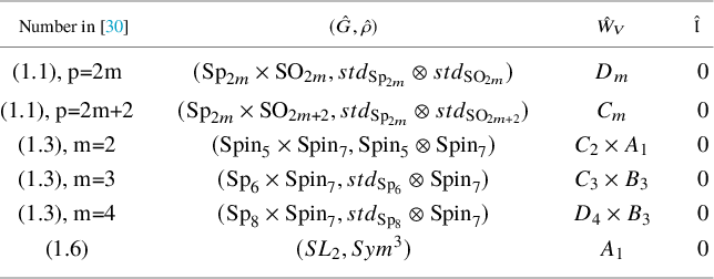
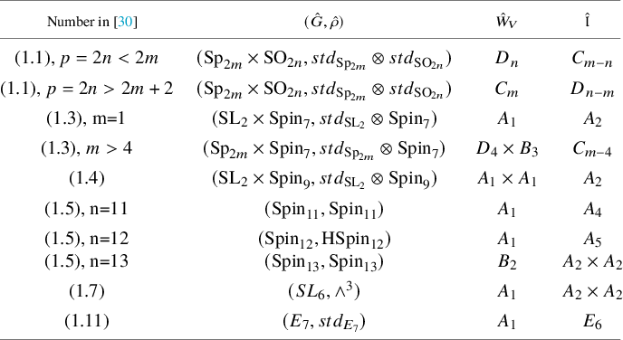
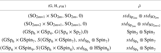


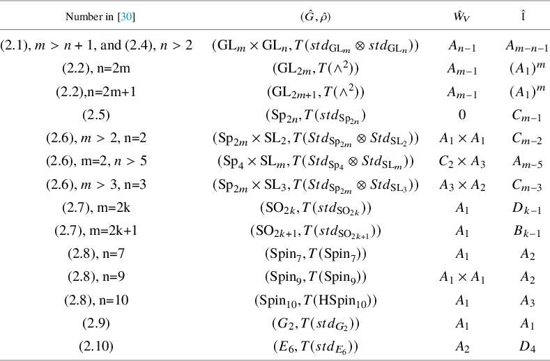


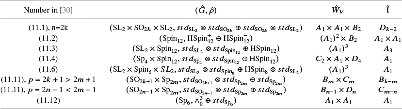


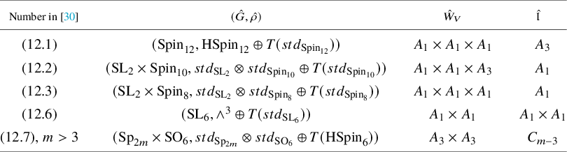

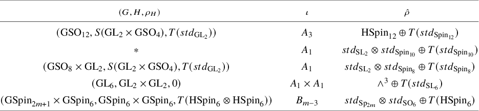


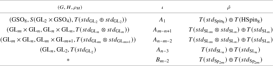

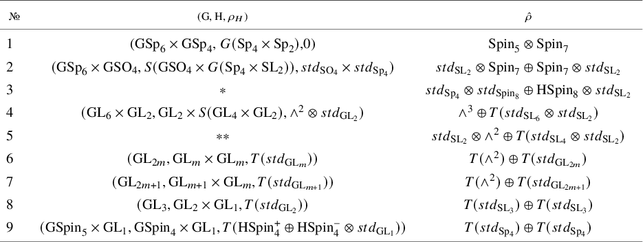
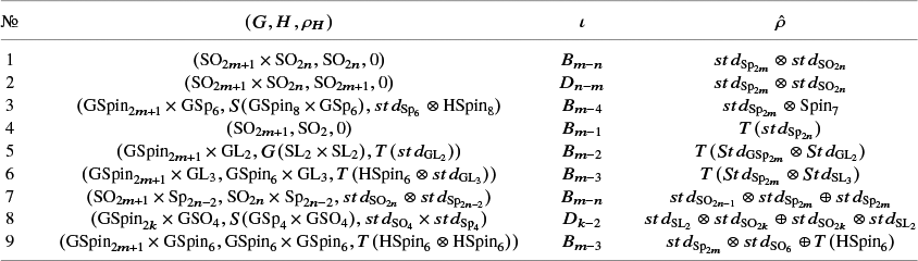
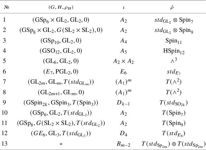
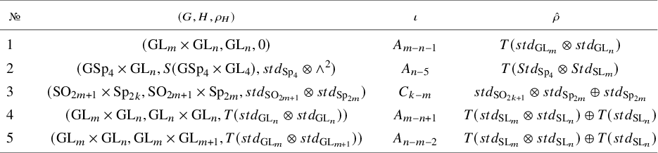
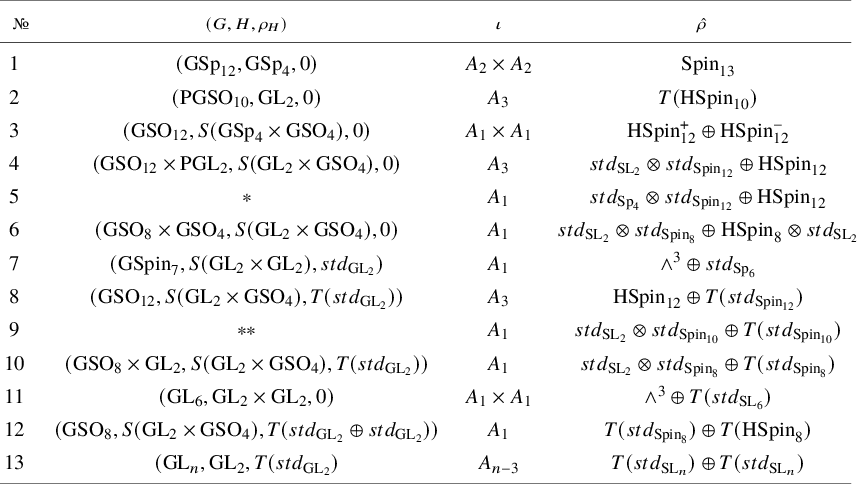


 Open access