


1. Introduction
Since Bernanke and Gürkaynak (Reference Bernanke and Gürkaynak2001) and Gollin (Reference Gollin2002) documented that the labor share of national income is uncorrelated with output per person across a large number of countries, this fact has become a standard feature of macroeconomic models, with broad implications for the shape of the production function, inequality, and cross-country comparisons.Footnote 1 What’s more, even studies seeking to understand outcomes at the sectoral level, such as which sectors are responsible for developing countries’ low productivity, generally assume that the steadiness of the national labor share carries over to sectoral labor income shares.Footnote 2 However, this aggregate steadiness might mask underlying, offsetting movements of sectoral labor shares. If such movements were systematically related to output per person, they would bias the results of studies that assume common sectoral labor shares across countries. Yet, despite their central role in economic analyses, there is a surprising lack of data on sectoral labor shares in general and whether they correlate with output per person in particular.
This paper addresses the question of whether the shares of value-added paid to labor at the sectoral level correlate with national output per person.Footnote
3
Therefore, I first create a comprehensive panel dataset of sectoral labor shares, covering several years and a wide range of development levels: The maximum value of real output per person, adjusted for purchasing power, is over 17 times larger than the minimum value (United States $\$51,119$
versus India
$\$51,119$
versus India $\$2,909$
). Then, I use panel regression techniques to analyze whether sectoral labor income shares change systematically with national output per person across and within countries and to what extent other variables, such as capital intensity and trade openness, matter for the evolution of sectoral labor shares.
$\$2,909$
). Then, I use panel regression techniques to analyze whether sectoral labor income shares change systematically with national output per person across and within countries and to what extent other variables, such as capital intensity and trade openness, matter for the evolution of sectoral labor shares.
This paper makes three main contributions. In its first contribution, it presents a novel panel dataset of sectoral labor shares that accounts for intermediate-input linkages across sectors and the labor income of the self-employed. This extends the seminal studies of cross-country national labor shares by Bernanke and Gürkaynak (Reference Bernanke and Gürkaynak2001) and Gollin (Reference Gollin2002) to a more detailed, sub-national level. Additionally, the dataset substantially increases the number of data points on sectoral labor shares by expanding the point-in-time results for the United States in 1997 by Valentinyi and Herrendorf (Reference Valentinyi and Herrendorf2008) to several countries and years. Previous studies that analyzed labor shares across countries at the sub-national level have two important limitations that this paper addresses.Footnote 4 First, the studies did not adjust for the labor income of the self-employed. Exceptions are Askenazy et al. (Reference Askenazy, Cette and Maarek2018), Decreuse and Maarek (Reference Decreuse and Maarek2017), and Bentolila and Saint-Paul (Reference Bentolila and Saint-Paul2003), which analyzed imputed labor earnings, assuming that the self-employed earn the same wages as employees. Section 3 discusses the drawbacks of this approach. This matters because Gollin (Reference Gollin2002) showed that significantly higher self-employment rates in developing countries can lead to a systematic understatement of the national labor share, potentially biasing cross-country comparisons. The second limitation is that these previous studies focused on industry-level labor shares, whereas this paper studies sectoral (or final expenditure) labor shares (e.g., the labor income share in the car manufacturing industry versus the labor income share embodied in cars). In the context of economic development, focusing on sectoral labor shares instead of industry labor shares offers at least three important advantages: first, changes in industry labor shares may reflect a relabeling of activity due to outsourcing, as opposed to shifts in economic fundamentals (e.g., van Neuss, Reference van Neuss2019). However, outsourcing does not affect sectoral labor shares because sectors incorporate intermediate-input linkages that effectively capture any outsourcing. For example, if car manufacturers shift from having in-house cleaning staff at their factories to purchasing cleaning services from an outside firm, and cleaning services have, on average, lower labor shares than car manufacturers, the data will show this as an increase in the industry labor share of car manufacturers. This problem does not plague final expenditure: holding the labor share of cleaning services fixed, it does not matter whether the cleaning services were supplied in-house or outsourced, because they are implicitly reflected (via intermediate inputs) in the final expenditure labor share of cars (Herrendorf et al., Reference Herrendorf, Rogerson and Valentinyi2013). Indeed, Berlingieri (Reference Berlingieri2014) presented evidence that outsourcing can account for a sizable share of the reallocation from the manufacturing to the services sector in the United States economy between 1947 and 2002. The second advantage of the sectoral perspective is that final expenditure categories are typically more comparable across rich and poor countries than industries: for instance, ‘spending on food’ is easier to define and compare than output in the agricultural industry. This means that data on final expenditure are readily available in cross-country studies, whereas data on industry output are not necessarily available (Herrendorf and Valentinyi, Reference Herrendorf and Valentinyi2012). The third advantage of considering labor shares in final expenditure categories is the close link to consumer preferences in demand-driven theories of structural transformation, where changes in consumer expenditure with development lead to the reallocation of resources across sectors (e.g., Kongsamut et al., Reference Kongsamut, Rebelo and Xie2001). As clarification, consider the example of a book. From an industry-output perspective, a book represents consumption of wood from forestry, processing from manufacturing, and retail services from the retail industry. In the case of final expenditure, the book represents consumption of manufactured goods. In demand-driven theories of structural transformation, consumers care about the final expenditures perspective; thus, internal consistency dictates sectoral production functions that require information on sectoral labor income shares to discipline functional forms and parameters (Herrendorf et al., Reference Herrendorf, Rogerson and Valentinyi2013).
The second contribution of this paper is to analyze the relationship between sectoral labor shares and output per person. In contrast to the standard assumption in the macroeconomic literature, I find that sectoral labor shares significantly correlate with output per person both across and within countries; the steadiness of the national labor share does not carry over to the sectoral level.Footnote 5 This finding suggests that macroeconomic studies that rely on the assumption of common sectoral labor shares across countries may yield biased results. The labor shares of the manufacturing and the services sectors evolve significantly differently with economic development compared to the labor share of the other sectors (agriculture, mining, construction, and utilities), leading to a shift in labor income between sectors as countries grow more prosperous. Additionally, while the labor share dynamics in the manufacturing sector are relatively homogeneous, the services sectoral labor shares display a significant degree of heterogeneity: Labor shares of the market services sector (e.g., communication and transport services) rise compared to non-market services (e.g., health and social services) as output per person increases. These results are informative for macroeconomic models that analyze the determinants of structural change and that examine which sectors are responsible for the low productivity in developing countries. Moreover, these findings identify sectors that, all else equal, tend to reduce inequality in society over the course of economic development: the manufacturing and market services sectors.Footnote 6 This matters because inequality can fuel social conflict, and recent research suggests it can also harm economic growth (Halter et al., Reference Halter, Oechslin and Zweimüller2014).
In the third contribution, this paper provides evidence on the channel through which development and sectoral labor shares are linked. In line with evidence on the within-country evolution of national labor shares (Karabarbounis and Neiman, Reference Karabarbounis and Neiman2014) and industry-level labor shares (Bentolila and Saint-Paul, Reference Bentolila and Saint-Paul2003), I find that the capital-to-labor ratio significantly correlates with sectoral labor shares not only within but also across countries. Intuitively, in a competitive world where sectoral production functions are not Cobb-Douglas, changes in sectoral labor shares are exclusively related to capital deepening and hence reflect changes in the relative prices of capital and labor. The link between capital deepening and sectoral labor shares is significantly more positive in the manufacturing and market services sectors than in the other sectors. These facts are consistent with the findings of Alvarez-Cuadrado et al. (Reference Alvarez-Cuadrado, Van Long and Poschke2018), who argued that multisector models should incorporate production functions with non-unitary elasticities of substitution that differ across industries. All the findings are robust to controlling for other relevant factors that the literature frequently uses to explain the movement of national labor shares, including trade openness (Elsby et al., Reference Elsby, Hobijn and Şahin2013; Harrison, Reference Harrison and Harrison2022; Jayadev, Reference Jayadev2007; Stockhammer, Reference Stockhammer2017), union density or worker-bargaining power (Askenazy et al., Reference Askenazy, Cette and Maarek2018; Fichtenbaum, Reference Fichtenbaum2011), and product market price-setting power (Blanchard and Giavazzi, Reference Blanchard and Giavazzi2003; De Loecker and Eeckhout, Reference De Loecker and Eeckhout2018; Diez et al., Reference Diez, Leigh and Tambunlertchai2018).
The finding that meaningful heterogeneity exists between market and non-market services is not new, though it has not previously been documented for labor shares. For example, Baumol et al. (Reference Baumol, Blackman and Wolff1985) found that labor productivity growth in the United States varies greatly across service-sector sub-industries. Duarte and Restuccia (Reference Duarte and Restuccia2020) emphasized the importance of accounting for heterogeneity in the services sector when analyzing sectoral productivity differences. In their study, Duarte and Restuccia (Reference Duarte and Restuccia2020) focused on intermediate input shares and relative price differences within the services sector, so they had nothing to say about non-service activities and sectoral labor shares.
Another literature to which this paper relates has shown that labor shares evolve differently within industries over time in the United States (Elsby et al., Reference Elsby, Hobijn and Şahin2013; Jones, Reference Jones2003; Young, Reference Young2010). Specifically, Elsby et al. (Reference Elsby, Hobijn and Şahin2013) found that the labor share in manufacturing industries declined substantially more than in the services industries in the United States during 1987–2011, and Young (Reference Young2010) documented the same pattern for the period 1958–1996, whereas Jones (Reference Jones2003) found the opposite during 1960–1996. Rodríguez and Jayadev (Reference Rodríguez and Jayadev2013) used United Nations National Accounts Data and found that most industry labor shares show statistically significant negative time trends. All these studies focused on within-country industry-level outcomes, so they are silent about sectoral labor shares and their evolution across countries.
Finally, two relevant papers have studied the correlation between income shares and output per person across countries in the manufacturing industry. Ortega and Rodríguez (Reference Ortega and Rodríguez2006) analyzed United Nations data on manufacturing sub-industries and found that the capital income shares in the manufacturing industry are decreasing with income across countries. Recently, Maarek and Orgiazzi (Reference Maarek and Orgiazzi2020), analyzing the same United Nations data, found a clear U-shaped pattern with development: manufacturing labor shares first decline with output per person, then rise again. An advantage of these studies is their data coverage, which includes some of the least-developed economies. I extend these studies by accounting for intermediate input linkages and labor income of the self-employed, and by documenting the evolution of other sectors, such as services, which typically account for larger shares of economic activity and employment across countries than manufacturing.
This paper is organized as follows. Section 2 outlines the methodology for mapping labor shares by industry into final expenditure using input–output tables. Section 3 describes the data sources used and discusses the different adjustments for the labor income of the self-employed. Section 4 analyzes the relationship between sectoral labor shares and output per person. Section 5 discusses to what extent capital deepening and other possible factors can account for the findings, and Section 6 concludes.
2. Method—Linking industries and sectors
In the real world and the data, industries use capital, labor, and intermediate inputs to produce both output for final expenditure and intermediate inputs for other industries. Moreover, industries may produce multiple outputs, and different industries may produce the same output. In other words, the use of intermediate inputs leads to a whole chain of intersectoral linkages that one must consider to compute the sector of final expenditure labor shares. Establishing a mapping between industries in the data and final expenditure, therefore, requires additional information about industry output and labor income as well as intersectoral linkages through intermediate inputs. Given the necessary information, one can first compute the industry labor shares and then subsequently collect all the industry labor shares that belong to a particular final expenditure sector, both directly because the industry delivers final output to that sector and indirectly through the provision of intermediate inputs to other industries whose output belongs to that particular sector. The remainder of this section describes the method in detail, closely following Valentinyi and Herrendorf (Reference Valentinyi and Herrendorf2008).
Suppose the economy consists of $I$
industries and
$I$
industries and $C$
commodities (goods and services), where industries combine intermediate inputs with capital and labor to produce output. Let
$C$
commodities (goods and services), where industries combine intermediate inputs with capital and labor to produce output. Let $\mathbf{W}$
denote the
$\mathbf{W}$
denote the $(C \times I)$
Make Matrix.Footnote
7
Rows are associated with commodities and columns with industries: element
$(C \times I)$
Make Matrix.Footnote
7
Rows are associated with commodities and columns with industries: element $(c, i)$
gives the share of one dollar of commodity
$(c, i)$
gives the share of one dollar of commodity $c$
that industry
$c$
that industry $i$
produces. The
$i$
produces. The $(C \times 1)$
commodity output vector
$(C \times 1)$
commodity output vector $\mathbf{q}$
shows for each commodity the total dollar value of the output of that commodity that is delivered to final expenditures and other industries as intermediate inputs. Let
$\mathbf{q}$
shows for each commodity the total dollar value of the output of that commodity that is delivered to final expenditures and other industries as intermediate inputs. Let $\mathbf{B}$
denote the
$\mathbf{B}$
denote the $(C \times I)$
Use Matrix. Entry
$(C \times I)$
Use Matrix. Entry $(c, i)$
shows the dollar value of commodity
$(c, i)$
shows the dollar value of commodity $c$
that industry
$c$
that industry $i$
uses as intermediate input per dollar of gross output that it produces. The
$i$
uses as intermediate input per dollar of gross output that it produces. The $(I \times 1)$
industry output vector
$(I \times 1)$
industry output vector $\mathbf{g}$
shows for each industry the total dollar value of the gross output of that industry. Finally, let the
$\mathbf{g}$
shows for each industry the total dollar value of the gross output of that industry. Finally, let the $(C \times 1)$
vector
$(C \times 1)$
vector $\mathbf{e}$
denote the vector of dollar expenditure for final uses. Entry
$\mathbf{e}$
denote the vector of dollar expenditure for final uses. Entry $c$
gives the final uses of commodity
$c$
gives the final uses of commodity $c$
.
$c$
.
The vectors and matrices are linked by accounting identities as follows:
 \begin{align} \mathbf q &=\mathbf{Bg}+\mathbf e \ , \end{align}
 \begin{align} \mathbf g &=\mathbf{W'q} \ . \end{align}
The first identity (1) states that the value of the total output of a commodity equals the value of this commodity used as an intermediate input in the production of gross output by the different industries plus the value of final expenditure on this commodity. The second identity (2) links the value of an industry’s gross output to the value of this industry’s commodity output that is used as intermediate inputs and for final uses.
Denote the $(I \times I)$
identity matrix by
$(I \times I)$
identity matrix by $\mathbf{1}$
. Combining the above identities to eliminate the vector of commodity outputs gives
$\mathbf{1}$
. Combining the above identities to eliminate the vector of commodity outputs gives
 \begin{equation} \mathbf g = \mathbf{W'(1-BW')}^{-1}\mathbf e \ , \end{equation}
whereby the $(I\times C)$
matrix
$(I\times C)$
matrix $\mathbf{W'(1-BW')}^{-1}$
is the Industry-by-Commodity Total Requirements Matrix. Rows are associated with industries and columns with commodities: entry
$\mathbf{W'(1-BW')}^{-1}$
is the Industry-by-Commodity Total Requirements Matrix. Rows are associated with industries and columns with commodities: entry $(i, c)$
shows the dollar value of industry
$(i, c)$
shows the dollar value of industry $i$
’s gross output required, directly and indirectly through intermediate input linkages, to deliver one dollar of commodity
$i$
’s gross output required, directly and indirectly through intermediate input linkages, to deliver one dollar of commodity $c$
to final uses.
$c$
to final uses.
For each commodity $c$
, denote by
$c$
, denote by $\mathbf e_c$
the
$\mathbf e_c$
the $(C\times 1)$
vector that records the final dollar expenditures on commodity
$(C\times 1)$
vector that records the final dollar expenditures on commodity $c$
, such that all other entries except
$c$
, such that all other entries except $c$
equal zero. Let
$c$
equal zero. Let $\alpha _{li}$
and
$\alpha _{li}$
and $\alpha _{vi}$
denote the labor income and value-added, respectively, generated per unit of industry
$\alpha _{vi}$
denote the labor income and value-added, respectively, generated per unit of industry $i$
’s gross output. Collect all the values in the
$i$
’s gross output. Collect all the values in the $(I\times 1)$
vectors
$(I\times 1)$
vectors $\mathbf{\alpha _l}$
and
$\mathbf{\alpha _l}$
and $\mathbf{\alpha _v}$
. With this notation, the share of value-added paid to labor embodied in commodity
$\mathbf{\alpha _v}$
. With this notation, the share of value-added paid to labor embodied in commodity $c$
is
$c$
is
 \begin{equation} \lambda _{c}=\frac {\mathbf{\alpha _l}'\mathbf{W'(1-BW')}^{-1}\mathbf e_c}{\mathbf{\alpha _v}'\mathbf{W'(1-BW')}^{-1}\mathbf e_c} \ . \end{equation}
Here, the vector $\mathbf{\alpha _l}'\mathbf{W'(1-BW')}^{-1}$
computes labor income in each commodity and the vector
$\mathbf{\alpha _l}'\mathbf{W'(1-BW')}^{-1}$
computes labor income in each commodity and the vector $\mathbf{\alpha _v}'\mathbf{W'(1-BW')}^{-1}$
computes value-added in each commodity. The expenditure vector
$\mathbf{\alpha _v}'\mathbf{W'(1-BW')}^{-1}$
computes value-added in each commodity. The expenditure vector $\mathbf e_c$
selects a particular commodity for which to compute the labor share. Note that using a
$\mathbf e_c$
selects a particular commodity for which to compute the labor share. Note that using a $(C\times 1)$
vector of ones computes a measure of the national labor share as a simple average over all final expenditure labor shares.
$(C\times 1)$
vector of ones computes a measure of the national labor share as a simple average over all final expenditure labor shares.
The described approach accounts for the relabeling of economic activities due to outsourcing at the industry level. However, using industry-level labor income shares to compute commodity labor income shares may introduce bias, since firms within an industry are likely heterogeneous in both their labor income shares and commodity mix.
The computed commodity labor income shares remain unbiased only if firms’ labor income shares are uncorrelated with their output supply patterns. To see this, consider an industry with two firms: Firm H (80% labor income share) and Firm L (20% labor income share), each contributing equally to industry output (50% average labor share). Both supply Chemicals and Textiles commodities.
Scenario 1 (Unbiased): If both firms produce 70% Textiles and 30% Chemicals, the commodity labor shares equal the industry average (50% each), correctly reflecting true values. This is because the Industry-by-Commodity Total Requirements Matrix uses average supply coefficients, which correctly reflect the composition of supply to final-use categories.
Scenario 2 (Biased): If Firm H produces 100% Textiles while Firm L produces 10% Textiles and 90% Chemicals, the true labor shares become 74.5% for Textiles and 20% for Chemicals. Using the industry average (50%) would underestimate the labor share in Textiles and overestimate that in Chemicals.
Therefore, the analysis below assumes that firms’ output supply patterns do not correlate with their labor income shares in value added. However, it is important to consider this limitation when interpreting the results.
For future reference, note that the method allows mapping labor and capital inputs from industries to commodities. Let $\tilde {h}_{i}$
and
$\tilde {h}_{i}$
and $\tilde {k}_{i}$
denote the labor and capital inputs per unit of industry
$\tilde {k}_{i}$
denote the labor and capital inputs per unit of industry $i$
’s gross output and collect all the values in the
$i$
’s gross output and collect all the values in the $(I\times 1)$
vectors
$(I\times 1)$
vectors $\mathbf{H}$
and
$\mathbf{H}$
and $\mathbf{K}$
, respectively. With this notation, the capital and labor inputs embodied in commodity
$\mathbf{K}$
, respectively. With this notation, the capital and labor inputs embodied in commodity $c$
are
$c$
are
 \begin{align} h_{c} & =\mathbf{H}'\mathbf{W'(1-BW')}^{-1}\mathbf 1_c \ , \end{align}
 \begin{align} k_{c} & =\mathbf{K}'\mathbf{W'(1-BW')}^{-1}\mathbf 1_c \ , \end{align}
whereby $\mathbf 1_c$
is a
$\mathbf 1_c$
is a $(C \times 1)$
selection vector with entry
$(C \times 1)$
selection vector with entry $c$
equal to one for commodity
$c$
equal to one for commodity $c$
and zero otherwise.
$c$
and zero otherwise.
3. Data
To assess the correlation between sectoral labor shares and output per person, I combine several sources to construct a panel dataset of such shares for a large cross-section of countries spanning the years 1995–2009.Footnote 8 This requires three datasets: first, labor income, value-added, and output at the industry level, the latter two being measured net of taxes and subsidies. These variables are available in the World Input-Output Database (WIOD), described in Timmer et al. (Reference Timmer, Dietzenbacher, Los, Stehrer and de Vries2015). This version of the WIOD adheres to the System of National Accounts (SNA) 1993. Second, data on industry-level “Net Operating Surplus and Mixed Income” from Eurostat, national statistics offices, and the OECD (see Online Appendix OA.A for details on the additional datasets). This variable is the sum of corporate-sector profits and the operating surplus of private unincorporated enterprises (OSPUE) net of depreciation. Third, I compute the Industry-by-Commodity Total Requirements Matrix from the Supply and Use Matrices in the WIOD to link industries to sectors.
3.1 Labor income
Labor income is the sum of two components: (1) the compensation of employees and (2) the labor income of the self-employed. Data on the first component is readily available in the WIOD, which uses national account statistics and labor force surveys to compute employees’ total compensation. However, as Krueger (Reference Krueger1999) emphasized, national account statistics do not account for the second component, labor income of the self-employed. Some share of the reported earnings of the self-employed should be attributed to labor income, with the remainder comprising returns on invested capital, land rents, or monopoly profits. Gollin (Reference Gollin2002) showed that the significantly higher self-employment rates in developing countries can lead to a systematic understatement of the national labor share in developing countries if the labor income of the self-employed is not properly taken into account. I consider three measures of the labor income share, each dealing with the labor income of the self-employed differently.
Payroll share. For the first measure, I consider only the labor income of employees in the corporate sector. Specifically, this payroll share measure of labor income can be written
 \begin{equation} \text{Labor share}=\frac {\text{corporate employee compensation}}{\text{value added} - \text{net taxes}} \ . \end{equation}
This measure has the advantage of being transparent and yielding unambiguous payments to labor, as advocated by Karabarbounis and Neiman (Reference Karabarbounis and Neiman2014). However, if the structure of employment changes with development, especially in the importance of self-employment as Gollin (Reference Gollin2002) documented, then the payroll share might be a poor approximation of the labor share. Studies of industry labor shares typically rely on this measure; see, for example, Azmat et al. (Reference Azmat, Manning and Van Reenen2012), Daudey and García-Peñalosa (Reference Daudey and García-Peñalosa2007), Maarek and Orgiazzi (Reference Maarek and Orgiazzi2013, Reference Maarek and Orgiazzi2020), Oishi and Paul (Reference Oishi and Paul2018), and Ortega and Rodríguez (Reference Ortega and Rodríguez2006).
Equal wages. Second, the WIOD contains information about the average working hours of employees and self-employed by industry, which I use to impute the same hourly wage for the self-employed as for corporate employees. Specifically, the equal wages labor income share is
 \begin{equation} \text{Labor share}=\frac {\text{corporate employee compensation}}{\text{employee hours worked}}\times \frac {\text{total hours worked}}{\text{value added} - \text{net taxes}} \ . \end{equation}
I perform this analysis separately for each year and industry to improve the imputation accuracy. This method is the same as that used by the United States Bureau of Labor Statistics to compute its headline measure of labor income. This equal wages measure will provide a good approximation of the labor share to the extent that the self-employed command wages essentially the same as those of employees in the corporate sector. It will be a poor approximation if there are systematic differences in earnings ability between employees and the self-employed. A version of this measure, using the ratio of the number of self-employed to employees instead of their worked hours, was analyzed by Bentolila and Saint-Paul (Reference Bentolila and Saint-Paul2003) and Gollin (Reference Gollin2002).
Imputed OSPUE. In national accounts statistics, the income of the self-employed is a part of OSPUE. As Gollin (Reference Gollin2002) argued, reallocating OSPUE between capital and labor of the self-employed may provide an improved measure of the labor share. One problem is that OSPUE is usually unavailable at the industry level; countries report only the sum of corporate-sector profits and the OSPUE net of the consumption of fixed capital (NOPS). Therefore, I follow Bernanke and Gürkaynak (Reference Bernanke and Gürkaynak2001) and construct an alternative measure of the labor share that combines information about the corporate share of the labor force from the WIOD with manually collected data on NOPS by industry. I derive imputed OSPUE for each industry by the following procedure: First, I compute total income as the sum of NOPS and corporate-employee compensation. Second, I multiply total income by the share of non-corporate employees in the labor force. Assuming that the non-corporate share of total income equals that of the non-corporate labor force, this last step yields the measure of imputed OSPUE. Finally, I split imputed OSPUE into labor and non-labor income, assuming the labor-income share in imputed OSPUE is the same as in the corporate sector. Specifically,
 \begin{align} \text{Imputed OSPUE} =& \ (\text{corporate employee compensation} + \text{NOPS}) \nonumber \\[2pt] &\times \left (1 - \frac {\text{employee hours worked}}{\text{total hours worked}}\right ) \ . \end{align}
Then,
 \begin{equation} \text{Labor share} = \frac {\text{corporate employee compensation}}{\text{value added} - \text{net taxes} - \text{imputed OSPUE}} \ . \end{equation}
The advantage of this approach is that it is transparent and straightforward, and it makes sense to assume that imputed OSPUE includes both capital and labor income. The disadvantage of this approach is that it implicitly assumes that income shares are the same for establishments that differ significantly in size and structure. To implement this approach, I collect data on NOPS from Eurostat, national statistics offices, and the OECD.Footnote 9
3.2 The roles of housing and depreciation
A large share of the real estate industry’s output is recorded as imputed rent paid by homeowners to themselves. Therefore, Rognlie (Reference Rognlie2015) argued that imputed rents from owner-occupied housing should be treated as a form of labor income akin to self-employed income: in part, they reflect labor by the homeowners themselves. The consequences of not accounting for this form of labor income can potentially be sizeable. For example, Rognlie (Reference Rognlie2015) showed that the rise in housing value added can explain a large portion of the decline in the aggregate labor share of the United States over the last few decades. A possible solution is to only analyze labor income in the corporate sector, as advocated by Karabarbounis and Neiman (Reference Karabarbounis and Neiman2014b) and Rognlie (Reference Rognlie2015). However, Gutiérrez and Piton (Reference Gutiérrez and Piton2020) showed that this will not fully resolve the measurement issues, because even in the corporate sector imputed rents can be a substantial share of value added. Instead, they propose to exclude all real estate activities from wages and value added. This method fully controls for housing, but it has the drawback of “over-controlling” by excluding residential real estate in addition to commercial real estate. None of this paper’s main results are notably affected by whether the wages and value-added of the real estate industry are included or excluded.Footnote 10
As is standard in the analysis of labor income shares (e.g., Elsby et al., Reference Elsby, Hobijn and Şahin2013; Karabarbounis and Neiman, Reference Karabarbounis and Neiman2014), this paper here is silent about what the residual, non-labor income part of value added net of taxes and subsidies consists of; some part will be capital income, while some other part may reflect super-natural profits. Additionally, depreciation accrues to neither labor nor capital but is included in value added (Bridgeman, Reference Bridgeman2018). While the share of value added paid to labor is unaffected by the split of residual value added, it is important to remember that a decrease (increase) in the labor share may not imply that capital owners are gaining (losing).
3.3 Supply and use matrices
The WIOD provides Supply and Use Matrices for each year from 1995 to 2011 for 40 countries.Footnote 11 This set of countries includes all major economies, accounting for more than 85% of the world’s GDP. A disadvantage of the WIOD is the lack of observations for the least developed countries, particularly Sub-Saharan Africa. However, the dataset is ideally suited for the analysis of sectoral labor shares for three main reasons: First, the WIOD is based on official and publicly available data from statistical offices to ensure high data quality and harmonization. Second, the dataset has been specifically designed to trace developments over time through benchmarking to time series of output, trade, and consumption from national accounts statistics. Dietzenbacher et al. (Reference Dietzenbacher, Los, Stehrer, Timmer and de Vries2013) described the construction and concepts of the WIOD in detail. Finally, the WIOD provides data on the quantities and prices of input factors by industry, including labor income and gross value added net of taxes and subsidies. These data are provided in the so-called Socio-Economic Accounts and can be combined with the Supply and Use Matrices as they follow the same industry classifications. I use the International Supply and Use Matrices to compute sectoral labor shares because these matrices allow me to distinguish between domestic and foreign buyers of goods and services, and between domestic and foreign suppliers of intermediate inputs. The matrices are in basic prices, and margin values are included in the trade and transport industries. This approach means that margins are treated as intermediate inputs, with the margin industries as the supplying industries. The International Use Matrix also contains information on final domestic expenditure by expenditure category. Finally, the Supply and Use Matrices provide harmonized information about intermediate input linkages between 35 industries and 59 final expenditure categories (Appendix Tables A1–A3 list the expenditure categories and industries).
3.4 The treatment of intangible capital
The WIOD, Release 2013, adheres to the SNA 1993. A key feature of the SNA 1993 is that spending on research and development (R&D) is not accounted for as formation of (intangible) capital. Instead, this spending represents an intermediate input in the production process, thereby reducing an industry’s value added by the same amount. By decreasing the denominator, higher R&D expenditure tends to increase the labor income share in value added, all else equal. Since R&D spending is primarily concentrated in some rich countries, this might be of first-order importance for the empirical relationship between economic development, labor income shares, and capital-labor ratios.Footnote 12
I have computed the shares of R&D investment in value added for the period 1995-2009 in NACE 2-digit industries using KLEMS data.Footnote 13 Online Appendix Tables OA.B3 and OA.B4 replicate the below main analysis, entirely excluding R&D-intensive industries from the Total Requirements Matrix and hence from the computation of sectoral labor shares and capital-labor ratios. Reassuringly, none of this paper’s main results are notably affected by whether these industries are included or excluded.
4. Empirical results
This section first examines the correlation between national labor share measures and economic development. It benchmarks the results using three different labor share measures (payroll share, equal wages, and imputed OSPUE) against those often found in the literature. Subsequently, this section presents evidence that sectoral labor income shares increase with output per person and discusses heterogeneity across sectors.
4.1 The national labor share
To assess how the different adjustment methods affect the association between the national labor share and the level of economic development, I use least squares to estimate
 \begin{equation} \log \big(\lambda ^{\text{GDP}}_{jt}\big)\ =\ \delta + \beta \: \log (\text{GDP}_{jt}) + \varepsilon _{jt} \ , \end{equation}
where $\lambda ^{\text{GDP}}_{jt}$
is the national labor share in country
$\lambda ^{\text{GDP}}_{jt}$
is the national labor share in country $j$
in year
$j$
in year $t$
, and
$t$
, and $\text{GDP}_{jt}$
denotes real output per person using prices that are constant across countries and over time, hereafter PPP, from the Penn World Table 10.01 (PWT), see Feenstra et al. (Reference Feenstra, Inklaar and Timmer2015). The parameter
$\text{GDP}_{jt}$
denotes real output per person using prices that are constant across countries and over time, hereafter PPP, from the Penn World Table 10.01 (PWT), see Feenstra et al. (Reference Feenstra, Inklaar and Timmer2015). The parameter $\beta$
is the income elasticity of the labor share, measuring the percentage change in the labor share associated with a 1% increase in output per person. Table 1 presents the regression results for each measure of labor income (Online Appendix Figures OA.C1A-C display the underlying data).Footnote
14
$\beta$
is the income elasticity of the labor share, measuring the percentage change in the labor share associated with a 1% increase in output per person. Table 1 presents the regression results for each measure of labor income (Online Appendix Figures OA.C1A-C display the underlying data).Footnote
14
Income elasticity estimates of the national labor share

Notes: Estimates of the income elasticity of the national labor share, $\hat {\beta }$
, from Regression (11). Log(GDP) is the log of real output per person, measured in PPP (2017 US
$\hat {\beta }$
, from Regression (11). Log(GDP) is the log of real output per person, measured in PPP (2017 US $\$$
). Standard errors in parentheses, allowing for clustering at the country level.
$\$$
). Standard errors in parentheses, allowing for clustering at the country level. $^{***}$ $p\lt 0.01$
,
$p\lt 0.01$
, $^{**}$ $p\lt 0.05$
,
$p\lt 0.05$
, $^{*}$ $p\lt 0.10$
.
$p\lt 0.10$
.
Column (1) shows that the average payroll share is only 49.1%, and this measure exhibits the relatively highest variation across time and countries. The income elasticity is positive and statistically significant: the payroll share increases by 0.193% when output per person increases by 1%, on average. If a country with a labor share equal to the sample average experienced output per person growth of 20%, the payroll labor share is predicted to increase from 49.1% to 51.0%. Consistent with the literature, adjusting for the labor income of the self-employed weakens the positive association between the labor share and the level of development. The income elasticity of the equal-wage labor share is only 0.116, but the average equal-wage labor share is almost nine percentage points higher than the average payroll share. The estimated income elasticity and the average value of the imputed OSPUE labor share fall between the other two measures. The finding that the national payroll share is increasing with development is consistent with previous studies (e.g., Gollin, Reference Gollin2002; Jayadev, Reference Jayadev2007). However, the estimated slope coefficients of the equal-wage and imputed-OSPUE labor shares are significantly positive, which contrasts with Bernanke and Gürkaynak (Reference Bernanke and Gürkaynak2001) and Gollin (Reference Gollin2002), who did not find a significant relationship between this labor share measure and economic development. By contrast, Izyumov and Vahaly (Reference Izyumov and Vahaly2015) also found that national labor income shares positively correlate with output per person. They updated Gollin’s results to the period 1990-2008 and included additional countries, using the same database as Gollin but instead analyzed imputed OSPUE.
To better understand why the results here differ from those of the majority of the literature, Figure 1A shows a comparison of the imputed-OSPUE labor share to the OSPUE labor share as documented in Gollin (Reference Gollin2002) (Table 2, p. 470). Because the sample period of Gollin’s data and the WIOD do not overlap - Gollin’s latest observation is from 1992, while the WIOD begins in 1995 - the horizontal axis uses a normalization; it expresses a country’s output per person in PPP relative to the United States in 1992 for Gollin’s sample and 1995 for the WIOD sample. The countries in the WIOD more than proportionally represent countries with low labor shares as compared to Gollin, and some of the relatively least-developed countries with high labor shares are absent from the WIOD (e.g., Burundi, Réunion, Ukraine, Vietnam). This selection tends to increase the correlation between labor shares and development in the WIOD data. As an additional check, Figure 1B compares the imputed-OSPUE labor share and the labor share in the PWT, both for 1995. The national labor shares generally match closely, and the relatively low labor shares among developing countries are visible in both datasets. These findings suggest that it is unlikely that systematic measurement differences between this paper and the earlier studies and benchmark data account for the positive relationship between national labor share and development. Instead, the differences seem driven by the selection of countries in the WIOD.Footnote 15
Benchmarking national labor income shares.
Notes: Panel A shows the national labor shares computed using OSPUE in Gollin (Reference Gollin2002) (Table 2, p. 470, “Adjustment 2”) and using imputed OSPUE here. The horizontal axis in Panel A shows a country’s real output per person relative to the United States in 1992 for Gollin’s data and 1995 for the WIOD data. Panel B compares the 1995 national labor shares in the PWT to those of the same countries in the WIOD.

Regression estimates of relative labor shares in the manufacturing and other goods sectors

Notes: Coefficient estimates $\hat {\beta }_j$
from Regression (12). Standard errors are in parentheses, allowing for clustering at the country level.
$\hat {\beta }_j$
from Regression (12). Standard errors are in parentheses, allowing for clustering at the country level. $^{***}$ $p\lt 0.01$
,
$p\lt 0.01$
, $^{**}$ $p\lt 0.05$
,
$p\lt 0.05$
, $^{*}$ $p\lt 0.10$
.
$p\lt 0.10$
.
Despite focusing on a selected set of countries, my analysis provides a unique view of sectoral labor shares across a large set of countries spanning various stages of development and all major economies, accounting for over 85% of world GDP. Importantly, the selection of countries should not affect results about relative sectoral labor shares - differences within countries between sectors - and within-country results over time. Accordingly, I confirm below that the findings for the income elasticity of sectoral labor shares hold when using only within-country variation for the estimation.
4.2 The sectoral labor shares
This section investigates the relationship between sectoral labor shares and development. Following Bernanke and Gürkaynak (Reference Bernanke and Gürkaynak2001), all analyses use the imputed-OSPUE labor shares. Initially, I allocate final expenditure to three sectors: manufacturing outputs, services, and other goods (agriculture, mining, utilities, and construction), see Appendix Tables A1–A2. Note that the national labor share is the weighted average of the underlying sectoral labor shares, with weights equal to the amount of final expenditure. Therefore, the national labor share may change as the expenditure vector shifts with development, even when sectoral labor shares are fixed. To prevent potential shifts in expenditure vectors from affecting results, I compute the national and sectoral labor shares in the following analyses using simple averages of all the underlying final expenditure labor shares. Using uniform weights marginally increases the correlation between the national labor share and development from 0.58 to 0.61 (Online Appendix Figures OA.C3A-B), suggesting that expenditure weights of final expenditure categories with relatively small income elasticities tend to increase with development.
Overview. I begin with some graphs indicating correlations before applying regression techniques. Figure 2 displays the national and sectoral labor shares. The labor shares of the manufacturing (Figure 2B) and services sectors (Figure 2C) increase at a similar rate with development; the correlation coefficients are 0.62 and 0.65, respectively, slightly exceeding the correlation of the national labor share with output per person. That is, the relative labor shares of manufacturing and services are higher in rich countries compared to developing countries. The labor share of the other goods sector also increases with development, but at a much lower rate than manufacturing and services (Figure 2D). As argued in the previous section, the positive correlations may be due to the selection of countries in the WIOD rather than a stylized fact that holds in a representative cross-section of countries. However, there is no reason to expect this country selection to affect the relative correlations between the national and sectoral labor shares.
National and sectoral labor shares.
Notes: National and sectoral labor shares for each year and country. Fitted values from regressing the respective labor share on real output per person (PPP) relative to the United States in 2007. Appendix Tables A1–A2 provide the allocation of final expenditure categories to sectors.

As argued earlier, substantial heterogeneity within the service sector has long been recognized in the literature; see, for example, Baumol et al. (Reference Baumol, Blackman and Wolff1985); Duarte and Restuccia (Reference Duarte and Restuccia2020); Elsby et al. (Reference Elsby, Hobijn and Şahin2013). To investigate whether differential patterns exist among labor shares within the services sector, I split services into market and non-market services. Non-market services include real estate, government and defense, health and social work, education, and sanitation services. Appendix A describes each non-market service in detail and explains that although the public sector typically carries out these services, private-sector companies also frequently provide these services. Market services include all other services, such as wholesale and retail trade, communication and transport services, financial intermediation, and research and development. Figure 3A displays the average labor shares of the market services sector, and Figure 3B of the non-market services sector. There is substantial heterogeneity in market and non-market services: Labor shares in the former increase more with development than those in non-market services; the correlation coefficients are 0.69 and 0.44, respectively.
Market and non-market services labor shares.
Notes: Sectoral labor shares for each year and country. See notes in Figure 2.

Regression estimates of relative labor shares in the services sector

Notes: Coefficient estimates $\hat {\beta }_j$
from Regression (12). Standard errors are in parentheses, allowing for clustering at the country level.
$\hat {\beta }_j$
from Regression (12). Standard errors are in parentheses, allowing for clustering at the country level. $^{***}$ $p\lt 0.01$
,
$p\lt 0.01$
, $^{**}$ $p\lt 0.05$
,
$p\lt 0.05$
, $^{*}$ $p\lt 0.10$
.
$p\lt 0.10$
.
Income elasticity of relative labor shares: Pooled estimates.
Notes: Coefficient estimates $\hat {\beta }_c$
from Regression (12). See Table 3 for underlying coefficient and standard error estimates. The horizontal axis shows the nominal expenditure share of the relevant commodity in GDP in the United States.
$\hat {\beta }_c$
from Regression (12). See Table 3 for underlying coefficient and standard error estimates. The horizontal axis shows the nominal expenditure share of the relevant commodity in GDP in the United States.

Figure 2 suggests that the variance of the aggregate labor income shares is higher in the poorest countries. The variance of labor shares in the richest 10% of observations is only 35% of the variance in the poorest 10%, and these findings hold qualitatively across various rich vs. poor categorizations. This fact was already documented by Gollin (Reference Gollin2002), who suggested that perhaps data quality may be a problem in poor countries. To examine to what extent measurement error can explain the higher labor share variance in poor countries, I investigate whether labor shares in sectors typically affected by more severe measurement issues (e.g., agriculture) exhibit a higher variance than those in sectors with presumably less severe measurement issues (e.g., manufacturing), see, e.g., Angrist et al. (Reference Angrist, Koujianou and Jolliffe2021).Footnote 16 The variance of agriculture labor shares in the richest 10% of observations is 82% of the variance in the poorest 10%. In contrast, the variance ratio between the richest and poorest 10% is around 90% in the presumably more accurately measured manufacturing sector. Therefore, even though the variance in agriculture is higher in poor countries than in rich countries, the relative variance difference of eight percentage points between more and less reliably measured sectors can only explain part of the story.
Regression analyses. To examine the relationship of the sectoral labor shares relative to the national labor share, I begin by computing the ratio of each final expenditure category labor share to the unweighted national labor share. Then, I estimate the following regression separately for each category
 \begin{equation} \log \big(\lambda _{cjt}/\lambda ^{\text{GDP}}_{jt}\big) \ = \ \delta + \beta _c \: \log (\text{GDP}_{jt}) + \varepsilon _{cjt} \ , \end{equation}
whereby $\lambda _{cjt}$
is the labor share in final expenditure category
$\lambda _{cjt}$
is the labor share in final expenditure category $c$
in country
$c$
in country $j$
in year
$j$
in year $t$
. The coefficient estimates
$t$
. The coefficient estimates $\hat {\beta }_c$
, as well as the sample average of each labor share, are displayed in Table 2 for the manufacturing and other goods sectors, and in Table 3 for the services sector.
$\hat {\beta }_c$
, as well as the sample average of each labor share, are displayed in Table 2 for the manufacturing and other goods sectors, and in Table 3 for the services sector.
Most of the manufacturing sector’s labor shares increase relative to the national labor share with economic development. By contrast, labor shares of the other goods sector exhibit a relative decline, which is strongest in the utilities categories (Electrical energy, gas, steam and hot water; Collected and purified water, distribution of water) and among agriculture, forestry, and fishing. The exception is construction work, which has a significantly positive coefficient estimate.
The estimates for the services sector lie in a wide range from –0.13 to 0.18. There are individual services for which the labor share systematically rises faster than the aggregate labor share with development, e.g., Computer and related services, Research and development, and Business services. In contrast, for non-market services, the labor shares generally decline relative to the aggregate labor share, e.g., Real estate, Education, Government, and Health and social work.
Figure 4 visualizes the relationship between estimates for the services sector and nominal expenditure shares. The non-market services categories account for the largest shares in nominal expenditure. This explains the above finding that the expenditure-weighted aggregate labor share displays a somewhat weaker correlation with development than the unweighted labor share.
The wide range of relative income elasticities in services, ranging from significantly positive to very negative, is an essential component of the heterogeneity in services highlighted in this paper. For comparison, relative labor shares in the manufacturing sector exhibit much less variation. The large majority shows a positive relationship with output per person, with a maximum estimate of 0.11, and the negative coefficient estimates do not fall below –0.05. The standard deviation of the coefficient estimates is over twice as large in the services sector as in manufacturing: 0.077 and 0.037, respectively.
To further analyze the relationship between development and sectoral labor shares, I estimate the following regression:
 \begin{align} \log (\lambda _{cjt})\ = \ &\delta + \beta \: \log (\text{GDP}_{jt}) + \sum _{s} \omega _s\: [ \log (\text{GDP}_{jt}) \times D_s ] + \sum _{s} \gamma _s\: D_s \nonumber \\ &+ \text{Category}_c + \text{Country}_j + \text{Year}_t + \varepsilon _{cjt} \ , \end{align}
Relative income elasticity of sectoral labor shares

Notes: Coefficient estimates from Regression (13). The dependent variable is the log labor share, pooled across final expenditure categories, years, and countries. Log(GDP) is the log of real output per person, measured in PPP (2017 US $\$$
). The excluded category is other goods. Appendix Tables A1–A2 list the allocation of expenditure categories to the manufacturing, services, other goods, market services, and non-market services sectors. Standard errors are in parentheses, allowing for clustering at the country level.
$\$$
). The excluded category is other goods. Appendix Tables A1–A2 list the allocation of expenditure categories to the manufacturing, services, other goods, market services, and non-market services sectors. Standard errors are in parentheses, allowing for clustering at the country level. $^{***}$ $p\lt 0.01$
,
$p\lt 0.01$
, $^{**}$ $p\lt 0.05$
,
$p\lt 0.05$
, $^{*}$ $p\lt 0.10$
.
$p\lt 0.10$
.
whereby $D_s$
is an indicator variable that equals one if the expenditure category
$D_s$
is an indicator variable that equals one if the expenditure category $c$
is associated with commodity sector
$c$
is associated with commodity sector $s$
. I include these sector-fixed effects in two ways: first, levels of
$s$
. I include these sector-fixed effects in two ways: first, levels of $D_s$
to capture potential persistent differences in sectoral labor shares (
$D_s$
to capture potential persistent differences in sectoral labor shares ( $\hat \gamma _s$
), and second, interaction terms of
$\hat \gamma _s$
), and second, interaction terms of $D_s$
and
$D_s$
and $\log (\text{GDP}_{jt})$
measure the relative income elasticity of the labor shares in sector
$\log (\text{GDP}_{jt})$
measure the relative income elasticity of the labor shares in sector $s$
compared to the omitted sector (
$s$
compared to the omitted sector ( $\hat {\omega }_s$
). Since the WIOD is a non-representative sample of countries, focusing on relative (within-country) income elasticities is necessary to obtain reliable estimates. To examine the potential heterogeneous effects of development on sectoral labor shares, I estimate Regression (13) with varying sector definitions. All regressions include year-fixed effects,
$\hat {\omega }_s$
). Since the WIOD is a non-representative sample of countries, focusing on relative (within-country) income elasticities is necessary to obtain reliable estimates. To examine the potential heterogeneous effects of development on sectoral labor shares, I estimate Regression (13) with varying sector definitions. All regressions include year-fixed effects, $\text{Year}_t$
, to capture business cycle effects. Some regressions additionally include category- and country-fixed effects,
$\text{Year}_t$
, to capture business cycle effects. Some regressions additionally include category- and country-fixed effects, $\text{Category}_c$
and
$\text{Category}_c$
and $\text{Country}_j$
, respectively. The former accounts for a small number of expenditure categories for which data are unavailable for a subset of years (mainly mining), whereas the country-fixed effects change the regression to a within-country analysis that only exploits differences over time.
$\text{Country}_j$
, respectively. The former accounts for a small number of expenditure categories for which data are unavailable for a subset of years (mainly mining), whereas the country-fixed effects change the regression to a within-country analysis that only exploits differences over time.
Table 4 displays the main results, whereby the omitted category in columns (2)–(5) is the other goods sector. Column (1) shows that, on average, labor shares increase with development: the estimated income elasticity is 0.162. This estimate is higher than the one presented in Table 1 because I include year-fixed effects and use simple averages to compute national labor shares, thereby preventing expenditure weights from affecting the results. The estimates of the interaction terms in column (2) show the manufacturing $(\hat {\omega }_{M})$
and services sector’s
$(\hat {\omega }_{M})$
and services sector’s $(\hat {\omega }_{S})$
excess income elasticities compared to the other goods sector
$(\hat {\omega }_{S})$
excess income elasticities compared to the other goods sector $(\hat {\beta })$
. Both coefficients are positive and statistically significant, whereas there is no evidence that the labor shares of the other goods sector (
$(\hat {\beta })$
. Both coefficients are positive and statistically significant, whereas there is no evidence that the labor shares of the other goods sector ( $\hat \beta$
) correlate with economic development.
$\hat \beta$
) correlate with economic development.
In column (3), I again split the services sector into market and non-market services. The results confirm the heterogeneity apparent from Figures 3 and 4. The labor shares in the market services sector rise significantly faster with economic development than in the other goods sector. The interaction term of non-market services with income per capita is not significant. Because some countries have not reported expenditures on some commodities in some years, the panel is unbalanced. If richer countries systematically stopped spending money on low-income elasticity expenditure categories, such as mining, this would bias the estimates. Column (4) shows that this is not a concern because controlling for possible changes in expenditure composition across countries does not notably change the estimates.
Finally, column (5) adds country-fixed effects, so the coefficients only measure the relative income elasticity within countries. The point estimate for the other goods sector decreases from 0.07 to –0.13, but remains not significantly different from zero. Importantly, the relative income elasticity estimates do not notably change: The labor shares of the manufacturing and market services sector have significantly higher income elasticities than those of the other goods and non-market services sector. However, even in the selected WIOD sample of countries, the labor income shares of the manufacturing and market services sectors are no longer increasing with development. At the usual confidence levels, I cannot reject the hypotheses that the sums of $(\hat {\beta } + \hat {\omega }_{M})$
and
$(\hat {\beta } + \hat {\omega }_{M})$
and $(\hat {\beta } + \hat {\omega }_{MS})$
each equal zero. This result aligns with the recent literature documenting a decline in labor shares in the United States and other countries over time.Footnote
17
The novel contribution here is to identify the other goods and non-market services sectors as the main drivers of this decline.
$(\hat {\beta } + \hat {\omega }_{MS})$
each equal zero. This result aligns with the recent literature documenting a decline in labor shares in the United States and other countries over time.Footnote
17
The novel contribution here is to identify the other goods and non-market services sectors as the main drivers of this decline.
The results are robust when using an alternative output-per-person measure and weighted least squares with expenditure weights.Footnote 18 The relative income elasticity estimates resulting from expenditure weights are only around half as large as the equally weighted elasticities computed. The interaction term between output per person and manufacturing remains significant, but the one between market services becomes insignificant. This finding suggests that commodities with relatively high elasticities receive a systematically lower share of aggregate expenditure than the other goods sector with development. Moreover, including sector-year interaction effects to purge the data of more unobserved heterogeneity does not notably affect any of the coefficient estimates.Footnote 19
The striking fact that emerges from Figures 3 and 4, and Table 4 is that many individual market services labor shares increase systematically faster with development than the labor shares in non-market services, which show a relative decline with development. These results hold across and within countries. Additionally, the recent decline of national labor shares over time appears driven mainly by the other goods and non-market services sectors, while manufacturing and market services labor shares are roughly constant within countries.
Correlation matrix and summary statistics

Notes: Output per person gives real output per person, measured in PPP (2017 US $\$$
); Capital-labor ratio gives the capital stock, adjusted for the flow of services, measured in capital PPPs (2017 US
$\$$
); Capital-labor ratio gives the capital stock, adjusted for the flow of services, measured in capital PPPs (2017 US $\$$
) per hour worked by employees and self-employed.
$\$$
) per hour worked by employees and self-employed.
5. Possible explanations for the empirical findings
What may explain the observed patterns in sectoral labor shares? One possible explanation is that countries do not operate the same sectoral technology, and these differences in production technologies somehow correlate with output per person. As Gollin (Reference Gollin2002) argued, this answer is not very appealing because why should the relationship between inputs and outputs suddenly shift at national borders? And if geography is so essential for sectoral production technologies, then how come sectoral labor shares differ more between the United States and Mexico than between the United States and Japan? Therefore, this section focuses on two other possible explanations: differences in sector-specific factor inputs, combined with production functions with a non-unitary elasticity of substitution, and differences across countries in the competitiveness of factor markets that create a gap between the wage and the marginal value product of labor.
5.1 The capital-labor ratio
In a competitive world where the production function is not Cobb-Douglas, changes in the labor share are exclusively related to capital accumulation and hence reflect changes in the competitive price of capital (e.g., Karabarbounis and Neiman, Reference Karabarbounis and Neiman2014). To examine the extent to which differences in sectoral capital accumulation matter for the relationship between income and sectoral labor shares, I add a proxy for sectoral capital accumulation to the regression model from the previous section. This proxy is the ratio of capital services to total hours worked by employees and self-employed within each sector, the capital-labor ratio.Footnote 20 I propose a method to compute this variable in four steps: First, I link data on total hours worked by employees and self-employed by industry to sectors using the Industry-by-Commodity Total Requirements Matrix, see Equation (5). Data on total hours by industry is directly available in the WIOD. Second, using the same linking process, I compute the capital stock for each sector using Equation (6). The WIOD provides data on the real fixed capital stocks at constant national prices by industry. Third, because the capital stock data are recorded in national currency units, I compute each sector’s share of the aggregate capital stock in the WIOD and use these capital input shares to allocate a country’s aggregate capital services in PPP from the PWT to commodities.
This method has the advantage of producing comparable capital input series even when relative capital prices differ across sectors. It will produce biased estimates if the relative capital prices across sectors systematically vary with income levels. I have analyzed capital PPPs at the industry level for a subsample of 20 countries for which capital PPPs are available in the Groningen Growth and Development Centre database (Inklaar and Timmer, Reference Inklaar and Timmer2009). I can reject the hypothesis at the usual confidence level that the industry capital PPPs relative to the aggregate capital PPP correlate with output per person, with absolute values of t-statistics typically less than one. This analysis suggests that disaggregated capital PPPs do not systematically vary with income levels for the subset of studied countries beyond the variation already captured by the aggregate capital PPPs.
Table 5 shows that the capital-labor ratio positively correlates with output per person and the national labor share. The sample size is around 2% smaller due to missing data on gross fixed capital or hours worked in the WIOD, mainly for the categories “metal ores” and “secondary raw materials”.
To examine whether differences in the capital-labor ratio can account for the behavior of the relative sectoral labor shares, I estimate the following regression model:
 \begin{align} \log (\lambda _{cjt})\ =& \ \delta + \beta \: \log (\text{GDP}_{jt}) + \sum _{s} \omega _s\: [\!\log (\text{GDP}_{jt}) \times D_s ] + \nonumber\\ &+ \beta ^k\: \log (k_{cjt}) + \sum _{s} \omega ^k_s\: [\!\log (k_{cjt}) \times D_s ] + \sum _{s} \gamma ^k_s\: D_s \\ \nonumber &+ \text{Category}_c + \text{Country}_j + \text{Year}_t + \varepsilon _{cjt} \ , \end{align}
whereby the new terms relative to Regression (13) is $k_{cjt}$
, the capital-labor ratio in expenditure category
$k_{cjt}$
, the capital-labor ratio in expenditure category $c$
in country
$c$
in country $j$
in year
$j$
in year $t$
. The coefficient
$t$
. The coefficient $\omega ^k_s$
gives, for sector
$\omega ^k_s$
gives, for sector $s$
, the relative elasticity of the labor shares with respect to the capital-labor ratio, hereafter capital-labor elasticity.
$s$
, the relative elasticity of the labor shares with respect to the capital-labor ratio, hereafter capital-labor elasticity.
Table 6 displays the results. For comparability, columns (1) and (3) repeat the estimates from the baseline Regression (13) using only labor share observations for which the capital-labor ratios are available, with and without country-fixed effects, respectively. Reassuringly, the previous findings continue to hold in this sample; the coefficient estimates in columns (1) and (3) are virtually unchanged compared to the results using the full sample.
Column (2) displays the effects of controlling for the log capital-labor ratios and their interactions with the sector-indicator variables. The striking result that emerges is that the relative income elasticities of the sectoral labor shares no longer differ from one another. Additionally, the estimated capital-labor elasticity in the other goods sector is significantly negative with $\hat {\beta }^k = -0.178$
. However, this may reflect sample selection bias, as the WIOD countries are not representative. The relative capital-labor elasticity of the manufacturing sectoral labor share
$\hat {\beta }^k = -0.178$
. However, this may reflect sample selection bias, as the WIOD countries are not representative. The relative capital-labor elasticity of the manufacturing sectoral labor share $(\hat \omega _M^k)$
is statistically significant and positive: a 1% increase in the capital-labor ratio is associated with a 0.134% increase in the manufacturing sectoral labor share relative to the other goods sector. A similar observation holds for the market services sector: labor shares associated with market services show significantly larger increases than other goods when the capital-labor ratio increases. Column (4) focuses on within-country variation. Controlling for the capital-labor ratio renders all relative income-elasticity estimates insignificant. In contrast, the relative capital-labor elasticity of the other goods sector is significantly negative, and those of the manufacturing and market services sectors are now significantly positive.Footnote
21
$(\hat \omega _M^k)$
is statistically significant and positive: a 1% increase in the capital-labor ratio is associated with a 0.134% increase in the manufacturing sectoral labor share relative to the other goods sector. A similar observation holds for the market services sector: labor shares associated with market services show significantly larger increases than other goods when the capital-labor ratio increases. Column (4) focuses on within-country variation. Controlling for the capital-labor ratio renders all relative income-elasticity estimates insignificant. In contrast, the relative capital-labor elasticity of the other goods sector is significantly negative, and those of the manufacturing and market services sectors are now significantly positive.Footnote
21
Finally, column (5) of Table 6 displays results when the regression controls for country-by-sector interaction effects instead of just for country fixed effects. This purges potentially unobserved, stable cross-country differences in labor income shares at the sector level, such as persistent labor market institutions or policies specific to a sector within a country (like manufacturing sectoral labor market policies in Germany versus Mexico). The coefficient estimates for the capital-labor ratio become somewhat larger in absolute magnitude, whereas the previous result—relative income elasticity estimates of the sectoral labor shares do not differ from one another once the regression controls for the capital-labor ratio—remains unchanged.
Relative income elasticity of sectoral labor shares, controlling for the sectoral capital-labor ratios

Notes: Coefficient estimates from Regression (14). The dependent variable is the log labor share, pooled across final expenditure categories, years, and countries. Log(GDP) is the log of real output per person, measured in PPP (2017 US $\$$
). Log(
$\$$
). Log( $k$
) is the log of the capital-labor ratio. The excluded category is other goods. Appendix Tables A1–A2 list the allocation of expenditure categories to the manufacturing, services, other goods, market services, and non-market services sectors. Standard errors are in parentheses, allowing for clustering at the country level.
$k$
) is the log of the capital-labor ratio. The excluded category is other goods. Appendix Tables A1–A2 list the allocation of expenditure categories to the manufacturing, services, other goods, market services, and non-market services sectors. Standard errors are in parentheses, allowing for clustering at the country level. $^{***}$ $p\lt 0.01$
,
$p\lt 0.01$
, $^{**}$ $p\lt 0.05$
,
$p\lt 0.05$
, $^{*}$ $p\lt 0.10$
.
$p\lt 0.10$
.
The results presented here provide important context for the findings in the previous section. Specifically, the excess elasticity of the manufacturing and market services sectoral labor shares is the result of two factors: first, capital-labor ratios across all sectors are increasing with economic development; and second, capital deepening has a relatively positive effect on the manufacturing and market services sectoral labor shares compared to those of the other goods sector. Taken together, these factors can account for both the within-country and cross-country estimates presented in the previous section.
5.2 Union density, markups, and trade openness
Online Appendix OA.D discusses to what extent union bargaining power, product market power, and trade openness might be able to explain the differences in the relative capital-labor and income elasticities of sectoral labor shares. While there is no conclusive evidence that union bargaining power, as proxied by union density, affects the correlation between the capital-output ratios and the sectoral labor shares, higher aggregate markups significantly decrease the relative labor shares of the other goods and the non-market services sector, but have a considerably smaller effect on the labor shares in the manufacturing and market-services sectors. That markups correlate with labor shares in the non-market services sector might seem surprising, given that they are called “non-market”. However, this sector also includes private companies that provide healthcare and education services, as well as property developers related to real estate services, which operate in market environments. Overall, the tendency for rising markups to accompany falling labor shares documented here dovetails with the findings in De Loecker and Eeckhout (Reference De Loecker and Eeckhout2018) and Diez et al. (Reference Diez, Leigh and Tambunlertchai2018), who argued that rising markups have played an essential role in the decline of labor shares around the world over the last three decades. More trade openness, measured as higher shares of exports and imports in GDP, significantly correlates with labor shares in the market services sector but does not affect the relative income elasticity or the capital-labor elasticity of sectoral labor shares. These findings offer a more nuanced understanding of the effects of trade compared to the results for national labor shares in the existing literature (Harrison, Reference Harrison and Harrison2022; Jayadev, Reference Jayadev2007; Stockhammer, Reference Stockhammer2017). Two related studies that present evidence on how trade openness affects labor shares at the industry level are Decreuse and Maarek (Reference Decreuse and Maarek2015, Reference Decreuse and Maarek2017). Decreuse and Maarek (Reference Decreuse and Maarek2015) found that openness is partly responsible for the decline in labor shares of the manufacturing industry within developing countries over time. For developed countries, Decreuse and Maarek (Reference Decreuse and Maarek2017) found that trade does not affect labor shares within industries over time but does lead to a reallocation of production factors to industries with relatively low labor shares. Both studies focus on within-country industry-level outcomes, which complement the results presented here for sectoral labor shares and their evolution across countries.
5.3 Implications for sectoral elasticities of substitution
Despite being unable to determine causality, the evidence presented in this section suggests that the capital-labor ratio plays an important role in understanding the documented relationship between relative labor shares and output per person within and across countries. This is consistent with the view that the evolution of labor shares mainly reflects changes in competitive prices due to capital accumulation (e.g., Bentolila and Saint-Paul, Reference Bentolila and Saint-Paul2003; Dao et al., Reference Dao, Das, Koczan and Lian2017; Karabarbounis and Neiman, Reference Karabarbounis and Neiman2014). Specifically, the empirical results suggest that sectors produce output according to a production function with non-unitary constant elasticity of substitution (CES), such that factor accumulation leads to changes in labor shares. See Alvarez-Cuadrado et al. (Reference Alvarez-Cuadrado, Van Long and Poschke2018) and Herrendorf et al. (Reference Herrendorf, Herrington and Valentinyi2015), who incorporated this mechanism into multi-sector growth models.
With CES production functions, capital and labor inputs can be either gross complements or gross substitutes. If the elasticity of the capital-labor ratio to the ratio of factor prices is greater than one, input factors are gross substitutes, and if it is less than one, they are gross complements. Intuitively, under gross complementarity, the share of income going to the inputs that are becoming relatively scarcer rises because these factors become increasingly important in the production process. Unfortunately, obtaining reliable estimates of the elasticity of substitution requires substantially longer time series than are available from the WIOD (e.g., Klump et al., Reference Klump, McAdam and Willman2007; León-Ledesma et al., Reference León-Ledesma, McAdam and Willman2010).
The literature has not yet reached a definitive conclusion on whether capital and labor more closely resemble gross complements or substitutes. On the one hand, Karabarbounis and Neiman (Reference Karabarbounis and Neiman2014) argued prominently that the decline in labor shares worldwide can be attributed to an increase in the capital-labor ratio combined with an elasticity of substitution above one. On the other hand, calibration exercises by Alvarez-Cuadrado et al. (Reference Alvarez-Cuadrado, Van Long and Poschke2018) and Herrendorf et al. (Reference Herrendorf, Herrington and Valentinyi2015) suggested that capital and labor are gross complements. In addition, a recent survey by Raval (Reference Raval and Raval2017) found that the large majority of estimates of the elasticity of substitution are below one, with a median of $0.54$
.
$0.54$
.
How can a CES production framework explain the finding that the labor shares of the manufacturing and market services sectors increase significantly faster with the capital-labor ratio than those of the other goods sector? As Appendix B formally shows, if capital and labor inputs are gross complements, a sufficient condition for the relative coefficient estimates would be that, for instance, capital-augmenting technological change was relatively faster in the manufacturing and market services sectors than in the other goods sector, all else equal. In this case, effective capital inputs grow relatively faster than effective labor inputs. This causes a more than proportional increase in the ratio of the marginal product of labor to the marginal product of capital. The increase leads to a rising labor share since production factors are paid their marginal products in competitive markets. Intuitively, the relative price of labor increases faster than the relative quantity of labor inputs demanded falls. Under gross substitutability, labor-augmenting technological change would need to be sufficiently faster in the manufacturing and market services sectors than in the other goods sector, for example, all else equal. Alternatively, if one were to assume that technological change at the sector level was neutral, both over time and across countries, the coefficient estimates would imply a lower elasticity of substitution in the manufacturing and market services sectors compared to the other goods sector. This aligns well with evidence on industry-level elasticity of substitution estimates from Herrendorf et al. (Reference Herrendorf, Herrington and Valentinyi2015), who found that the elasticity of substitution in the US agriculture industry is larger than one, whereas it is below one in the manufacturing and services sectors.
6. Conclusion
In this paper, I measure sectoral labor income shares for a large set of 38 countries over the period 1995-2009, taking into account intermediate input linkages and the labor income of the self-employed. I present evidence that sectoral labor shares systematically correlate with output per person and that the labor shares of the manufacturing and market services sectors increase significantly more with economic development than those of the non-market and other goods sectors. These findings hold across and within economies and are robust to the recently identified empirical challenge of accounting for imputed rents in the housing sector. My findings suggest that it may be reasonable to use models that give rise to constant factor shares in analyses focusing solely on rich countries; however, these models do not appear to be appropriate for studies involving the poorest countries. Instead, the sectoral labor share computed here can be used directly in development accounting exercises and to calibrate multisector models.
There are also cases in which assuming that labor shares are not systematically related to output per person may yield incorrect answers. For instance, when Caselli (Reference Caselli and Caselli2005) conducted a development accounting exercise using a CES production function, assuming that labor shares do not correlate with output per person, the data indicate that poor countries utilize physical capital more efficiently than rich countries. This counterintuitive result arises in his setting because a high output-capital ratio implies that capital is used efficiently, and the output-capital ratio decreases as income per person rises. In contrast, the correlation between the efficiency with which capital is utilized and income per person becomes positive when allowing for a positive correlation between labor shares and output per person. This requires that labor and capital are sufficiently strong complements in the CES production function, which seems not unreasonable based on the available evidence (Caselli, Reference Caselli and Caselli2005).
The capital-labor ratio exhibits a significant correlation with sectoral labor shares both across and within countries. Moreover, once the regression models control for the sectoral capital-labor ratios, the excess sensitivity of the manufacturing and market services sectoral labor shares with respect to output per person vanishes. This is because the link between capital deepening and sectoral labor shares is significantly more positive in the manufacturing and market services sectors than in the other sectors. By contrast, accounting for union density, product market markups, and trade openness does not notably affect the correlations between sectoral labor shares and economic development or capital-labor ratios. Taken together, these findings suggest that the capital-labor ratio is important for understanding the relationship between relative labor shares and output per person within and between countries. This is consistent with the view that the evolution of labor shares mainly reflects changes in competitive prices due to capital accumulation rather than deviations from the competitive benchmark. Several forces may be driving up aggregate savings relative to labor in more developed countries, leading to higher capital-to-labor ratios. Alternatively, Karabarbounis and Neiman (Reference Karabarbounis and Neiman2014) stressed the role of falling prices for investment goods; in their account, lower prices lead to more aggregate capital investment and, ultimately, capital deepening. However, investigating the sources of the differences in capital intensity is beyond the scope of this paper.
While the studied sample of countries covers a wide range of development levels, the analysis does not include some important regions that have typically been the focus of the development literature, such as Sub-Saharan Africa. Expanding the set of sectoral labor shares to include more countries, particularly the least-developed ones, is a promising avenue for future research.
Supplementary material
The supplementary material for this article can be found at https://doi.org/10.1017/S1365100526101011.
Competing interests
The author declares none.
Appendix A. Further details of the data
A.1 Final expenditure classification
According to the 2002 version of the statistical classification of products by activity (CPA) in the European Economic Community, the expenditure categories included in non-market services are described as:
Classification of expenditure categories - Manufacturing and Other Goods

Notes: Classification according to the 2002 version of the statistical classification of products by activity (CPA) in the European Economic Community. See: https://ec.europa.eu/eurostat/web/products-manuals-and-guidelines/-/ks-44-02-610-1f.
Classification of expenditure categories - Market and Non-Market Services

Notes: Classification according to the 2002 version of the statistical classification of products by activity (CPA) in the European Economic Community. See: https://ec.europa.eu/eurostat/web/products-manuals-and-guidelines/-/ks-44-02-610-1f.
Classification of industries

Notes: Codes follow the International Standard Industrial Classification of All Economic Activities (ISIC) Rev. 3.
CPA 70: The activities of real estate services are very diverse: real estate agents rent or sell on a commission basis; traders buy and sell property; valuers, facilities, and estate managers provide professional services; owners let property; and finally, it includes imputed rents of owner-occupied dwellings. Most of these activities relate to the secondary market, which concerns existing property. However, some, such as property developers, are active in the primary market and are more closely related to construction.
CPA 75: This section includes activities of a governmental nature, typically carried out by the public administration. This consists of the enactment and judicial interpretation of laws and their pursuant regulation, as well as the administration of programs based on them, legislative activities, taxation, national defense, public order and safety, immigration services, foreign affairs, and the administration of government programs. The legal or institutional status is not, in itself, the determining factor for an activity to belong in this section rather than the activity being of a nature specified in the previous paragraph. This means that activities classified elsewhere in NACE do not fall under this section, even if carried out by public entities. For example, administration of the school system (i.e., regulations, checks, curricula) falls under this section, but teaching itself does not (CPA 80), and a prison or military hospital is classified as health (CPA 85). Similarly, non-government units may carry out some activities described in this section.
CPA 80: This section includes education at any level or for any profession. The instructions may be oral or written and may be provided by, for example, the internet. It includes education by driving schools and the different institutions in the regular school system at different levels, as well as adult education, literacy programs, etc. Also included are military schools and academies, prison schools, etc., at their respective levels. The section includes public as well as private education.
CPA 85: This section includes the provision of health and social work activities. Activities include a wide range of activities, from health care provided by trained medical professionals in hospitals and other facilities to residential care activities that still involve a degree of health care activities to social work activities without any involvement of health care professionals. Dental and veterinary practice services are also included.
CPA 90: This section includes activities related to the management (including collection, treatment, and disposal) of various forms of waste, such as solid or non-solid industrial or household waste, as well as contaminated sites. The output of the waste or sewage treatment process can either be disposed of or become an input into other production processes. Water supply activities are also grouped in this section since they are often carried out in connection with, or by units also engaged in, sewage treatment.
Appendix B. Further details on the capital-labor ratio
To clarify how factor accumulation can account for the empirical findings, suppose that there are four sectors: manufacturing, market services, non-market services, and other goods, $s=\{M, MS, NMS, OG\}$
, respectively. Each sector produces output according to a possibly sector-specific constant-elasticity-of-substitution (CES) function:
$s=\{M, MS, NMS, OG\}$
, respectively. Each sector produces output according to a possibly sector-specific constant-elasticity-of-substitution (CES) function:
 \begin{equation} Y_s = \left [\phi _s\left (A_{s} L_s\right )^{\frac {\sigma _s-1}{\sigma _s}}+(1-\phi _s)\left (B_{s} K_s\right )^{\frac {\sigma _s-1}{\sigma _s}}\right ]^{\frac {\sigma _s}{\sigma _s-1}}, \end{equation}
whereby $L_s$
and
$L_s$
and $K_s$
are labor and capital used in sectors
$K_s$
are labor and capital used in sectors $s$
,
$s$
, $\phi _s$
governs the relative importance of the factor inputs, and
$\phi _s$
governs the relative importance of the factor inputs, and $\sigma _s\in (0,\infty )$
is the elasticity of substitution between capital and labor, defined by
$\sigma _s\in (0,\infty )$
is the elasticity of substitution between capital and labor, defined by
 \begin{equation} \sigma _s\equiv \frac {\partial k_s}{\partial \omega } \frac {\omega }{k_s}, \end{equation}
where the ratio of real wages to the rental rate of capital, $\omega$
, is the same across sectors. When
$\omega$
, is the same across sectors. When $\sigma _s\gt 1$
, the factors are gross substitutes, and when
$\sigma _s\gt 1$
, the factors are gross substitutes, and when $\sigma _s\lt 1$
, they are gross complements.
$\sigma _s\lt 1$
, they are gross complements. $A_{s}$
denotes the level of labor-augmenting technology, and
$A_{s}$
denotes the level of labor-augmenting technology, and $B_{s}$
denotes capital-augmenting technology. Therefore, the terms
$B_{s}$
denotes capital-augmenting technology. Therefore, the terms $\left (A_{s} L_s\right )$
and
$\left (A_{s} L_s\right )$
and $\left (B_{s} K_s\right )$
are the effective labor and capital inputs in sector
$\left (B_{s} K_s\right )$
are the effective labor and capital inputs in sector $s$
, respectively.
$s$
, respectively.
Under competitive markets, input factors are paid their marginal products, such that the ratio of factor shares is
 \begin{equation} \frac {\lambda _s}{\kappa _s} = \frac {\phi _s}{1-\phi _s} \left (\frac {B_{s}}{A_{s}}\right )^{\frac {1-\sigma }{\sigma _s}} \left (\frac {K_s}{L_s}\right )^{\frac {1-\sigma _s}{\sigma _s}}, \end{equation}
with $\kappa _s$
and
$\kappa _s$
and $\lambda _s$
denoting the capital and labor share in sector
$\lambda _s$
denoting the capital and labor share in sector $s$
, respectively. Under the standard assumption that
$s$
, respectively. Under the standard assumption that $\phi _s$
does not systematically vary with development, Equation (B.3) clearly predicts when sectoral labor shares will increase with the capital-labor ratio. There are two different sets of conditions, depending on whether the input factors are gross substitutes or complements. Taking logs and differentiating yields
$\phi _s$
does not systematically vary with development, Equation (B.3) clearly predicts when sectoral labor shares will increase with the capital-labor ratio. There are two different sets of conditions, depending on whether the input factors are gross substitutes or complements. Taking logs and differentiating yields
 \begin{equation} \Delta \log (\lambda _s/\kappa _s) = \frac {1-\sigma _s}{\sigma _s}\Delta \log (B_{s}/A_{s})+\frac {1-\sigma _s}{\sigma _s}\Delta \log (K_s/L_s)\ . \end{equation}
Under gross complementarity, $\sigma _s\lt 1$
, an increase in the capital-labor ratio will lead to a rising labor share as long as
$\sigma _s\lt 1$
, an increase in the capital-labor ratio will lead to a rising labor share as long as $\Delta \log (K_s/L_s)\gt -\Delta \log (B_{s}/A_{s})$
. In this case, effective capital inputs grow relatively faster than effective labor inputs, which increases effective capital per effective unit of labor. This induces a more than proportional increase in the ratio of the marginal product of labor to the marginal product of capital. Since production factors are paid their marginal products, this causes an increase in the labor share. Under gross substitutability,
$\Delta \log (K_s/L_s)\gt -\Delta \log (B_{s}/A_{s})$
. In this case, effective capital inputs grow relatively faster than effective labor inputs, which increases effective capital per effective unit of labor. This induces a more than proportional increase in the ratio of the marginal product of labor to the marginal product of capital. Since production factors are paid their marginal products, this causes an increase in the labor share. Under gross substitutability, $\sigma _s\gt 1$
, the sign of the inequality reverses.
$\sigma _s\gt 1$
, the sign of the inequality reverses.
How could the finding that the labor shares of the manufacturing and market services sectors increase at a significantly faster rate with the capital-labor ratio than those of the other goods sector be explained in this framework? Under gross complementarity, this requires
 \begin{equation} \Delta \log \left (\frac {B_{M}\: K_{M}}{A_{M}\: L_{M}}\right ) \gt \Delta \log \left (\frac {B_{OG}\: K_{OG}}{A_{OG}\: L_{OG}}\right ), \end{equation}
and
 \begin{equation} \Delta \log \left (\frac {B_{MS}\: K_{MS}}{A_{MS}\: L_{MS}}\right ) \gt \Delta \log \left (\frac {B_{OG}\: K_{OG}}{A_{OG}\: L_{OG}}\right ), \end{equation}
which say that the ratio of effective capital to effective labor must increase faster in the manufacturing and market services sectors than in the other goods sector. This would be the case, for instance, if capital-augmenting technological change was relatively slower in the other goods sector, all else equal. The case of gross substitutes reverses the sign. In this case, the ratio of effective capital to effective labor must increase more slowly in the manufacturing and market services sectors than in the other goods sector.
Alternatively, if one were to assume that the ratio $B_s/A_s$
were constant across sectors, both over time and across countries, then
$B_s/A_s$
were constant across sectors, both over time and across countries, then $\Delta \log (B_{s}/A_{s})=0$
in Equation (B.4). Consequently, the labor income share would increase with the capital-labor ratio as long as
$\Delta \log (B_{s}/A_{s})=0$
in Equation (B.4). Consequently, the labor income share would increase with the capital-labor ratio as long as $\sigma _s\lt 1$
, and the labor share would decline when
$\sigma _s\lt 1$
, and the labor share would decline when $\sigma _s\gt 1$
. In the case of a constant ratio
$\sigma _s\gt 1$
. In the case of a constant ratio $B_s/A_s$
, the finding that the labor shares of the manufacturing and market services sectors decrease at a significantly slower rate with the capital-labor ratio than those of the other goods sector could be explained by lower values of
$B_s/A_s$
, the finding that the labor shares of the manufacturing and market services sectors decrease at a significantly slower rate with the capital-labor ratio than those of the other goods sector could be explained by lower values of $\sigma$
in the manufacturing and market services sectors compared to the other goods sector.
$\sigma$
in the manufacturing and market services sectors compared to the other goods sector.
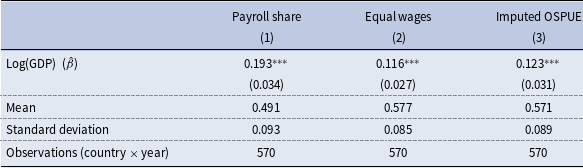

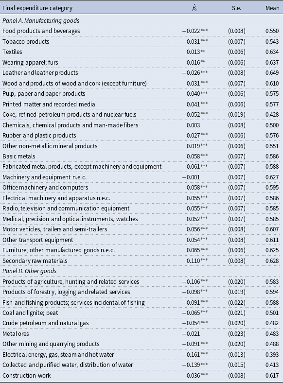


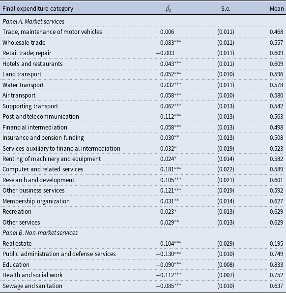


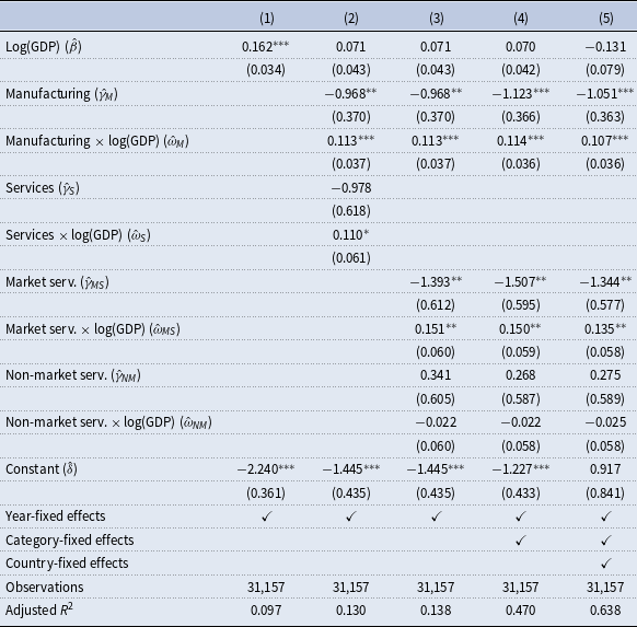
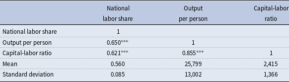
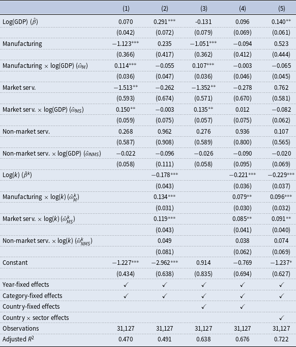
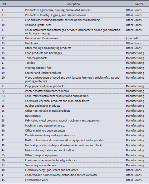
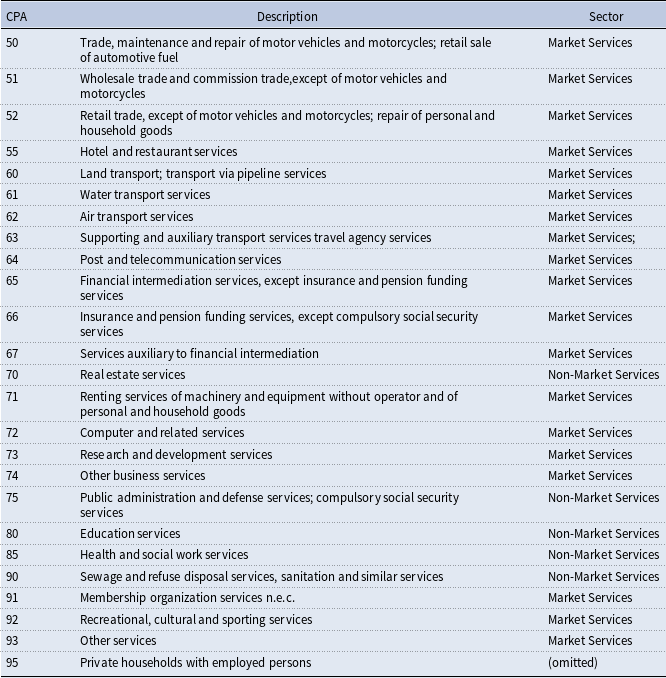
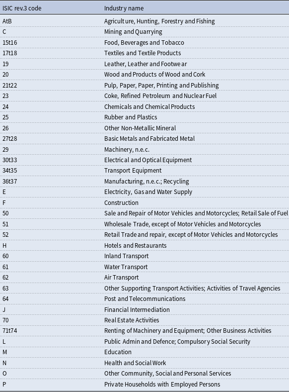


 Open access