

1. INTRODUCTION
Quaternary glaciations have left a number of geological traces on the landscape of the alps and their foreland, including glaciofluvial terraces, moraines, trimlines and scattered erratic boulders, which witness the timing and pattern of past glacier fluctuations. Such evidence has been explored and investigated for more than 200 years (Windham and Martel, Reference Windham and Martel1744; de Saussure, Reference de Saussure1779), giving birth to the theory of a single Ice Age (Perraudin, 1815, quoted in de Charpentier, Reference de Charpentier1841, p. 241; Venetz, Reference Venetz1833; Agassiz, Reference Agassiz1840; de Charpentier, Reference de Charpentier1841), followed by the identification of four glacial periods (Penck and Brückner, Reference Penck and Brückner1909), while in Switzerland at least 15 glaciations have now been identified (Schlüchter, Reference Schlüchter1988; Preusser and others, Reference Preusser, Graf, Keller, Krayss and Schlüchter2011).
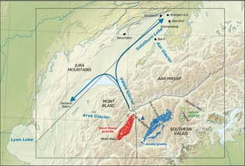
However, the more recent glaciations appear to have largely erased the older geomorphological traces, so that much of the evidence that now remains dates from the Last Glacial Maximum (LGM), which occurred ~24 000 years ago (Ivy-Ochs, Reference Ivy-Ochs2015) and is by far the best documented period throughout the glacial record. In particular, glacial evidence from this period allowed detailed maps of the LGM alpine ice cap to be drawn (e.g., Penck and Brückner, Reference Penck and Brückner1909; Jäckli, Reference Jäckli1962; Schlüchter, Reference Schlüchter2009; Ehlers and others, Reference Ehlers, Gibbard and Hughes2011), see Figure 1. In Switzerland, ice not only filled the valleys of the primary mountain range of the alps, it also covered wide parts of the foreland (Schlüchter, Reference Schlüchter2009). The upper Rhone Valley, surrounded by high mountain massifs that are still glacierized today, hosted one of the major outlets of LGM alpine ice (de Charpentier, Reference de Charpentier1841, p. 281). The Valais Glacier originated in the source area of the modern Rhone River, but it also drained the southern slope of the Bernese Alps, the northern slope of southern Valais and the eastern flank of Mont Blanc (Kelly and others, Reference Kelly, Buoncristiani and Schlüchter2004, Fig. 6). According to geomorphological reconstructions, the Valais Glacier flowed onto the foreland, where it was confined by the Jura Mountains to the north east and divided into two distributary arms (de Charpentier, Reference de Charpentier1841; Jäckli, Reference Jäckli1962; Schlüchter, Reference Schlüchter2009). One arm flowed south-westwards into the Geneva basin where it rejoined the Arve Glacier draining the western side of Mont Blanc (Coutterand, Reference Coutterand2010, Fig. 2.62; Buoncristiani and Campy, Reference Buoncristiani and Campy2011). The other distributary arm flowed to the north east and merged with the Aar Glacier to form the Solothurn lobe (Jäckli, Reference Jäckli1962; Schlüchter, Reference Schlüchter2009), see Figure 1.
Relief map of the north western alps showing the LGM extent of the alpine ice cap (blue line, after Ehlers and others, Reference Ehlers, Gibbard and Hughes2011). The arrows indicate the direction of the former ice flow from the Rhone Valley toward the Solothurn and Lyon lobes. The modelling domain (black rectangle) was divided into four precipitation zones: Mont Blanc, southern Valais, Jura Mountains and Aar Massif. Source regions of characteristic lithologies considered in this study (Mont Blanc granite, Arolla gneiss, and Allalin gabbro) are reproduced from (Swisstopo, 2005). Corresponding marker starting points used for modelling are shown by symbols ⋆, ▴ and ■. The background map consists of SRTM (Jarvis and others, Reference Jarvis, Reuter, Nelson and Guevara2008) and Natural Earth Data (Patterson and Kelso, Reference Patterson and Kelso2015).

The distribution of erratic boulders on the northern alpine foreland, in particular those on the Solothurn lobe, indicates that ice flow in the Rhone Valley during the LGM was complex (Kelly and others, Reference Kelly, Buoncristiani and Schlüchter2004). Intriguingly, many erratic boulders with lithologies characteristic of southern Valais (Arkesine, Arolla gneiss, Allalin gabbro) and Mont Blanc (Mont Blanc granites, Vallorcine conglomerate), and thus originating in tributary valleys on the left side of the Rhone Valley, were found on the LGM outline of the Solothurn lobe corresponding to the right distributary arm (Hantke, Reference Hantke1978, p. 94; Hantke, Reference Hantke1980, p. 560; Müller and others, Reference Müller, Huber, Isler and Kleboth1984, Fig. 66; Graf and others, Reference Graf2015). This indicates that boulders were transported across the centreline of the Rhone Valley. Several theories have been postulated to justify how boulders from southern Valais were diverted to the Solothurn lobe, including a strong imbalance between the contributions of the lower and upper Valais drainage basins to the glacier ice flow (Kelly and others, Reference Kelly, Buoncristiani and Schlüchter2004), or surging activities (Burkard and Spring, Reference Burkard and Spring2004).
In this paper we investigate this phenomenon (hereafter referred to as the Solothurn diversion) using an ice flow model in order to gain insight into the mechanisms governing the transport of erratic boulders. Although interpretations of the glacial record have long been restricted to qualitative analogies to modern glaciers, the recent development of scientific computing libraries (e.g., Balay and others, Reference Balay2015) and of numerical glacier models built upon them (e.g., The PISM authors, 2015) now allows for quantitative comparisons between geological reconstructions and approximated physics of glacier flow. In this study, we used the Parallel Ice Sheet Model (PISM, Bueler and Brown, Reference Bueler and Brown2009; Winkelmann and others, Reference Winkelmann2011; The PISM authors, 2015), which has been previously applied to model past glaciations on highly mountainous terrain similar to that of the alps (Golledge and others, Reference Golledge2012; Seguinot, Reference Seguinot2014; Seguinot and others, Reference Seguinot, Khroulev, Rogozhina, Stroeven and Zhang2014, Reference Seguinot, Rogozhina, Stroeven, Margold and Kleman2016; Becker and others, Reference Becker, Seguinot, Jouvet and Funk2016). In Becker and others (Reference Becker, Seguinot, Jouvet and Funk2016), the entire alpine ice cap at the LGM was modelled with PISM and constrained the precipitation pattern on the base of the geomorphological maximum ice extent. By contrast our method consists of modelling trajectories taken by boulders originating from Mont Blanc and the southern Valais in order to discover the conditions of their transport into the area formerly occupied by the Solothurn lobe.
The outline of this paper is as follows. First, the relevant information about erratic boulders of the Solothurn lobe is gathered, including their distribution, origins and dating when available. Based on this evidence, we cite several theories that have been formulated to explain the Solothurn diversion of boulders. Then we describe the ice-sheet model used, and present a range of simulations using various parametrizations of climate forcing and basal conditions. For each simulation, we compute the trajectory of erratic boulders and identify which model parametrizations are consistent with the Solothurn diversion. Finally, we assess the results against previous literature, discuss model limitations and alternative explanations.
2. SOLOTHURN DIVERSION OF ERRATIC BOULDERS
Erratic boulders deposited on the northern alpine foreland have been studied extensively since the 19th century (Agassiz, Reference Agassiz1838; de Charpentier, Reference de Charpentier1841). The granitic boulders (alpine origin) located in the Jura Mountains (predominantly limestones) played a key role in formulation of the theory of the Ice Ages (Krüger, Reference Krüger2008). It was recognized early on that the source areas of the glaciers that reached the alpine forelands can be attributed based on the lithologies of the erratics (Guyot, Reference Guyot1847; Studer, Reference Studer1832). This is possible because of the marked diversity of rocks in the alps; erratic lithologies are sometimes specific to single tributary valleys.
Crystalline rock types of the Solothurn lobe of the Valais Glacier originate from three main regions; the Mont Blanc massif, the southern valleys of the Valais and the Aar Massif, see Figure 1. Petrographic character (mineralogy and texture) generally allows distinction between the three. Mont Blanc granites are coarse-grained, equigranular to porphyritic (feldspars) and light in colour in comparison with the darker (more biotite-rich), metamorphically overprinted Aar granites and granodiorites (Spring, Reference Spring2004). In the Solothurn region Aar granites occur much less frequently than erratics of the other two types. Metamorphic rocks of the erratic population include the Arolla gneiss and the Allalin gabbro from the southern valleys of Canton Valais (Val de Bagnes, Val d'Arolla and Saastal), see Figure 1. Examples of the Allalin gabbro (outcrops in Saastal) with distinctive green pyroxenes have been reported from within the mapped extent of the LGM Valais Glacier. Clasts and boulders of Arolla gneiss of the Dent Blanche nappe (greenschist facies orthogneisses) (Mazurek, Reference Mazurek1986) are quite common. Arkesine (a local term for hornblende biotite granites and granodiorites), noted for its centimeter-long green hornblendes, is a subgroup of the Arolla gneiss.
Lithologies from the Mont Blanc region, including Mont Blanc granite and the Vallorcine conglomerate, are abundant on both sides of the Solothurn lobe (Kelly and others, Reference Kelly, Buoncristiani and Schlüchter2004; Graf and others, Reference Graf2015). Arkesine and Arolla gneiss, occur as well on both sides of the Solothurn lobe (Hantke, Reference Hantke1980; Ivy-Ochs and others, Reference Ivy-Ochs, Schäfer, Kubik, Synal and Schlüchter2004; Kelly and others, Reference Kelly, Buoncristiani and Schlüchter2004) being especially abundant on the right side at Steinhof and Steinenberg (Ivy-Ochs and others, Reference Ivy-Ochs, Schäfer, Kubik, Synal and Schlüchter2004), see Figure 1. Although sparser, Allalin gabbro erratics deposits have been found near Bern (Itten, Reference Itten1953).
It is important to confirm that the erratic boulders considered in this study were deposited during the LGM. All erratics considered here lie within the mapped and numerically dated footprint of the LGM Valais Glacier. Cosmogenic 10Be exposure dating shows that the Arolla gneiss erratics at Steinhof and Steinenberg were deposited ~24 ka (Ivy-Ochs and others, Reference Ivy-Ochs, Schäfer, Kubik, Synal and Schlüchter2004; Ivy-Ochs, Reference Ivy-Ochs2015). Along the southern slope of the Jura Mountains the Valais Glacier attained an elevation of 1100–1200 m a.s.l. near Lac Neuchâtel and descended to 600–700 m a.s.l. in the region of the terminal position near Wangen a.d. Aar (Schlüchter, Reference Schlüchter2009). During the LGM the Jura Mountains hosted an ice cap of its own. Therefore along the southern flank the two ice masses must have been in contact, see Figure 3 (right panels). Graf and others (Reference Graf2015) report LGM 10Be exposure ages for numerous erratic boulders of both Mont Blanc granite and Arolla gneiss along this line. Ages of 22–21 ka suggest that these erratics may have been deposited after the culmination of the LGM during the early stages of ice downwasting. Boulder locations mark an indistinct ice margin. Later stadial positions did not reach such a high elevation along the Jura front. Although boulders of both lithologies are also found external to the LGM left lateral position in the Jura, these must have been deposited in earlier glaciations (Graf and others, Reference Graf2015) and are not considered further here.
In our study we base lithological distribution on Mont Blanc granite, Arolla gneiss and Allalin gabbro boulders. The sheer abundance of these erratics including numerous very large ones (greater than several metres in diameter) suggests derivation from frequent rockfall onto the ice during the LGM in the accumulation areas. Based on the immense size of the boulders considered in our study and the frequency of our considered lithologies, we consider reworking of clasts from older glacial deposits unlikely.
Several theories have been formulated to explain the quasi systematic occurrence of erratic boulders from southern Valais and Mont Blanc in the Solothurn region. For instance, Kelly and others (Reference Kelly, Buoncristiani and Schlüchter2004) suggest that ice from high-elevation accumulation areas in southern Valais dominated the Valais Glacier ice flow, pushing it towards the other side of the Rhone Valley. At the Simplon Pass, striations and rat tails indicate a possible transfluence of ice from the upper Rhone Valley into the Southern Alps, which would support this hypothesis and explain the scarcity of boulders with lithologies from the upper Rhone Valley (Aar granite) on the foreland. Another explanation (Burkard and Spring, Reference Burkard and Spring2004) for the provenance of these erratic boulders involves surging activity from tributary glaciers, whose interaction with the main trunk of the Valais Glacier may have produced distorted medial moraines similar to those seen on some modern glaciers in Alaska (Meier and Post, Reference Meier and Post1969, Fig. 1) and the Karakoram (Paul, Reference Paul2015, Figs 3, 4). As the Valais Glacier fanned out onto the foreland, these distortions would have been spread out to huge proportions by the diverging flow, resulting in the highly scattered distribution of boulders observed today (Burkard and Spring, Reference Burkard and Spring2004; Coutterand, Reference Coutterand2010, p. 196–197). The goal of this paper is to assess and complete these theories by modelling the ice flow in the Rhone Valley during the LGM and analyzing the trajectories taken by erratic boulders.
3. METHODS
Our strategy consisted of running the ice flow model for different parametrizations in order to identify which parameters were compatible with a diversion of the erratic boulders from southern Valais and Mont Blanc to the Solothurn lobe. Our experiments (Exp.) tested different climate configurations (Exp. A, B, C and D in Table 1), and various parametrizations of the basal conditions (Exp. E, F, G and H). Our modelling domain consisted of a rectangle of 240 km × 190 km, which encompassed the present-day Rhone and Aar drainage basins, the Swiss Alpine foreland and the Jura Mountains (Fig. 3). In the following sections, we describe the model components used in this study, the parametrization of climate forcing, the initial conditions and the computation of boulder trajectories.
Input parameters and model results for Exp. A, B, C, D, E, G and H

Input parameters are model horizontal resolution Δx, till friction angle ϕ, basal topography, regional correction factors for precipitation (relative to present-day climate data), temperature offset ΔT and PDD factors (for snow and ice, respectively). Output data indicate the proportion of markers originating from Mont Blanc (type ⋆) and from Val de Bagnes/Arolla (type ▴) deposited in the Geneva (‘Ge’), Jura (‘Ju’) and Solothurn (‘So’) areas, as defined in Figure 3 (right panels).
3.1. Glacier model
In this study, we used the PISM (Winkelmann and others, Reference Winkelmann2011), which computes the extent and thickness of ice, its thermal and dynamic state, and the associated lithospheric response over a certain time period and for given initial basal topography and climate forcing (Fig. 2). In order to describe the dynamical motion of ice, PISM uses a linear combination of the Shallow Ice Approximation (SIA) for the vertical shear and the Shallow Shelf Approximation (SSA) for the longitudinal ice extension. In the SSA, the basal velocity and the basal shear stress are related by a pseudo-plastic power law with sliding exponent q = 0.25, threshold velocity v th = 100 m yr−1 and till cohesion c 0 = 0 Pa, see The PISM authors (2015). The yield stress is computed via a Mohr–Coulomb criterion (Cuffey and Paterson, Reference Cuffey and Paterson2010), i.e., it equals the effective pressure on the till times a till friction angle ϕ (The PISM authors, 2015). We use the values ϕ = 15°, ϕ = 30° and ϕ = 45°, which roughly correspond to the range of values measured on till (Cuffey and Paterson, Reference Cuffey and Paterson2010), see Exp. F1–F2 in Table 1. Let us note that PISM implements a polythermal version of the SIA (Bueler and Brown, Reference Bueler and Brown2009), i.e., it accounts for differences in ice softness caused by variations in temperature and water content within an ice column. These, in turn, are computed by an enthalpy formulation (Aschwanden and others, Reference Aschwanden, Bueler, Khroulev and Blatter2012), which is constrained by surface air temperature at the glacier surface and by a prescribed, constant geothermal heat flux at the glacier base of 75 mW m−2 (cf. Shapiro and Ritzwoller, Reference Shapiro and Ritzwoller2004). Finally, PISM includes a bedrock deformation model, i.e., the basal topography responds to ice load following local isostasy, elastic lithosphere flexure and viscous mantle deformation (Lingle and Clark, Reference Lingle and Clark1985; Bueler and others, Reference Bueler, Lingle and Kallen-Brown2007). The equations of momentum and energy are solved using finite differences on a regular grid, while bedrock deformation is computed by a Fourier transform. Thanks to scalable parallel solvers (Balay and others, Reference Balay2015), PISM can be run on large-scale domains with a relatively high resolution (e.g., Golledge and others, Reference Golledge2012).
Flow chart of PISM components used in this study.

The most critical component of PISM in application to our study is the surface mass-balance model, which uses climate forcing fields to provide a boundary condition to ice dynamics (Fig. 2). A positive degree-day (PDD) model (cf. Braithwaite, Reference Braithwaite1995; Hock, Reference Hock2003) computes accumulation and ablation at the surface from monthly mean surface air temperature, monthly precipitation and daily variability of surface air temperature. On the one hand, surface accumulation is equal to solid precipitation when temperature is below 0°C, and decreases to zero linearly between 0 and 2°C. On the other hand, surface ablation is computed proportionally to the number of PDD, using PDD proportionality factors f i = 8 mm °C−1 d−1 (liquid w.e.) for ice and f s = 3 mm °C−1 d−1 for snow, as in the EISMINT intercomparison experiments for Greenland (Ritz, Reference Ritz1997) in most simulations. However, since PDD factors are subject to high uncertainties, we evaluated their influence by doubling and halving their values (see Exp. E1–E2 in Table 1). The resulting ranges of f i ∈ [4, 16] and f s ∈ [1.5, 6] considered here encompass most values measured in Greenland (e.g., Braithwaite, Reference Braithwaite1995; Braithwaite and Zhang, Reference Braithwaite and Zhang2000) as well as those used by Heyman and others (Reference Heyman, Heyman, Fickert and Harbor2013) to model glacier mass balance in Central Europe during the LGM. The PDD integral (Calov and Greve, Reference Calov and Greve2005) is numerically approximated using week-long sub-intervals.
3.2. Climate forcing
During the LGM climate reconstructions indicate dry and cold conditions over Europe including mean annual temperature ~10–17°C lower than today and mean annual precipitation 60 ± 20% lower than at present (Wu and others, Reference Wu, Guiot, Brewer and Guo2007). However, the mean LGM temperatures resulting from coupled ocean-atmosphere modelling have been generally higher than those reconstructed from proxy data (Ramstein and others, Reference Ramstein2007). Strandberg and others (Reference Strandberg, Brandefelt, Kjellstrom and Smith2011) derived average LGM temperature 5–10°C cooler than present-day values in Central Europe. As a consequence, the range of uncertainties in reconstructed temperatures is still large. Yet the uncertainty in precipitation is even greater since its distribution in mountainous environments depends on orographic processes occurring on spatial scales smaller than model grids (Strandberg and others, Reference Strandberg, Brandefelt, Kjellstrom and Smith2011).
To simulate the LGM climate conditions, we used a simpler approach: we force the PDD model in PISM using corrections relative to present-day, mean monthly temperature and precipitation data bilinearly interpolated from WorldClim (Hijmans and others, Reference Hijmans, Cameron, Parra, Jones and Jarvis2005), a high-resolution global dataset built from meteorological observations and elevation data. First, we corrected the present-day distribution of mean monthly precipitation regionally to account for different precipitation patterns at the LGM. For this purpose, we divided our modelling domain into four precipitation zones: southern Valais (SV), Aar massif (AA), Mont Blanc (MB) and Jura Mountains (JU), as defined on Figure 1, and applied reduction factors c SV, c AA, c MB and c JU, respectively, between 10% and 100% in each zone, see Exp. A, B and C in Table 1. Second, we applied a single temperature offset, ΔT, which is chosen so that the maximum extent of the Solothurn lobe was modelled in the vicinity of mapped end moraines (Fig. 1). WorldClim temperatures are related to a reference present-day topography; however, we account for higher altitudes due to the build-up of ice by using an air temperature lapse rate of 6°C km−1. Spatial and seasonal temperature variability is simulated using monthly standard deviations of daily temperature computed from time series of the ERA-Interim re-analysis (Dee and others, Reference Dee2011; Seguinot, Reference Seguinot2013, Fig. 1).
3.3. Initial basal topography
In most of the simulations, initial topography was bilinearly interpolated from the present-day surface topography, including the surface of the modern glaciers and lakes, supplied as part of the WorldClim topography, which consists of a patch and aggregate of GTOPO30 (Gesch and others, Reference Gesch, Verdin and Greenlee1999) and SRTM (Jarvis and others, Reference Jarvis, Rubiano, Nelson, Farrow and Mulligan2004) data. The current glacier ice volume is negligible compared with the volume prevailing during the LGM. However, the entire Rhone Valley is presently filled with a layer of sediments up to 1 km thick, which were deposited mostly at the end of the Würm glaciation (Pfiffner and others, Reference Pfiffner1997; Hinderer, Reference Hinderer2001; Jaboyedoff and Derron, Reference Jaboyedoff and Derron2005). To account for uncertainties relating to sediment thickness in the Rhone Valley during the LGM, one of our simulations uses a reconstruction of bedrock topography from Dürst Stucki and Schlunegger (Reference Dürst Stucki and Schlunegger2013), and another uses an average of the present-day and bedrock topographies, see Exp. G1–G2 in Table 1. In fact, the bedrock topography forms a lower bound to the basal topography prevailing during the LGM, the erosion of the bedrock being negligible compared with the emptying and refilling of sediments, while the present-day surface topography forms an upper bound of the basal topography.
3.4. Computing the trajectories of boulders
In order to study the diversion of boulders to the Solothurn lobe, our strategy consisted of computing their trajectories, and analyzing the deposition zones of markers representing potential boulders travelling on the ice surface. For each characteristic lithology (Vallorcine conglomerate, Arkesine, Arolla-Gneiss and Allalin gabbro respectively), such trajectories were initialized periodically in time from each corresponding location (Mont Blanc, Val de Bagnes, Val d'Arolla and Saastal respectively), see Figure 1. We integrated forward in time the modelled surface velocity field using a fourth order Runge–Kutta method to compute the trajectory of all markers (e.g., Jouvet and Funk, Reference Jouvet and Funk2014) and identified the resulting deposition sites where each marker became immobile. Finally, the deposited markers were counted separately into three deposition zones corresponding to the Geneva basin, the Solothurn lobe and the Jura Mountains, as defined in Figure 3 (top right panel). In our analysis, we counted only boulder deposited during a period of a few millennia around the maximal state, which corresponds approximately to the total transportation times of markers (e.g., ~2.6 ka on average with ~1 ka standard deviation in Experiment B3). More precisely, this time period is defined so that the total volume of ice remained between 90% and 100% of the maximal volume. Let us note that a sufficiently large number of initial markers was chosen so that at least 200 markers from each source region were deposited during this period. Analyzing a large set of markers instead of individual ones ensured that our results were not dependent on small changes in the precise location of the source region (cf. Jouvet and Funk, Reference Jouvet and Funk2014, Fig. 5).
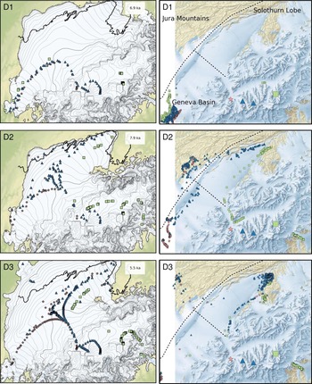
Left: Snapshots of the modelled ice extent, and markers for ‘today's precipitation pattern’ Experiment D1 (top), ‘corrected precipitation pattern’ Experiment D2 (middle) and ‘colder Jura’ Experiment D3 (bottom) at the time when the volume of ice was maximum. Symbols ⋆, ▴ and ■ represent markers initialized at Mont Blanc, Val de Bagnes/Arolla and Saastal areas. For convenience, the LGM outlines of reference Figure 1 are drawn. Right: Final deposition site of markers after being transported by the modelled ice flow for Exp. D1 (top), D2 (middle) and D3 (bottom). Large and small symbols ⋆, ▴ and ■ represent upstream initialisation and downstream deposition sites, respectively. The dashed lines indicate the separation between Geneva, Jura and Solothurn areas defined for computing the proportion of markers in Table 1 © 2016 swisstopo (JD100042).

4. RESULTS
Using various parameters for climate forcing, basal conditions and model resolution, we ran 36 simulations of glacial evolution in order to identify which parameters were compatible with a diversion of erratic boulders from the Mont Blanc and southern Valais to the Solothurn lobe during the LGM, see Table 1 and Figure 4. All simulations were initialized under ice-free conditions, and ran with given unvarying climatic conditions over a time period sufficiently long to allow the modelled ice sheet to reach its maximum extent. In the following subsections, we detail each experiment we have achieved.
Proportion of markers (in %) deposited in the Solothurn lobe (counting neither the ones that come from Saastal nor those deposited over the Jura Mountains) with respect to precipitation correction ratios c AA/c SV and c AA+/c MB, which control the rebalancing of precipitation between the Aar Basin (AA) and the southern Valais (SV), and between the latter two (c AA+ : = (c AA + c SV)/2) and Mont Blanc (MB), respectively. The contours rely on 5 × 4 grid points corresponding to 20 different simulations including Exp. A2, B1, B2 and B3, which are marked by black dots on the graphs. All model parameters (except ΔT, c SV, c AA, c MB and c JU) are analogous to those of Exp. A1–A4 and B1–B3.

4.1. Experiment A: homogeneous precipitation change
First, we considered a uniform scaling of precipitation, i.e., no change in its spatial pattern (c SV = c AA = c MB = c JU), see Table 1 (Exp. A1–A4). Although a wide range of climate configurations (ΔT ∈ [−9.4, −15.6]°C and  $c_{{\rm prec}} \in [10,100]\% $) shows similar maximum ice extents, none of the configurations allow the markers to be transported from southern Valais to the Solothurn lobe, see Table 1 (Exp. A1–A4). Instead, most of the markers were transported along a flowline following the left bank of the Rhone Valley and deposited in the Geneva basin after the modelled Valais Glacier fanned out on the flatland. This behaviour of marker trajectories is illustrated in Figure 3 (top-left panel), which displays the results of a comparable experiment.
4.2. Experiment B: local precipitation change
By contrast with previous experiments, the application of different precipitation correction factors c SV, c AA, c MB, c JU for different areas impacted the directions taken by the ice flow and, in turn, the marker trajectories, see Table 1 (Exp. B1–B3). For instance, applying twice as much precipitation over the Mont Blanc area as over the Aar Massif and the southern Valais caused the ice flowing out of the Mont Blanc massif to create an ice jam in the Geneva basin. In this situation, the modelled ice flow of Valais Glacier was partially diverted towards the Solothurn lobe so that some of the markers from Val de Bagnes and Val d'Arolla were deposited along the southern edge of the Jura Mountains, while most of the markers originating from Mont Blanc were again deposited in the Geneva basin, see Experiment B2 in Table 1. However, applying an additional reduction of precipitation over the Aar Massif relative to southern Valais prevented the Aar Glacier from obstructing the right arm of the Valais Glacier, so that markers from both Mont Blanc and southern Valais were deposited in the Solothurn lobe, see Experiment B3 in Table 1. More generally, Figure 4 shows the proportion of markers deposited in the Solothurn lobe for 20 different simulation runs, which explore different combinations of precipitation corrections. As a result, the enhancement of precipitation over Mont Blanc appears more critical to the diversion of the markers to the Solothurn lobe than the dampening of precipitation over the Aar Massif relative to southern Valais, which alone had no effect (Experiment B1 in Table 1).
4.3. Experiment C: global and local precipitation change
In the next experiment, we applied a global increase or decrease of precipitation relative to the precipitation pattern favourable to the diversion of markers used in Experiment B3 and temperature adjusted accordingly. As a matter of fact, the total input precipitation affected the marker trajectories. Indeed, increased total precipitation and temperature caused fewer, while decreases caused more, markers to be diverted to the Jura Mountains and to the Solothurn lobe (Table 1, Exp. C1–C3).
4.4. Experiment D: spatial model resolution
The spatial model resolution is a critical model parameter, which controls how well the complex topography of the alps is captured. While Exp. A–C used a 2 km horizontal resolution, Exp. D1 and D2 used a finer horizontal resolution of 1 km, and other parameters similar to Exp. A2 and B3. Using the present-day precipitation pattern, the lack of markers deposited in the Solothurn lobe could not be recovered by the increased horizontal resolution (Table 1, Exp. A2 and D1 ; Fig. 3 top panels). By contrast, using the precipitation pattern favourable to the diversion, refining the resolution from 2 to 1 km revealed a reduction in the proportion of markers from Mont Blanc and a more scattered distribution of markers from Val de Bagnes and Val d'Arolla deposited on the Jura Mountains and in the Solothurn lobe (Table 1, Exp. B3 and D2 ; Fig. 3, middle panels). Finally, Experiment D3 used a similar setup as Experiment D2, but included an additional cooling of 2°C on the Jura Mountains in order to generate an independent ice cap there. As a result, a small self-sustained ice cap appears on the Jura Mountains in the early stages of the simulation before merging with the Valais Glacier. This initial thickness of ice on Jura Mountains increased substantially the number of markers diverted to the Solothurn lobe, see Table 1 (Experiment D3) and Figure 3 (bottom panels).
By contrast with markers from Mont Blanc, Val de Bagnes and Val d'Arolla, the ones originating from the eastern-most location, Saastal, were considered only in the 1 km-resolution experiments (Experiment D). Indeed, an ice divide appears at the intersection between the Saastal and the Rhone Valleys (Fig. 1) in the 2 km-resolution experiments so that all markers from Saastal are carried south-eastwards to Italy instead of westwards down the Rhone Valley. As a matter of fact, the 1 km-resolution experiment resolves the basal topography better so that the modelled ice divide is shifted eastwards, allowing part (but not all) of the markers to be transported westwards. The latter are transported along the right valley side, and are deposited along the right side of the Solothurn lobe (see Fig. 3).
4.5. Experiment E: PDD factors
The choice of PDD factors strongly impacts the computation of surface mass balance and the resulting modelled extent. However, doubling or halving the PDD factors, and accordingly adjusting the temperature offset ΔT to match the mapped LGM ice extent, did not impact the final distribution of markers when using today's precipitation pattern, see Exp. E1–E2 in Table 1.
4.6. Experiment F: basal motion
Other parameter choices unrelated to climate might have consequence for the final distribution of markers. For instance, the basal friction angle, ϕ, which controls the modelled sliding velocity, was difficult to constrain since the magnitude of the LGM alpine ice flow cannot be directly measured. However, using the present-day precipitation pattern, increasing or decreasing the basal friction angle within the range of values measured on glacial sediments had no consequence on the final distribution of markers (Table 1, Exp. F1–F2).
4.7. Experiment G: basal topography
To account for partial removal of glacio-fluvial sediment from the overdeepened valleys, we ran PISM not only using the present-day topography (Table 1, Experiment A2), but also using the bedrock (Table 1, Experiment G1) and the average of both (Table 1, Experiment G2). However, changing the basal topography alone could not cause any diversion of the markers (Table 1 Exp. G1–G2) when using today's precipitation pattern.
5. DISCUSSION
We have considered two kinds of geological information in order to constrain the climate conditions prevailing during the LGM. First, we used the reconstructed glacial extent based on moraines to corroborate a set of global precipitation corrections and corresponding temperature offsets. Second, we refined our results, especially the spatial distribution of precipitation, by exploiting the source regions and deposition zones of glacial erratic boulders.
5.1. Global insights about the LGM climate
The input climates compatible with the geomorphologically reconstructed LGM extent and the diversion of boulders to the Solothurn lobe include a spatially-average cooling of 9.4–13.2°C and a reduction of precipitation of 0–75% with respect to the present-day climate (Exp. B3, C1, C2, D1, D2 and D3). These temperatures are consistent with previous reconstructions based on proxy data, however the range for precipitation reductions is too large to allow any direct comparison. For instance, pollen-based reconstructions (Wu and others, Reference Wu, Guiot, Brewer and Guo2007) indicate mean annual LGM temperatures ~10–17°C lower than today and mean annual LGM precipitation rates 60 ± 20% lower than at present over Europe. In addition, our results are comparable with the LGM climate reconstructions of Heyman and others (Reference Heyman, Heyman, Fickert and Harbor2013) and Allen and others (Reference Allen, Siegert and Payne2008) from the Black Forest, Vosges and Jura Mountains, which are located <200 km away from the Solothurn lobe, see Table 2. These reconstructions were obtained using a PDD model approach similar to ours (with comparable PDD factors, see Table 2), however, without accounting for ice flow dynamics, this assumption is being valid for small glaciers only. While our temperature offsets agree well with those of the Black Forest for present-day precipitation scaled by 25 and 50%, the climate reconstructed by Heyman and others (Reference Heyman, Heyman, Fickert and Harbor2013) and Allen and others (Reference Allen, Siegert and Payne2008) in the Vosges and the Jura Mountains are notably cooler (up to 3°C) than our reconstructions, see Table 2.
LGM climate reconstructions in terms of temperature offsets (ΔT in °C) and precipitation scaling (c prec in %) in relation to present-day climate data

These reconstructions were obtained using a model-based approach over the Vosges and the Black Forest in Heyman and others (Reference Heyman, Heyman, Fickert and Harbor2013) and the Jura Mountains in Allen and others (Reference Allen, Siegert and Payne2008). For the sake of comparison, our results (from Table 1, Experiment B3) are reported (in bold) and the PDD parameters (f i, f s in °C−1 d−1) used for each study are stated.
5.2. Enhanced precipitation in the south west
Using the present-day precipitation pattern, the model could not produce an ice flow field diverting the trajectory of boulders originating in Mont Blanc and southern Valais to the Solothurn lobe. In fact, only a strong local increase of precipitation over Mont Blanc and southern Valais relative to the Aar Massif led to a diversion of erratic boulders to their observed deposition zone, see Figure 3. As a consequence, our results first support the theory that there were higher precipitation rates in the south than in the north of the alps at the LGM compared with today. By contrast, most of today's precipitation in the alps is associated with low-pressure systems originating in the north Atlantic, which predominantly supply the Northern Alps with moist air masses. Several studies have already shown evidence for enhanced precipitation in the Southern Alps at the LGM. For instance, Florineth and Schlüchter (Reference Florineth and Schlüchter2000) argued that the reconstruction of ice domes south of the present weather divide necessarily implies a southward-dominated precipitation regime. Recently, Becker and others (Reference Becker, Seguinot, Jouvet and Funk2016) drew similar conclusions by constraining the precipitation pattern in PISM from the geomorphological maximum ice extent, however, at the scale of the entire alps. Lastly, in Luetscher and others (Reference Luetscher2015), records of meteoric precipitation obtained from speleothems grown during the LGM support a southward shift of the north Atlantic storm track resulting in preferential advection of moisture from the south. In fact, Figure 4 indicates that the diversion was primarily controlled by an enhancement of precipitation over Mont Blanc, which caused the ice flowing out of the Mont Blanc Massif to partially hold back the Valais Glacier in the Geneva basin. This pattern is surprising since the Mont Blanc massif is located north of the alpine weather divide, but can be interpreted as being in an intermediary state between northerly- and southerly-dominant moisture advection regimes.
5.3. Enhanced cooling over the Jura Mountains
Model results obtained with 1 km horizontal resolution (Exp. D2 and D3) are most suited to analyze in detail the boulder trajectories in the configurations favourable to their diversion to the Solothurn lobe. Table 1 (Experiment D2) and Figure 3 (middle panels) show that the boulders with the eastern-most origins tend to be in larger proportion diverted to the Solothurn lobe than boulders from Mont Blanc. Indeed, the latter move along flowlines following the left valley side, which are by nature more favourably positioned to end up in the Geneva Basin than more centrally located flowlines. As a matter of fact, the deposition of metamorphic boulders (Arkesine and Arolla-Gneiss) originating in Val de Bagnes and Val d'Arolla on the left side of the Solothurn lobe (see Fig. 3) shown by the model (Experiment D2) matches well with the observations (Hantke, Reference Hantke1980; Ivy-Ochs and others, Reference Ivy-Ochs, Schäfer, Kubik, Synal and Schlüchter2004; Kelly and others, Reference Kelly, Buoncristiani and Schlüchter2004). The same conclusions are drawn for the boulders from Saastal (Allalin gabbro). The latter are deposited along the right side of the Solothurn lobe (see Fig. 3, middle panels), as shown by the finding of Allalin gabbro erratics in LGM deposits near Bern (Itten, Reference Itten1953) along the right-hand side outermost LGM ice margin. By contrast, the distribution of granitic boulders originating at Mont Blanc is more complex to analyze. In fact, none of them even reach Neuchâtel (Fig. 1) where boulders dated from LGM and originating at Mont Blanc (like the ‘Pierre-à-Bot’) were found, see Figure 3 (middle panels). By contrast, ~20% of them are modelled to be deposited west of the Jura Mountains, see Table 1 (Experiment D2). These unexpected positions (beyond the reconstructed outlines) are attributed to the absence of an independent ice cap on the Jura Mountains in our simulations (except for the coldest configuration), whereas evidence for such an ice cap does exist (Coutterand, Reference Coutterand2010). In the absence of ice, the Jura Mountains is too weak of an obstacle and cannot effectively hold back the Valais ice flow and therefore gets covered beyond the reconstructed outlines. As a result, many boulders are transported across the Jura Mountains instead of being diverted to the Solothurn lobe and deposited on the southern slope of the Jura Mountains. We conclude that the cooling must have been underestimated on the Jura Mountains, as already suggested by Table 2. This analysis is supported by Experiment D3, which includes a 2°C supplementary cooling on the Jura Mountains (Fig. 1) to the set-up of Experiment D2 so that an ice cap up to 500 m thick appears there, see Figure 3 (bottom panels). This automatically implies a more efficient diversion of boulders to the east, as indicated in Table 1 (Experiment D3) and Figure 3 (bottom panels). The presence of an ice cap over the Jura Mountains prevents boulders from being deposited along the ridge on the left side of the Solothurn Lobe where the two ice masses are in contact. Further downstream, where the two are separate, boulders can be deposited, for example at the ‘Pierre-à-Bot’ location near Neuchâtel (Graf and others, Reference Graf2015). This also suggests that the boulders along the southern slope of the Jura were deposited during the downwasting phase of the LGM when the Valais Glacier and Jura ice were no longer in contact, so after 24 000 years ago (Graf and others, Reference Graf2015).
5.4. Sensitivity to non-climatic inputs
We find the PDD factors, the basal motion parameters and the basal topography to be among the most uncertain non-climatic model inputs. However, Exp. E, F and G show that varying these inputs within a realistic range while maintaining today's precipitation pattern do not explain the diversion of the boulders to the Solothurn lobe. In particular, the use of lower basal topographies in the valleys (the bedrock or its average with the present-day surface) yield a less pronounced diversion. Indeed, removing layers of sediments from the basal topography lowers the surface along the Rhone River (which passes by Geneva) and favours boulder transport to the south. In conclusion, the Solothurn diversion of boulders cannot be explained by non-climatic factors without considering a strongly different precipitation pattern than today.
A theory involving surging activities in the southern transversal valleys of the main trunk was formulated to explain the diversion of boulders to the Solothurn lobe during the LGM. Despite some modelling attempts (results not shown) to simulate ice surges by favouring basal motion locally in the transversal valleys of the Valais Glacier, it was not possible to sustain fast ice flow while the Valais Glacier reaches its maximal extension since the trunk of the Valais Glacier obstructs the path of tributary glaciers. As a result the ice flow remains unchanged in this configuration and boulders from the Mont Blanc and southern Valais were not diverted to the Solothurn lobe. Although it is not excluded that a higher resolution model with periodical basal sliding conditions can better reproduce sustainable surging activity, it sounds unlikely that this would have caused a number of erratic boulders to be diverted to the Solothurn lobe.
5.5. Model limitations
Our result must be interpreted with care since our parametrization of the LGM climate is fairly simple. In particular, we applied a constant-in-time cooling under ice-free conditions to obtain a maximal ice coverage within a short period of time, while the build-up of the Valais Glacier resulted from a slow and irregular cooling over an entire glacial cycle (Preusser and others, Reference Preusser, Graf, Keller, Krayss and Schlüchter2011). By doing so, the modelled glacier was nearly in a steady state at the LGM, so that it was little influenced by uncertain initial conditions, and the ice flow directly reflects the climate forcing. As a consequence, this approach is suitable for evaluating the impact of relative changes in climate conditions on the trajectories of boulders; however, our estimate of absolute LGM temperatures and precipitation amounts are more uncertain since the period prior to the LGM was not modelled. Since our climate forcing was not transient but stationary, our model cannot reproduce a remobilization of boulders as for instance those re-worked by the Jurassian ice flow after being deposited by the Rhone ice flow (Graf and others, Reference Graf2015). However, reworking would have probably caused boulders to crush, and we can reasonably assume that the large-size boulders considered here were transported in a single glacier advance.
We also assumed that the LGM temperature seasonality was similar to that of the present day. As a result, increased snowfall associated with more severe winter cooling relative to the annual mean (Strandberg and others, Reference Strandberg, Brandefelt, Kjellstrom and Smith2011) might not have been captured in the model. Another limitation of our approach is that we have not considered any spatial corrections of the temperature (except in Experiment D3) as we did for precipitation. Consequently, it is possible that the strong local corrections in precipitation required to simulate boulder transport to the Solothurn lobe could be replaced by more reasonable corrections of both precipitation and temperature.
Lastly, uncertainties in the modern climate dataset WorldClim can be a limiting factor, especially in mountainous environment. For this reason, it is crucial to verify that WorldClim represents the present-day distribution of precipitation well enough, i.e. without major imbalance between the regions of the alps considered in this study. Direct comparisons with observations (see Appendix) did not reveal any strong discrepancy nor spatial imbalance between WorldClim and observed precipitation.
6. CONCLUSIONS AND PERSPECTIVES
Using the PISM (Winkelmann and others, Reference Winkelmann2011), we simulated the transport of erratic boulders by the Valais Glacier during the LGM. In order to mimic LGM climate conditions, we applied a constant offset of temperature and regionally variable precipitation correction factors to present-day climate data. Based on this set-up, we ran a set of simulations using various climate configurations, and analyzed for each of them the path followed by boulders originating from the Mont Blanc and southern Valais regions. In most simulations, all boulders were carried to the Geneva basin, and none to the Solothurn lobe. This result is inconsistent with the observation of abundant erratic boulders from Mont Blanc and southern Valais deposited by the Solothurn lobe (Graf and others, Reference Graf2015). However, applying a strong local increase of precipitation over Mont Blanc and southern Valais relative to the Aar Massif as input to the model resulted in a diversion of boulder trajectories to the Solothurn lobe during the LGM consistent with these observations. This result corroborates previous studies by Florineth and Schlüchter (Reference Florineth and Schlüchter2000), Becker and others (Reference Becker, Seguinot, Jouvet and Funk2016) and Luetscher and others (Reference Luetscher2015), which support a precipitation regime dominated by southerly moisture advection at the LGM. However, the enhancement of precipitation over the Mont Blanc Massif also indicates that a westerly preferential moisture advection also prevailed around the LGM. Indeed, it was also essential that the Mont Blanc Massif received enough precipitation so that ice flow from Mont Blanc obstructed the left arm of the Valais Glacier, and boulders from Mont Blanc and southern Valais were diverted to the Solothurn lobe. We conclude that the relative difference between precipitation rates over the Mont Blanc area and the southern Valais was higher during the LGM than it is today. In addition, our results show that for some time around the LGM the Jura Mountains must have been a few degrees colder than the rest of the study area in order to sustain an independent ice cap sufficiently thick to block the flow of the Valais Glacier across the Jura and to divert boulders originating from Mont Blanc to the east to the Solothurn lobe. Regional circulation modelling of climatic conditions prevailing over the alps during the LGM indeed results in a strongly enhanced winter precipitation gradient over the mountain range as compared with today (Strandberg and others, Reference Strandberg, Brandefelt, Kjellstrom and Smith2011, Fig. 6). However, such regional effects as implied by our study will need to be validated against circulation model results even more highly resolved than those currently available in order to elucidate their possible causes. Other model configurations have been tested to evaluate potential non-climatic triggers (basal motion or topography) of the Solothurn diversion; however, none of them were found able to model the diversion.
This study, which combines geomorphological observations and numerical modelling, is the first to our knowledge that uses erratic boulders of known origin to constrain modelled flow patterns. Our simulations show that, besides the reconstructions of maximum extent from moraines commonly used to constrain numerical models, erratic boulders of known origin provide extremely valuable and reliable information about ice flow fields that can be used to infer paleo-climatic conditions responsible for their transport routes.
ACKNOWLEDGEMENTS
We thank C. Schlüchter, an anonymous referee, D. Rippin and G. Cogley for their constructive comments, which contributed to improve the manuscript.
APPENDIX: ASSESSMENT OF WORLDCLIM DATA
WorldClim is a 1 km resolution dataset built from meteorological observations, providing monthly average mean temperature and precipitation relative to the period 1960–90 (Hijmans and others, Reference Hijmans, Cameron, Parra, Jones and Jarvis2005). Here we assess modelled snow accumulation computed from WorldClim data (i.e. solid precipitation when temperature is below 0°C, and decreases to zero linearly between 0°C and 2°C) against measurements of snow accumulation over 17 different sites (World Glacier Monitoring Service, 2012; Huss and others, Reference Huss, Dhulst and Bauder2015). These sites are located on nine glaciers of the Alps and represent four distinct regions (South-West, North Valais, South Valais and East). Table 3 displays the modelled snow accumulation rates  $\bar A_{{\rm WC}} $ computed from WorldClim data, the normalized deviation between $\bar A_{{\rm WC}} $ and the measured snow accumulation rates $\bar A_{{\rm meas}} $, and the standard deviation (STD) between the two series. For simplicity, the averaged snow accumulation values $\bar A_{{\rm WC}} $ and $\bar A_{{\rm meas}} $ over all measurement points of the same region. As a result, the WorldClim precipitation data match the measurements relatively well since the highest discrepancy is 23%. More importantly, no strong imbalance can be noticed between the different regions.
Modelled snow accumulation rates  $\bar A_{{\rm WC}} $ (in m a−1) computed from WorldClim data, normalized deviation between $\bar A_{{\rm WC}} $ and measured snow accumulation rates $\bar A_{{\rm meas}} $, and standard deviation (STD) between the two series (in m a−1)


 Open access