


1. Introduction
Kinetic proofreading models are chemical reaction networks that can distinguish between wrong and correct ligands. A family of kinetic proofreading models were introduced by Hopfield and Ninio in the 1970s (see [Reference Hopfield18, Reference Ninio26]). Generalizations of this model, including inhibition effects, feedbacks and rebindings, have been studied by several authors (see, for instance, [Reference Chan, Stark and George7, Reference Dushek, Das, Coombs and Asquith9, Reference François and Altan-Bonnet13, Reference François, Voisinne, Siggia, Altan-Bonnet and Vergassola14, Reference Govern, Paczosa, Chakraborty and Huseby16, Reference McKeithan23, Reference Rendall and Sontag31, Reference Sontag32]).
It was noticed in [Reference Hopfield18] that the kinetic proofreading networks must work in out-of-equilibrium conditions in order to perform their function. The kinetic proofreading model analysed in [Reference Hopfield18] is a deterministic linear chemical reaction network modelled by a system of ordinary differential equations (ODEs). Computing the flux solutions of this system, it is possible to observe that the specificity to detect ligands can be much higher in systems that are out of equilibrium compared to the optimal specificity that can be achieved in equilibrium conditions. The relation between the dissipation of free energy and the specificity properties of ODE models of kinetic proofreading systems has been analysed in several papers in the biophysics literature (for instance, in [Reference Bennett4, Reference Piñeros and Tlusty29, Reference Wegscheider34, Reference Yu, Kolomeisky and Igoshin36]).
In this paper, we study a probabilistic version of the classical deterministic linear model of kinetic proofreading proposed by Hopfield and later adapted by McKeithan to model the process of antigen recognition by the T-cell receptor by introducing a chain of stepwise phosphorylation reactions (see [Reference Hopfield18, Reference McKeithan23]). The model that we consider is a probabilistic model, hence we study the probability
 $p_{res} (\sigma )$
that one ligand, characterized by its binding energy
$p_{res} (\sigma )$
that one ligand, characterized by its binding energy
 $\sigma$
with the receptor, produces an output/T-cell response. The set of the states at which we can find the ligand is
$\sigma$
with the receptor, produces an output/T-cell response. The set of the states at which we can find the ligand is
 $\Omega = \{ S, C_0, \ldots , C_N , R, \emptyset \}$
. The state
$\Omega = \{ S, C_0, \ldots , C_N , R, \emptyset \}$
. The state
 $S$
represents the state at which the ligand and the receptor are free (i.e. not attached); we call this free ligand state.
$S$
represents the state at which the ligand and the receptor are free (i.e. not attached); we call this free ligand state.
 $C_i$
represents the complex ligand-receptor at phosphorylation state
$C_i$
represents the complex ligand-receptor at phosphorylation state
 $i$
, the state
$i$
, the state
 $R$
represents the output produced by the ligand, and the state
$R$
represents the output produced by the ligand, and the state
 $\emptyset$
represents an absorbing state. We call this state an absorbing state because when a ligand reaches this absorbing state, it cannot interact again with the receptor.
$\emptyset$
represents an absorbing state. We call this state an absorbing state because when a ligand reaches this absorbing state, it cannot interact again with the receptor.
We assume that a free ligand can bind to a receptor with a certain probability. The complex that is formed can be at different phosphorylation states. In particular, we assume that
 $N \gt 1$
is the number of states. Once the complex is formed, the ligand can detach from the receptor, with a rate that depends on its binding energy
$N \gt 1$
is the number of states. Once the complex is formed, the ligand can detach from the receptor, with a rate that depends on its binding energy
 $\sigma$
with the receptor, or it can either gain a phosphate group (i.e. a phosphorylation event takes place), or it can lose an inorganic phosphate group (i.e. a dephosphorylation event takes place). If the complex ligand receptor reaches the phosphorylation state
$\sigma$
with the receptor, or it can either gain a phosphate group (i.e. a phosphorylation event takes place), or it can lose an inorganic phosphate group (i.e. a dephosphorylation event takes place). If the complex ligand receptor reaches the phosphorylation state
 $N$
, then it produces an output with a given rate. Finally, we assume that the ligand can jump to the absorbing state
$N$
, then it produces an output with a given rate. Finally, we assume that the ligand can jump to the absorbing state
 $\emptyset$
from any other state. The chemical reaction network that we consider can be summarized as follows:
$\emptyset$
from any other state. The chemical reaction network that we consider can be summarized as follows:

here
 $S$
represents the free ligand state and
$S$
represents the free ligand state and
 $\{ C_k \}_{k=0}^N$
are the complexes ligand-receptor at different phosphorylation states.
$\{ C_k \}_{k=0}^N$
are the complexes ligand-receptor at different phosphorylation states.
It is important to notice that in this paper we study the interaction between one ligand and one receptor. We assume that when the ligand detaches from the receptor, it always produces a free receptor that is dephosphorylated. This assumption allows us to formulate a model that can be studied analytically. A possible interpretation of this assumption is that free receptors at phosphorylated states dephosphorylate in very short times. It would be possible to study a more complicated model in which different states for the free receptors are considered. We refer to the scheme considered in [Reference Ganti, Lo, McAffee, Groves, Weiss and Chakraborty15] for an example of a chemical system in which the state of the receptors is taken into account.
In this paper, we are interested in applications of the kinetic proofreading mechanism to recognition processes of the components of the immune system, specifically in the process of antigen recognition by the T-cell receptors. There is experimental evidence that low densities of foreign antigens are able to trigger a T-cell response (e.g. [Reference Altan-Bonnet, Germain and Marrack1]). Therefore, in this paper, we consider a stochastic version of the classical deterministic kinetic proofreading model that allows us to study the probability that one ligand induces a response of the T-cells. Other stochastic models of kinetic proofreading have been studied in [Reference Banerjee, Kolomeisky and Igoshin2, Reference Çetiner and Gunawardena6, Reference Currie, Castro, Lythe, Palmer and Molina-París8, Reference Kirby20–Reference Liang, De Los Rios and Busiello22, Reference Munsky, Nemenman and Bel24, Reference Murugan, Huse and Leibler25, Reference Xiao and Galstyan35]. In particular, in [Reference Liang, De Los Rios and Busiello22], general results on the theory of stochastic chemical systems are used in order to prove that the lack of detailed balance
 $\Delta$
along the cycles constrains the specificity properties of the system. In [Reference Çetiner and Gunawardena6], the specificity property of a graph that generalizes the Hopfield kinetic proforeading system is analysed. The trade-off between speed and accuracy has been analysed in [Reference Banerjee, Kolomeisky and Igoshin2, Reference Murugan, Huse and Leibler25]. The novel result that we prove in this paper is the existence of a critical lack of detailed balance that the system must have in order to have strong specificity properties.
$\Delta$
along the cycles constrains the specificity properties of the system. In [Reference Çetiner and Gunawardena6], the specificity property of a graph that generalizes the Hopfield kinetic proforeading system is analysed. The trade-off between speed and accuracy has been analysed in [Reference Banerjee, Kolomeisky and Igoshin2, Reference Murugan, Huse and Leibler25]. The novel result that we prove in this paper is the existence of a critical lack of detailed balance that the system must have in order to have strong specificity properties.
In the context of
 $T$
-cell recognition processes, a ligand is a complex, pMHC, made of a peptide attached to a major histocompatibility complex (MHC). The receptors are the receptors of the
$T$
-cell recognition processes, a ligand is a complex, pMHC, made of a peptide attached to a major histocompatibility complex (MHC). The receptors are the receptors of the
 $T$
-cells, and the output corresponds to the response of the T-cells (we refer to [Reference Janeway, Travers, Walport and Shlomchik19] for details on the role of kinetic proofreading mechanisms in the
$T$
-cells, and the output corresponds to the response of the T-cells (we refer to [Reference Janeway, Travers, Walport and Shlomchik19] for details on the role of kinetic proofreading mechanisms in the
 $T$
-cell recognition processes). The goal of the kinetic proofreading mechanism is to discriminate between self-ligands, which should not induce T-cell response, and foreign-ligands, corresponding, for instance, to pathogens, which are expected to produce a T-cell response.
$T$
-cell recognition processes). The goal of the kinetic proofreading mechanism is to discriminate between self-ligands, which should not induce T-cell response, and foreign-ligands, corresponding, for instance, to pathogens, which are expected to produce a T-cell response.
The chemical reaction network that we consider in this paper is a generalization of the model that we analysed in [Reference Franco and Velázquez11]. In that paper, we assume that most of the chemical reactions are one-directional. In particular, we assume that dephosphorylation does not occur and that the attachment of a ligand with a receptor always forms a dephosphorylated complex. In the model that we study in this paper, instead, all the reactions, except for the reaction which produces the output, are assumed to be bidirectional. This generalization allows us to study the role of the lack of detailed balance for the linear kinetic proofreading networks proposed by Hopfield. In Subsection 8.4, we will also show that the model studied in [Reference Franco and Velázquez11] can be obtained as a limit case of the models studied in this paper.
The property of detailed balance in chemical reaction networks states that at steady state every chemical reaction is balanced by its reverse reaction. In particular, this implies that, at steady state, there are no fluxes of chemicals in the system. We stress that the property of detailed balance must hold in every chemical reaction network at constant temperature that does not exchange substances with the environment. However, many biological systems exchange energy with the environment and can be modelled by effective systems for which the property of detailed balance fails (see [Reference Franco and Velázquez10]).
The model of kinetic proofreading that we study in this paper does not satisfy the detailed balance property as it is an effective model that describes a chemical network that is in contact with reservoirs of ATP, ADP and phosphate groups that we denote with
 $P$
, which are out of equilibrium. In Section 3, we introduce a model of kinetic proofreading in which we explicitly take into account the role of ATP, ADP and phosphate groups in the chemical reactions. This model satisfies the property of detailed balance. We then show that if we assume that the concentration of ATP, ADP and phosphate groups is kept at constant non equilibrium values by means of an active mechanism, then we recover the kinetic proofreading model without detailed balance that we study in this paper. Notice that here we do not try to model the active mechanisms that keep the concentration of ATP, ADP and phosphate groups out of equilibrium.
$P$
, which are out of equilibrium. In Section 3, we introduce a model of kinetic proofreading in which we explicitly take into account the role of ATP, ADP and phosphate groups in the chemical reactions. This model satisfies the property of detailed balance. We then show that if we assume that the concentration of ATP, ADP and phosphate groups is kept at constant non equilibrium values by means of an active mechanism, then we recover the kinetic proofreading model without detailed balance that we study in this paper. Notice that here we do not try to model the active mechanisms that keep the concentration of ATP, ADP and phosphate groups out of equilibrium.
In the previous paper [Reference Franco and Velázquez11], we studied a class of kinetic proofreading models, simpler than the ones considered in this paper, for which we proved that they have strong discrimination properties (strong specificity). In this paper, we say that a kinetic proofreading network has strong discrimination properties if it is able to distinguish with low error rate between ligands with differences of binding energies that are of order
 $1/N$
, where we recall that
$1/N$
, where we recall that
 $N$
is the number of kinetic proofreading steps (i.e. the number of phosphorylation states). One of the goals of this paper is to prove that a minimal amount of lack of detailed balance is necessary in order to obtain this strong discrimination property. We consider a class of linear kinetic proofreading networks of the same type as the network introduced in [Reference Hopfield18]. We prove that there exists a critical lack of detailed balance that the system must have in order to have strong specificity.
$N$
is the number of kinetic proofreading steps (i.e. the number of phosphorylation states). One of the goals of this paper is to prove that a minimal amount of lack of detailed balance is necessary in order to obtain this strong discrimination property. We consider a class of linear kinetic proofreading networks of the same type as the network introduced in [Reference Hopfield18]. We prove that there exists a critical lack of detailed balance that the system must have in order to have strong specificity.
We now explain how we measure in a quantitative manner the lack of detailed balance. It is well known that the fact that the detailed balance property holds or not depends on the chemical rates of the reactions that belong to the cycles of the network. Indeed, the Wegscheider criterium (see [Reference Wegscheider34]) guarantees that the property of detailed balance holds in a chemical reaction network if and only if
 \begin{equation} {\prod _{ R \in \omega } \frac { k_R }{ k_{- R }} =1, } \end{equation}
for every cycle
 $\omega$
in the chemical network. Here, a cycle is a set of chemical reactions that, when applied to a vector of concentrations, has a null net effect. In (1.2), we are denoting with
$\omega$
in the chemical network. Here, a cycle is a set of chemical reactions that, when applied to a vector of concentrations, has a null net effect. In (1.2), we are denoting with
 $k_R$
the rate of the reaction
$k_R$
the rate of the reaction
 $R$
and with
$R$
and with
 $k_{-R }$
the rate of
$k_{-R }$
the rate of
 $-R$
, the reverse of the reaction
$-R$
, the reverse of the reaction
 $R$
.
$R$
.
Notice that the set of the cycles of a chemical reaction network has the structure of Abelian group. For the specific kinetic proofreading network that we study in this paper, it is possible to define a basis of cycles that contains three reactions. Indeed, we consider the basis of cycles
 $\{ \omega _j \}_{j=1}^N$
, where for every
$\{ \omega _j \}_{j=1}^N$
, where for every
 $j$
we have that the cycle
$j$
we have that the cycle
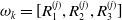 $\omega _k=[R_1^{(j)}, R_2^{(j)}, R_3^{(j)}]$
has the form
$\omega _k=[R_1^{(j)}, R_2^{(j)}, R_3^{(j)}]$
has the form
 \begin{equation} S \overset {R_1^{(j)}} \longrightarrow C_j \overset {R_2^{(j)}}\longrightarrow C_{j+1} \overset {R_3^{(j)}}\longrightarrow S. \end{equation}
A convenient way to measure the lack of detailed balance of the kinetic proofreading network is to introduce the parameter
 $\Delta _j$
, associated to each cycle
$\Delta _j$
, associated to each cycle
 $\omega _j$
, defined as
$\omega _j$
, defined as
 \begin{equation} e^{\Delta _{j} } \,:\!=\, \frac { k_{R_1^{(j)}}k_{R_2^{(j)}} k_{R_3^{(j)}} }{ k_{- R_1^{(j)} }k_{- R_2^{(j)} }k_{- R_3^{(j)} }}. \end{equation}
Notice that if
 $\Delta _{j} =0$
for every
$\Delta _{j} =0$
for every
 $j=1, \ldots , N$
, then the detailed balance property holds. We assume that every cycle has the same lack of detailed balance, i.e. for every
$j=1, \ldots , N$
, then the detailed balance property holds. We assume that every cycle has the same lack of detailed balance, i.e. for every
 $j$
it holds that
$j$
it holds that
 $\Delta _j= \Delta$
. We will use the parameter
$\Delta _j= \Delta$
. We will use the parameter
 $\Delta$
as a measure of the lack of detailed balance of the kinetic proofreading model. The parameter
$\Delta$
as a measure of the lack of detailed balance of the kinetic proofreading model. The parameter
 $\Delta$
is sometimes called thermodynamic force in the physics/chemistry literature (see [Reference Hill17]). In Section 3, we show that the amount of lack of detailed balance
$\Delta$
is sometimes called thermodynamic force in the physics/chemistry literature (see [Reference Hill17]). In Section 3, we show that the amount of lack of detailed balance
 $\Delta$
can be written in terms of external concentrations of ATP, ADP and phosphate groups, see equality (3.4).
$\Delta$
can be written in terms of external concentrations of ATP, ADP and phosphate groups, see equality (3.4).
The main results of this paper concern a kinetic proofreading model in which the property of detailed balance fails due to the fact that the phosphorylation reactions consume energy, i.e. consume ATP molecules and produce ADP molecules. This is modelled in this paper by assuming that the only chemical rates that depend on the parameter
 $\Delta$
are the chemical rates of the phosphorylation reactions
$\Delta$
are the chemical rates of the phosphorylation reactions
 $R_2^{(j)}$
, i.e. the chemical rates
$R_2^{(j)}$
, i.e. the chemical rates
 $k_{R_2^{(j)} }$
depend on
$k_{R_2^{(j)} }$
depend on
 $\Delta$
, while the rates
$\Delta$
, while the rates
 $ k_{R_1}^{(j)} ,k_{- R_1}^{(j)}, k_{-R_2^{(j)} }, k_{R_3}^{(j)}, k_{- R_3}^{(j)}$
are independent on
$ k_{R_1}^{(j)} ,k_{- R_1}^{(j)}, k_{-R_2^{(j)} }, k_{R_3}^{(j)}, k_{- R_3}^{(j)}$
are independent on
 $\Delta$
. We prove that this specific class of kinetic proofreading models exhibits strong discrimination properties if and only if
$\Delta$
. We prove that this specific class of kinetic proofreading models exhibits strong discrimination properties if and only if
 $\Delta \gt \Delta _c$
where
$\Delta \gt \Delta _c$
where
 $\Delta _c$
depends on the parameters of the model, i.e. on the phosphorylation rates, the energies of the substances in the network and the binding energy
$\Delta _c$
depends on the parameters of the model, i.e. on the phosphorylation rates, the energies of the substances in the network and the binding energy
 $\sigma$
of the ligand with the receptor.
$\sigma$
of the ligand with the receptor.
Since the value of
 $\Delta$
measures the lack of detailed balance (lack of equilibrium), one could naively think that this value could characterize the behaviour of the system even when we assume that the phosphorylation rates are independent on
$\Delta$
measures the lack of detailed balance (lack of equilibrium), one could naively think that this value could characterize the behaviour of the system even when we assume that the phosphorylation rates are independent on
 $ \Delta$
and the fact that equality (1.4) holds for
$ \Delta$
and the fact that equality (1.4) holds for
 $\Delta _j = \Delta \neq 0$
is due to the fact that either the detachment rates or the attachment rates depend on
$\Delta _j = \Delta \neq 0$
is due to the fact that either the detachment rates or the attachment rates depend on
 $\Delta$
. In other words, one could think that if the chemical rates
$\Delta$
. In other words, one could think that if the chemical rates
 $\{ k_{R_j } \}$
of the system (1.3) are such that (1.4) holds with
$\{ k_{R_j } \}$
of the system (1.3) are such that (1.4) holds with
 $\Delta _j = \Delta \gt \Delta _c$
, then the system satisfies strong discrimination properties.
$\Delta _j = \Delta \gt \Delta _c$
, then the system satisfies strong discrimination properties.
It turns out that this is not the case. In Section 8, we show that some choices of chemical rates
 $\{ k_{R_j } \}$
yielding lack of detailed balance, and specifically satisfying
$\{ k_{R_j } \}$
yielding lack of detailed balance, and specifically satisfying
 $\Delta \gt \Delta _c$
, produce strong discrimination properties while other choices of chemical rates, that give the same value of
$\Delta \gt \Delta _c$
, produce strong discrimination properties while other choices of chemical rates, that give the same value of
 $\Delta$
, do not. Specifically, in Section 8.1, we prove that if the only rates that depend on
$\Delta$
, do not. Specifically, in Section 8.1, we prove that if the only rates that depend on
 $\Delta$
are the detachment rates, then the system does not have strong specificity properties even if it satisfies (1.4) with
$\Delta$
are the detachment rates, then the system does not have strong specificity properties even if it satisfies (1.4) with
 $\Delta _j = \Delta \neq 0$
. Instead, in Section 8.2, we show that a model of kinetic proofreading with attachment rate depending on
$\Delta _j = \Delta \neq 0$
. Instead, in Section 8.2, we show that a model of kinetic proofreading with attachment rate depending on
 $\Delta$
satisfies the strong discrimination properties. Therefore, the fact that a network of the form (1.3) does not satisfy the detailed balance property is not a sufficient condition for strong specificity, even if
$\Delta$
satisfies the strong discrimination properties. Therefore, the fact that a network of the form (1.3) does not satisfy the detailed balance property is not a sufficient condition for strong specificity, even if
 $\Delta$
is very large. Indeed, it turns out that the details of the chemical reaction rates are also crucial and the fact that
$\Delta$
is very large. Indeed, it turns out that the details of the chemical reaction rates are also crucial and the fact that
 $\Delta \gt \Delta _c$
is a sufficient condition for strong specificity only for systems of the form (1.3) where the phosphorylation reaction rates
$\Delta \gt \Delta _c$
is a sufficient condition for strong specificity only for systems of the form (1.3) where the phosphorylation reaction rates
 $k_{R_2}^{(j) }$
depend on
$k_{R_2}^{(j) }$
depend on
 $\Delta$
.
$\Delta$
.
We already anticipated that we say that a chemical reaction network has strong discrimination properties if it can distinguish with low error rates ligands that are characterised by binding energies whose difference is of order
 $1/N$
. We clarify now what we mean by that in this paper. We prove that the characteristic time at which a complex ligand-receptor reaches the state
$1/N$
. We clarify now what we mean by that in this paper. We prove that the characteristic time at which a complex ligand-receptor reaches the state
 $C_{N}$
and therefore produces a response scales like
$C_{N}$
and therefore produces a response scales like
 \begin{equation*} T_N \sim \exp \left ( \lambda _\Delta (\sigma , E) N \right ) \text{ as } N \to \infty , \end{equation*}
where
 $\lambda _\Delta (\sigma , E)$
is a function of
$\lambda _\Delta (\sigma , E)$
is a function of
 $\sigma , E$
and
$\sigma , E$
and
 $\Delta$
. Suppose that the ligands and the receptors have a characteristic interaction time that satisfies
$\Delta$
. Suppose that the ligands and the receptors have a characteristic interaction time that satisfies
 \begin{equation} T_{signal} \sim \exp \left ( b N \right ) \text{ as } N \to \infty , \end{equation}
for a positive
 $b$
. Then, the probability
$b$
. Then, the probability
 $p_{res}(\sigma )$
that one ligand produces a response satisfies
$p_{res}(\sigma )$
that one ligand produces a response satisfies
 \begin{equation*} p_{res} (\sigma ) \sim \frac {e^{-\lambda _\Delta (\sigma , E) N}}{e^{-\lambda _\Delta (\sigma , E) N } + e^{-b N }} \text{ as } N \to \infty \end{equation*}
and will be close to
 $1$
when
$1$
when
 $ b - \lambda _\Delta (\sigma , E) \gtrsim 1/N$
and close to
$ b - \lambda _\Delta (\sigma , E) \gtrsim 1/N$
and close to
 $0$
when
$0$
when
 $ \lambda _\Delta (\sigma , E) - b \gtrsim 1/N$
.
$ \lambda _\Delta (\sigma , E) - b \gtrsim 1/N$
.
In this paper, we prove that for any binding energy
 $\sigma _c \in \mathbb R$
there exists a critical amount of detailed balance
$\sigma _c \in \mathbb R$
there exists a critical amount of detailed balance
 $\Delta _c(\sigma _c)$
that has the following property. If
$\Delta _c(\sigma _c)$
that has the following property. If
 $\Delta \gt \Delta _c(\sigma _c)$
, then we can find a parameter
$\Delta \gt \Delta _c(\sigma _c)$
, then we can find a parameter
 $b \in (0, E)$
such that
$b \in (0, E)$
such that
 $ \lambda _\Delta (\sigma _c, E) =b\lt E.$
Around the parameter
$ \lambda _\Delta (\sigma _c, E) =b\lt E.$
Around the parameter
 $\sigma _c$
, we have an abrupt transition from response to non-response. Indeed, if
$\sigma _c$
, we have an abrupt transition from response to non-response. Indeed, if
 $\sigma - \sigma _c \gtrsim \frac {1}{N}$
, we have that
$\sigma - \sigma _c \gtrsim \frac {1}{N}$
, we have that
 $p_{res} (\sigma ) \approx 0$
, while if
$p_{res} (\sigma ) \approx 0$
, while if
 $ \sigma _c - \sigma \gtrsim \frac {1}{N}$
, then
$ \sigma _c - \sigma \gtrsim \frac {1}{N}$
, then
 $p_{res} ( \sigma ) \approx 1$
. The region of transition from response to non-response, where we have that
$p_{res} ( \sigma ) \approx 1$
. The region of transition from response to non-response, where we have that
 $p_{res} ( \sigma ) \in (0,1)$
, is of order
$p_{res} ( \sigma ) \in (0,1)$
, is of order
 $1/N$
and is the region where we have
$1/N$
and is the region where we have
 \begin{equation*} | \sigma - \sigma _c | \lesssim \frac {1}{N} . \end{equation*}
Hence, the accuracy of the discrimination is of order
 $1/N$
. If instead we have that
$1/N$
. If instead we have that
 $\Delta \lt \Delta _c (\sigma _c)$
, it is not possible to find a
$\Delta \lt \Delta _c (\sigma _c)$
, it is not possible to find a
 $b$
such that
$b$
such that
 $\lambda _\Delta (\sigma _c , E) = b$
. Hence, in this case, we do not have a sharp transition from non response to response around a critical binding energy separating the energies leading to a response from the energies that do not lead to a response. In this case, the network does not have strong discrimination properties.
$\lambda _\Delta (\sigma _c , E) = b$
. Hence, in this case, we do not have a sharp transition from non response to response around a critical binding energy separating the energies leading to a response from the energies that do not lead to a response. In this case, the network does not have strong discrimination properties.
Notice that in this paper, we assume that
 $T_{signal}$
satisfies (1.5). However, also if
$T_{signal}$
satisfies (1.5). However, also if
 $ T_{signal} \lesssim N$
, it would be possible to study the discrimination properties of the kinetic proofreading model. Also in this case, we would have some discrimination properties, meaning that higher
$ T_{signal} \lesssim N$
, it would be possible to study the discrimination properties of the kinetic proofreading model. Also in this case, we would have some discrimination properties, meaning that higher
 $\sigma$
implies a smaller probability of response. However, in that setting, we would not obtain the existence of a sharp transition from
$\sigma$
implies a smaller probability of response. However, in that setting, we would not obtain the existence of a sharp transition from
 $1$
to
$1$
to
 $0$
for the probability of response around a critical value of
$0$
for the probability of response around a critical value of
 $\sigma$
.
$\sigma$
.
An interpretation of the critical behaviour found in this paper is the following. In the subcritical regime, the response is achieved by means of a direct jump from the signal
 $S$
to the final state
$S$
to the final state
 $C_N$
. Due to this fact, there is no dependence on
$C_N$
. Due to this fact, there is no dependence on
 $\sigma$
in the probability of response as
$\sigma$
in the probability of response as
 $N \to \infty$
. Instead, in the supercritical regime, the response is achieved through a transition of the system along the phosphorylation chain. In the second case, the process takes place faster due to the fact that
$N \to \infty$
. Instead, in the supercritical regime, the response is achieved through a transition of the system along the phosphorylation chain. In the second case, the process takes place faster due to the fact that
 $\lambda _\Delta (\sigma , E)$
is smaller than
$\lambda _\Delta (\sigma , E)$
is smaller than
 $E$
. Notice that the direct transition from
$E$
. Notice that the direct transition from
 $S$
to
$S$
to
 $N$
is very unlikely and is expected to take place in time scales of order
$N$
is very unlikely and is expected to take place in time scales of order
 $e^{EN}$
. However, in the supercritical regime, the process is faster and takes place at the time scale
$e^{EN}$
. However, in the supercritical regime, the process is faster and takes place at the time scale
 $e^{\lambda _\Delta (\sigma , E) N }$
, which is much shorter than
$e^{\lambda _\Delta (\sigma , E) N }$
, which is much shorter than
 $e^{EN}$
for
$e^{EN}$
for
 $N$
large.
$N$
large.
1.1. Notation
In this paper, we use the notation
 $\mathbb R_* = (0, \infty )$
and
$\mathbb R_* = (0, \infty )$
and
 $\mathbb N_0 = \mathbb N \setminus \{ 0\}$
. Moreover, we use the notation
$\mathbb N_0 = \mathbb N \setminus \{ 0\}$
. Moreover, we use the notation
 $ f \sim g$
as
$ f \sim g$
as
 $N \to \infty$
to indicate that the two functions
$N \to \infty$
to indicate that the two functions
 $f$
and
$f$
and
 $g$
are asymptotically equivalent, i.e.
$g$
are asymptotically equivalent, i.e.
 $\lim _{N \to \infty } \frac {f(N)}{g(N)} =1$
. We use the notation
$\lim _{N \to \infty } \frac {f(N)}{g(N)} =1$
. We use the notation
 $f \approx g$
to indicate that
$f \approx g$
to indicate that
 $f$
and
$f$
and
 $g$
are roughly of the same order. We say that
$g$
are roughly of the same order. We say that
 $f \gg g$
as
$f \gg g$
as
 $N \to \infty$
if it holds that
$N \to \infty$
if it holds that
 $\lim _{N \to \infty } \frac {g(N)}{f(N)}=0$
. Finally, we use
$\lim _{N \to \infty } \frac {g(N)}{f(N)}=0$
. Finally, we use
 $ f \gtrsim g$
to say that there exists a positive constant
$ f \gtrsim g$
to say that there exists a positive constant
 $c\gt 0$
such that
$c\gt 0$
such that
 $f \geq c g$
.
$f \geq c g$
.
2. Main result of the paper
In this section, we present the model that we study in this paper and the main results that we prove.
2.1. The model
We now explain the assumptions on the chemical rates that we make in this paper. The particular choice of parameters that we consider allows us to define a chemical reaction network in which
 $\Delta \geq 0$
measures the lack of detailed balance. To define the chemical reaction rates, we start associating to the states in the network a Gibbs free energy (that will be written in
$\Delta \geq 0$
measures the lack of detailed balance. To define the chemical reaction rates, we start associating to the states in the network a Gibbs free energy (that will be written in
 $k_B T$
units). Without loss of generality, we assume that the free energy
$k_B T$
units). Without loss of generality, we assume that the free energy
 $E_S$
of free ligands is the basal energy, and we normalize it to be equal to zero. We then assume that the energy difference produced by each phosphorylation event is
$E_S$
of free ligands is the basal energy, and we normalize it to be equal to zero. We then assume that the energy difference produced by each phosphorylation event is
 $E \gt 0$
. We denote with
$E \gt 0$
. We denote with
 $\sigma \in \mathbb R$
the binding energy between the receptor and the ligand. This allows us to assume that the Gibbs free energy associated to a complex ligand-receptor at phosphorylation state
$\sigma \in \mathbb R$
the binding energy between the receptor and the ligand. This allows us to assume that the Gibbs free energy associated to a complex ligand-receptor at phosphorylation state
 $j \in \{ 0, \ldots , N \}$
(i.e. a complex ligand receptor with attached
$j \in \{ 0, \ldots , N \}$
(i.e. a complex ligand receptor with attached
 $j$
phosphate groups) is
$j$
phosphate groups) is
 $E_j \,:\!=\, \sigma + j E$
.
$E_j \,:\!=\, \sigma + j E$
.
As we will explain below, the assumptions we made on the Gibbs free energies allow us to write the chemical rates associated to the chemical reactions as follows. We assume that the attachment of a ligand to the receptor, i.e. the reactions of the form
 \begin{equation*} {R_1^{(j)} \,:\, S \overset {e^{ -j E } }{\longrightarrow } C_j} \end{equation*}
take place at rate
 $k_{R_1^{(j)}} =e^{- j E }$
for every
$k_{R_1^{(j)}} =e^{- j E }$
for every
 $j \in \{ 0, \ldots , N \}$
. The detachment rate depends on the binding energy between the ligand and the receptor, i.e. the reactions of the form
$j \in \{ 0, \ldots , N \}$
. The detachment rate depends on the binding energy between the ligand and the receptor, i.e. the reactions of the form
 \begin{equation*} {-R_1^{(j)}\,:\, C_{j} \overset {e^{\sigma } }{\longrightarrow } S } \end{equation*}
take place at rate
 $k_{- R_1^{(j)}} = e^{\sigma }$
for every
$k_{- R_1^{(j)}} = e^{\sigma }$
for every
 $j \in \{0, \ldots , N \}$
where
$j \in \{0, \ldots , N \}$
where
 $\sigma \in \mathbb R$
. The reactions
$\sigma \in \mathbb R$
. The reactions
 \begin{equation*} {R^{(j)}_2\,:\, C_j \overset {\alpha e^\Delta }{\longrightarrow } C_{j+1} } \end{equation*}
take place at rate
 $k_{R_2^{(j)}}= \alpha e^{\Delta }$
for every
$k_{R_2^{(j)}}= \alpha e^{\Delta }$
for every
 $j \in \{ 0, \ldots , N \}$
. On the other hand, we assume that the reaction
$j \in \{ 0, \ldots , N \}$
. On the other hand, we assume that the reaction
 \begin{equation*} {-R^{(j)}_2\,:\, C_j \overset {\alpha e^{E } }{\longrightarrow } C_{j-1} } \end{equation*}
takes place at rate
 $k_{-R^{(j)}_2}=\alpha e^{E_j- E_{j-1} }= \alpha e^E$
for every
$k_{-R^{(j)}_2}=\alpha e^{E_j- E_{j-1} }= \alpha e^E$
for every
 $j \in \{0, \ldots , N \}$
.
$j \in \{0, \ldots , N \}$
.
This is the sketch of the chemical reactions considered in this paper and the corresponding chemical rates.

See Figure 1 for a visual representation of the model. We now explain our choice of chemical rates and their interpretation. To this end, it is convenient to assume that
 $\Delta =0$
and that
$\Delta =0$
and that
 $b =0$
. Indeed, when
$b =0$
. Indeed, when
 $\Delta =0$
, we have that
$\Delta =0$
, we have that
 \begin{equation*} 1= \frac { k_{R_1^{(j)}}k_{R_2^{(j)}} k_{-R_1^{(j+1)}} }{ k_{- R_1^{(j)} }k_{- R_2^{(j)} }k_{ R_1^{(j +1)} }} \end{equation*}
for every cycle
 \begin{equation*} S \overset {R_1^{(j)}} \longrightarrow C_j \overset {R_2^{(j)}}\longrightarrow C_{j+1} \overset {- R_1^{(+1)}}\longrightarrow S. \end{equation*}
The Wegscheider criterium then guarantees that detailed balance holds when
 $\Delta =0$
. It is well known that in this case the ratio between the chemical rate of the direct reaction and the chemical rate of the reverse reaction can be written in terms of the Gibbs free energies. More precisely, for the specific system under consideration, we have that
$\Delta =0$
. It is well known that in this case the ratio between the chemical rate of the direct reaction and the chemical rate of the reverse reaction can be written in terms of the Gibbs free energies. More precisely, for the specific system under consideration, we have that
 \begin{equation} \frac {k_{R_1^{(j)}} }{k_{- R_1^{(j)}}} = e^{ - E_j } , \quad \frac {k_{R_2^{(j)}} }{k_{- R_2^{(j)}}} = e^{ E_{j} - E_{j+1} } =e^{-E} , \quad j \in \{ 0, \ldots , N \}. \end{equation}
Notice that our choice of chemical rates satisfies (2.1) when
 $\Delta =0$
. The parameter
$\Delta =0$
. The parameter
 $\alpha$
is the constant of proportionality between
$\alpha$
is the constant of proportionality between
 $k_{ R_2^{(j)}}$
and
$k_{ R_2^{(j)}}$
and
 $k_{- R_2^{(j)}} e^{ E_j - E_{j+1} }$
. Finally, since we want to study a system with lack of detailed balance and since we assume that the energy is consumed during the phosphorylation reactions
$k_{- R_2^{(j)}} e^{ E_j - E_{j+1} }$
. Finally, since we want to study a system with lack of detailed balance and since we assume that the energy is consumed during the phosphorylation reactions
 $R_2^{\kern1pt j}$
, we define the chemical rates
$R_2^{\kern1pt j}$
, we define the chemical rates
 $k_{R_2}^{(j) }$
as
$k_{R_2}^{(j) }$
as
 $e^\Delta k^{DB}_{{R_2}^{(j)}}$
, where
$e^\Delta k^{DB}_{{R_2}^{(j)}}$
, where
 $ k^{DB}_{{R_2}^{(j)}}$
is the rate of the phosphorylation reaction when detailed balance holds, hence
$ k^{DB}_{{R_2}^{(j)}}$
is the rate of the phosphorylation reaction when detailed balance holds, hence
 $ k^{DB}_{{R_2}^{(j)}} =\alpha$
.
$ k^{DB}_{{R_2}^{(j)}} =\alpha$
.
We call the parameter
 $\sigma$
that determines the detachment rate, binding energy because it is the energy associated with the dephosphorylated complex ligand-receptor
$\sigma$
that determines the detachment rate, binding energy because it is the energy associated with the dephosphorylated complex ligand-receptor
 $C_0$
. In the chemical literature, the detachment rate is usually written as
$C_0$
. In the chemical literature, the detachment rate is usually written as
 $ e^{ - E_A}$
where
$ e^{ - E_A}$
where
 $E_A$
is the activation energy of the unbinding reaction. Due to the normalization
$E_A$
is the activation energy of the unbinding reaction. Due to the normalization
 $E_S =0$
that we make in our model and the assumption that the rate of the reaction
$E_S =0$
that we make in our model and the assumption that the rate of the reaction
 $S \rightarrow C_0$
is equal to
$S \rightarrow C_0$
is equal to
 $1$
, it turns out that, for the specific model under consideration, the energy
$1$
, it turns out that, for the specific model under consideration, the energy
 $\sigma$
completely determines the detachment rate, which is
$\sigma$
completely determines the detachment rate, which is
 $e^\sigma$
.
$e^\sigma$
.
The assumptions above on the chemical rates guarantee that for every cycle
 $\omega _k=[R_1^{(j)}, R_2^{(j)}, -R_1^{(j+1)}]$
of the form
$\omega _k=[R_1^{(j)}, R_2^{(j)}, -R_1^{(j+1)}]$
of the form
 \begin{equation*} S \overset {R_1^{(j)}} \longrightarrow C_j \overset {R_2^{(j)}}\longrightarrow C_{j+1} \overset {- R_1^{(j+1)}}\longrightarrow S \end{equation*}
it holds that
 \begin{equation} {e^{\Delta } = \frac { k_{R_1^{(j)}}k_{R_2^{(j)}} k_{-R_1^{(j+1)}} }{ k_{- R_1^{(j)} }k_{- R_2^{(j)} }k_{ R_1^{(j +1)} }}. } \end{equation}
Hence, when
 $\Delta \neq 0$
, the detailed balance property does not hold. We stress that we are assuming here that the only reactions that are affected by the parameter
$\Delta \neq 0$
, the detailed balance property does not hold. We stress that we are assuming here that the only reactions that are affected by the parameter
 $\Delta$
are the phosphorylation reactions
$\Delta$
are the phosphorylation reactions
 $C_j \rightarrow C_{j+1}$
. The fact that detailed balance fails along these reactions implies that the rate
$C_j \rightarrow C_{j+1}$
. The fact that detailed balance fails along these reactions implies that the rate
 $\alpha e^\Delta$
of the phosphorylation reactions is larger than the rate that we have when detailed balance holds, i.e.
$\alpha e^\Delta$
of the phosphorylation reactions is larger than the rate that we have when detailed balance holds, i.e.
 $\alpha$
. In other words, the lack of detailed balance accelerates the phosphorylation reactions.
$\alpha$
. In other words, the lack of detailed balance accelerates the phosphorylation reactions.
Finally, we assume that the ligand can jump to the absorbing state
 $\emptyset$
from any other state. Once the ligand reaches the absorbing state
$\emptyset$
from any other state. Once the ligand reaches the absorbing state
 $\emptyset$
, it cannot interact again with the receptor. The rationale behind this is that we assume that the pMHC and the T-cells interact for a characteristic time that we call signalling lifetime, and we denote with
$\emptyset$
, it cannot interact again with the receptor. The rationale behind this is that we assume that the pMHC and the T-cells interact for a characteristic time that we call signalling lifetime, and we denote with
 $\mu ^{-1}$
. We stress that the fact that the ligand reaches the state
$\mu ^{-1}$
. We stress that the fact that the ligand reaches the state
 $\emptyset$
does not necessarily mean that the ligand is degraded. The ligand can reach the state
$\emptyset$
does not necessarily mean that the ligand is degraded. The ligand can reach the state
 $\emptyset$
also, for instance, due to the fact that the pMHC stops interacting with the T-cells or due to the fact that the activation time of the receptors is limited due to any kind of mechanism, including ligand degradation, T-cell motion, or the detachment of the peptide from the MHC.
$\emptyset$
also, for instance, due to the fact that the pMHC stops interacting with the T-cells or due to the fact that the activation time of the receptors is limited due to any kind of mechanism, including ligand degradation, T-cell motion, or the detachment of the peptide from the MHC.
The existence of a characteristic interaction time between the ligands and the receptors is crucial in kinetic proofreading systems. If we assume that the interaction time between the T-cells and ligands is unbounded (and hence
 $\mu =0$
), then all the ligands will eventually produce a response, even if the response would require a very long time. Therefore, the strong specificity property cannot hold when
$\mu =0$
), then all the ligands will eventually produce a response, even if the response would require a very long time. Therefore, the strong specificity property cannot hold when
 $\mu =0$
.
$\mu =0$
.
Moreover, we assume that the signalling lifetime
 $\mu ^{-1}$
is such that
$\mu ^{-1}$
is such that
 \begin{equation} \mu \sim e^{- b N } \text{ as } N \to \infty \end{equation}
where
 $b \gt 0$
. This means that the characteristic time at which the interaction between the T-cells and the ligands takes place scales as
$b \gt 0$
. This means that the characteristic time at which the interaction between the T-cells and the ligands takes place scales as
 $T \sim e^{bN }$
as
$T \sim e^{bN }$
as
 $N \to \infty$
. This is a mathematical assumption that we make to get a precise scaling limit in which we can prove that strong specificity properties hold. We do not claim that there exists a physical dependence between the characteristic interaction time and the number of kinetic proofreading steps, but the numerical relation between
$N \to \infty$
. This is a mathematical assumption that we make to get a precise scaling limit in which we can prove that strong specificity properties hold. We do not claim that there exists a physical dependence between the characteristic interaction time and the number of kinetic proofreading steps, but the numerical relation between
 $\mu$
and
$\mu$
and
 $N$
allows to obtain a mathematical limit in which the strong specificity property can be defined in precise mathematical terms.
$N$
allows to obtain a mathematical limit in which the strong specificity property can be defined in precise mathematical terms.
Let
 $n_k (t)$
be the probability that a ligand, characterised by the binding energy
$n_k (t)$
be the probability that a ligand, characterised by the binding energy
 $\sigma$
, reaches the state
$\sigma$
, reaches the state
 $k \in \{ 0, \ldots , N\}$
in the time interval
$k \in \{ 0, \ldots , N\}$
in the time interval
 $(0, t ]$
and let
$(0, t ]$
and let
 $n_S (t)$
be the probability that it reaches the state
$n_S (t)$
be the probability that it reaches the state
 $S$
in the time interval
$S$
in the time interval
 $(0, t ]$
. The dynamics of the vector of the probabilities
$(0, t ]$
. The dynamics of the vector of the probabilities
 $n(t)=(n_S(t), n_0(t), n_1(t), \ldots , n_N(t) )^T \in \mathbb R_*^{N+1}$
is described by the following system of ODEs
$n(t)=(n_S(t), n_0(t), n_1(t), \ldots , n_N(t) )^T \in \mathbb R_*^{N+1}$
is described by the following system of ODEs

with initial datum
 $n(0)=(1, 0, \ldots , 0)$
and where
$n(0)=(1, 0, \ldots , 0)$
and where
 \begin{equation*} S_N(E)\,:\!=\,\sum _{k=1}^{N} e^{- k E } = \frac {1-e^{-NE}}{e^E-1 } . \end{equation*}
The fact that we are considering as initial datum
 $n(0)=(1, 0, \ldots , 0)$
means that at time
$n(0)=(1, 0, \ldots , 0)$
means that at time
 $t=0$
the only substances present in the network are the free ligands. The probability that a ligand, characterized by the binding energy
$t=0$
the only substances present in the network are the free ligands. The probability that a ligand, characterized by the binding energy
 $\sigma$
, produces a response in the time interval
$\sigma$
, produces a response in the time interval
 $(0,t]$
, denoted with
$(0,t]$
, denoted with
 $R(t)$
, is given by
$R(t)$
, is given by
 \begin{equation*} {R(t) \,:\!=\, \alpha e^\Delta \int _0^t n_N(s ) ds .} \end{equation*}
The probability
 $p_{deg} (t)$
that a ligand stops interacting with the receptor before producing a response in the time interval
$p_{deg} (t)$
that a ligand stops interacting with the receptor before producing a response in the time interval
 $(0, t]$
is defined as
$(0, t]$
is defined as
 \begin{equation*} {p_{deg} (t) \,:\!=\, \mu \int _0^t M(s) ds } \end{equation*}
where
 $M(t)$
can be interpreted as the probability that the ligand is in the network (either in a complex or as a free ligand) in the time interval
$M(t)$
can be interpreted as the probability that the ligand is in the network (either in a complex or as a free ligand) in the time interval
 $(0, t]$
 \begin{equation} M(t)\,:\!=\,n_S(t) +\sum _{k=0}^{N} n_k (t) . \end{equation}
Later, we refer to
 $M$
as the total mass of ligands in the network. According to the system of equations introduced above, we have that
$M$
as the total mass of ligands in the network. According to the system of equations introduced above, we have that
 $M$
is decreasing in time. More precisely, we have that
$M$
is decreasing in time. More precisely, we have that
 \begin{equation} \frac {d M }{ dt } = - \alpha e^\Delta n_{N} - \mu M . \end{equation}
Finally, notice that, as expected, we have that
 \begin{equation*} p_{deg}(t) + R(t) + M(t)=1, \quad \forall t \geq 0. \end{equation*}
In this paper, we analyse the probability
 $p_{res}(\sigma )$
that one ligand characterised by its binding energy
$p_{res}(\sigma )$
that one ligand characterised by its binding energy
 $\sigma$
with the receptor produce a responses, i.e.
$\sigma$
with the receptor produce a responses, i.e.
 \begin{equation} p_{res} (\sigma ) \,:\!=\, \int _0^\infty R(t) dt = \alpha e^\Delta \int _0^\infty n_{N} (t) dt \end{equation}
as the number of kinetic proofreading steps
 $N \to \infty$
. In other words,
$N \to \infty$
. In other words,
 $p_{res} (\sigma )$
is the probability that the lifetime of the ligand is longer than the time to reach the phosphorylation state
$p_{res} (\sigma )$
is the probability that the lifetime of the ligand is longer than the time to reach the phosphorylation state
 $C_N$
(when both times are exponentially distributed).
$C_N$
(when both times are exponentially distributed).
2.2. Strong discrimination properties for
 $\Delta \gt \Delta _c$

The goal of the paper is to analyse the relation between the lack of detailed balance and strong discrimination properties of kinetic proofreading mechanisms. We state here precisely our definition of strong discrimination.
Definition 2.1 (Strong discrimination). Let
 $\Delta , \sigma , b, E , \alpha$
be positive constants. The kinetic proofreading network described by the system of ODEs (2.4) has strong discrimination properties with respect to the energy
$\Delta , \sigma , b, E , \alpha$
be positive constants. The kinetic proofreading network described by the system of ODEs (2.4) has strong discrimination properties with respect to the energy
 $\sigma$
if
$\sigma$
if
 \begin{equation} \lim _{N \to \infty } \frac {1}{N } \log \left ( \frac {1}{p_{res} (\sigma ) } - 1 \right ) = \lambda _\Delta (\sigma , E) - b \end{equation}
where
 $ \lambda _\Delta (\sigma , E )$
is a parameter that depends non trivially on
$ \lambda _\Delta (\sigma , E )$
is a parameter that depends non trivially on
 $\sigma$
and there exists a solution
$\sigma$
and there exists a solution
 $\sigma _c$
to
$\sigma _c$
to
 \begin{equation} \lambda _\Delta (\sigma _c, E)= b. \end{equation}
We recall that the parameter
 $b$
here characterizes the ligand signalling lifetime as the number of kinetic proofreading steps
$b$
here characterizes the ligand signalling lifetime as the number of kinetic proofreading steps
 $N$
goes to infinity (see 2.3).
$N$
goes to infinity (see 2.3).
In this paper, we prove that for the kinetic proofreading networks introduced in Section 2.1, we have that the probability of response always satisfies (2.8), but
 $\lambda _\Delta (\sigma , E)$
depends non trivially on
$\lambda _\Delta (\sigma , E)$
depends non trivially on
 $\sigma$
only when
$\sigma$
only when
 $\Delta \gt \Delta _c(\sigma )$
; indeed, we will prove that
$\Delta \gt \Delta _c(\sigma )$
; indeed, we will prove that
 \begin{equation} \lambda _\Delta (\sigma , E )=\begin{cases} E &\text{ if } \Delta \lt \Delta _c (\sigma ) \\ \psi _\Delta (\sigma , E) &\text{ if } \Delta \gt \Delta _c(\sigma ) \end{cases} \end{equation}
where
 $\psi$
is a function which depends non trivially on
$\psi$
is a function which depends non trivially on
 $\sigma$
,
$\sigma$
,
 $E$
and
$E$
and
 $\Delta$
 \begin{equation} \psi _\Delta (\sigma , E ) \,:\!=\, E - \log \left [ \frac {1}{2 \alpha } \left ( e^\sigma + \alpha (e^E+ e^\Delta ) - \sqrt { (e^\sigma + \alpha (e^E+ e^\Delta ) )^2 - 4 \alpha ^2 e^{\Delta + E }} \right ) \right ] \end{equation}
and where
 \begin{equation} \Delta _c= \Delta _c (\sigma ) \,:\!=\, \log \left ( 1+ \frac {e^\sigma }{\alpha (e^E-1 ) } \right ). \end{equation}
In the latter, for notational convenience, we will remove the subscript
 $\Delta$
from
$\Delta$
from
 $\lambda _\Delta$
and from
$\lambda _\Delta$
and from
 $\psi _\Delta$
.
$\psi _\Delta$
.
The fact that
 $\lambda (\sigma , E)$
does not depend on
$\lambda (\sigma , E)$
does not depend on
 $\sigma$
for
$\sigma$
for
 $\Delta$
and
$\Delta$
and
 $\sigma$
such that
$\sigma$
such that
 $\Delta \lt \Delta _c(\sigma )$
and depends on
$\Delta \lt \Delta _c(\sigma )$
and depends on
 $\sigma$
for
$\sigma$
for
 $\Delta$
and
$\Delta$
and
 $\sigma$
such that
$\sigma$
such that
 $\Delta \gt \Delta _c(\sigma )$
is the most important result of this paper. It implies that the kinetic proofreading networks described by (2.4) can have strong discrimination properties, in the sense of Definition 2.1, only when
$\Delta \gt \Delta _c(\sigma )$
is the most important result of this paper. It implies that the kinetic proofreading networks described by (2.4) can have strong discrimination properties, in the sense of Definition 2.1, only when
 $\Delta$
and
$\Delta$
and
 $\sigma$
are such that
$\sigma$
are such that
 $\Delta \gt \Delta _c(\sigma )$
.
$\Delta \gt \Delta _c(\sigma )$
.
2.3. Necessary conditions on
$b$
for strong discrimination when
$\Delta \gt \Delta _c$


The goal of this section is to explain how to interpret the consequences of the definition of strong discrimination given in Section 4.3 and in particular to introduce a condition on the parameter
 $b$
that is necessary in order to have that equation (2.9) admits a solution, hence that the strong discrimination property holds.
$b$
that is necessary in order to have that equation (2.9) admits a solution, hence that the strong discrimination property holds.
The fact that the parameter
 $\lambda (\sigma , E)$
depends on
$\lambda (\sigma , E)$
depends on
 $\sigma$
is crucial in order to have a sharp transition of
$\sigma$
is crucial in order to have a sharp transition of
 $p_{res} (\sigma )$
from
$p_{res} (\sigma )$
from
 $1$
to
$1$
to
 $0$
around a critical binding energy
$0$
around a critical binding energy
 $\sigma _c$
. Indeed, (2.8) implies that the probability
$\sigma _c$
. Indeed, (2.8) implies that the probability
 $p_{res} (\sigma )$
that one ligand characterized by the binding energy
$p_{res} (\sigma )$
that one ligand characterized by the binding energy
 $\sigma$
satisfies
$\sigma$
satisfies
 \begin{equation} p_{res} (\sigma ) \sim \left ( 1 + Ce^{N(\lambda (\sigma , E)- b)}\right )^{-1} \text{ as } N \to \infty \end{equation}
where
 $C$
is a positive constant that depends on the parameters. When
$C$
is a positive constant that depends on the parameters. When
 $\Delta \lt \Delta _c(\sigma )$
, we have that
$\Delta \lt \Delta _c(\sigma )$
, we have that
 $\lambda (\sigma , E )=E$
. As a consequence, if
$\lambda (\sigma , E )=E$
. As a consequence, if
 $\lambda (\sigma , E )=E \lt b$
, then
$\lambda (\sigma , E )=E \lt b$
, then
 $\lim _{N\to \infty } p_{res} (\sigma ) =1$
, while when
$\lim _{N\to \infty } p_{res} (\sigma ) =1$
, while when
 $\lambda (\sigma , E )=E \gt b$
, then
$\lambda (\sigma , E )=E \gt b$
, then
 $\lim _{N\to \infty } p_{res} (\sigma ) =0$
. As will be explained in detail in Section 8.4, when
$\lim _{N\to \infty } p_{res} (\sigma ) =0$
. As will be explained in detail in Section 8.4, when
 $\Delta \to \infty$
and
$\Delta \to \infty$
and
 $\alpha , E , \sigma$
are of order one, the function
$\alpha , E , \sigma$
are of order one, the function
 $\psi$
does not depend on
$\psi$
does not depend on
 $ \sigma$
and we have a similar behaviour. The model in this case does not have strong discrimination properties in the sense of Definition 2.1.
$ \sigma$
and we have a similar behaviour. The model in this case does not have strong discrimination properties in the sense of Definition 2.1.
Consider a binding energy
 $ \sigma _c \in \mathbb R$
. Assume that
$ \sigma _c \in \mathbb R$
. Assume that
 $\Delta \gt \Delta _c = \Delta _c( \sigma _c)$
. By the continuity of the function
$\Delta \gt \Delta _c = \Delta _c( \sigma _c)$
. By the continuity of the function
 $\Delta _c(\sigma )$
defined by (2.12), there exists a neighbourhood
$\Delta _c(\sigma )$
defined by (2.12), there exists a neighbourhood
 $U$
of
$U$
of
 $\sigma _c$
such that
$\sigma _c$
such that
 $\lambda (\sigma , E )$
is a strictly increasing function of
$\lambda (\sigma , E )$
is a strictly increasing function of
 $\sigma$
in
$\sigma$
in
 $U$
. Then, we can find a parameter
$U$
. Then, we can find a parameter
 $b\gt 0$
such that (2.9) holds. Precise conditions that the parameter
$b\gt 0$
such that (2.9) holds. Precise conditions that the parameter
 $b$
must satisfy are given in (4.28). In particular, we must have that
$b$
must satisfy are given in (4.28). In particular, we must have that
 $b\lt E$
. The reason is that
$b\lt E$
. The reason is that
 $\lambda (\sigma _c, E)=\psi (\sigma _c, E)$
is a decreasing function of
$\lambda (\sigma _c, E)=\psi (\sigma _c, E)$
is a decreasing function of
 $\Delta$
. Therefore, in order to have that
$\Delta$
. Therefore, in order to have that
 $(\sigma _c, \Delta )$
are in the region of strong discrimination in Figure 2, we must have
$(\sigma _c, \Delta )$
are in the region of strong discrimination in Figure 2, we must have
 $\psi (\sigma _c, E ) = b \lt E$
.
$\psi (\sigma _c, E ) = b \lt E$
.
In this figure, we plot the line
 $\psi (\sigma , E)=E$
for
$\psi (\sigma , E)=E$
for
 $\alpha =1$
,
$\alpha =1$
,
 $E=\ln (2)$
. Notice that
$E=\ln (2)$
. Notice that
 $\psi (\sigma , E )=E$
if and only if
$\psi (\sigma , E )=E$
if and only if
 $\Delta = \Delta _c(\sigma )$
. The line
$\Delta = \Delta _c(\sigma )$
. The line
 $\psi (\sigma , E)=E$
separates the region in which we have strong discrimination properties from the region where we do not have strong discrimination.
$\psi (\sigma , E)=E$
separates the region in which we have strong discrimination properties from the region where we do not have strong discrimination.

The condition
 $b \lt E$
, needed to have strong discrimination, has an interpretation: the characteristic lifetime of the ligands
$b \lt E$
, needed to have strong discrimination, has an interpretation: the characteristic lifetime of the ligands
 $e^{bN}$
must be strictly smaller than the characteristic time to reach the state
$e^{bN}$
must be strictly smaller than the characteristic time to reach the state
 $N$
directly from the signal
$N$
directly from the signal
 $S$
, i.e.
$S$
, i.e.
 $e^{EN}$
as
$e^{EN}$
as
 $N \to \infty$
.
$N \to \infty$
.
The fact that there exists a
 $\sigma _c$
such that (2.9) holds implies that there exists a region of transition from response (
$\sigma _c$
such that (2.9) holds implies that there exists a region of transition from response (
 $p_{res}(\sigma ) =1$
) to non-response (
$p_{res}(\sigma ) =1$
) to non-response (
 $p_{res}(\sigma ) =0$
) when
$p_{res}(\sigma ) =0$
) when
 $\sigma$
is such that
$\sigma$
is such that
 \begin{equation*} |\lambda (\sigma , E ) - \lambda (\sigma _c, E ) |= |\lambda (\sigma , E) -b | \lesssim \frac {1}{N}. \end{equation*}
Moreover, we have that if
 $\sigma \gt \sigma _c$
is such that
$\sigma \gt \sigma _c$
is such that
 $ | \lambda (\sigma , E) - \lambda (\sigma _c, E) | \gtrsim \frac {1}{N}$
, then
$ | \lambda (\sigma , E) - \lambda (\sigma _c, E) | \gtrsim \frac {1}{N}$
, then
 $\lim _{N\to \infty } p_{res} (\sigma ) =0$
while when
$\lim _{N\to \infty } p_{res} (\sigma ) =0$
while when
 $\sigma \lt \sigma _c$
is such that
$\sigma \lt \sigma _c$
is such that
 $| \lambda (\sigma _c , E) - \lambda (\sigma , E ) | \gtrsim \frac {1}{N}$
, then
$| \lambda (\sigma _c , E) - \lambda (\sigma , E ) | \gtrsim \frac {1}{N}$
, then
 $\lim _{N\to \infty } p_{res} (\sigma ) =1$
.
$\lim _{N\to \infty } p_{res} (\sigma ) =1$
.
In Definition 2.1, we say that the kinetic proofreading model has strong discrimination properties if
 $\lambda (\sigma , E)$
depends on
$\lambda (\sigma , E)$
depends on
 $\sigma$
and when there exists a solution to (2.9), because in this case there exists a critical binding energy
$\sigma$
and when there exists a solution to (2.9), because in this case there exists a critical binding energy
 $\sigma _c$
which separates the binding energies that produce response from the binding energies that do not produce a response. Moreover, the size of the region of transition from response to non-response, in the space of binding energies
$\sigma _c$
which separates the binding energies that produce response from the binding energies that do not produce a response. Moreover, the size of the region of transition from response to non-response, in the space of binding energies
 $\sigma$
, where errors in the detection of ligands can occur, is of order
$\sigma$
, where errors in the detection of ligands can occur, is of order
 $1/N$
, hence tends to zero as
$1/N$
, hence tends to zero as
 $N \to \infty$
. In Figure 5, we compare the probability of response
$N \to \infty$
. In Figure 5, we compare the probability of response
 $p_{res} (\sigma )$
that we obtain selecting the parameters in such a way that
$p_{res} (\sigma )$
that we obtain selecting the parameters in such a way that
 $\Delta \gt \Delta _c$
with the probability of response when
$\Delta \gt \Delta _c$
with the probability of response when
 $\Delta \lt \Delta _c$
. Notice that in the latter case, the probability is almost constantly equal to
$\Delta \lt \Delta _c$
. Notice that in the latter case, the probability is almost constantly equal to
 $0$
, while in the first case, we have a sharp transition from response to non response around a critical binding energy
$0$
, while in the first case, we have a sharp transition from response to non response around a critical binding energy
 $\sigma _c$
.
$\sigma _c$
.
Due to the fact that
 $\Delta _c(\sigma ) \rightarrow 0$
as
$\Delta _c(\sigma ) \rightarrow 0$
as
 $ \sigma \to - \infty$
, it is not possible to prove the existence of a minimal lack of detailed balance in order to have strong specificity for all the binding energies
$ \sigma \to - \infty$
, it is not possible to prove the existence of a minimal lack of detailed balance in order to have strong specificity for all the binding energies
 $\sigma$
. However, it is possible to define a critical lack of detailed balance
$\sigma$
. However, it is possible to define a critical lack of detailed balance
 $\overline \Delta _c$
if the order of magnitude of
$\overline \Delta _c$
if the order of magnitude of
 $\sigma$
is prescribed. More precisely, suppose that we want to study the ability of a kinetic system to distinguish between ligands characterized by binding energies that are in the interval
$\sigma$
is prescribed. More precisely, suppose that we want to study the ability of a kinetic system to distinguish between ligands characterized by binding energies that are in the interval
 $I\,:\!=\, [\sigma _m , \sigma _M ]$
. Let us define
$I\,:\!=\, [\sigma _m , \sigma _M ]$
. Let us define
 $\overline \Delta _c \,:\!=\, \max _{\sigma \in I } \Delta _c(\sigma )$
. If
$\overline \Delta _c \,:\!=\, \max _{\sigma \in I } \Delta _c(\sigma )$
. If
 $\Delta \gt \overline \Delta _c$
, then (2.10) implies that
$\Delta \gt \overline \Delta _c$
, then (2.10) implies that
 $\lambda _\Delta (\sigma , E)$
depends non trivially on
$\lambda _\Delta (\sigma , E)$
depends non trivially on
 $\sigma$
on the interval
$\sigma$
on the interval
 $ I$
. Assume that
$ I$
. Assume that
 $b= \lambda _\Delta (\sigma _c, E )$
for some
$b= \lambda _\Delta (\sigma _c, E )$
for some
 $\sigma _c \in I$
. As a consequence, since
$\sigma _c \in I$
. As a consequence, since
 $p_{res}(\sigma )$
satisfies (2.8), we deduce that if
$p_{res}(\sigma )$
satisfies (2.8), we deduce that if
 $\Delta \gt \overline \Delta _c$
then the strong discrimination property holds. In particular, we will see a sharp transition from
$\Delta \gt \overline \Delta _c$
then the strong discrimination property holds. In particular, we will see a sharp transition from
 $1$
to
$1$
to
 $0$
in the probability of transition
$0$
in the probability of transition
 $p_{res} (\sigma )$
in region of order
$p_{res} (\sigma )$
in region of order
 $1/N$
around the critical binding energy
$1/N$
around the critical binding energy
 $\sigma _c$
.
$\sigma _c$
.
If, instead, we define
 $ \underline { \Delta _c} \,:\!=\, \min _{\sigma \in I } \Delta _c(\sigma )$
and consider
$ \underline { \Delta _c} \,:\!=\, \min _{\sigma \in I } \Delta _c(\sigma )$
and consider
 $\Delta \lt \underline { \Delta _c}$
, then the system does not have strong discrimination properties as
$\Delta \lt \underline { \Delta _c}$
, then the system does not have strong discrimination properties as
 $\lambda _\Delta (\sigma , E)= E$
for every
$\lambda _\Delta (\sigma , E)= E$
for every
 $\sigma \in I$
. Hence, depending on whether
$\sigma \in I$
. Hence, depending on whether
 $b \gt E$
or
$b \gt E$
or
 $E \gt b$
, we will have either that
$E \gt b$
, we will have either that
 $p_{res}(\sigma ) \approx 1$
for every
$p_{res}(\sigma ) \approx 1$
for every
 $\sigma \in I$
or that
$\sigma \in I$
or that
 $p_{res}(\sigma ) \approx 0$
for every
$p_{res}(\sigma ) \approx 0$
for every
 $\sigma \in I$
.
$\sigma \in I$
.
Finally, let us consider the limiting case in which
 $\Delta \to \infty$
and
$\Delta \to \infty$
and
 $\alpha , \sigma$
, and
$\alpha , \sigma$
, and
 $E$
are of order one. Under these assumptions, we have that
$E$
are of order one. Under these assumptions, we have that
 \begin{equation*} \lim _{\Delta \to \infty } \psi (\sigma , E )= E. \end{equation*}
Therefore, in this regime
 $\psi (\sigma , E)$
does not depend on
$\psi (\sigma , E)$
does not depend on
 $\sigma$
, hence we do not have strong discrimination properties. More details on the limiting cases with
$\sigma$
, hence we do not have strong discrimination properties. More details on the limiting cases with
 $\Delta \to \infty$
will be presented in Section 8.
$\Delta \to \infty$
will be presented in Section 8.
2.4. Some numerical solutions
In Figure 3, we compare the probability of response that we compute numerically when
 $N=3$
and when the lack of detailed balance is very small with the probability of response that we compute numerically for
$N=3$
and when the lack of detailed balance is very small with the probability of response that we compute numerically for
 $N = 15$
for the same parameters. We notice that when
$N = 15$
for the same parameters. We notice that when
 $N =3$
, we have a transition of the probability of response from a positive value to
$N =3$
, we have a transition of the probability of response from a positive value to
 $0$
. In this case, we have that when
$0$
. In this case, we have that when
 $\sigma$
is small, the probability of response does not reach the value
$\sigma$
is small, the probability of response does not reach the value
 $1$
, but remains between
$1$
, but remains between
 $1$
and
$1$
and
 $0.8$
. The reason is that when
$0.8$
. The reason is that when
 $N \approx 1$
, the parameter
$N \approx 1$
, the parameter
 $\mu$
is not negligible; hence, even when
$\mu$
is not negligible; hence, even when
 $\sigma$
is small, the probability of reaching the state
$\sigma$
is small, the probability of reaching the state
 $\emptyset$
is positive. Notice that the situation changes when we select
$\emptyset$
is positive. Notice that the situation changes when we select
 $N = 15$
. In this case, the probability of response approaches the value one for small binding energies.
$N = 15$
. In this case, the probability of response approaches the value one for small binding energies.
On the other hand, we notice that in both cases (
 $N=3$
and
$N=3$
and
 $N=15$
), the transition in the probability of response takes place in a region that has thickness of order
$N=15$
), the transition in the probability of response takes place in a region that has thickness of order
 $1$
. In particular, the thickness of the region of transition does not depend on
$1$
. In particular, the thickness of the region of transition does not depend on
 $N$
and remains of order
$N$
and remains of order
 $1$
as
$1$
as
 $N$
increases.
$N$
increases.
The continuous line in blue is the probability of response
 $p_{resp} (\sigma )$
when
$p_{resp} (\sigma )$
when
 $\alpha =1$
,
$\alpha =1$
,
 $E=\log (3)$
,
$E=\log (3)$
,
 $b$
is selected in order to have the transition in
$b$
is selected in order to have the transition in
 $\sigma =1$
,
$\sigma =1$
,
 $\Delta =0.01$
and
$\Delta =0.01$
and
 $N=15$
. The dashed red line is the probability of response
$N=15$
. The dashed red line is the probability of response
 $p_{resp} (\sigma )$
when
$p_{resp} (\sigma )$
when
 $\alpha =1$
,
$\alpha =1$
,
 $E=\log (3)$
,
$E=\log (3)$
,
 $b= \log (2)$
,
$b= \log (2)$
,
 $\Delta =0.01$
and
$\Delta =0.01$
and
 $N=3$
.
$N=3$
.

In Figure 4, we compare the probability of response that we compute numerically when
 $N=3$
and when the lack of detailed balance is large with the probability of response that we compute numerically for
$N=3$
and when the lack of detailed balance is large with the probability of response that we compute numerically for
 $N=7$
,
$N=7$
,
 $N = 15$
, and
$N = 15$
, and
 $N=45$
for the same parameters. As before, when
$N=45$
for the same parameters. As before, when
 $N =3$
and
$N =3$
and
 $N=7$
, the probability of response does not approach the value
$N=7$
, the probability of response does not approach the value
 $1$
for small
$1$
for small
 $\sigma$
. This is due to the fact that, also in this case, we have that when
$\sigma$
. This is due to the fact that, also in this case, we have that when
 $N \approx 1$
the parameter
$N \approx 1$
the parameter
 $\mu$
is of order
$\mu$
is of order
 $1$
. However, in contrast with the situation in Figure 3, the probability of response approaches a step function as
$1$
. However, in contrast with the situation in Figure 3, the probability of response approaches a step function as
 $N \to \infty$
. In particular, for the parameters considered in Figure 4, we have that the thickness of the region of transition from response to non response decreases as
$N \to \infty$
. In particular, for the parameters considered in Figure 4, we have that the thickness of the region of transition from response to non response decreases as
 $N$
increases. This is the mechanism of increasing specificity for larger
$N$
increases. This is the mechanism of increasing specificity for larger
 $N$
that we are studying in this paper.
$N$
that we are studying in this paper.
The dotted line in blue is the probability of response
 $p_{resp} (\sigma )$
when
$p_{resp} (\sigma )$
when
 $\alpha =1$
,
$\alpha =1$
,
 $E=\log (3)$
,
$E=\log (3)$
,
 $b$
is selected in order to have the transition in
$b$
is selected in order to have the transition in
 $\sigma =1$
,
$\sigma =1$
,
 $\Delta =2$
and
$\Delta =2$
and
 $N=3$
. The violet line with dots and dashes “
$N=3$
. The violet line with dots and dashes “
 $\cdot - \cdot$
” is the probability of response
$\cdot - \cdot$
” is the probability of response
 $p_{resp} (\sigma )$
when
$p_{resp} (\sigma )$
when
 $\alpha =1$
,
$\alpha =1$
,
 $E=\log (3)$
,
$E=\log (3)$
,
 $b$
is selected in order to have the transition in
$b$
is selected in order to have the transition in
 $\sigma =1$
,
$\sigma =1$
,
 $\Delta =2$
and
$\Delta =2$
and
 $N=7$
. The dashed red line is the probability of response
$N=7$
. The dashed red line is the probability of response
 $p_{resp} (\sigma )$
when
$p_{resp} (\sigma )$
when
 $\alpha =1$
,
$\alpha =1$
,
 $E=\log (3)$
,
$E=\log (3)$
,
 $b$
is selected in order to have the transition in
$b$
is selected in order to have the transition in
 $\sigma =1$
,
$\sigma =1$
,
 $\Delta =2$
and
$\Delta =2$
and
 $N=15$
. The continuous line in yellow is the probability of response
$N=15$
. The continuous line in yellow is the probability of response
 $p_{resp} (\sigma )$
when
$p_{resp} (\sigma )$
when
 $\alpha =1$
,
$\alpha =1$
,
 $E=\log (3)$
,
$E=\log (3)$
,
 $\Delta =4$
,
$\Delta =4$
,
 $b$
is selected in order to have the transition in
$b$
is selected in order to have the transition in
 $\sigma =1$
, and
$\sigma =1$
, and
 $N=45$
.
$N=45$
.

Finally, in Figure 5, we plot the asymptotics of the probability of response (2.13) for different parameter regimes. In particular, we compare the asymptotics obtained when
 $\Delta$
is subcritical with the asymptotics when
$\Delta$
is subcritical with the asymptotics when
 $\Delta$
is supercritical. For the selected interval of binding energies
$\Delta$
is supercritical. For the selected interval of binding energies
 $\sigma \in [1, 3]$
, we have a sharp transition from response to non response when
$\sigma \in [1, 3]$
, we have a sharp transition from response to non response when
 $\Delta$
is supercritical; we do not have a transition when
$\Delta$
is supercritical; we do not have a transition when
 $\Delta$
is subcritical.
$\Delta$
is subcritical.
The dashed line in orange is the probability of response
 $p_{resp} (\sigma )$
when
$p_{resp} (\sigma )$
when
 $\alpha =1$
,
$\alpha =1$
,
 $E=\log (3)$
,
$E=\log (3)$
,
 $b= \log (2)$
,
$b= \log (2)$
,
 $\Delta =1/10$
and
$\Delta =1/10$
and
 $N=20$
. In this regime, we have that
$N=20$
. In this regime, we have that
 $\Delta$
and
$\Delta$
and
 $\sigma$
are such that
$\sigma$
are such that
 $\Delta \lt \Delta _c(\sigma )$
, hence we are in the subcritical case and since
$\Delta \lt \Delta _c(\sigma )$
, hence we are in the subcritical case and since
 $b \lt E$
we have
$b \lt E$
we have
 $p_{res} \approx 0$
. The continuous line in blue is a plot of the probability of response when
$p_{res} \approx 0$
. The continuous line in blue is a plot of the probability of response when
 $\alpha , E, b , N$
are as before, but
$\alpha , E, b , N$
are as before, but
 $\Delta =2$
. In this regime
$\Delta =2$
. In this regime
 $\Delta$
and
$\Delta$
and
 $\sigma$
are such that
$\sigma$
are such that
 $\Delta \gt \Delta _c(\sigma )$
, hence we are in the supercritical case.
$\Delta \gt \Delta _c(\sigma )$
, hence we are in the supercritical case.

3. Kinetic proofreading models out equilibrium
In this paper, we prove that the class of linear kinetic proofreading models described by (2.4) must have a sufficiently large amount of lack of detailed balance in order to have strong discrimination properties. However, at the fundamental level, every chemical reaction network at constant temperature that does not exchange chemicals with the environment must satisfy the property of detailed balance (see [Reference Franco and Velázquez10, Reference Polettini and Esposito30]). The kinetic proofreading models that we consider in this paper can be seen as effective systems that approximate the dynamics of larger chemical networks that exchange chemicals with the environment and where the detailed balance property holds. Hence, the lack of detailed balance is justified by the fact that the system is assumed to be in contact with reservoirs of chemicals, in particular of molecules of
 $ATP$
,
$ATP$
,
 $ADP$
and phosphate groups
$ADP$
and phosphate groups
 $P$
.
$P$
.
3.1. Kinetic proofreading model involving molecules of ATP, ADP and phosphate groups
In this section, we derive the kinetic proofreading model introduced in Section 2.1 starting from a chemical reaction network in which we include the molecules of
 $ATP$
,
$ATP$
,
 $ADP$
and the phosphate groups explicitly. This enlarged chemical reaction network satisfies the detailed balance property and reduces to the model studied in this paper if we assume that the concentrations of
$ADP$
and the phosphate groups explicitly. This enlarged chemical reaction network satisfies the detailed balance property and reduces to the model studied in this paper if we assume that the concentrations of
 $ATP$
,
$ATP$
,
 $ADP$
and
$ADP$
and
 $P$
are kept at constant levels by an active process, for instance,
$P$
are kept at constant levels by an active process, for instance,
 $ATP$
production by the mitochondria (that we do not model in detail in this paper). We will also explain that the parameter
$ATP$
production by the mitochondria (that we do not model in detail in this paper). We will also explain that the parameter
 $\Delta$
, measuring the lack of detailed balance, depends on the values of the frozen concentrations of
$\Delta$
, measuring the lack of detailed balance, depends on the values of the frozen concentrations of
 $ATP$
,
$ATP$
,
 $ADP$
and
$ADP$
and
 $P$
.
$P$
.
Since we are interested in the property of detailed balance, it is convenient to write the linear kinetic proofreading model described in Subsection 2.1 as a chain of cycles
 $ \{ \omega _k \}_{k=0}^{N}$
. These cycles have the following form
$ \{ \omega _k \}_{k=0}^{N}$
. These cycles have the following form
 \begin{equation} S \overset {e^{- k E} }{\underset {e^\sigma } \rightleftarrows } C_k \overset {\alpha e^\Delta }{\underset {\alpha e^E }\rightleftarrows } C_{k+1} \overset {e^\sigma }{\underset {e^{- (k+1)E}} \rightleftarrows } S. \end{equation}
Notice that if
 $\Delta =0$
, then we have that the Wegscheider condition (1.2) holds for every cycle, hence the property of detailed balance holds for the chemical reaction network.
$\Delta =0$
, then we have that the Wegscheider condition (1.2) holds for every cycle, hence the property of detailed balance holds for the chemical reaction network.
In order to obtain the cycles
 $\{ \omega _k \}_{k=0}^N$
in which the Wegscheider criterium fails, starting from cycles for which the Wegscheider criterium holds, we consider the chemical reaction network with substances
$\{ \omega _k \}_{k=0}^N$
in which the Wegscheider criterium fails, starting from cycles for which the Wegscheider criterium holds, we consider the chemical reaction network with substances
 $\Omega _c = \Omega \cup \{ ATP , ADP, P, S \}$
. We assume that these substances interact via the chemical reactions
$\Omega _c = \Omega \cup \{ ATP , ADP, P, S \}$
. We assume that these substances interact via the chemical reactions
 $ \{ R_1^{(k)}, -R_{1}^{(k)} \}_{k=0}^{N}$
,
$ \{ R_1^{(k)}, -R_{1}^{(k)} \}_{k=0}^{N}$
,
 $R_2, - R_{2}$
,
$R_2, - R_{2}$
,
 $ \{ R_3^{(k)}, - R_{3}^{(k)} \}_{k=0}^{N}$
defined as
$ \{ R_3^{(k)}, - R_{3}^{(k)} \}_{k=0}^{N}$
defined as
 \begin{equation} C_k + (ATP) \overset {R_1^{(k)}}{\underset {- R_{1}^{(k)}} \rightleftarrows } C_{ k +1} + (ADP), \quad (ATP) \overset {R_2}{\underset {-R_{2}} \rightleftarrows } (ADP) +(P), \quad C_k \overset {R_3^{(k)}}{\underset {-R_{3}^{(k)}} \rightleftarrows } (S) + C_k * (P), \end{equation}
for
 $ k \in \{ 0, \ldots , N\}.$
Here, we are using the notation
$ k \in \{ 0, \ldots , N\}.$
Here, we are using the notation
 \begin{equation*} C_k *(P) = \overbrace {(P) + (P) + \ldots + (P)}^{ k \text{ times} } \end{equation*}
We assume that the chemical rates of the reactions
 $ \{ R_1^{(k)},- R_{1}^{(k)} \}_{k=0}^{N}$
are independent on
$ \{ R_1^{(k)},- R_{1}^{(k)} \}_{k=0}^{N}$
are independent on
 $k =0, \ldots N$
. More precisely, the chemical rates of the reactions
$k =0, \ldots N$
. More precisely, the chemical rates of the reactions
 $R_1^{(k)}, R_2$
and of the reverse reactions
$R_1^{(k)}, R_2$
and of the reverse reactions
 $-R_{1}^{(k)}$
and
$-R_{1}^{(k)}$
and
 $ -R_{2}$
are given by
$ -R_{2}$
are given by
 \begin{equation*} K_{R_1^{(k)}}=K_1 =\alpha e^{E_T} , \ K_{-R_1^{(k)}}=K_{-1 }= \alpha e^{ E+ E_D }, \quad K_{R_2}=e^{E_T},\ K_{-R_2} = e^{ E_D+E_P }, \end{equation*}
for some constants
 $E_T, E_D, E_P \in \mathbb R$
. The chemical rates of the reactions
$E_T, E_D, E_P \in \mathbb R$
. The chemical rates of the reactions
 $R_3^{(k)}$
and of the reverse reactions
$R_3^{(k)}$
and of the reverse reactions
 $R_{-3}^{(k)}$
are given by
$R_{-3}^{(k)}$
are given by
 \begin{equation*} K_{R_3^{(k)}}= K_3=e^\sigma ,\ K_{-R_3^{(k)}}= K_{-3}= e^{ k (E_P- E)}, \quad k \in \{ 0, \ldots , N\}. \end{equation*}
Cycles of the enlarged chemical reaction network. Notice that if we apply the reactions
 $R^{(k)}_1, R_{-2}$
,
$R^{(k)}_1, R_{-2}$
,
 $ R_{-3}^{(k)}, R_3^{(k+1)}$
to any vector of concentrations, then we will have a null effect, indeed
$ R_{-3}^{(k)}, R_3^{(k+1)}$
to any vector of concentrations, then we will have a null effect, indeed
 \begin{align*} (0,0,0,0,0, 0) & \overset {R_1^{(k)}} \rightarrow ({-}1,1,-1,1,0, 0) \overset { R_{-2}} \rightarrow ({-}1,1,0,0,-1, 0) \overset {R_{-3}^{(k)}}\rightarrow (0,1,0,0,-(k+1), -1 )\\& \overset {R_{3}^{(k+1)}} \rightarrow (0,0,0,0,0, 0). \end{align*}
Therefore, the set of the reactions
 $ \overline \omega _k = \{ R_1^{(k)}, R_{-2}, R_{-3}^{(k)}, R_3^{(k+1)} \}$
for
$ \overline \omega _k = \{ R_1^{(k)}, R_{-2}, R_{-3}^{(k)}, R_3^{(k+1)} \}$
for
 $k =0, 1, \ldots , N$
are cycles of the enlarged chemical reaction network. Notice that by construction, we have that the circuit condition (1.2) holds along every cycle
$k =0, 1, \ldots , N$
are cycles of the enlarged chemical reaction network. Notice that by construction, we have that the circuit condition (1.2) holds along every cycle
 $\overline \omega _k$
; indeed, the rates were selected in such a way that
$\overline \omega _k$
; indeed, the rates were selected in such a way that
 \begin{equation*} K_1 K_{-2 } K_{- 3 }^{(k)} K_3 = K_{-1} K_{2 } K_{ 3 } K_{-3}^{(k+1)}, \quad \forall k \in \{0, \ldots , N\} . \end{equation*}
As a consequence, this enlarged chemical reaction network satisfies the property of detailed balance.
System of ODEs associated with the enlarged chemical reaction network and its conserved quantities. The system of ODEs associated with the chemical network that includes ATP, ADP and P is the following:

Notice that the vector
 $\textbf {E} \in \mathbb R^{N+4}$
defined as
$\textbf {E} \in \mathbb R^{N+4}$
defined as
 \begin{equation*} \textbf {E} =(\sigma , \sigma + E, \sigma +2E, \ldots , \sigma + (N-1) E, \sigma + N E, E_T , E_D, E_P , 1 ) \end{equation*}
is such that
 $e^{ - \textbf {E}}$
a steady state for the system of equations (3.3).
$e^{ - \textbf {E}}$
a steady state for the system of equations (3.3).
Moreover, notice that we have some conserved quantities in our system. In particular, we have that if
 $n(t)=(n_0, n_1, \ldots , n_{N-1} , n_N, n_T, n_D, n_P, n_S ) \in \mathbb R^{N+ 4 }$
is the vector of the concentrations, then we have that
$n(t)=(n_0, n_1, \ldots , n_{N-1} , n_N, n_T, n_D, n_P, n_S ) \in \mathbb R^{N+ 4 }$
is the vector of the concentrations, then we have that
 \begin{equation*} m_1^T n (t) = m_1^T n(0), \quad m_2^T n (t) = m_2^T n(0) \end{equation*}
where
 $m_1=(\overbrace {1,1,\ldots , 1 ,1}^{ N \text{ times}},0,0,0,1)^T$
and
$m_1=(\overbrace {1,1,\ldots , 1 ,1}^{ N \text{ times}},0,0,0,1)^T$
and
 $m_2 = (0,1,2, 3, \ldots ,N-1, N, 2,1 , 1,0 )^T$
. In other words, we have that the number of phosphate groups is constant in time, hence
$m_2 = (0,1,2, 3, \ldots ,N-1, N, 2,1 , 1,0 )^T$
. In other words, we have that the number of phosphate groups is constant in time, hence
 \begin{equation*} n_T(t) +2 n_{D} (t)+ n_P (t)+ \sum _{k=0}^N k n_k(t) = n_T (0)+2 n_{D} (0) + n_P (0) + \sum _{k=0}^N k n_k (0) \end{equation*}
and the number of ligands is constant in time, i.e.
 \begin{equation*} \sum _{k=0}^N n_{k} (t) + n_S (t) = \sum _{k=0}^N n_{k} (0) + n_S (0). \end{equation*}
Notice that all the conserved quantities, i.e. all the vectors
 $m \in \mathbb R^{ N + 4}$
such that
$m \in \mathbb R^{ N + 4}$
such that
 $m^T n (t) = m^T n(0)$
, can be written as linear combinations of
$m^T n (t) = m^T n(0)$
, can be written as linear combinations of
 $m_1$
and of
$m_1$
and of
 $m_2$
.
$m_2$
.
Since the chemical reaction network (3.3) satisfies the property of detailed balance, all the steady states of (3.3) are of the form
 \begin{equation*} N = e^{- \textbf {E} + \mu _1 m_1 + \mu _2 m_2 } \end{equation*}
for suitable constants
 $\mu _1, \mu _2$
, see Lemma 3.10 in [Reference Franco and Velázquez10].
$\mu _1, \mu _2$
, see Lemma 3.10 in [Reference Franco and Velázquez10].
Therefore, the concentrations of
 $ATP$
,
$ATP$
,
 $ADP$
and
$ADP$
and
 $P$
at any steady state
$P$
at any steady state
 $N \in \mathbb R_+^{N +4 }$
of (3.3), denoted respectively by
$N \in \mathbb R_+^{N +4 }$
of (3.3), denoted respectively by
 $N_{T}, N_D, N_p$
, satisfy the following equality
$N_{T}, N_D, N_p$
, satisfy the following equality
 \begin{equation*} \frac {N_T }{N_P N_D } = e^{ E_D + E_P -E_T }. \end{equation*}
3.2. Lack of detailed balance for constant non equilibrium concentration of ATP
We now assume that the concentrations of
 $ATP$
,
$ATP$
,
 $ADP$
and
$ADP$
and
 $P$
are constant in time. This can be justified when the chemical network (3.3) is in contact with a reservoir of
$P$
are constant in time. This can be justified when the chemical network (3.3) is in contact with a reservoir of
 $ATP$
,
$ATP$
,
 $ADP$
and
$ADP$
and
 $P$
. Let
$P$
. Let
 $\overline n_T$
,
$\overline n_T$
,
 $\overline n_D$
and
$\overline n_D$
and
 $ \overline n_P$
be the constant concentrations of
$ \overline n_P$
be the constant concentrations of
 $ATP$
,
$ATP$
,
 $ADP$
and
$ADP$
and
 $P$
, respectively. Let us define
$P$
, respectively. Let us define
 $\Delta$
as
$\Delta$
as
 \begin{equation} \Delta = E_T - E_D - E_P + \log \left ( \frac {\overline n_T }{ \overline n_P \overline n_D } \right ). \end{equation}
Since the concentrations of
 $ATP$
,
$ATP$
,
 $ADP$
and
$ADP$
and
 $P$
are constant in time, the chemical reactions in (3.2) can be reduced to
$P$
are constant in time, the chemical reactions in (3.2) can be reduced to
 \begin{equation} { C_k \overset {\overline R_1^{(k)} }{\underset {\overline R_{-1}^{(k)} } \rightleftarrows }C_{k+1}, \quad C_k \overset { \overline R_3^{(k)} }{\underset {\overline R_{-3}^{(k)} } \rightleftarrows } (S) \quad k \in \{ 0, \ldots , N\} } \end{equation}
where we assume that the chemical rates
 $\overline {K}_1, \overline {K}_{-1}$
,
$\overline {K}_1, \overline {K}_{-1}$
,
 $\overline {K}_3 , \overline {K}_{-3}^{(k)}$
of the reactions depend on
$\overline {K}_3 , \overline {K}_{-3}^{(k)}$
of the reactions depend on
 $\overline n_T,\overline n_D,\overline n_P$
, more precisely
$\overline n_T,\overline n_D,\overline n_P$
, more precisely
 \begin{equation*} \overline {K}_1 = \alpha e^{E_T}\overline n_T , \quad \overline K_{-1}= \alpha e^{E+ E_D }\overline n_D, \quad \overline K_3= e^\sigma , \quad \overline K_{-3}^{(k)} = e^{k (E_P- E) } \overline n_P^k. \end{equation*}
Notice that if we choose that the concentrations of
 $ATP$
,
$ATP$
,
 $ADP$
and
$ADP$
and
 $P$
are given by
$P$
are given by
 \begin{equation*} \overline n_P = e^{- E_P} , \quad \overline n_D=e^{- E_D}, \quad \overline n_T = e^\Delta e^{- E_T} \end{equation*}
then the chemical reaction network (3.5) satisfies the property of detailed balance if and only if
 $\Delta = 0$
. Moreover, notice that under these assumptions on the frozen concentrations, we have that the chemical network (3.5) and the chemical reaction network (3.1) coincide.
$\Delta = 0$
. Moreover, notice that under these assumptions on the frozen concentrations, we have that the chemical network (3.5) and the chemical reaction network (3.1) coincide.
Notice that the concentrations of molecules of ATP, ADP and phosphate groups are assumed to be constant in time because the system is in contact with reservoirs of these substances. Therefore, we must have fluxes of ATP, ADP and P between the chemical network and the environment. We can rewrite the equations for the change in time of ATP, ADP and P in equation (3.3), taking into account these fluxes. The equations that we obtain are the following:
 \begin{align} \frac {d n_T }{dt } &= - n_T \left (e^{E_T} + \alpha e^{E_T} \sum _{k=0}^{N-1} n_k \right ) + \alpha e^{ E+ E_D } n_D \sum _{k=1}^{N}n_{k} + e^{ E_D+E_P } n_P n_D + J^{ext}_T(n) \nonumber\\[3pt] \frac {d n_D }{dt } &= - n_D \left ( e^{ E_D+E_P } n_P + \alpha e^{ E+ E_D } \sum _{k=1}^{N} n_{k} \right ) + \alpha e^{E_T} n_T \sum _{k=0}^{N-1}n_{k} + e^{E_T} n_T + J^{ext}_D(n) \nonumber \\[3pt] \frac {d n_P }{dt } &= - e^{ E_D+E_P } n_P n_D - n_S \sum _{k=0}^{N} k e^{k (E_p - E)} n_P^k + e^{E_T} n_T + e^\sigma \sum _{k=0}^{N} k n_k + J^{ext}_P(n). \end{align}
In the equations above, we have used the fact that
 $\overline n_P = e^{- E_P}$
,
$\overline n_P = e^{- E_P}$
,
 $\overline n_D = e^{- E_D}$
and
$\overline n_D = e^{- E_D}$
and
 $\overline n_T = e^{- E_T + \Delta }$
. Evaluating the fluxes at the steady states
$\overline n_T = e^{- E_T + \Delta }$
. Evaluating the fluxes at the steady states
 $N$
with
$N$
with
 $N_T = e^{- E_T}$
,
$N_T = e^{- E_T}$
,
 $ N_D = e^{- E_D}$
,
$ N_D = e^{- E_D}$
,
 $ N_P = e^{- E_P}$
that the fluxes must be given by
$ N_P = e^{- E_P}$
that the fluxes must be given by
 \begin{align*} J^{ext}_T(N) &= e^{\Delta } -1 + \alpha e^{- \sigma } \left ( \sum _{k= 0}^{N-1}e^{- k E} - e^\Delta \sum _{k= 1}^{N}e^{- k E} \right ) = \left ( e^{\Delta } -1 \right ) \left ( 1 + \alpha e^{- \sigma } \frac {1-e^{- NE} }{ 1-e^{-E}} \right ) \gt 0 \\[3pt] J^{ext}_D(N) &= 1 - e^{\Delta } + \alpha e^{- \sigma } e^E \sum _{k=1}^{N} e^{- k E} - e^\Delta \sum _{k=0}^{N-1} e^{- k E} = (1 - e^{\Delta } )\left ( 1 + \alpha e^{- \sigma } \frac {1-e^{- NE} }{ 1-e^{-E}} \right ) \lt 0 \\[3pt] J^{ext}_P(N) &= 1 - e^\Delta + n_S \sum _{k=0}^{N} k e^{- k E} -\sum _{k=0}^{N} k e^{- k E} = 1- e^\Delta \lt 0. \end{align*}
The fluxes
 $J^{ext}_T(N)$
,
$J^{ext}_T(N)$
,
 $J^{ext}_D(N)$
,
$J^{ext}_D(N)$
,
 $J^{ext}_P(N)$
can be used in order to compute the energy needed in order to maintain the system at steady state.
$J^{ext}_P(N)$
can be used in order to compute the energy needed in order to maintain the system at steady state.
4. Matched asymptotic expansions
In this section, we explain, using formal arguments, why the kinetic proofreading model has strong discrimination properties if and only if
 $\Delta \gt \Delta _c$
.
$\Delta \gt \Delta _c$
.
In order to do this, we study the probability of response
 $p_{res} (\sigma )$
defined as in (2.7) for large values of
$p_{res} (\sigma )$
defined as in (2.7) for large values of
 $N$
. Therefore, we analyse the behaviour of
$N$
. Therefore, we analyse the behaviour of
 $n_{N}$
as
$n_{N}$
as
 $N \to \infty$
. To this end, we use the method of matched asymptotic expansion. More precisely, we study the behaviour of
$N \to \infty$
. To this end, we use the method of matched asymptotic expansion. More precisely, we study the behaviour of
 $n_k$
as
$n_k$
as
 $N \to \infty$
in two main regions: the outer region, where
$N \to \infty$
in two main regions: the outer region, where
 $k$
is such that
$k$
is such that
 $N- k=m$
and
$N- k=m$
and
 $m \gg 1$
as
$m \gg 1$
as
 $N \to \infty$
and the inner region, where
$N \to \infty$
and the inner region, where
 $k$
is such that
$k$
is such that
 $N- k \approx 1$
as
$N- k \approx 1$
as
 $N \to \infty$
. To obtain the asymptotic behaviour of
$N \to \infty$
. To obtain the asymptotic behaviour of
 $n_{N}$
as
$n_{N}$
as
 $N \to \infty$
, we match the behaviours that we obtain in the inner and the outer regions.
$N \to \infty$
, we match the behaviours that we obtain in the inner and the outer regions.
Notice that in this paper, we study the discrimination properties of the linear kinetic proofreading model when the number of kinetic proofreading steps
 $N$
tends to infinity. The number of kinetic proofreading steps has been measured experimentally by many authors and has been estimated to be between 2 and 20 (see, for instance, [Reference Altan-Bonnet, Germain and Marrack1, Reference Britain, Town and Weiner5, Reference Pettmann, Huhn, Abu Shah, Kutuzov, Wilson, Dustin, Davis, van der Merwe and Dushek28, Reference Tischer and Weiner33]). Therefore, the discrimination property in concrete biological situations will not be as strong as in the model analysed here. However, considering the limit as
$N$
tends to infinity. The number of kinetic proofreading steps has been measured experimentally by many authors and has been estimated to be between 2 and 20 (see, for instance, [Reference Altan-Bonnet, Germain and Marrack1, Reference Britain, Town and Weiner5, Reference Pettmann, Huhn, Abu Shah, Kutuzov, Wilson, Dustin, Davis, van der Merwe and Dushek28, Reference Tischer and Weiner33]). Therefore, the discrimination property in concrete biological situations will not be as strong as in the model analysed here. However, considering the limit as
 $N \to \infty$
allows us to understand in detail how the kinetic proofreading mechanism performs its functions. In particular, it allows us to prove that a critical lack of detailed balance is needed in order to have strong discrimination properties.
$N \to \infty$
allows us to understand in detail how the kinetic proofreading mechanism performs its functions. In particular, it allows us to prove that a critical lack of detailed balance is needed in order to have strong discrimination properties.
Before analysing the behaviour of
 $n_k$
in the inner and in the outer region, we study how to approximate the concentration of ligands,
$n_k$
in the inner and in the outer region, we study how to approximate the concentration of ligands,
 $n_S$
as
$n_S$
as
 $N \to \infty$
. To this end, we consider the limit as
$N \to \infty$
. To this end, we consider the limit as
 $N \to \infty$
in the equation for
$N \to \infty$
in the equation for
 $n_S$
in (2.4) and using the fact that
$n_S$
in (2.4) and using the fact that
 $\mu$
satisfies (2.3) we obtain
$\mu$
satisfies (2.3) we obtain
 \begin{equation*} \frac {d n_S(t) }{dt} = - \left ( \frac {1}{1- e^{- E }} + e^\sigma \right ) n_S(t) + e^{\sigma } M(t) \end{equation*}
where we recall that
 $M(t)$
is defined as (2.5).
$M(t)$
is defined as (2.5).
As we will show later, the concentrations
 $n_k$
stabilize to exponential solutions that behave as
$n_k$
stabilize to exponential solutions that behave as
 $e^{- \lambda (\sigma , E) k }$
for
$e^{- \lambda (\sigma , E) k }$
for
 $k \approx N$
and
$k \approx N$
and
 $N$
large, at time scales that are of order
$N$
large, at time scales that are of order
 $N$
. Here,
$N$
. Here,
 $\lambda (\sigma , E)$
is positive and depends also on
$\lambda (\sigma , E)$
is positive and depends also on
 $\Delta$
. We now argue heuristically to infer that the probabilities
$\Delta$
. We now argue heuristically to infer that the probabilities
 $n_k$
can be approximated by quasi stationary solutions
$n_k$
can be approximated by quasi stationary solutions
 $\tilde {n}_k$
solving
$\tilde {n}_k$
solving
 \begin{equation*} \tilde {n}_S e^{- k E} - ( e^{\sigma } + \alpha e^E + \alpha e^\Delta ) \tilde {n}_k + \alpha e^E \tilde {n}_{k+1} + \alpha e^{\Delta } \tilde {n}_{k-1} =0, \quad k \geq 1 \end{equation*}
and such that their total mass decreases in time scales
 $t$
larger than
$t$
larger than
 $N$
. Indeed, assume that
$N$
. Indeed, assume that
 $k=Nx$
and that
$k=Nx$
and that
 $g(t, x)=\frac { n_{k }(t) }{\tilde {n}_k}$
. Then, in order to obtain the time scale for the stabilization of
$g(t, x)=\frac { n_{k }(t) }{\tilde {n}_k}$
. Then, in order to obtain the time scale for the stabilization of
 $n_k$
, we approximate the discrete equation in (2.4) with the following PDE
$n_k$
, we approximate the discrete equation in (2.4) with the following PDE
 \begin{align*} \partial _t g(t, x) & \approx \frac {n_{S}(t)}{\tilde {n}_{Nx}} e^{-NxE} - \alpha (e^E- e^\Delta ) \frac {1}{N} \partial _x g(t,x) \text{ as } N \to \infty . \end{align*}
Here we are using the rough approximation
 $ \frac {\tilde {n}_{k} }{n_k } \approx 1$
in order to approximate the incremental quotient by derivatives. Notice that the time scales at which the characteristic curves of this equation stabilize for
$ \frac {\tilde {n}_{k} }{n_k } \approx 1$
in order to approximate the incremental quotient by derivatives. Notice that the time scales at which the characteristic curves of this equation stabilize for
 $t \approx N$
. Moreover, it stabilizes to
$t \approx N$
. Moreover, it stabilizes to
 $\frac {n_{S}(t)}{\tilde {n}_{Nx}} e^{-NxE}$
. In Section 7, we explain in detail under which conditions the discrete system of ODEs (2.4) can be approximated by means of PDEs. A more detailed analysis of the time-dependent discrete equation (2.4) gives the same order of magnitude for the stabilization time. In Section 6, we obtain rigorously that the stabilization of
$\frac {n_{S}(t)}{\tilde {n}_{Nx}} e^{-NxE}$
. In Section 7, we explain in detail under which conditions the discrete system of ODEs (2.4) can be approximated by means of PDEs. A more detailed analysis of the time-dependent discrete equation (2.4) gives the same order of magnitude for the stabilization time. In Section 6, we obtain rigorously that the stabilization of
 $n_k e^{ -k \lambda (\sigma , E) }$
takes place for times of order
$n_k e^{ -k \lambda (\sigma , E) }$
takes place for times of order
 $N$
.
$N$
.
In particular, the equation for
 $M$
, i.e. (2.6), implies that the variation of mass occurs at time scales of order
$M$
, i.e. (2.6), implies that the variation of mass occurs at time scales of order
 $e^{ c N }$
for a suitable positive constant
$e^{ c N }$
for a suitable positive constant
 $c\gt 0$
that depends on
$c\gt 0$
that depends on
 $E$
,
$E$
,
 $\Delta$
and on
$\Delta$
and on
 $\sigma$
. Notice also that
$\sigma$
. Notice also that
 $n_S$
stabilizes in times
$n_S$
stabilizes in times
 $t$
of order
$t$
of order
 $1$
. Therefore, in order to obtain the variation of
$1$
. Therefore, in order to obtain the variation of
 $ (n_S, n_k)_{k=0}^N$
in times scales of order
$ (n_S, n_k)_{k=0}^N$
in times scales of order
 $N$
, we can use a quasi steady state approximation to replace
$N$
, we can use a quasi steady state approximation to replace
 $(n_S, n_k )_{k=0}^N$
by a steady state having mass
$(n_S, n_k )_{k=0}^N$
by a steady state having mass
 $M (t)$
and to use the equation for
$M (t)$
and to use the equation for
 $n_N$
in (2.4) in order to compute the change of the mass in exponentially long time scales. Later, we will show that these assumptions are consistent with the results that we obtain via this heuristic argument, see (4.25).
$n_N$
in (2.4) in order to compute the change of the mass in exponentially long time scales. Later, we will show that these assumptions are consistent with the results that we obtain via this heuristic argument, see (4.25).
In particular, the quasi steady state approximation for
 $n_S$
implies that
$n_S$
implies that
 $n_S \approx \tilde {n}_S$
where
$n_S \approx \tilde {n}_S$
where
 \begin{equation*} \tilde {n}_S(t) \sim \overline n_S M(t) \text{ as } N \to \infty \end{equation*}
where
 \begin{equation} \overline n_S = \frac {e^\sigma }{ e^\sigma + \frac {e^E}{e^E-1}}. \end{equation}
4.1. Outer region:
$N - k \gg 1$
as
$N \to \infty$


In this section, we study the behaviour of
 $n_k$
when
$n_k$
when
 $N \to \infty$
for
$N \to \infty$
for
 $k \approx 1$
such that
$k \approx 1$
such that
 $ k = N-m$
with
$ k = N-m$
with
 $m \to \infty$
as
$m \to \infty$
as
 $N \to \infty$
. Since in this region we have that
$N \to \infty$
. Since in this region we have that
 $k \ll N$
, we assume that the dynamics is given by the system of equations obtained taking the limit as
$k \ll N$
, we assume that the dynamics is given by the system of equations obtained taking the limit as
 $N \to \infty$
in (2.4), i.e.
$N \to \infty$
in (2.4), i.e.
 \begin{align} \frac {d n_0^{(out)} }{dt} &= n_S - e^{\sigma } n_0^{(out)} + \alpha e^E n_1^{(out)} - \alpha e^{\Delta } n_0^{(out)} \nonumber \\[3pt] \frac {d n_k^{(out)} }{dt} &= n_S e^{- k E} - ( e^{\sigma } + \alpha e^E + \alpha e^\Delta ) n_k^{(out)} + \alpha e^E n_{k+1}^{(out)} + \alpha e^{\Delta } n_{k-1}^{(out)}, \quad k \in \mathbb N_0. \end{align}
The initial datum for equation (4.2) is the same initial datum that we have for the original system of ODEs (2.4), i.e. we have
 $n^{(out)}(0)=(1, 0, \ldots , 0)$
. Finally, notice also that
$n^{(out)}(0)=(1, 0, \ldots , 0)$
. Finally, notice also that
 \begin{equation*} \frac {d}{dt} M^{(out)}(t)=\frac {d}{dt} n_S(t) + \frac {d}{dt} \sum _{k=0}^\infty n_k^{(out)}(t) = 0. \end{equation*}
As before, we assume that
 $n_S$
and
$n_S$
and
 $ \{ n^{(out)}_k \}_{ k=0}^\infty$
can be approximated by quasi stationary solutions
$ \{ n^{(out)}_k \}_{ k=0}^\infty$
can be approximated by quasi stationary solutions
 $\tilde {n}_S$
and
$\tilde {n}_S$
and
 $ \{ \tilde {n}^{(out)}_k \}_{ k=0}^\infty$
. Later, we will see that this assumption is consistent with our results. Therefore, we look for solutions to the following system of equations
$ \{ \tilde {n}^{(out)}_k \}_{ k=0}^\infty$
. Later, we will see that this assumption is consistent with our results. Therefore, we look for solutions to the following system of equations
 \begin{align} 0 &= \tilde {n}_S - e^{\sigma } \tilde {n}_0^{(out)} + \alpha e^E \tilde {n}_1^{(out)} - \alpha e^{\Delta } \tilde {n}_0^{(out)}\\[-10pt]\nonumber \end{align}
 \begin{align} 0 &= \tilde {n}_S e^{- k E} - ( e^{\sigma } + \alpha e^E + \alpha e^\Delta ) \tilde {n}_k^{(out)} + \alpha e^E n_{k+1}^{(out)} + \alpha e^{\Delta } \tilde {n}_{k-1}^{(out)}, \quad k \in \mathbb N_0. \end{align}
In order to study the solutions to this equation, we consider the case of
 $\Delta = \Delta _c$
and
$\Delta = \Delta _c$
and
 $\Delta \neq \Delta _c$
separately.
$\Delta \neq \Delta _c$
separately.
As a first step, we compute
 $\tilde {n}_k^{(out)}$
for
$\tilde {n}_k^{(out)}$
for
 $\Delta \neq \Delta _c$
. Then, we will see that, as
$\Delta \neq \Delta _c$
. Then, we will see that, as
 $N \to \infty$
, we have different behaviours for
$N \to \infty$
, we have different behaviours for
 $\tilde {n}_k^{(out)}$
depending on whether
$\tilde {n}_k^{(out)}$
depending on whether
 $\Delta \gt \Delta _c$
or
$\Delta \gt \Delta _c$
or
 $\Delta \lt \Delta _c$
. For completeness, we also study the case
$\Delta \lt \Delta _c$
. For completeness, we also study the case
 $\Delta = \Delta _c$
.
$\Delta = \Delta _c$
.
Explicit solution to (4.3) in the subcritical and supercritical case
 $\boldsymbol{\Delta \neq \Delta _c}$
. Notice that the solution to equation (4.3) can be written as a linear combination of a particular solution and of the homogeneous solutions. Here with homogeneous solutions we mean solutions to equation (4.3)-(4.4) where
$\boldsymbol{\Delta \neq \Delta _c}$
. Notice that the solution to equation (4.3) can be written as a linear combination of a particular solution and of the homogeneous solutions. Here with homogeneous solutions we mean solutions to equation (4.3)-(4.4) where
 $\tilde {n}_S=0$
, i.e.
$\tilde {n}_S=0$
, i.e.
 \begin{align} 0 &= - e^{\sigma } \tilde {n}_0^{(out)} + \alpha e^E \tilde {n}_1^{(out)} - \alpha e^{\Delta } \tilde {n}_0^{(out)} \nonumber\\[3pt] 0 &= - ( e^{\sigma } + \alpha e^E + \alpha e^\Delta ) \tilde {n}_k^{(out)} + \alpha e^E \tilde {n}_{k+1}^{(out)} + \alpha e^{\Delta } \tilde {n}_{k-1}^{(out)}, \quad k \in \mathbb N_0. \end{align}
It is easy to see that a particular solution to (4.4) is
 \begin{equation*} n_k^{part} = e^{- k E } A(0) \overline n_S M(t) = e^{- k E } A(0) \tilde {n}_S(t) , \quad k \geq 1 \end{equation*}
where the constant
 $A(0)$
is given by
$A(0)$
is given by
 \begin{equation*} A(0)\,:\!=\, \frac {1}{e^\sigma - \alpha (e^\Delta -1) ( e^E-1 )}. \end{equation*}
Notice that since we have that
 $\Delta \neq \Delta _c$
, then we have that
$\Delta \neq \Delta _c$
, then we have that
 $e^\sigma - \alpha (e^\Delta -1) ( e^E-1 ) \neq 0.$
We now look for solutions to (4.5) of the form
 $n_k^{hom} = \theta (0)^k$
. Substituting
$n_k^{hom} = \theta (0)^k$
. Substituting
 $n_k^{hom}$
in equation (4.5), we deduce that
$n_k^{hom}$
in equation (4.5), we deduce that
 $\theta (0)$
must satisfy the following equation
$\theta (0)$
must satisfy the following equation
 \begin{equation} \theta ^2 (0)- \frac {\Omega (0)}{\alpha e^E} \theta (0) + e^{\Delta - E} =0, \end{equation}
where
 \begin{equation*} \Omega (0)\,:\!=\, e^\sigma + \alpha (e^E + e^\Delta ). \end{equation*}
As a consequence, we have that the solutions
 $\theta _{1}(0)$
and
$\theta _{1}(0)$
and
 $\theta _2(0)$
to the equation (4.6) are
$\theta _2(0)$
to the equation (4.6) are
 \begin{equation*} \theta _{12}(0)= \frac {1}{2 \alpha e^E } \left ( \Omega (0) \pm \sqrt {\Omega (0)^2 - 4 \alpha ^2 e^{\Delta + E} } \right ). \end{equation*}
Now notice that
 \begin{equation*} \theta _1 (0)= \frac {1}{2 \alpha e^E } \left ( \Omega (0) - \sqrt {\Omega (0)^2 - 4 \alpha ^2 e^{\Delta + E} } \right ) \lt 1 \text{ while } \theta _2 (0)= \frac {1}{2 \alpha e^E } \left ( \Omega (0) + \sqrt {\Omega (0)^2 - 4 \alpha ^2 e^{\Delta + E} } \right ) \gt 1. \end{equation*}
Indeed, we have that the function
 $f(\theta )=\theta ^2- \frac {\Omega (0)}{\alpha e^E} \theta + e^{\Delta - E}$
is such that
$f(\theta )=\theta ^2- \frac {\Omega (0)}{\alpha e^E} \theta + e^{\Delta - E}$
is such that
 $f(1)=- e^\sigma \lt 0$
. Since we have that
$f(1)=- e^\sigma \lt 0$
. Since we have that
 $M^{(out)} (t)$
is finite, then the only admissible solution is
$M^{(out)} (t)$
is finite, then the only admissible solution is
 $\theta _1(0)$
; indeed,
$\theta _1(0)$
; indeed,
 $\theta _2^k(0) \rightarrow \infty$
as
$\theta _2^k(0) \rightarrow \infty$
as
 $k \to \infty$
.
$k \to \infty$
.
We deduce that
 \begin{equation*} \tilde {n}_k^{(out)}(t) = e^{- k E } A(0) \overline n_S M(t) + F(t) \theta _1^k(0),\ k \in \mathbb N. \end{equation*}
where
 $F$
is a suitable function that varies slowly in time, as a consequence of the fact that, as explained at the beginning of Section 4, the time scale at which the total mass of chemicals in the system starts to decrease is exponential in
$F$
is a suitable function that varies slowly in time, as a consequence of the fact that, as explained at the beginning of Section 4, the time scale at which the total mass of chemicals in the system starts to decrease is exponential in
 $N$
. In order to obtain the function
$N$
. In order to obtain the function
 $F$
, we notice that the formula above implies that
$F$
, we notice that the formula above implies that
 \begin{equation*} \tilde {n}_0^{(out)}(t) = A(0) \tilde {n}_S(t) + F(t), \quad t\gt 0. \end{equation*}
On the other hand, equation (4.3) together with the fact
 $ \tilde {n}_1^{(out)}(t) =e^{- E } A(0) \tilde {n}_S(t) + F(t) \theta _1(0)$
implies that
$ \tilde {n}_1^{(out)}(t) =e^{- E } A(0) \tilde {n}_S(t) + F(t) \theta _1(0)$
implies that
 \begin{align*} \tilde {n}_0^{(out) } (t) &= \frac { A (0) \tilde {n}_S(t)+ \alpha e^E \tilde {n}_1^{(out)}(t) }{e^\sigma + \alpha e^\Delta } = \frac { A(0) \tilde {n}_S(t) + \alpha e^E \tilde {n}_1^{(out)} (t)}{e^\sigma + \alpha e^\Delta } \\ &= \frac { \tilde {n}_S(t) A(0) + \alpha A(0) \tilde {n}_S(t) + \alpha e^E F(t) \theta _1(0) }{e^\sigma + \alpha e^\Delta }. \end{align*}
We deduce that
 \begin{equation*} F(t)= \frac {A(0) \tilde {n}_S(t) (1+\alpha - e^\sigma - \alpha e^\Delta ) }{ e^\sigma + \alpha e^\Delta - \alpha \varphi (\sigma )} \end{equation*}
where we have that
 \begin{equation} \varphi (\sigma )\,:\!=\, \frac {1}{2 \alpha } \left ( \Omega (0) - \sqrt { \Omega (0)^2- 4 \alpha ^2 e^{\Delta + E }} \right ). \end{equation}
Summarizing, we obtain the following approximation for
 $n_k^{(out)}$
valid when
$n_k^{(out)}$
valid when
 $t \approx N$
 \begin{equation} n_k^{(out)} (t) \sim \tilde {n}_k^{(out)} (t) = e^{- k E } A(0) \tilde {n}_S(t) \left [ 1 + B \varphi (\sigma )^k \right ],\ N- k \gg 1 , \quad N \to \infty \end{equation}
for
 \begin{equation} B= \frac { 1+\alpha - e^\sigma - \alpha e^\Delta }{ e^\sigma + \alpha e^\Delta - \alpha \varphi (\sigma ) }. \end{equation}
Notice that the quasi steady state approximation
 $n_k^{(out)} (t) \approx \tilde {n}_k^{(out)} (t)$
and
$n_k^{(out)} (t) \approx \tilde {n}_k^{(out)} (t)$
and
 $n_S(t) \approx \tilde {n}_S (t)$
is valid for
$n_S(t) \approx \tilde {n}_S (t)$
is valid for
 $t \approx N$
.
$t \approx N$
.
4.1.1. Asymptotic behaviour of
$n_k^{(out)}$
when
$\Delta \lt \Delta _c$
and
$k \gg 1$
,
$N-k \gg 1$


We now want to study the asymptotic behaviour of
 $n_k^{(out)}$
as
$n_k^{(out)}$
as
 $k \to \infty$
. To this end, we first of all assume that
$k \to \infty$
. To this end, we first of all assume that
 $\Delta \lt \Delta _c$
. A direct computation shows that in this case we have that
$\Delta \lt \Delta _c$
. A direct computation shows that in this case we have that
 $\varphi (\sigma ) \lt 1$
. As a consequence, we deduce that in the subcritical case (i.e. when
$\varphi (\sigma ) \lt 1$
. As a consequence, we deduce that in the subcritical case (i.e. when
 $\Delta \lt \Delta _c$
), we have that
$\Delta \lt \Delta _c$
), we have that
 \begin{equation} \tilde {n}_k^{(out)} (t) \sim A(0) \overline n_S M(t) e^{- k E } \text{ as } k \to \infty . \end{equation}
Using the quasi steady state approximation, we deduce that
 $ n_k^{(out)} (t) \sim A(0) \overline n_S M(t) e^{- k E }$
as
$ n_k^{(out)} (t) \sim A(0) \overline n_S M(t) e^{- k E }$
as
 $ k \gg 1$
,
$ k \gg 1$
,
 $N- k \gg 1$
and
$N- k \gg 1$
and
 $ t \approx N$
.
$ t \approx N$
.
4.1.2. Asymptotic behaviour of
$n_k^{(out)}$
when
$\Delta \gt \Delta _c$
and
$k \gg 1$
,
$N-k \gg 1$


On the contrary, in the supercritical case in which
 $\Delta \gt \Delta _c$
, we have that
$\Delta \gt \Delta _c$
, we have that
 $\varphi (\sigma ) \gt 1$
, hence
$\varphi (\sigma ) \gt 1$
, hence
 \begin{equation} \tilde {n}_k^{(out)} (t) \sim A(0) \overline n_S M(t) B e^{ - k \psi (\sigma , E) } \text{ as } k \to \infty , \end{equation}
where we recall that
 $B$
is defined by (4.9) and
$B$
is defined by (4.9) and
 $\psi$
is given by (2.11), and it depends non trivially on
$\psi$
is given by (2.11), and it depends non trivially on
 $\sigma$
. The quasi steady state approximation implies that
$\sigma$
. The quasi steady state approximation implies that
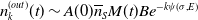 $ n_k^{(out)} (t) \sim A(0) \overline n_S M(t) B e^{ - k \psi (\sigma , E) }$
as
$ n_k^{(out)} (t) \sim A(0) \overline n_S M(t) B e^{ - k \psi (\sigma , E) }$
as
 $k \gg 1$
,
$k \gg 1$
,
 $N-k \gg 1$
, and
$N-k \gg 1$
, and
 $t \approx N$
.
$t \approx N$
.
Notice that both in the subcritical and in the supercritical case, we have that the asymptotic behaviour of
 $n_k^{(out)}$
as
$n_k^{(out)}$
as
 $k \to \infty$
is given by
$k \to \infty$
is given by
 $F(t) e^{- \lambda (\sigma , E) k }$
for a suitable function
$F(t) e^{- \lambda (\sigma , E) k }$
for a suitable function
 $F(t)$
encoding the change of mass in the system and a suitable exponent
$F(t)$
encoding the change of mass in the system and a suitable exponent
 $\lambda (\sigma , E )$
. The main difference between the supercritical and the subcritical case is that in the first case, when
$\lambda (\sigma , E )$
. The main difference between the supercritical and the subcritical case is that in the first case, when
 $\Delta \gt \Delta _c$
, we have that
$\Delta \gt \Delta _c$
, we have that
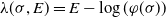 $\lambda (\sigma , E ) = E- \log (\varphi (\sigma ) )$
, hence
$\lambda (\sigma , E ) = E- \log (\varphi (\sigma ) )$
, hence
 $\lambda (\sigma , E)$
depends on the binding energy
$\lambda (\sigma , E)$
depends on the binding energy
 $\sigma$
. Instead, in the case
$\sigma$
. Instead, in the case
 $\Delta \lt \Delta _c$
, we have that
$\Delta \lt \Delta _c$
, we have that
 $\lambda (\sigma , E)$
does not depend on the binding energy
$\lambda (\sigma , E)$
does not depend on the binding energy
 $\sigma$
. Indeed, in that case, we have that
$\sigma$
. Indeed, in that case, we have that
 $\lambda (\sigma , E) = E$
. As we will see later in Subsection 4.3, the fact that
$\lambda (\sigma , E) = E$
. As we will see later in Subsection 4.3, the fact that
 $\lambda (\sigma , E)$
depends on
$\lambda (\sigma , E)$
depends on
 $\sigma$
when
$\sigma$
when
 $\Delta \gt \Delta _c$
is crucial in order to have strong discrimination properties.
$\Delta \gt \Delta _c$
is crucial in order to have strong discrimination properties.
4.1.3. Asymptotic behaviour in the critical case
$\Delta = \Delta _c$
when
$k \gg 1$
and
$N-k \gg 1$


By completeness, we also study the behaviour of
 $n_k$
as
$n_k$
as
 $k \to \infty$
in the critical case
$k \to \infty$
in the critical case
 $\Delta = \Delta _c$
. Under this assumption, we have that
$\Delta = \Delta _c$
. Under this assumption, we have that
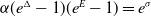 $\alpha (e^\Delta -1) (e^E-1) = e^\sigma$
. As in the case
$\alpha (e^\Delta -1) (e^E-1) = e^\sigma$
. As in the case
 $\Delta \neq \Delta _c$
, we have that the behaviour in the outer region is described by equation (4.3). We will now compute an explicit solution.
$\Delta \neq \Delta _c$
, we have that the behaviour in the outer region is described by equation (4.3). We will now compute an explicit solution.
Explicit solution to (4.3). First of all, we notice that when
 $\Delta = \Delta _c$
, we have that
$\Delta = \Delta _c$
, we have that
 \begin{equation*} \tilde {n}_k^{part} (t) = \frac { k e^{- k E } \tilde {n}_S(t)}{ \alpha (e^{\Delta + E} -1 )}, \quad k \in \mathbb N \end{equation*}
is a particular solution to (4.4). We now aim at finding a solution to the homogeneous equation corresponding to (4.4), i.e. to the following equation
 \begin{equation*} 0 =- \alpha \left (1+e^{E+ \Delta } \right ) \tilde {n}_k^{(out)} + \alpha e^E \tilde {n}_{k+1}^{(out)} + \alpha e^{\Delta } \tilde {n}_{k-1}^{(out)}, \quad k \in \mathbb N_0. \end{equation*}
In this case, we have homogeneous solutions of the form
 $n_k^{(hom)} =\theta (0)^k$
where
$n_k^{(hom)} =\theta (0)^k$
where
 $\theta (0)$
is a solution to
$\theta (0)$
is a solution to
 \begin{equation*} \theta (0)^2 - (e^\Delta + e^{- E} ) \theta (0) + e^{\Delta - E } =0. \end{equation*}
Notice that the two solutions
 $\theta _{1}(0)$
and
$\theta _{1}(0)$
and
 $\theta _2(0)$
to the second-order equation are given by
$\theta _2(0)$
to the second-order equation are given by
 \begin{equation*} \theta _2(0)=e^\Delta , \quad \theta _1(0)=e^{- E}. \end{equation*}
As before, the only admissible solution is
 $\theta _1(0)\lt 1$
. Therefore, the solution to equation (4.4) is
$\theta _1(0)\lt 1$
. Therefore, the solution to equation (4.4) is
 \begin{equation} \tilde {n}_k^{(out)}(t) =e^{-k E } \left ( \frac {k \tilde {n}_S(t) }{ \alpha (e^{\Delta + E} -1 )}+ F(t) \right ), \quad k \in \mathbb N \end{equation}
where
 $F(t)=\tilde {n}_0^{(out)}(t)$
and where
$F(t)=\tilde {n}_0^{(out)}(t)$
and where
 $\tilde {n}_0^{(out)} (t)$
can be computed by solving equation (4.3). Indeed, we have that
$\tilde {n}_0^{(out)} (t)$
can be computed by solving equation (4.3). Indeed, we have that
 \begin{equation*} 0=\tilde {n}_S (t) -(e^\sigma +\alpha e^\Delta ) \tilde {n}_0^{(out)} (t) + \alpha e^E \tilde {n}_1^{(out)} (t) = \tilde {n}_S (t) -(e^\sigma +\alpha e^\Delta ) \tilde {n}_0^{(out)} (t)+ \alpha \left ( \frac {\tilde {n}_S (t)}{ \alpha (e^{\Delta + E} -1 )}+ F(t) \right ) \end{equation*}
which implies that
 \begin{equation*} \tilde {n}_0^{(out)}(t)=\frac {e^\Delta }{ \alpha (e^{\Delta +E} -1 )(e^\Delta -1 )} \tilde {n}_S(t) . \end{equation*}
Asymptotic behaviour of
 $\boldsymbol{n_k^{(out)}}$
as
$\boldsymbol{n_k^{(out)}}$
as
 $\boldsymbol{k \to \infty}$
when
$\boldsymbol{k \to \infty}$
when
 $\boldsymbol{\Delta = \Delta _c}$
. Equality (4.12) implies that
$\boldsymbol{\Delta = \Delta _c}$
. Equality (4.12) implies that
 \begin{equation} \tilde {n}_k^{(out)} (t) \sim \frac { k e^{-k E } \tilde {n}_S(t) }{ \alpha (e^{\Delta + E} -1 )}\text{ as } k \to \infty . \end{equation}
The quasi steady state approximation implies that
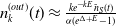 $ n_k^{(out)} (t) \approx \frac { k e^{-k E } \tilde {n}_S(t) }{ \alpha (e^{\Delta + E} -1 )}$
as
$ n_k^{(out)} (t) \approx \frac { k e^{-k E } \tilde {n}_S(t) }{ \alpha (e^{\Delta + E} -1 )}$
as
 $k \gg 1$
and
$k \gg 1$
and
 $N-k \gg 1$
and for
$N-k \gg 1$
and for
 $t \approx N$
. As in the subcritical case
$t \approx N$
. As in the subcritical case
 $\Delta \lt \Delta _c$
, in this case, we have that
$\Delta \lt \Delta _c$
, in this case, we have that
 $\lambda (\sigma , E) = E$
, hence
$\lambda (\sigma , E) = E$
, hence
 $\lambda (\sigma , E)$
does not depend on the binding energy
$\lambda (\sigma , E)$
does not depend on the binding energy
 $\sigma$
.
$\sigma$
.
4.2 Inner region:
$N-k \approx 1$
as
$N \to \infty$


We now study the behaviour of
 $n_k$
in the region in which
$n_k$
in the region in which
 $k = N-m$
and
$k = N-m$
and
 $m \approx 1$
. In this region,
$m \approx 1$
. In this region,
 $k$
is large and the dynamics is described by the equation for
$k$
is large and the dynamics is described by the equation for
 $n_k$
in (2.4), i.e.
$n_k$
in (2.4), i.e.
 \begin{align} \frac {d n_k }{dt} &= n_S e^{- k E} - ( e^{\sigma } + \alpha e^E + \alpha e^\Delta ) n_k + \alpha e^E n_{k+1} + \alpha e^{\Delta } n_{k-1} - \mu n_k, \quad k \in \{0, \ldots , N \} \nonumber\\ n_{ N+1}&=0. \end{align}
Notice that we are rewriting the equation for
 $n_N$
in (2.4), artificially introducing the state
$n_N$
in (2.4), artificially introducing the state
 $N+1$
in the model and imposing that
$N+1$
in the model and imposing that
 $n_{N+1}=0$
. This allows us to have the same equation to describe the evolution of
$n_{N+1}=0$
. This allows us to have the same equation to describe the evolution of
 $n_k$
for
$n_k$
for
 $k \lt N$
and for
$k \lt N$
and for
 $k =N$
.
$k =N$
.
Recall that
 $M$
changes in exponentially long times, i.e. for
$M$
changes in exponentially long times, i.e. for
 $t \approx e^{cN}$
for a positive constant
$t \approx e^{cN}$
for a positive constant
 $c$
. This allows us to approximate
$c$
. This allows us to approximate
 $n_k$
with a quasi steady state solution
$n_k$
with a quasi steady state solution
 $\tilde {n}_k$
. Since we assume that
$\tilde {n}_k$
. Since we assume that
 $ \mu \sim e^{- b N }$
as
$ \mu \sim e^{- b N }$
as
 $N \to \infty$
, this quasi steady state approximation for the solution to equation (4.14) satisfies the following system of equations
$N \to \infty$
, this quasi steady state approximation for the solution to equation (4.14) satisfies the following system of equations
 \begin{align} 0 &= \tilde {n}_S e^{- k E} - ( e^{\sigma } + \alpha e^E + \alpha e^\Delta ) \tilde {n}_k + \alpha e^{E } \tilde {n}_{k+1} + \alpha e^{\Delta } \tilde {n}_{k-1}, \quad k \in \{0, \ldots , N \} \nonumber\\ \tilde {n}_{N+1}&=0. \end{align}
Notice that the condition
 $ \tilde {n}_{N+1} =0$
plays the role of an absorbing boundary condition; indeed, when a complex reaches the state
$ \tilde {n}_{N+1} =0$
plays the role of an absorbing boundary condition; indeed, when a complex reaches the state
 $N+1$
, it is lost. This boundary condition, together with the n term
$N+1$
, it is lost. This boundary condition, together with the n term
 $\mu$
, is the reason why the total mass in our system slowly decreases in time when
$\mu$
, is the reason why the total mass in our system slowly decreases in time when
 $t \approx e^{cN }$
. In order to analyse the solution to (4.15), we consider the subcritical case from the supercritical case separately.
$t \approx e^{cN }$
. In order to analyse the solution to (4.15), we consider the subcritical case from the supercritical case separately.
4.2.1. Subcritical case
$\Delta \lt \Delta _c$

In order to study the solution to (4.15), it is convenient to consider the following change of variables
 \begin{equation} h_m (t) \,:\!=\, e^{(N-m)E} \tilde {n}_{N-m }(t) =e^{k E} \tilde {n}_k (t) \end{equation}
where we recall that
 $N-k=m$
. Therefore, we now study the following equation for
$N-k=m$
. Therefore, we now study the following equation for
 $h_m$
$h_m$
 \begin{align} 0 &= \tilde {n}_S(t) - ( e^{\sigma } + \alpha e^E + \alpha e^\Delta ) h_m (t)+ \alpha h_{m-1} (t) + \alpha e^{\Delta + E} h_{m+1} (t), \quad m \in \mathbb N \nonumber\\ h_{-1}(t)&=0, \nonumber\\ \lim _{m \to \infty } h_m(t) &= A(0) \tilde {n}_S(t) . \end{align}
We stress that the condition
 $h_{-1}(t)=0$
corresponds to
$h_{-1}(t)=0$
corresponds to
 $ \tilde {n}_{N+1}(t)=0$
. Instead, the condition on the limit of
$ \tilde {n}_{N+1}(t)=0$
. Instead, the condition on the limit of
 $h_m$
as
$h_m$
as
 $m \to \infty$
is a consequence of the matching with the behaviour of
$m \to \infty$
is a consequence of the matching with the behaviour of
 $ \tilde {n}_k$
in the outer region, i.e. (4.10).
$ \tilde {n}_k$
in the outer region, i.e. (4.10).
Notice that
 $h^{(p)}_m = A(0) n_S(t)$
is a particular solution to equation (4.17). We now study the homogeneous solutions to equation (4.17), i.e. solutions to (4.17) without the source term. In particular, we look for homogeneous solutions of the form
$h^{(p)}_m = A(0) n_S(t)$
is a particular solution to equation (4.17). We now study the homogeneous solutions to equation (4.17), i.e. solutions to (4.17) without the source term. In particular, we look for homogeneous solutions of the form
 \begin{equation*} h^{(h)}_m =\Theta ^m, \quad \forall m \in \mathbb N. \end{equation*}
Substituting this ansatz in equation (4.17), we obtain that
 $\Theta$
must satisfy the following equation
$\Theta$
must satisfy the following equation
 \begin{equation*} \Theta ^2 - \frac { \Omega (0)}{\alpha e^{E+\Delta }} \Theta + e^{-(E+ \Delta ) } =0 . \end{equation*}
This equation has two solutions
 $\Theta _{1}$
and
$\Theta _{1}$
and
 $\Theta _2$
given by
$\Theta _2$
given by
 \begin{equation*} \Theta _{1} = \frac {1}{2 \alpha e^{E+\Delta } } \left ( \Omega (0) - \sqrt {\Omega (0)^2 - 4 \alpha ^2 e^{E+\Delta }} \right ) \text{ and } \Theta _{2} = \frac {1}{2 \alpha e^{E+\Delta } } \left ( \Omega (0) + \sqrt {\Omega (0)^2 - 4 \alpha ^2 e^{E+\Delta }} \right )\! . \end{equation*}
Notice that since we expect the limit as
 $m \to \infty$
of
$m \to \infty$
of
 $ h_m$
to be finite for every fixed time
$ h_m$
to be finite for every fixed time
 $t\gt 0$
, then
$t\gt 0$
, then
 $\Theta ^m$
is an admissible homogeneous solution only when
$\Theta ^m$
is an admissible homogeneous solution only when
 $\Theta \leq 1$
. Moreover, since
$\Theta \leq 1$
. Moreover, since
 $\Delta \lt \Delta _c$
, then we have that
$\Delta \lt \Delta _c$
, then we have that
 \begin{equation*} \Theta _2 = \frac {1}{2 \alpha e^{E+\Delta } } \left ( \Omega (0) + \sqrt {\Omega (0)^2 - 4 \alpha ^2 e^{E+\Delta }} \right ) \gt 1. \end{equation*}
Hence, there exists a unique admissible homogeneous solution, which is
 \begin{equation*} \Theta _1= \frac {1}{2 \alpha e^{E+\Delta } } \left ( \Omega (0) - \sqrt {\Omega (0)^2 - 4 \alpha ^2 e^{E+\Delta }} \right ) = \varphi (\sigma ) e^{- (E+\Delta ) } \lt 1. \end{equation*}
As a consequence, the solution to (4.17) is given by
 \begin{align*} h_m(t) = h_m^{(p)} (t)+ h_m^{(h)} (t)= A(0) \tilde {n}_S (t)+ F(t) \Theta ^m = A(0) \tilde {n}_S(t) + F(t) \varphi (\sigma )^m e^{- m (E+ \Delta ) }, \quad m \in \mathbb N \cup \{ -1\}. \end{align*}
Moreover, the condition
 $h_{-1}=0$
implies that
$h_{-1}=0$
implies that
 \begin{equation*} F(t) = - A(0) \varphi (\sigma ) e^{- (E+\Delta ) } \tilde {n}_S(t) . \end{equation*}
Summarizing, we have that
 \begin{equation*} h_m = A(0) \tilde {n}_S ( 1 - \varphi (\sigma )^{m+1} e^{- (m+1) (E+ \Delta ) })\quad m \in \mathbb N \cup \{ -1\}. \end{equation*}
Hence, we obtain that
 \begin{equation} \tilde {n}_{N} (t) \sim e^{- N E } h_0= e^{- N E } A(0) ( 1 - \varphi (\sigma ) e^{- (E+ \Delta ) }) \tilde {n}_S(t) \text{ as } N \to \infty . \end{equation}
Using the quasi steady state approximation
 $\tilde {n}_{N} (t) \approx n_{N} (t)$
for
$\tilde {n}_{N} (t) \approx n_{N} (t)$
for
 $t \approx N$
we deduce that
$t \approx N$
we deduce that
 \begin{equation*} n_{N} (t) \sim e^{- N E } h_0= e^{- N E } A(0) ( 1 - \varphi (\sigma ) e^{- (E+ \Delta ) }) \tilde {n}_S(t) \text{ as } N \to \infty , \ t \approx N. \end{equation*}
Here, we stress again that the asymptotic behaviour of
 $n_N$
as
$n_N$
as
 $N \to \infty$
is of the form
$N \to \infty$
is of the form
 $ F(t) e^{- N \lambda (\sigma , E) }$
where the parameter
$ F(t) e^{- N \lambda (\sigma , E) }$
where the parameter
 $\lambda (\sigma , E)$
, in this subcritical case
$\lambda (\sigma , E)$
, in this subcritical case
 $\Delta \lt \Delta _c$
, does not depend on
$\Delta \lt \Delta _c$
, does not depend on
 $\sigma$
and where
$\sigma$
and where
 $F(t)$
is a suitable function of time.
$F(t)$
is a suitable function of time.
4.2.2. Supercritical case
$\Delta \gt \Delta _c$

As we did in the subcritical case (see (4.16)), we remove the leading exponential behaviour by using the change of variables
 \begin{equation*} \ell _k = e^{ k \lambda (\sigma ) } \tilde {n}_k = e^{ k E - k \log (\varphi (\sigma )) } \tilde {n}_k, \end{equation*}
where
 $\lambda$
is defined as (2.10). Performing the change of variable in equation (4.15), we deduce that
$\lambda$
is defined as (2.10). Performing the change of variable in equation (4.15), we deduce that
 $\ell _k$
must satisfy the following equation
$\ell _k$
must satisfy the following equation
 \begin{align*} 0 &= \tilde {n}_S(t) - ( e^{\sigma } + \alpha e^E + \alpha e^\Delta) e^{ k \log (\varphi (\sigma )) } \ell _k(t) + \alpha e^{ (k +1)\log (\varphi (\sigma )) } \ell _{k+1} (t) + \alpha e^{\Delta + E + ( k-1) \log (\varphi (\sigma )) } \ell _{k-1}(t) \\ 0& =\ell _{N+1}(t) \end{align*}
Since we are analysing the behaviour in the inner region where
 $k \gg 1$
, we have that
$k \gg 1$
, we have that
 $\tilde {n}_S \ll e^{ k \log (\varphi (\sigma )) } \ell _k$
,
$\tilde {n}_S \ll e^{ k \log (\varphi (\sigma )) } \ell _k$
,
 $\tilde {n}_S \ll e^{\Delta + E + ( k-1) \log (\varphi (\sigma )) } \ell _{k-1}$
, and
$\tilde {n}_S \ll e^{\Delta + E + ( k-1) \log (\varphi (\sigma )) } \ell _{k-1}$
, and
 $\tilde {n}_S \ll e^{ (k +1)\log (\varphi (\sigma )) } \ell _{k+1}$
. Therefore, we can approximate the equation above as follows
$\tilde {n}_S \ll e^{ (k +1)\log (\varphi (\sigma )) } \ell _{k+1}$
. Therefore, we can approximate the equation above as follows
 \begin{align*} 0 & \sim - ( e^{\sigma } + \alpha e^E + \alpha e^\Delta ) \varphi (\sigma ) \ell _k (t)+ \alpha \varphi (\sigma )^2 \ell _{k+1}(t) + \alpha e^{\Delta + E } \ell _{k-1} (t), \text{ as } k \to \infty \\ 0&= \ell _ {N+1}(t) \end{align*}
Moreover, we define
 $h_m = \ell _{N-m }$
. Then
$h_m = \ell _{N-m }$
. Then
 $h_m$
satisfies the following equation
$h_m$
satisfies the following equation
 \begin{align*} 0 & = - ( e^{\sigma } + \alpha e^E + \alpha e^\Delta ) \varphi (\sigma ) h_m(t) + \alpha \varphi (\sigma )^2 h_{m-1} (t) + \alpha e^{\Delta + E } h_{m+1} (t), \quad m \in \mathbb N \\ h_{-1}(t)&=0 \\ \lim _{m \to \infty } h_m (t)&=B A (0) \tilde {n}_S(t) \end{align*}
where the last equality comes from the matching condition; indeed, for
 $k \gg 1$
and
$k \gg 1$
and
 $N-k \gg 1$
, we have that the behaviour of
$N-k \gg 1$
, we have that the behaviour of
 $\tilde {n}_k$
is given by (4.11).
$\tilde {n}_k$
is given by (4.11).
We make the ansatz
 $h_m(t) = \Theta ^m$
for every
$h_m(t) = \Theta ^m$
for every
 $m \in \mathbb N$
and obtain that
$m \in \mathbb N$
and obtain that
 \begin{equation*} \alpha e^{\Delta + E } \Theta ^2 - \Omega (0) \varphi (\sigma ) \Theta + \alpha (\varphi (\sigma ))^2 =0. \end{equation*}
We deduce that
 \begin{equation*} \Theta _{12} = \frac {\varphi (\sigma )}{2\alpha e^{\Delta + E }} \left ( \Omega (0) \pm \sqrt {\Omega (0)^2 - 4 \alpha ^2 e^{E+\Delta }} \right ) \end{equation*}
In particular, we obtain that
 \begin{equation*} \Theta _1 = \frac {\varphi (\sigma )}{2\alpha e^{\Delta + E }} \left ( \Omega (0) - \sqrt {\Omega (0)^2 - 4 \alpha ^2 e^{E+\Delta }} \right ) = \varphi (\sigma )^2 e^{- (\Delta + E ) } \end{equation*}
and
 \begin{equation*} \Theta _2 = \frac {\varphi (\sigma )}{2\alpha e^{\Delta + E }} \left ( \Omega (0) + \sqrt {\Omega (0)^2 - 4 \alpha ^2 e^{E+\Delta }} \right ) = 1 \end{equation*}
Both these solutions are admissible as they are both smaller than or equal to one. We deduce that
 \begin{equation*} h_m(t) = F_1(t) + F_2(t) e^{ 2m \log \varphi (\sigma ) - m (\Delta + E ) }, \quad \forall m \in \mathbb N \cup \{ -1 \}. \end{equation*}
Matching the behaviour in the inner with the behaviour in the outer region implies that
 $F_1 (t)= B A(0) n_S(t)$
. On the other hand, since
$F_1 (t)= B A(0) n_S(t)$
. On the other hand, since
 $h_{-1} (t)=0$
, we also have that
$h_{-1} (t)=0$
, we also have that
 \begin{equation*} F_2(t) = - F_1 (t) e^{ -(\Delta + E)} (\varphi (\sigma ))^2= - B A(0) n_S(t)e^{- ( \Delta + E )}(\varphi (\sigma ))^2, \end{equation*}
where we recall that
 $B$
is given by (4.9). Summarizing, we have that
$B$
is given by (4.9). Summarizing, we have that
 \begin{equation*} h_m(t) = B A(0) \left ( 1 - e^{ 2(m+1) \log \varphi (\sigma ) - (m+1) (\Delta + E ) } \right ) \tilde {n}_S (t), \quad \forall m \in \mathbb N \cup \{ -1 \} \end{equation*}
therefore, we have that when
 $t \approx N$
it holds that
$t \approx N$
it holds that
 \begin{equation} n_{N}(t) \sim e^{- NE + N \log (\varphi (\sigma )) } h_0 (t)= e^{- N E + N \log (\varphi (\sigma )) } A(0) B ( 1 - ( \varphi (\sigma ))^2 e^{ - (\Delta + E ) } ) \tilde {n}_S (t), \text{ as } N \to \infty . \end{equation}
Notice that the asymptotic behaviour of
 $n_N$
as
$n_N$
as
 $N \to \infty$
is of the form
$N \to \infty$
is of the form
 $ F(t) e^{- N \lambda (\sigma , E)}$
where
$ F(t) e^{- N \lambda (\sigma , E)}$
where
 $\lambda (\sigma ,E)$
depends on
$\lambda (\sigma ,E)$
depends on
 $\sigma$
where
$\sigma$
where
 $F(t)$
is a function of time that takes into account the change of mass, notice that this function changes very slowly in time, more precisely in time scales much larger than
$F(t)$
is a function of time that takes into account the change of mass, notice that this function changes very slowly in time, more precisely in time scales much larger than
 $N$
.
$N$
.
4.2.3. Critical case
$\Delta = \Delta _c$

For completeness, we now analyse the behaviour of
 $\tilde {n}_k$
in the inner region under the assumption that
$\tilde {n}_k$
in the inner region under the assumption that
 $\Delta = \Delta _c$
. To this end, we make the change of variables
$\Delta = \Delta _c$
. To this end, we make the change of variables
 $\ell _k \,:\!=\, \frac { e^{k E}}{k} \tilde {n}_k$
in equation (4.15) and deduce that
$\ell _k \,:\!=\, \frac { e^{k E}}{k} \tilde {n}_k$
in equation (4.15) and deduce that
 $\ell _k$
satisfies
$\ell _k$
satisfies
 \begin{align} 0 &= \tilde {n}_S (t) - ( e^{\sigma } + \alpha e^E + \alpha e^\Delta ) k \ell _k (t) + \alpha (k+1) \ell _{k+1} (t) + \alpha e^{\Delta +E} (k-1) \ell _{k-1} (t), \quad k \in \{ 0, \ldots , N \} \nonumber\\ 0 &=\ell _{N+1} (t). \end{align}
Since in the inner region we have that
 $k \gg 1$
, then
$k \gg 1$
, then
 $\tilde {n}_S$
is of lower order with respect to the other terms in the equation. Therefore, we approximate equation (4.20) with the following homogeneous equation
$\tilde {n}_S$
is of lower order with respect to the other terms in the equation. Therefore, we approximate equation (4.20) with the following homogeneous equation
 \begin{align} 0 &= - ( e^{\sigma } + \alpha e^E + \alpha e^\Delta ) k \ell _k (t) + \alpha (k+1) \ell _{k+1} (t) + \alpha e^{\Delta +E} (k-1) \ell _{k-1} (t) \text{ as } k \to \infty \nonumber\\ \ell _{N+1}(t) &=0. \end{align}
In order to match the behaviour in the inner region with the behaviour in the outer region, it is convenient to consider the change of variable
 $k = N-m$
and to study
$k = N-m$
and to study
 $h_{m} \,:\!=\, (N-m) \ell _{N-m}$
. Notice that, due to its definition,
$h_{m} \,:\!=\, (N-m) \ell _{N-m}$
. Notice that, due to its definition,
 $h_{m}$
satisfies the following equation
$h_{m}$
satisfies the following equation
 \begin{align} 0 &= - ( e^{\sigma } + \alpha e^E + \alpha e^\Delta ) h_m(t) + \alpha h_{m-1} (t) + \alpha e^{\Delta +E} h_{m+1} (t)\nonumber \\ h_{-1}(t)&=0, \quad m \in \mathbb N \nonumber \\ \lim _{m \to \infty } h_m (t) &= \frac { \tilde {n}_S(t) }{\alpha (e^{\Delta + E } -1 ) } . \end{align}
Notice that the last condition comes from the matching with the outer region, i.e. by the fact that the behaviour in the outer region is given by (4.13).
Since the equation for
 $h_m$
is homogeneous, it has solutions of the form
$h_m$
is homogeneous, it has solutions of the form
 $h_m= \theta ^m$
where
$h_m= \theta ^m$
where
 $\theta$
satisfies
$\theta$
satisfies
 \begin{equation*} \theta ^2 - \left ( \frac { 1+ e^{\Delta + E } }{e^{\Delta + E }}\right ) + \frac {1}{e^{\Delta + E }}=0 . \end{equation*}
We deduce that both
 $\theta _1^m = 1$
and
$\theta _1^m = 1$
and
 $\theta _2^m = e^{-m (\Delta + E) }$
are admissible solutions to (4.22). Therefore, we have that the sequence
$\theta _2^m = e^{-m (\Delta + E) }$
are admissible solutions to (4.22). Therefore, we have that the sequence
 $\{ h_m\}_{m}$
given by
$\{ h_m\}_{m}$
given by
 \begin{equation*} h_m(t) = F_1(t) + F_2(t) e^{-m (\Delta + E) }, \end{equation*}
with
 $F_2=-F_1e^{- (\Delta + E) }$
and with
$F_2=-F_1e^{- (\Delta + E) }$
and with
 \begin{equation*} F_1(t) = \frac {\tilde {n}_S (t)}{\alpha (e^{\Delta + E} - 1 ) }, \end{equation*}
is the solution to (4.22). In particular, we conclude that
 $h_0 = \frac {n_S (t) } {\alpha e^{\Delta + E} }$
, and therefore,
$h_0 = \frac {n_S (t) } {\alpha e^{\Delta + E} }$
, and therefore,
 \begin{equation} n_{N} (t) \sim \frac {\tilde {n}_S(t)}{\alpha e^{E+\Delta } } N e^{-N E } \text{ as } N \to \infty \text{ and } t \approx N. \end{equation}
4.3. Discrimination property
We now study the discrimination property of the model under different assumptions on
 $\Delta$
. To this end, we analyse the probability of response
$\Delta$
. To this end, we analyse the probability of response
 $p_{res}$
defined as in (2.7) as
$p_{res}$
defined as in (2.7) as
 $N \to \infty$
in the different regimes, subcritical, critical and supercritical using the asymptotics (4.18), (4.19), (4.23) for
$N \to \infty$
in the different regimes, subcritical, critical and supercritical using the asymptotics (4.18), (4.19), (4.23) for
 $n_N$
.
$n_N$
.
Subcritical case
 $\boldsymbol{\Delta \lt \Delta _c}$
. Using the asymptotics for
$\boldsymbol{\Delta \lt \Delta _c}$
. Using the asymptotics for
 $n_{N}$
in (4.18), we approximate the probability of response as follows
$n_{N}$
in (4.18), we approximate the probability of response as follows
 \begin{align*} p_{res} (\sigma ) = \alpha e^\Delta \int _0^\infty n_{N} (t) dt \approx \alpha e^{\Delta } e^{-NE} A(0) \overline n_S \left (1- \varphi (\sigma ) e^{-(E+ \Delta )} \right ) \int _0^\infty M (t) dt \text{ as } N \to \infty . \end{align*}
In the approximation above, we are using that the region where
 $t \approx N$
gives the main contribution to the integral
$t \approx N$
gives the main contribution to the integral
 $\int _0^\infty n_N(t) dt$
. Moreover, notice that we have that
$\int _0^\infty n_N(t) dt$
. Moreover, notice that we have that
 \begin{equation} \frac {dM }{dt} = - \mu M - \alpha e^{\Delta } n_{N} \sim - ( \mu + \alpha e^{\Delta } e^{-NE} A(0) \overline n_S (1- \varphi (\sigma ) e^{-(E+ \Delta )} ) ) M (t) \text{ as } N \to \infty . \end{equation}
Notice that equation (4.24) implies that the mass changes in exponentially large time scales. More precisely, we have that
 \begin{equation} M(t) \sim e^{- \left ( \mu + \alpha e^{\Delta } e^{-NE} A(0) \overline n_S \left (1- \varphi (\sigma ) e^{-(E+ \Delta )} \right ) \right ) t } \text{ as } N \to \infty . \end{equation}
Using this approximation for
 $M$
, we deduce that
$M$
, we deduce that
 \begin{equation} p_{res} (\sigma ) \approx \left ( 1 +\frac {\mu e^{NE}}{ \alpha e^{\Delta } A(0) \overline n_S \left (1- \varphi (\sigma ) e^{-(E+ \Delta )} \right ) } \right )^{-1} \text{ as } N \to \infty . \end{equation}
Using the fact that
 $\mu \sim e^{- b N }$
as
$\mu \sim e^{- b N }$
as
 $N \to \infty$
, we obtain that
$N \to \infty$
, we obtain that
 \begin{equation*} p_{res}(\sigma ) \approx ( 1 + C_1e^{N(E- b)} )^{-1} \text{ as } N \to \infty . \end{equation*}
where
 $C_1\,:\!=\,\left [ \alpha e^{\Delta } A(0) \overline n_S \left (1- \varphi (\sigma ) e^{-E- \Delta } \right ) \right ]^{-1}$
. In particular, we conclude that
$C_1\,:\!=\,\left [ \alpha e^{\Delta } A(0) \overline n_S \left (1- \varphi (\sigma ) e^{-E- \Delta } \right ) \right ]^{-1}$
. In particular, we conclude that
 $p_N \approx 0$
when
$p_N \approx 0$
when
 $E\gt b$
,
$E\gt b$
,
 $p_N \approx 1$
as
$p_N \approx 1$
as
 $N \to \infty$
if
$N \to \infty$
if
 $E\lt b$
. Notice that in this case, if we plot the probability
$E\lt b$
. Notice that in this case, if we plot the probability
 $p_{res} (\sigma )$
, defined as (2.7), as a function of
$p_{res} (\sigma )$
, defined as (2.7), as a function of
 $\sigma$
, we do not have a sharp transition from
$\sigma$
, we do not have a sharp transition from
 $0$
to
$0$
to
 $1$
around a critical binding energy
$1$
around a critical binding energy
 $\sigma _c$
(see Figure 2). The dependence on
$\sigma _c$
(see Figure 2). The dependence on
 $\sigma$
is encoded only in the constant
$\sigma$
is encoded only in the constant
 $C_1$
.
$C_1$
.
Critical case
 $\boldsymbol{\Delta = \Delta _c}$
. Arguing as in the subcritical case
$\boldsymbol{\Delta = \Delta _c}$
. Arguing as in the subcritical case
 $\Delta \lt \Delta _c$
, we deduce that (4.23) implies
$\Delta \lt \Delta _c$
, we deduce that (4.23) implies
 \begin{equation*} p_{res} (\sigma ) \approx \left ( 1 + \frac {e^{N(E-b)}}{ N \overline n_S } \right )^{-1} \text{ as } N \to \infty \end{equation*}
We conclude that
 $p_{res} (\sigma ) \approx 0$
as
$p_{res} (\sigma ) \approx 0$
as
 $N \to \infty$
when
$N \to \infty$
when
 $E\gt b$
, while
$E\gt b$
, while
 $p_{res} (\sigma ) \approx 1$
as
$p_{res} (\sigma ) \approx 1$
as
 $N \to \infty$
if
$N \to \infty$
if
 $E \leq b$
. The situation is similar to the one that we have for the subcritical case
$E \leq b$
. The situation is similar to the one that we have for the subcritical case
 $\Delta \lt \Delta _c$
.
$\Delta \lt \Delta _c$
.
Supercritical case
 $\boldsymbol{\Delta \gt \Delta _c}$
. Using the approximation for
$\boldsymbol{\Delta \gt \Delta _c}$
. Using the approximation for
 $n_{N}$
as
$n_{N}$
as
 $N \to \infty$
given in (4.19), we deduce that
$N \to \infty$
given in (4.19), we deduce that
 \begin{equation} p_{res} (\sigma ) \approx \left ( 1+C_2 e^{(E -b- \log (\varphi (\sigma ) ) N }\right )^{-1} \end{equation}
where
 $C_2= \left [ \alpha e^\Delta B A(0) \overline n_S \left ( 1- (\varphi (\sigma ))^2 e^{ - (\Delta + E) } \right ) \right ]^{-1}$
. Recall that
$C_2= \left [ \alpha e^\Delta B A(0) \overline n_S \left ( 1- (\varphi (\sigma ))^2 e^{ - (\Delta + E) } \right ) \right ]^{-1}$
. Recall that
 $\varphi (\sigma )$
is a function of
$\varphi (\sigma )$
is a function of
 $\sigma$
, indeed
$\sigma$
, indeed
 \begin{equation*} \varphi (\sigma )= \frac {1}{2 \alpha } \left ( e^\sigma + \alpha (e^\Delta + e^E) - \sqrt {(e^\sigma + \alpha (e^\Delta + e^E) )^2 - 4 \alpha ^2 e^{\Delta + E} } \right ). \end{equation*}
Moreover, notice that
 \begin{equation*} \varphi '(\sigma )= \frac {e^\sigma }{2 \alpha } \left ( 1 - \frac {e^\sigma + \alpha (e^\Delta + e^E) }{ \sqrt {(e^\sigma + \alpha (e^\Delta + e^E) )^2 - 4 \alpha ^2 e^{\Delta + E} } } \right ) \lt 0, \end{equation*}
hence the function
 $\varphi$
is strictly decreasing. In particular, this implies that the function
$\varphi$
is strictly decreasing. In particular, this implies that the function
 $\lambda (\sigma , E)=$
 $E- \log (\varphi (\sigma ))$
is increasing in
$E- \log (\varphi (\sigma ))$
is increasing in
 $\sigma$
. As a consequence, if we assume that
$\sigma$
. As a consequence, if we assume that
 \begin{equation} \lim _{\sigma \to \infty } \lambda (\sigma , E) = E\gt b \gt \max \{ E - \Delta , 0 \} = \lim _{\sigma \to - \infty } \lambda (\sigma , E), \end{equation}
then we have that there exists
 $\sigma _c \in \mathbb R$
such that
$\sigma _c \in \mathbb R$
such that
 $\lambda (\sigma _c , E) = b$
. Notice that if we consider
$\lambda (\sigma _c , E) = b$
. Notice that if we consider
 $p_{res}$
as a function of
$p_{res}$
as a function of
 $\sigma$
, we see a sharp transition from
$\sigma$
, we see a sharp transition from
 $1$
to
$1$
to
 $0$
, i.e. from response to non-response, around the critical binding energy
$0$
, i.e. from response to non-response, around the critical binding energy
 $\sigma _c$
. The region in which the transition takes place is the region in which we have that
$\sigma _c$
. The region in which the transition takes place is the region in which we have that
 \begin{equation*} |\lambda (\sigma , E) - \lambda (\sigma _c, E) | \lesssim \frac {1}{N }. \end{equation*}
This region tends to
 $0$
as
$0$
as
 $N \to \infty$
. If instead we have that
$N \to \infty$
. If instead we have that
 $\sigma$
is such that
$\sigma$
is such that
 $\lambda (\sigma , E ) - \lambda (\sigma _c, E ) \gt \frac {1}{N }$
then we have
$\lambda (\sigma , E ) - \lambda (\sigma _c, E ) \gt \frac {1}{N }$
then we have
 $p_{res}(\sigma ) \approx 1$
as
$p_{res}(\sigma ) \approx 1$
as
 $N \to \infty$
and if
$N \to \infty$
and if
 $\lambda (\sigma _c, E) - \lambda (\sigma , E) \gt \frac {1}{N }$
then we have
$\lambda (\sigma _c, E) - \lambda (\sigma , E) \gt \frac {1}{N }$
then we have
 $p_{res} (\sigma ) \approx 0$
as
$p_{res} (\sigma ) \approx 0$
as
 $N \to \infty$
.
$N \to \infty$
.
Notice that the discrimination property that we obtain for
 $\Delta \gt \Delta _c$
relies on the fact that we assume that the interaction between the ligands and the receptors takes place in a characteristic time, the signalling lifetime
$\Delta \gt \Delta _c$
relies on the fact that we assume that the interaction between the ligands and the receptors takes place in a characteristic time, the signalling lifetime
 $\mu ^{-1 }$
. If we assume that the ligand can interact with the receptor for an arbitrarily long amount of time, the discrimination property is lost.
$\mu ^{-1 }$
. If we assume that the ligand can interact with the receptor for an arbitrarily long amount of time, the discrimination property is lost.
5. Approximated model on
$\mathbb N$

In this section, we study in detail the model that we obtain taking the limit as
 $N \to \infty$
in (2.4). Analysing this model rigorously using Laplace transform methods is easier than analysing the model with a finite number of states
$N \to \infty$
in (2.4). Analysing this model rigorously using Laplace transform methods is easier than analysing the model with a finite number of states
 $N$
. Moreover, the behaviour of the model on the half line gives insights on the behaviour of the model with a finite number of states
$N$
. Moreover, the behaviour of the model on the half line gives insights on the behaviour of the model with a finite number of states
 $N$
when
$N$
when
 $N$
is large. Indeed, we prove that if
$N$
is large. Indeed, we prove that if
 $\Delta \lt \Delta _c$
, then the solution to the problem on the half line is such that as
$\Delta \lt \Delta _c$
, then the solution to the problem on the half line is such that as
 $t \to \infty$
 \begin{equation*} n_k(t) \sim A(0) \overline n_S e^{- k E} \text{ for } k \approx t, \ t \to \infty \end{equation*}
We refer to Theorem5.8 for the rigorous statement. If instead
 $\Delta \gt \Delta _c$
, then
$\Delta \gt \Delta _c$
, then
 \begin{equation*} n_k(t) \sim B(0) A(0) \overline n_S e^{- k (E- \log (\varphi (\sigma ))} \text{ for } k \lesssim t , \ t \to \infty \end{equation*}
while
 \begin{equation*} e^{ k (E- \log (\varphi (\sigma ))} n_k (t) \ll 1 \text{ for } k \gtrsim t, \ t \to \infty . \end{equation*}
We refer to Theorem5.9 for the rigorous statement. Notice that the results that we obtain for this model are consistent with the formal arguments in Section 4. Moreover, notice that when
 $k \approx t$
, we have that
$k \approx t$
, we have that
 $n_k(t)$
is at steady state. This is consistent with the assumption that
$n_k(t)$
is at steady state. This is consistent with the assumption that
 $n_N(t)$
stabilizes in time scales of order
$n_N(t)$
stabilizes in time scales of order
 $N$
that we make in Section 4.
$N$
that we make in Section 4.
The system of ODEs that we study in this section is the one that we obtain taking the limit as
 $N \to \infty$
in (2.4), i.e.
$N \to \infty$
in (2.4), i.e.
 \begin{align} \frac {d n_S }{dt} &= - n_S - \frac {e^{- E} }{ 1- e^{- E}} n_S + e^{\sigma } \sum _{k=0}^{\infty } n_k \nonumber \\ \frac {d n_0 }{dt} &= n_S - e^{\sigma } n_0 + \alpha e^E n_1 - \alpha e^{\Delta } n_0 \nonumber \\[4pt] \frac {d n_k }{dt} &= n_S e^{- k E} - ( e^{\sigma } + \alpha e^E + \alpha e^\Delta ) n_k + \alpha e^E n_{k+1} + \alpha e^{\Delta } n_{k-1} \end{align}
with initial datum
 $n(0)=(1, 0, \ldots , 0)$
. Notice that since
$n(0)=(1, 0, \ldots , 0)$
. Notice that since
 $(n_S, n_0, \ldots , n_N)$
is the vector of the probabilities of reaching the different states of the system in the time interval
$(n_S, n_0, \ldots , n_N)$
is the vector of the probabilities of reaching the different states of the system in the time interval
 $(0, t]$
, we have that
$(0, t]$
, we have that
 $M(t) = n_S (t) + \sum _{k=0}^{\infty } n_k(t) =1.$
Taking Laplace transforms in all the terms in (5.1), we obtain the following systems of equations for the vector of Laplace transforms
 $(\hat {n}_S (z), \hat {n}_0(z), \hat {n}_1(z), \ldots , \hat {n}_{N-1}(z) )$
of
$(\hat {n}_S (z), \hat {n}_0(z), \hat {n}_1(z), \ldots , \hat {n}_{N-1}(z) )$
of
 $(n_S(t), n_0(t), n_1(t), \ldots ,n_{N-1} (t))$
 \begin{align} \left ( z + \frac {1}{1-e^{- E}} \right ) \hat { n}_S &= 1+ e^{\sigma } \sum _{k=0}^{\infty } \hat {n}_k \nonumber\\[3pt] \left ( e^{\sigma } +z + \alpha e^{\Delta } \right ) \hat {n}_0 &= \hat { n}_S + \alpha e^E \hat { n}_1 \nonumber\\[3pt] \Omega (z) \hat {n}_k &= \hat {n}_S e^{- k E} + \alpha e^E \hat {n}_{k+1} + \alpha e^{\Delta } \hat {n}_{k-1} \quad k \in \mathbb N_0 , \end{align}
where
 $ z \in \mathbb C$
and where we use the notation
$ z \in \mathbb C$
and where we use the notation
 \begin{equation} \Omega (z)\,:\!=\, z+ e^{\sigma } + \alpha e^{\Delta } + \alpha e^{E}. \end{equation}
We will compute now explicit solutions to (5.2). As a first step, we compute
 $\hat {n}_S$
.
$\hat {n}_S$
.
Lemma 5.1.
Assume that the vector
 $(\hat {n}_S (z), \hat {n}_0(z), \hat {n}_1(z), \ldots , \hat {n}_{N-1}(z) )$
is a solution to (5.2). Then, the function
$(\hat {n}_S (z), \hat {n}_0(z), \hat {n}_1(z), \ldots , \hat {n}_{N-1}(z) )$
is a solution to (5.2). Then, the function
 $\hat {n}_S$
is analytic for every
$\hat {n}_S$
is analytic for every
 $z \in \mathbb C \setminus \{ z_S, 0 \}$
where
$z \in \mathbb C \setminus \{ z_S, 0 \}$
where
 \begin{equation} z_S \,:\!=\, - \left ( \frac {1}{1-e^{- E}} + e^\sigma \right ). \end{equation}
More precisely, we have that
 \begin{equation} \hat { n}_S(z) = \frac {z+ e^\sigma }{ z \left ( z - z_S\right ) }. \end{equation}
Proof. Since in this model we have that
 $\frac {d M(t)}{dt} =0$
, we deduce that
$\frac {d M(t)}{dt} =0$
, we deduce that
 \begin{equation*} z \left ( \hat {n}_S + \sum _{k=0}^{\infty } \hat {n}_k \right ) =1. \end{equation*}
Hence, the equation for
 $\hat {n}_S$
can be rewritten as
$\hat {n}_S$
can be rewritten as
 \begin{equation*} \left ( z + \frac {1}{1-e^{- E}} \right ) \hat { n}_S = e^{\sigma } \left ( \frac {1}{z} - \hat { n}_S \right ) +1 \end{equation*}
This implies that (5.5) holds.
We find now a particular solution to (5.2). To this end, it is convenient to define the function
 $A\,:\, \mathbb C \rightarrow \mathbb C$
, which is given by
$A\,:\, \mathbb C \rightarrow \mathbb C$
, which is given by
 \begin{equation} A (z) \,:\!=\, \frac {1}{z-z_A}=\frac {1}{\Omega (z) - \alpha \left ( 1+e^{E+ \Delta } \right ) } \quad z \in \mathbb C, \end{equation}
where
 \begin{equation} z_A \,:\!=\, \alpha (e^{E} -1 ) (e^{\Delta } -1 )- e^\sigma . \end{equation}
Lemma 5.2.
Assume that the function
 $\hat {n}_0\,:\, \mathbb C \rightarrow \mathbb C$
is given and let
$\hat {n}_0\,:\, \mathbb C \rightarrow \mathbb C$
is given and let
 $\hat {n}_S$
be given by (5.5). We define the sequence
$\hat {n}_S$
be given by (5.5). We define the sequence
 $\{ \hat {n}_k^{(p)}\}_{k=1}^\infty$
of functions
$\{ \hat {n}_k^{(p)}\}_{k=1}^\infty$
of functions
 $\hat {n}_k^{(p)}\,:\, \mathbb C \rightarrow \mathbb C$
given by
$\hat {n}_k^{(p)}\,:\, \mathbb C \rightarrow \mathbb C$
given by
 \begin{equation} \hat {n}_k^{(p)} (z)= A(z)e^{- k E} \hat {n}_S(z),\quad k \in \mathbb N_0. \end{equation}
The sequence
 $\{ \hat {n}_k^{(p)}\}_{k=1}^\infty$
is a particular solution to
$\{ \hat {n}_k^{(p)}\}_{k=1}^\infty$
is a particular solution to
 \begin{align} \Omega (z) \hat {n}_k &= \hat {n}_S e^{- k E} + \alpha e^E \hat {n}_{k+1} + \alpha e^{\Delta } \hat {n}_{k-1} \quad k \in \mathbb N_0, \end{align}
Proof. We substitute (5.8) in the equation for
 $\hat {n}_k$
and obtain that
$\hat {n}_k$
and obtain that
 \begin{equation*} \Omega (z) \hat {n}_k(z) - \hat {n}_S(z) e^{- k E} - \alpha e^E \hat {n}_{k+1} (z) - \alpha e^{\Delta } \hat {n}_{k-1} (z) = \left [ A(z) \left ( \Omega (z) - \alpha (1+e^{E+\Delta } ) \right ) -1 \right ] e^{- k E} \hat {n}_S(z) . \end{equation*}
Using (5.6), we deduce that
 \begin{equation*} \left [ A(z) \left ( \Omega (z) - \alpha (1+e^{E+\Delta } ) \right ) -1 \right ] e^{- k E} \hat {n}_S(z)=0.\end{equation*}
Notice that for every
 $k \in \mathbb N_0$
, the function
$k \in \mathbb N_0$
, the function
 $\hat {n}_k^{(p)}$
is analytic for every
$\hat {n}_k^{(p)}$
is analytic for every
 $z \in \mathbb C \setminus \{ z_A, z_S \}$
.
$z \in \mathbb C \setminus \{ z_A, z_S \}$
.
We now study the homogeneous solutions of equation (5.9), i.e. we find the solutions to the following equation
 \begin{equation} \Omega (z) \hat {n}_k(z) = \alpha e^E \hat {n}_{k+1}(z) + \alpha e^{\Delta } \hat {n}_{k-1}(z). \end{equation}
Lemma 5.3.
Assume that
 $\hat {n}_0\,:\, \mathbb C \rightarrow \mathbb C$
is given and let
$\hat {n}_0\,:\, \mathbb C \rightarrow \mathbb C$
is given and let
 $\hat {n}_S$
be given by (5.5). Then, equation (5.10) admits two solutions
$\hat {n}_S$
be given by (5.5). Then, equation (5.10) admits two solutions
 $\theta _1^k$
and
$\theta _1^k$
and
 $\theta _2^k$
where
$\theta _2^k$
where
 \begin{equation} \theta _1(z) = \frac {1}{2 \alpha e^E } \left ( \Omega (z)-\sqrt {\Omega (z)^2 - 4 \alpha ^2 e^{E+\Delta }} \right ) \ \text{ and } \ \theta _2(z) = \frac {1}{2 \alpha e^E } \left ( \Omega (z)+\sqrt {\Omega (z)^2 - 4 \alpha ^2 e^{E+\Delta }} \right ) \end{equation}
Proof. Notice that the homogeneous equation (5.10) is a linear finite difference equation of order
 $2.$
Therefore, it has two linearly independent solutions. Moreover, the solutions are of the form
$2.$
Therefore, it has two linearly independent solutions. Moreover, the solutions are of the form
 $\theta ^k$
. Substituting
$\theta ^k$
. Substituting
 $n_k^{(h)} = \theta ^k$
in (5.10), we deduce that
$n_k^{(h)} = \theta ^k$
in (5.10), we deduce that
 \begin{equation} \theta ^2(z) -\frac { \Omega (z) }{\alpha e^E} \theta (z) + e^{\Delta - E}=0. \end{equation}
Hence, the desired result follows.
Lemma 5.4.
Let
 $\theta _1\,:\, \mathbb C \rightarrow \mathbb C$
and
$\theta _1\,:\, \mathbb C \rightarrow \mathbb C$
and
 $\theta _2 \,:\, \mathbb C \rightarrow \mathbb C$
be given by (5.11). Then, we have that
$\theta _2 \,:\, \mathbb C \rightarrow \mathbb C$
be given by (5.11). Then, we have that
 \begin{equation*} |\theta _1(z) | \leq 1 , \quad |\theta _2 (z) | \geq 1 \quad \forall z \in \mathbb C. \end{equation*}
Proof. We start by proving that
 $|\theta _2(z) |\geq 1$
. To this end, it is convenient to prove that if
$|\theta _2(z) |\geq 1$
. To this end, it is convenient to prove that if
 $\rho \geq R_0$
such that
$\rho \geq R_0$
such that
 $R_0 \leq 1$
and
$R_0 \leq 1$
and
 $\psi \in (0, 2 \pi )$
, then it holds that
$\psi \in (0, 2 \pi )$
, then it holds that
 \begin{equation} | 1+ \sqrt {1+\rho e^{i \psi }} | \geq 1+ \sqrt {1- R_0}. \end{equation}
To prove this, we first of all notice that
 $\xi \,:\!=\, \sqrt {1+\rho e^{i \psi }}$
is such that
$\xi \,:\!=\, \sqrt {1+\rho e^{i \psi }}$
is such that
 ${\mathop {}\!\mathrm{Re}\,}(\xi ) \geq \sqrt {1- R_0}$
. Indeed, let
${\mathop {}\!\mathrm{Re}\,}(\xi ) \geq \sqrt {1- R_0}$
. Indeed, let
 $\xi =\xi _1+ i \xi _2$
for
$\xi =\xi _1+ i \xi _2$
for
 $\xi _1, \xi _2 \in \mathbb R$
. This implies that
$\xi _1, \xi _2 \in \mathbb R$
. This implies that
 $1+ \rho \cos (\psi ) + i \rho \sin (\psi ) = \xi _1^2- \xi _2^2 + 2 i \xi _1 \xi _2$
. Hence, we deduce that
$1+ \rho \cos (\psi ) + i \rho \sin (\psi ) = \xi _1^2- \xi _2^2 + 2 i \xi _1 \xi _2$
. Hence, we deduce that
 $ \rho \sin (\psi ) = 2 \xi _1 \xi _2$
and
$ \rho \sin (\psi ) = 2 \xi _1 \xi _2$
and
 $1+ \rho \cos (\psi ) = \xi _1^2- \xi _2^2$
. In particular, this implies that
$1+ \rho \cos (\psi ) = \xi _1^2- \xi _2^2$
. In particular, this implies that
 \begin{equation*} \xi ^2_1= 1+\rho \cos (\psi ) + \frac {\rho ^2 ({\sin} (\psi ))^2 }{4 \xi _1^2} \geq 1-\rho \geq 1-R_0 \end{equation*}
and the desired conclusion follows. Using the fact that
 ${\mathop {}\!\mathrm{Re}\,}(\xi ) \geq \sqrt {1- R_0}$
, we obtain that
${\mathop {}\!\mathrm{Re}\,}(\xi ) \geq \sqrt {1- R_0}$
, we obtain that
 \begin{equation*} | 1+ \sqrt {1+\rho e^{i \psi }} | \geq | 1+ \sqrt {1-R_0}+ i \xi _2 | \geq 1+ \sqrt {1-R_0} . \end{equation*}
In order to apply (5.13) to prove that
 $|\theta _2 (z)|\gt 1$
, it is convenient to use the notation
$|\theta _2 (z)|\gt 1$
, it is convenient to use the notation
 $\beta \,:\!=\, e^{E- \Delta }$
and
$\beta \,:\!=\, e^{E- \Delta }$
and
 $H(z)\,:\!=\, \frac {\Omega (z)}{\alpha (1+\beta )}$
. We deduce that
$H(z)\,:\!=\, \frac {\Omega (z)}{\alpha (1+\beta )}$
. We deduce that
 \begin{equation*} \theta _2(z)= \frac {1+\beta }{2 \beta } H(z) \left ( 1+ \sqrt {1- \frac {4 \beta }{(1+\beta )^2 H(z)^2}} \right ). \end{equation*}
Let us assume now that
 $\Delta \geq E$
, hence
$\Delta \geq E$
, hence
 $\beta \leq 1$
. In this case,
$\beta \leq 1$
. In this case,
 \begin{equation*} \rho = \left |\frac {4 \beta }{(1+\beta )^2 H^2}\right | \leq \frac {4 \beta }{(1+\beta )^2 \left |H\right |^2} \leq \frac {4 \beta \alpha ^2 }{ \left |\Omega \right |^2} \leq \frac {4 }{1+\frac {2}{\beta } +\frac {1}{\beta ^2}} \leq 1. \end{equation*}
Hence, we choose
 $R_0= \frac {4 }{1+\frac {2}{\beta } +\frac {1}{\beta ^2}}$
and using (5.13) we deduce that
$R_0= \frac {4 }{1+\frac {2}{\beta } +\frac {1}{\beta ^2}}$
and using (5.13) we deduce that
 $|\theta _2 (z)| \geq \frac {1+ \beta }{ 2 \beta } |H| \geq 1$
.
$|\theta _2 (z)| \geq \frac {1+ \beta }{ 2 \beta } |H| \geq 1$
.
Assume now that
 $\beta \geq 1$
because
$\beta \geq 1$
because
 $E \geq \Delta$
. Define
$E \geq \Delta$
. Define
 $\gamma = \frac {1}{\beta } \leq 1$
. Notice that
$\gamma = \frac {1}{\beta } \leq 1$
. Notice that
 \begin{align*} \theta _2(z)= \frac {1+\gamma }{2 \gamma } H(z) \left ( 1+ \sqrt {1- \frac {4 \gamma }{(1+\gamma )^2 H^2(z)}} \right ). \end{align*}
Therefore, we can repeat the argument above used to prove that
 $|\theta _2(z)| \geq 1$
when
$|\theta _2(z)| \geq 1$
when
 $\beta \leq 1$
.
$\beta \leq 1$
.
Let us prove now that
 $| \theta _1 (z) | = \left | \frac {1+\beta }{2 \beta } H \left ( 1- \sqrt {1- \frac {4 \beta }{(1+\beta )^2 H^2}} \right ) \right | \leq 1$
. Notice that
$| \theta _1 (z) | = \left | \frac {1+\beta }{2 \beta } H \left ( 1- \sqrt {1- \frac {4 \beta }{(1+\beta )^2 H^2}} \right ) \right | \leq 1$
. Notice that
 $|\theta _1(z) \theta _2(z) | =\frac {2}{1+\beta }$
. Assume now that
$|\theta _1(z) \theta _2(z) | =\frac {2}{1+\beta }$
. Assume now that
 $ \beta \geq 1$
. In this case, we have that
$ \beta \geq 1$
. In this case, we have that
 $|\theta _1 \theta _2 | \leq 1$
and
$|\theta _1 \theta _2 | \leq 1$
and
 $|\theta _2 | \geq 1$
. As a consequence, we must have
$|\theta _2 | \geq 1$
. As a consequence, we must have
 $|\theta _1| \leq 1$
. Assume now that
$|\theta _1| \leq 1$
. Assume now that
 $\beta \leq 1$
. Let us consider as before
$\beta \leq 1$
. Let us consider as before
 $\gamma =\frac {1}{\beta } \geq 1$
. We can now write
$\gamma =\frac {1}{\beta } \geq 1$
. We can now write
 \begin{equation*} \theta _1 (z) = \frac {1+\gamma }{2 \gamma } H \left ( 1- \sqrt {1- \frac {4 \gamma }{(1+\gamma )^2 H^2}} \right ) \end{equation*}
and use the argument above to deduce that
 $|\theta _1 (z) |\leq 1$
.
$|\theta _1 (z) |\leq 1$
.
Remark 5.5.
In this paper, we use the following definition of square root function in the domain
 $\mathbb C \setminus ({-} \infty , 0 )$
 \begin{equation*} \sqrt {z}\,:\!=\, |z|^{1/2} e^{i \psi /2} , \end{equation*}
where
 $z= |z| e^{i \psi }$
with
$z= |z| e^{i \psi }$
with
 $\psi \in ({-} \pi , \pi ]$
.
$\psi \in ({-} \pi , \pi ]$
.
The solution to (5.2) can be written as the sum of the particular solution and the homogeneous solution. Hence, we have the following statement.
Proposition 5.6.
Let
 $\hat {n}_S$
be given by (5.5). Let
$\hat {n}_S$
be given by (5.5). Let
 $A$
be given by (5.6) and let
$A$
be given by (5.6) and let
 $\Omega$
be defined as (5.3). Then, the sequence of functions
$\Omega$
be defined as (5.3). Then, the sequence of functions
 $\{ n_k\}_{k=0}^\infty$
defined as
$\{ n_k\}_{k=0}^\infty$
defined as
 \begin{equation} \hat {n}_k (z)=A(z) \hat {n}_S e^{- k E} (1+ B(z) \varphi (z)^k ), \quad k \in \mathbb N \end{equation}
with
 \begin{equation*} B(z)= - \frac { \alpha e^E (e^\Delta -1 ) }{z+e^\sigma + \alpha e^\Delta - \alpha \varphi (z) } \text{ and } \varphi (z) =\frac {1}{2 \alpha } \left ( \Omega (z) - \sqrt {\Omega (z)^2 - 4 \alpha ^2 e^{\Delta + E} } \right ) \end{equation*}
is the solution to (4.2).
Proof. The solution to (4.2) is given by the linear combination of the particular solution and the homogeneous solutions. In particular, the solution must have the following form
 \begin{equation} \hat {n}_k (z)= \hat {n}_k^{(p)} (z) + C (z) \theta _1(z)^k(z) + D (z) \theta _2(z)^k= A(z) e^{- k E} \hat {n}_S (z) + C (z) \theta _1(z)^k+ D(z) \theta _2(z)^k, \quad k \in \mathbb N . \end{equation}
Recall that the solution to (5.1) is such that
 $ \hat {M}(z)= \hat {n}_S(z) + \sum _{k=0}^\infty \hat {n}_k(z) \lt \infty$
. Since
$ \hat {M}(z)= \hat {n}_S(z) + \sum _{k=0}^\infty \hat {n}_k(z) \lt \infty$
. Since
 $|\theta _2(z)|\geq 1$
for every
$|\theta _2(z)|\geq 1$
for every
 $ z \in \mathcal C$
, we must take
$ z \in \mathcal C$
, we must take
 $D(z)=0$
for every
$D(z)=0$
for every
 $z \in \mathbb C$
. We now compute
$z \in \mathbb C$
. We now compute
 $C(z)$
. To this end, we notice that the equation for
$C(z)$
. To this end, we notice that the equation for
 $\hat {n}_0$
combined with (5.15) implies that
$\hat {n}_0$
combined with (5.15) implies that
 \begin{equation*} (e^\sigma + z + \alpha e^\Delta ) (A \hat {n}_S(z) + C(z) ) = \hat {n}_S(z) + \alpha e^E (A e^{- E} \hat {n}_S (z) + C(z) \theta _1). \end{equation*}
As a consequence, we deduce that
 \begin{equation} C(z) =\frac {\hat {n}_S(z) (1+ A (z) (\alpha - (e^\sigma + z + \alpha e^\Delta )))}{z+e^\sigma + \alpha e^\Delta - \alpha e^E \theta _1(z) } = - \frac { \alpha A(z) e^E (e^\Delta -1 )\hat {n}_S (z) }{z+e^\sigma + \alpha e^\Delta - \alpha e^E \theta _1(z) }. \end{equation}
We then obtain (5.14).
Lemma 5.7.
The function
 $\hat {n}_k$
is analytic in
$\hat {n}_k$
is analytic in
 $\mathbb C \setminus \left ( \{ z_S, 0 \} \cup [z_1, z_2 ] \right )$
where
$\mathbb C \setminus \left ( \{ z_S, 0 \} \cup [z_1, z_2 ] \right )$
where
 \begin{equation} z_1 \,:\!=\, - e^\sigma - \alpha ( e^E + e^\Delta ), \quad z_2\,:\!=\, - e^\sigma - \alpha ( e^{E/2} - e^{\Delta /2} )^2 \end{equation}
and where we recall that
 $z_S$
is defined in (5.4).
$z_S$
is defined in (5.4).
Proof. Recall that
 $z_S$
is a pole of
$z_S$
is a pole of
 $\hat {n}_S$
. Since we have that
$\hat {n}_S$
. Since we have that
 $A(z_S) \left ( 1 + B(z_S) \varphi (z_S)^k \right ) \neq 0$
, then we deduce that
$A(z_S) \left ( 1 + B(z_S) \varphi (z_S)^k \right ) \neq 0$
, then we deduce that
 $z_S$
is a pole of
$z_S$
is a pole of
 $\hat {n}_k$
.
$\hat {n}_k$
.
Notice now that the function
 $A$
has one pole in
$A$
has one pole in
 $z_A$
given by (5.7). However, notice that
$z_A$
given by (5.7). However, notice that
 $1 + B(z_A) \varphi (z_A)^k =0$
. Indeed, we have that
$1 + B(z_A) \varphi (z_A)^k =0$
. Indeed, we have that
 $\Omega (z_A)= \alpha (e^{E+\Delta } + 1 )$
, and therefore,
$\Omega (z_A)= \alpha (e^{E+\Delta } + 1 )$
, and therefore,
 $\varphi (z_A)=1$
. Moreover, we also have that
$\varphi (z_A)=1$
. Moreover, we also have that
 $B(z_A)=-1$
, hence
$B(z_A)=-1$
, hence
 $ B(z_A) \varphi (z_A)^k =-1$
. As a consequence, we have that
$ B(z_A) \varphi (z_A)^k =-1$
. As a consequence, we have that
 $z_A$
is not a pole of
$z_A$
is not a pole of
 $\hat {n}_k$
.
$\hat {n}_k$
.
Moreover, we can prove that if the function
 $B$
has a pole, then the pole is in
$B$
has a pole, then the pole is in
 $z_B= - e^\sigma$
. However, notice that
$z_B= - e^\sigma$
. However, notice that
 $\hat {n}_S (z_B)=0$
. As a consequence,
$\hat {n}_S (z_B)=0$
. As a consequence,
 $z_B$
is not a pole of
$z_B$
is not a pole of
 $\hat {n}_k$
. Finally, notice that the function
$\hat {n}_k$
. Finally, notice that the function
 $\varphi$
has a branch cut when
$\varphi$
has a branch cut when
 $z \in \mathbb R$
is such that
$z \in \mathbb R$
is such that
 $ \Omega (z)^2 - 4 \alpha ^2 e^{E+ \Delta } \leq 0$
. Since we have that
$ \Omega (z)^2 - 4 \alpha ^2 e^{E+ \Delta } \leq 0$
. Since we have that
 $ \Omega (z)^2 - 4 \alpha ^2 e^{E+ \Delta } \leq 0$
if and only if
$ \Omega (z)^2 - 4 \alpha ^2 e^{E+ \Delta } \leq 0$
if and only if
 $[z_1, z_2]$
, the desired conclusion follows.
$[z_1, z_2]$
, the desired conclusion follows.
We now aim at studying the behaviour of
 $n_k(t)$
for large values of
$n_k(t)$
for large values of
 $t$
and large values of
$t$
and large values of
 $k$
. To this end, we study the behaviour of
$k$
. To this end, we study the behaviour of
 $n_k(t)$
when
$n_k(t)$
when
 $k \approx t$
as
$k \approx t$
as
 $t \rightarrow \infty$
. More precisely, we will study the behaviour of
$t \rightarrow \infty$
. More precisely, we will study the behaviour of
 $n_{ \lfloor 2 \alpha e^{\frac {E+ \Delta }{2}} \theta t \rfloor } (t)$
where
$n_{ \lfloor 2 \alpha e^{\frac {E+ \Delta }{2}} \theta t \rfloor } (t)$
where
 $\theta \geq 0$
.
$\theta \geq 0$
.
Theorem 5.8.
Let us define
 $\tau \,:\!=\, 2 \alpha e^{\frac {E+ \Delta }{2}} t$
and let
$\tau \,:\!=\, 2 \alpha e^{\frac {E+ \Delta }{2}} t$
and let
 $k\,:\!=\,\lfloor \theta \tau \rfloor$
for
$k\,:\!=\,\lfloor \theta \tau \rfloor$
for
 $\theta \geq 0$
.
$\theta \geq 0$
.
Assume that
 $\Delta \lt \Delta _c$
. Then,
$\Delta \lt \Delta _c$
. Then,
 \begin{equation} \lim _{t \to \infty } \frac { n_{k} (t) }{ e^{-k E} } = A(0) \overline n_S. \end{equation}
Proof. By the inverse Laplace transform formula, we have that
 \begin{equation*} n_k(t)= \frac {1}{2 \pi i } e^{- k E } \int _{\delta - i \infty }^{\delta + i \infty } e^{ zt } A(z) \hat {n}_S(z) \left ( 1+ B(z) \varphi (z)^k \right ) dz \end{equation*}
where
 $\delta \gt 0$
. Moreover, recall that since we assume that
$\delta \gt 0$
. Moreover, recall that since we assume that
 $\Delta \lt \Delta _c$
, we have that
$\Delta \lt \Delta _c$
, we have that
 $0\gt z_A$
. Notice that
$0\gt z_A$
. Notice that
 $n_k=\ell _k+ h_k$
where
$n_k=\ell _k+ h_k$
where
 \begin{equation*} \ell _k (t)\,:\!=\, \frac {1}{2 \pi i } e^{- k E } \int _{\delta - i \infty }^{\delta + i \infty } e^{ zt } A(z) \hat {n}_S(z) dz \end{equation*}
and
 \begin{equation} h_k (t)\,:\!=\, \frac {1}{2 \pi i } e^{- k E } \int _{\delta - i \infty }^{\delta + i \infty } e^{ zt } A(z) \hat {n}_S(z) B(z) \varphi (z)^k dz \end{equation}
Let us compute
 $\ell _k$
. To this end, notice that
$\ell _k$
. To this end, notice that
 \begin{align*} \ell _k(t)= \frac {1}{2 \pi i } e^{- k E } \int _{\delta - i \infty }^{\delta + i \infty } e^{ zt } A(z) \hat {n}_S(z) dz= \frac {1}{2 \pi i } e^{- k E } \int _{C} e^{ zt } A(z) \hat {n}_S(z) dz \end{align*}
where
 $C$
is a closed contour surrounding
$C$
is a closed contour surrounding
 $z_A, z_S$
and
$z_A, z_S$
and
 $ 0$
. Since the function
$ 0$
. Since the function
 $ z \mapsto A(z) \hat {n}_S(z)$
is a meromorphic function, we use Cauchy’s residue theorem and deduce that
$ z \mapsto A(z) \hat {n}_S(z)$
is a meromorphic function, we use Cauchy’s residue theorem and deduce that
 \begin{equation*} \ell _k(t)= e^{- k E } \left ( A(0) \overline {n}_S + e^{ z_S t } A(z_S ) \frac {1}{z_S} + e^{ z_A t } \hat {n}_S(z_A ) \right ). \end{equation*}
Notice that since
 $z_A , z_S \lt 0$
the dominant term in
$z_A , z_S \lt 0$
the dominant term in
 $ \ell _k(t)$
as
$ \ell _k(t)$
as
 $t \rightarrow \infty$
is
$t \rightarrow \infty$
is
 $ e^{- k E } A(0) \overline {n}_S$
. Hence,
$ e^{- k E } A(0) \overline {n}_S$
. Hence,
 \begin{equation*} \ell _{ \lfloor \tau \theta \rfloor } \left ( \frac {\tau }{ 2 \alpha e^{(E+\Delta )/2} }\right ) \sim e^{- \lfloor \tau \theta \rfloor E } A(0) \overline {n}_S \text{ as } \tau \to \infty . \end{equation*}
Let us now compute
 $h_k$
. To this end, it is convenient to perform the change of variables
$h_k$
. To this end, it is convenient to perform the change of variables
 \begin{equation*} w\,:\!=\, \frac {1}{2 \alpha } e^{ - \frac {E+ \Delta }{2}} \left ( z+ e^\sigma + \alpha (e^{E} + e^{\Delta } ) \right ). \end{equation*}
in the integral (5.19). This change of variables maps
 $0$
in
$0$
in
 $w_0$
,
$w_0$
,
 $z_S$
in
$z_S$
in
 $w_S$
,
$w_S$
,
 $z_A$
to
$z_A$
to
 $w_A$
,
$w_A$
,
 $z_1$
to
$z_1$
to
 $w_1$
, and
$w_1$
, and
 $z_2$
to
$z_2$
to
 $w_2$
where
$w_2$
where
 \begin{equation} w_0\,:\!=\,\frac {e^{ \sigma - \frac {E+ \Delta }{2}}}{2 \alpha } + \cosh \left ( \frac {E- \Delta }{2}\right ), \quad w_S \,:\!=\, - \frac {e^{ - \frac {E+ \Delta }{2}}}{2 \alpha (1- e^{-E})}+ \cosh \left ( \frac {E- \Delta }{2}\right ) \end{equation}
and
 \begin{equation*} w_A\,:\!=\, \cosh \left ( \frac {E+ \Delta }{2}\right ), \ w_1=0, \ w_2=1. \end{equation*}
Using the fact that
 \begin{equation*} \varphi (z)= \frac {e^{(E+\Delta )/2 }}{w+\sqrt {w^2-1 }} \ \text{ and } \ B(z)= - \frac { 2 e^{E/2} \sinh (\Delta /2)}{ w+ \sqrt {w^2-1}- e^{(E-\Delta )/2}} \end{equation*}
as well as the fact that
 $\tau = 2 \alpha e^{(E+\Delta )/2} t$
we deduce that
$\tau = 2 \alpha e^{(E+\Delta )/2} t$
we deduce that
 \begin{align*} h_k(t)&= \frac {1}{2 \pi i } e^{- k E } \int _{\delta - i \infty }^{\delta + i \infty } e^{ zt } A(z) \hat {n}_S(z) B(z) \varphi (z)^k dz\\ &= \frac {C(\alpha , E, \Delta )}{2 \pi i } e^{k \frac {\Delta - E }{2}}e^{- w_0 \tau }\int _{\tilde {\delta } - i \infty }^{\tilde {\delta } + i \infty } e^{ w \tau } a(w) \tilde {n}_S(w) \frac { \left ( \frac {1}{w + \sqrt {w^2-1}} \right )^k}{ w+ \sqrt {w^2-1}- e^{(E-\Delta )/2}} dw \end{align*}
where
 $ \tilde {\delta } = \frac {1}{2 \alpha } e^{ - \frac {E+ \Delta }{2}} \left ( \delta + e^\sigma + \alpha (e^{E} + e^{\Delta } ) \right )$
,
$ \tilde {\delta } = \frac {1}{2 \alpha } e^{ - \frac {E+ \Delta }{2}} \left ( \delta + e^\sigma + \alpha (e^{E} + e^{\Delta } ) \right )$
,
 $ C(\alpha , E, \Delta )= -4 \alpha e^{ \Delta /2 + E } \sinh (\Delta /2)$
, and
$ C(\alpha , E, \Delta )= -4 \alpha e^{ \Delta /2 + E } \sinh (\Delta /2)$
, and
 \begin{equation} A(z)=a(w)\,:\!=\, \frac {(w-w_A)^{-1}}{ 2 \alpha e^{(E+\Delta )/2 } } \ \text{ and } \ \hat {n}_S(z)= \tilde {n}_S (w)\,:\!=\, \frac {\left (w- \cosh \left ( \frac {E- \Delta }{2} \right ) \right ) (w-w_0)^{-1} (w-w_S)^{-1}}{2\alpha e^{(E+\Delta )/2 }} . \end{equation}
Notice that, as expected, the function
 $f$
defined as
$f$
defined as
 \begin{equation*} f(w)\,:\!=\, \frac { e^{ w \tau } a(w) \tilde {n}_S(w)}{ w+ \sqrt {w^2-1}- e^{(E-\Delta )/2}} \left ( \frac {1}{w + \sqrt {w^2-1}} \right )^k. \end{equation*}
is holomorphic in
 $\mathbb C \setminus \left ( \{ w_S, w_0, w_A \} \cup [0, 1 ] \right )$
. We now compute
$\mathbb C \setminus \left ( \{ w_S, w_0, w_A \} \cup [0, 1 ] \right )$
. We now compute
 \begin{equation*} g_k (\tau )\,:\!=\, \int _{\tilde {\delta } - i \infty }^{\tilde {\delta } + i \infty } f(w) dw. \end{equation*}
Notice that
 \begin{align*} g_k (\tau )=& \int _{\tilde {\delta } - i \infty }^{\tilde {\delta } + i \infty } f(w) dw = \int _{\gamma } f(w) dw - \sum _{j=1}^3 \int _{\gamma _j} f(w) dw, \end{align*}
where
 $\gamma = \cup _{j=1}^3 \gamma _j \cup ( \tilde {\delta } - i \infty , \tilde {\delta } + i \infty )$
and where
$\gamma = \cup _{j=1}^3 \gamma _j \cup ( \tilde {\delta } - i \infty , \tilde {\delta } + i \infty )$
and where
 $\gamma _1=({-} r + i \infty , \tilde {\delta } + i \infty )$
,
$\gamma _1=({-} r + i \infty , \tilde {\delta } + i \infty )$
,
 $\gamma _3 = ({-} r - i \infty , \tilde {\delta } - i \infty )$
and where
$\gamma _3 = ({-} r - i \infty , \tilde {\delta } - i \infty )$
and where
 $\gamma _2$
is a contour that connects
$\gamma _2$
is a contour that connects
 $- r -i\infty$
with
$- r -i\infty$
with
 $-r + i \infty$
passing by
$-r + i \infty$
passing by
 $ w_\theta \,:\!=\, \sqrt { 1+\theta ^2 }$
in such a way that the segment
$ w_\theta \,:\!=\, \sqrt { 1+\theta ^2 }$
in such a way that the segment
 $[0,1]$
remains outside
$[0,1]$
remains outside
 $\gamma$
. We can compute the first integral. Indeed,
$\gamma$
. We can compute the first integral. Indeed,
 \begin{align*} \int _{\gamma }f(w) dw= 2 \pi i \sum _{w_j \in \Gamma } \operatorname {Res}_{ w= w_j } f(w). \end{align*}
where
 $\Gamma$
is the set of the poles of
$\Gamma$
is the set of the poles of
 $f$
that are in the interior of the closed curve
$f$
that are in the interior of the closed curve
 $\gamma$
. Moreover, for
$\gamma$
. Moreover, for
 $j=1,3$
, we have that
$j=1,3$
, we have that
 \begin{equation*} \int _{\gamma _j} f(w) dw=0. \end{equation*}
Therefore, in order to obtain
 $g_k$
, we only need to compute the integral of
$g_k$
, we only need to compute the integral of
 $f$
on
$f$
on
 $\gamma _2$
. Notice that by the definition of
$\gamma _2$
. Notice that by the definition of
 $f$
we have that, if
$f$
we have that, if
 $k =\theta \tau$
, then
$k =\theta \tau$
, then
 \begin{align} f(w) &= a(w) \tilde {n}_S(w) e^{ w \tau - k \log (w + \sqrt {w^2-1}) }\frac {1}{ w+ \sqrt {w^2-1}- e^{(E-\Delta )/2}}\nonumber \\[4pt] &= a(w) \tilde {n}_S(w) e^{\tau \Phi (w) } \frac {1}{ w+ \sqrt {w^2-1}- e^{(E-\Delta )/2}} , \end{align}
with
 \begin{equation} \Phi (w)\,:\!=\, w - \theta \log (w + \sqrt {w^2-1}). \end{equation}
Notice now that the function
 $\Phi$
has a minimum in
$\Phi$
has a minimum in
 $w_\theta = \sqrt {1+\theta ^2}$
. Indeed,
$w_\theta = \sqrt {1+\theta ^2}$
. Indeed,
 $\Phi '(w_\theta )= 1- \frac {\theta }{ \sqrt {w_\theta ^2-1 }} =0$
. Moreover, notice that
$\Phi '(w_\theta )= 1- \frac {\theta }{ \sqrt {w_\theta ^2-1 }} =0$
. Moreover, notice that
 \begin{equation*} \Phi ''(w )= \theta \frac { w}{ (w^2-1) \sqrt {w^2-1 }}, \end{equation*}
hence
 $ \Phi ''(w_\theta )= \frac {\sqrt {1+\theta ^2} }{ \theta ^2 } \gt 0$
.
$ \Phi ''(w_\theta )= \frac {\sqrt {1+\theta ^2} }{ \theta ^2 } \gt 0$
.
Notice that
 $\Phi (w_\theta )= \sqrt {1+ \theta ^2} - \theta \log (w_\theta +\theta ) \in \mathbb R$
. We deform the contour
$\Phi (w_\theta )= \sqrt {1+ \theta ^2} - \theta \log (w_\theta +\theta ) \in \mathbb R$
. We deform the contour
 $\gamma _2$
in such a way that
$\gamma _2$
in such a way that
 $\gamma _2 = \gamma _2^\prime \cup \gamma _2^{\prime \prime } \cup \gamma _2^{\prime \prime \prime }$
is such that every
$\gamma _2 = \gamma _2^\prime \cup \gamma _2^{\prime \prime } \cup \gamma _2^{\prime \prime \prime }$
is such that every
 $w \in \gamma _2^{\prime }$
is of the form
$w \in \gamma _2^{\prime }$
is of the form
 $w =w_\theta + i v$
for some
$w =w_\theta + i v$
for some
 $v \in \mathbb R$
and
$v \in \mathbb R$
and
 $\gamma _2^{\prime \prime }$
and
$\gamma _2^{\prime \prime }$
and
 $ \gamma _2^{\prime \prime \prime }$
connect respectively
$ \gamma _2^{\prime \prime \prime }$
connect respectively
 $\gamma _2^\prime$
with
$\gamma _2^\prime$
with
 $- r -i\infty$
and with
$- r -i\infty$
and with
 $-r + i \infty$
. Then, using Watson’s Lemma (see [Reference Bender and Orszag3, Section 6.4]), we deduce that
$-r + i \infty$
. Then, using Watson’s Lemma (see [Reference Bender and Orszag3, Section 6.4]), we deduce that
 \begin{align*} \int _{\gamma _2} f(w) dw &= \int _{\gamma _2} a(w) \tilde {n}_S(w) e^{ \tau \Phi (w) }\frac {1}{w+ \sqrt {w^2-1}- e^{(E-\Delta )/2}} dw \\[4pt] &\sim \int _{\gamma _2^\prime } a(w) \tilde {n}_S(w) e^{ \tau \Phi (w) }\frac {1}{w+ \sqrt {w^2-1}- e^{(E- \Delta )/2}} dw \text{ as } \tau \rightarrow \infty . \end{align*}
By Taylor expansion, we have that for
 $w= \sqrt {1+\theta ^2 } +i v$
it holds that
$w= \sqrt {1+\theta ^2 } +i v$
it holds that
 \begin{equation*} \Phi (w) \sim \Phi (w_\theta ) - \frac {1}{2} \Phi ^{\prime \prime } (w_\theta ) v^2 \ \text{ as } v \to 0. \end{equation*}
As a consequence, we deduce that
 \begin{align*} & \int _{\gamma _2} a(w) \tilde {n}_S(w) e^{ \tau \Phi (w) }\frac {1}{ w+ \sqrt {w^2-1}- e^{(E-\Delta )/2}} dw \\[3pt] &\sim a(w_\theta ) \tilde {n}_S(w_\theta ) \frac { e^{ \tau \Phi (w_\theta ) }}{\theta + \sqrt {1+ \theta ^2 } - e^{(E-\Delta )/2}} i \int _{- \infty }^\infty e^{- \frac {\sqrt {1+\theta ^2} }{ 2 \theta ^2 } \tau v^2 } dv \\[3pt] & = \sqrt {\pi } i a(w_\theta ) \tilde {n}_S(w_\theta ) \frac { \theta \sqrt {2}}{(\theta + \sqrt {1+ \theta ^2 } - e^{(E-\Delta )/2}) (1+\theta ^2)^{1/4}} \frac { e^{ \tau \Phi (w_\theta ) }}{\sqrt {\tau }} \text{ as } \tau \to \infty . \end{align*}
We conclude that
 \begin{equation*} g_{\tau \theta } (\tau ) \sim \frac {1}{2 \pi i }\sum _{w_i \in \Gamma } \operatorname {Res}_{ w= w_i }\, f(w)- \frac { \sqrt {2\pi } i \theta a(w_\theta ) \tilde {n}_S(w_\theta )}{(\theta + \sqrt {1+ \theta ^2 } - e^{(E-\Delta )/2}) (1+\theta ^2)^{1/4}} \frac { e^{ \tau \Phi (w_\theta ) }}{\sqrt {\tau }} \text{ as } \tau \to \infty . \end{equation*}
Since we have that
 $h_{\tau \theta } (\tau ) = C(\alpha , E, \Delta ) e^{ \frac {\theta \tau (\Delta - E) }{2}} e^{- \tau w_0 } g_{\tau \theta } (\tau )$
, we deduce that
$h_{\tau \theta } (\tau ) = C(\alpha , E, \Delta ) e^{ \frac {\theta \tau (\Delta - E) }{2}} e^{- \tau w_0 } g_{\tau \theta } (\tau )$
, we deduce that
 \begin{align*} h_{\theta \tau } (t) &= C(\alpha , E, \Delta ) e^{ \frac {\theta \tau (\Delta - E) }{2}} e^{- \tau w_0 }g_{\tau \theta }(\tau ) \\ & \sim C(\alpha , E, \Delta ) e^{ \frac { \theta \tau (\Delta - E) }{2} - \tau w_0 } \left [ \sum _{ w_i \in \Gamma } \operatorname {Res}_{w=w_i} f(w) - \frac { \theta a(w_\theta ) \tilde {n}_S(w_\theta )}{\sqrt {2 \pi }(\theta + \sqrt {1+ \theta ^2 } - e^{(E-\Delta )/2}) (1+\theta ^2)^{1/4}} \frac { e^{ \tau \Phi (w_\theta ) }}{\sqrt {\tau }}\right ] \\ &= e^{- \tau \theta E - \tau w_0 }C(\alpha , E, \Delta ) \times \\ & \times \left [ \sum _{ w_i \in \Gamma } \operatorname {Res}_{w=w_i} f(w) e^{\theta (E+\Delta )/2 } - \frac { \theta a(w_\theta ) \tilde {n}_S(w_\theta ) e^{ \tau \Phi (w_\theta ) + \theta (E+\Delta )/2} }{\sqrt {2 \pi \tau }(\theta + \sqrt {1+ \theta ^2 } - e^{(E-\Delta )/2}) (1+\theta ^2)^{1/4}} \right ]\text{ as } \tau \to \infty . \end{align*}
In order to study the behaviour of
 $n_{ \lfloor \tau \theta \rfloor } = \ell _{\lfloor \tau \theta \rfloor } + h_{\lfloor \tau \theta \rfloor }$
, we use the fact that
$n_{ \lfloor \tau \theta \rfloor } = \ell _{\lfloor \tau \theta \rfloor } + h_{\lfloor \tau \theta \rfloor }$
, we use the fact that
 $ h_{\lfloor \tau \theta \rfloor } \sim h_{ \tau \theta }$
as
$ h_{\lfloor \tau \theta \rfloor } \sim h_{ \tau \theta }$
as
 $\tau \to \infty$
, and we compare the leading term of
$\tau \to \infty$
, and we compare the leading term of
 $h_{\tau \theta }$
with the leading term of
$h_{\tau \theta }$
with the leading term of
 $\ell _{\tau \theta }$
which is
$\ell _{\tau \theta }$
which is
 \begin{equation} e^{- \tau \theta E } A(0) \overline {n}_S =e^{- \tau \theta E - \tau w_0 } e^{ \tau w_0 } A(0) \overline {n}_S . \end{equation}
Now notice that since
 $\Delta \lt \Delta _c$
, it holds that
$\Delta \lt \Delta _c$
, it holds that
 \begin{equation} w_0= \max \left \{ w_0 , \Phi (w_A) + \theta \frac {E+ \Delta }{2}, \Phi (w_0) + \theta \frac {E+ \Delta }{2}, \Phi (w_\theta ) + \theta \frac {E+ \Delta }{2} \right \}. \end{equation}
Indeed, we have that
 \begin{equation*} e^{- (E+ \Delta ) /2} \left (w_0 + \sqrt {w_0^2 -1 } \right ) = \frac {1}{\varphi (\sigma ) } \geq 1, \end{equation*}
which implies that
 \begin{equation*} \Phi (w_0) + \theta \frac {E+ \Delta }{2 } - w_0 = \theta \left ( \frac {E+ \Delta }{2 } - \log \left (w_0 + \sqrt {w_0^2 -1 } \right ) \right ) \lt 0. \end{equation*}
Therefore,
 $w_0 \gt \Phi (w_0) + \theta \frac {E+ \Delta }{2 }$
for every
$w_0 \gt \Phi (w_0) + \theta \frac {E+ \Delta }{2 }$
for every
 $\theta$
. Moreover, let us define the function
$\theta$
. Moreover, let us define the function
 $\Psi _M$
as
$\Psi _M$
as
 \begin{equation*} \Psi _M (\theta )\,:\!=\, \Phi (w_\theta ) + \theta \frac {E+ \Delta }{2} \end{equation*}
Notice that this function has a maximum in
 $\theta _M \,:\!=\, \sinh \left ( \frac {\Delta + E }{2} \right )$
. Moreover, we have that
$\theta _M \,:\!=\, \sinh \left ( \frac {\Delta + E }{2} \right )$
. Moreover, we have that
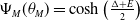 $\Psi _M(\theta _M )= \cosh \left ( \frac {\Delta + E }{2} \right )$
. Now notice that
$\Psi _M(\theta _M )= \cosh \left ( \frac {\Delta + E }{2} \right )$
. Now notice that
 $w_0- \cosh \left ( \frac {\Delta + E }{2} \right ) =e^\sigma - \alpha (e^E-1) (e^\Delta -1 )\gt 0$
because
$w_0- \cosh \left ( \frac {\Delta + E }{2} \right ) =e^\sigma - \alpha (e^E-1) (e^\Delta -1 )\gt 0$
because
 $\Delta \lt \Delta _c$
. Hence,
$\Delta \lt \Delta _c$
. Hence,
 $w_0 \gt \Phi (w_\theta ) + \theta \frac {E+ \Delta }{2}$
for every
$w_0 \gt \Phi (w_\theta ) + \theta \frac {E+ \Delta }{2}$
for every
 $\theta \gt 0$
. To prove (5.25), we only need to prove that
$\theta \gt 0$
. To prove (5.25), we only need to prove that
 $w_0 \gt \Phi (w_A) + \theta \frac {E+ \Delta }{2}$
for every
$w_0 \gt \Phi (w_A) + \theta \frac {E+ \Delta }{2}$
for every
 $\theta \gt 0$
. This is followed by the fact that
$\theta \gt 0$
. This is followed by the fact that
 \begin{equation*} \Phi (w_A)= w_A- \theta \frac {E+\Delta }{2} \end{equation*}
Hence
 $ \Phi (w_A)+ \theta \frac {E+\Delta }{2}=w_A \lt w_0$
.
$ \Phi (w_A)+ \theta \frac {E+\Delta }{2}=w_A \lt w_0$
.
Recall that
 $\Gamma \subset \{ w_A, w_S, w_0 \}$
is the set of the poles of the function
$\Gamma \subset \{ w_A, w_S, w_0 \}$
is the set of the poles of the function
 $f$
defined as in (5.22). The fact that equality (5.25) holds implies that the dominant term in
$f$
defined as in (5.22). The fact that equality (5.25) holds implies that the dominant term in
 $ n_{\tau \theta } = \ell _{\tau \theta } + h_{\tau \theta }$
is the leading term of
$ n_{\tau \theta } = \ell _{\tau \theta } + h_{\tau \theta }$
is the leading term of
 $\ell _{\tau \theta }$
which is (5.24). This implies that (5.18) holds.
$\ell _{\tau \theta }$
which is (5.24). This implies that (5.18) holds.
Theorem 5.9.
Let us define
 $\tau \,:\!=\, 2 \alpha e^{\frac {E+ \Delta }{2}} t$
and let
$\tau \,:\!=\, 2 \alpha e^{\frac {E+ \Delta }{2}} t$
and let
 $k\,:\!=\,\lfloor \theta \tau \rfloor$
for
$k\,:\!=\,\lfloor \theta \tau \rfloor$
for
 $\theta \geq 0$
. Assume that
$\theta \geq 0$
. Assume that
 $\Delta \gt \Delta _c$
.
$\Delta \gt \Delta _c$
.
-
1. If
$\theta$
is such that
$w_\theta \lt w_S$
, then we have that
(5.26)
\begin{equation} \lim _{t \to \infty } \frac { n_{k} (t) }{ e^{k({\log}(\varphi (\sigma ))- E ) } } = A(0) B(0) \overline n_S . \end{equation}
-
2. If instead
$\theta$
is such that
$w_\theta \gt w_S$
, then
(5.27)
\begin{equation} \lim _{t \to \infty } \frac { n_{k} (t) }{ e^{k({\log}(\varphi (\sqrt {1+\theta ^2 }))- E ) } } = 0. \end{equation}


Proof. As in the proof of Theorem5.8, we apply the inverse Laplace transform formula to deduce that
 \begin{equation*} n_k(t)= \frac {1}{2 \pi i } e^{- k E } \int _{\delta - i \infty }^{\delta + i \infty } e^{ zt } A(z) \hat {n}_S(z) \left ( 1+ B(z) \varphi (z)^k \right ) dz \end{equation*}
where
 $z_A \gt \delta \gt 0$
. As in the proof of Theorem5.8
$z_A \gt \delta \gt 0$
. As in the proof of Theorem5.8
 $n_k=\ell _k+ h_k$
where
$n_k=\ell _k+ h_k$
where
 \begin{equation} \ell _k (t)\,:\!=\, \frac {1}{2 \pi i } e^{- k E } \int _{\delta - i \infty }^{\delta + i \infty } e^{ zt } A(z) \hat {n}_S(z) dz = e^{- k E } \left ( A(0) \overline {n}_S + e^{ z_S t } A(z_S ) \frac {1}{z_S} \right ) \end{equation}
and
 \begin{equation} h_k (t)\,:\!=\, \frac {1}{2 \pi i } e^{- k E } \int _{\delta - i \infty }^{\delta + i \infty } e^{ zt } A(z) \hat {n}_S(z) B(z) \varphi (z)^k dz \end{equation}
Notice that since
 $ z_S \lt 0$
the dominant term in
$ z_S \lt 0$
the dominant term in
 $ \ell _k(t)$
as
$ \ell _k(t)$
as
 $t \rightarrow \infty$
is
$t \rightarrow \infty$
is
 $ e^{- k E } A(0) \overline {n}_S$
. Hence,
$ e^{- k E } A(0) \overline {n}_S$
. Hence,
 \begin{equation*} \ell _{\tau \theta } \left ( \frac {\tau }{ 2 \alpha e^{(E+\Delta )/2} }\right ) \sim e^{- \tau \theta E - \tau w_0 } e^{ \tau w_0 } A(0) \overline {n}_S \text{ as } \tau \to \infty . \end{equation*}
Moreover,
 \begin{align*} h_k(t)&= \frac {C(\alpha , E, \Delta )}{2 \pi i } e^{k \frac {\Delta - E }{2}}e^{- w_0 \tau }g_k(\tau ) \end{align*}
where
 $g_k$
and
$g_k$
and
 $C(\alpha , E, \Delta )$
are defined as in the proof of Theorem5.8. With the same arguments as the ones used in the proof of Theorem5.8, we deduce that
$C(\alpha , E, \Delta )$
are defined as in the proof of Theorem5.8. With the same arguments as the ones used in the proof of Theorem5.8, we deduce that
 \begin{equation*} g_{\tau \theta } (\tau ) \sim \int _{\gamma }f(w) dw - \frac { \sqrt {2\pi } i \theta a(w_\theta ) \tilde {n}_S(w_\theta )}{(\theta + \sqrt {1+ \theta ^2 } - e^{(E-\Delta )/2}) (1+\theta ^2)^{1/4}} \frac { e^{ \tau \Phi (w_\theta ) }}{\sqrt {\tau }} \text{ as } \tau \to \infty . \end{equation*}
where
 $\gamma$
is as in the proof of Theorem5.8. In order to compute
$\gamma$
is as in the proof of Theorem5.8. In order to compute
 $\int _{\gamma }f(w) dw$
, we need to distinguish between the following three cases.
$\int _{\gamma }f(w) dw$
, we need to distinguish between the following three cases.
-
1.
$w_0 \gt w_\theta \gt w_S$
, -
2.
$ w_0 \gt w_S \gt w_\theta$
, -
3.
$ w_\theta \gt w_0\gt w_S$
.


Case 1:
 $w_0 \gt w_\theta \gt w_S$
. Assume that 1. holds, hence that
$w_0 \gt w_\theta \gt w_S$
. Assume that 1. holds, hence that
 $\theta$
is such that
$\theta$
is such that
 $w_S \lt w_\theta \lt w_0$
. Then, we have that
$w_S \lt w_\theta \lt w_0$
. Then, we have that
 \begin{align*} \int _{\gamma }f(w) dw= 2 \pi i \operatorname {Res}_{w=w_0} f(w). \end{align*}
Now notice that
 \begin{equation*} \operatorname {Res}_{w=w_0} f(w) = \operatorname {Res}_{w=w_0} \tilde {n}_S (w) a(w_0) b(w_0) e^{\tau \Phi (w_0) } \end{equation*}
where we are using the notation
 \begin{equation*} b(w)\,:\!=\, \frac {1}{w+\sqrt {w^2-1}-e^{(E-\Delta )/2}} \end{equation*}
and where the function
 $a$
is given by (5.21) and the function
$a$
is given by (5.21) and the function
 $\Phi$
by (5.23). Therefore,
$\Phi$
by (5.23). Therefore,
 \begin{equation*} g_{\tau \theta } (\tau ) \sim \operatorname {Res}_{w=w_0} \tilde {n}_S (w) a(w_0) b(w_0) e^{\tau \Phi (w_0) } - \frac { \sqrt {2\pi } i \theta a(w_\theta ) \tilde {n}_S(w_\theta )}{(\theta + \sqrt {1+ \theta ^2 } - e^{(E-\Delta )/2}) (1+\theta ^2)^{1/4}} \frac { e^{ \tau \Phi (w_\theta ) }}{\sqrt {\tau }} \text{ as } \tau \to \infty . \end{equation*}
Hence
 \begin{align*} h_{\theta \tau } (t) \sim &C(\alpha , E, \Delta )e^{ - \theta \tau E - \tau w_0 } \Bigg[ b(w_0) a(w_0) e^{ \frac { \theta \tau (\Delta +E) }{2}} e^{\tau \Phi (w_0)} \operatorname {Res}_{w=w_0} \tilde {n}_S (w) \\[3pt] &- \frac { \theta b(w_\theta ) a(w_\theta ) \tilde {n}_S(w_\theta ) e^{ \tau \Phi (w_\theta ) + \tau \theta \frac {E+ \Delta }{2}} }{\sqrt {2 \pi \tau } (1+\theta ^2)^{1/4}} \Bigg] \text{ as } \tau \to \infty . \end{align*}
In order to study the behaviour of
 $n_{\theta \tau }(t)$
as
$n_{\theta \tau }(t)$
as
 $\tau \to \infty$
, we need to identify the leading order term in
$\tau \to \infty$
, we need to identify the leading order term in
 $\ell _{\theta \tau }+ h_{\theta \tau }$
. Since
$\ell _{\theta \tau }+ h_{\theta \tau }$
. Since
 $\Delta \gt \Delta _c$
and
$\Delta \gt \Delta _c$
and
 $w_0 \gt w_\theta$
, we have that
$w_0 \gt w_\theta$
, we have that
 \begin{equation*} \Phi (w_0) + \theta \frac {E+ \Delta }{2}=\max \left \{ w_0 , \Phi (w_0) + \theta \frac {E+ \Delta }{2}, \Phi (w_\theta ) + \theta \frac {E+ \Delta }{2} \right \}. \end{equation*}
Indeed, the fact that
 $\Delta \gt \Delta _c$
implies that
$\Delta \gt \Delta _c$
implies that
 \begin{equation*} \Phi (w_0) + \theta \frac {E+ \Delta }{2} \gt w_0 \gt w_S. \end{equation*}
Moreover, notice that by the definition of
 $w_\theta$
, we have that
$w_\theta$
, we have that
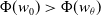 $\Phi (w_0) \gt \Phi (w_\theta )$
. Hence, the desired conclusion follows. We conclude that in this case
$\Phi (w_0) \gt \Phi (w_\theta )$
. Hence, the desired conclusion follows. We conclude that in this case
 \begin{equation} n_{\theta \tau } (t) \sim C(\alpha , \Delta , E) b(w_0) a(w_0) \operatorname {Res}_{w=w_0} \tilde {n}_S (w)e^{ \frac { \theta \tau (\Delta + E) }{2}} e^{\tau \Phi (w_0)} \text{ as } \tau \to \infty . \end{equation}
Therefore, using that
 \begin{equation*} C(\alpha , \Delta , E) b(w_0) a(w_0) \operatorname {Res}_{w=w_0} \tilde {n}_S (w)e^{ \frac { \theta \tau (\Delta + E) }{2}} e^{\tau \Phi (w_0)} = - A(0) B(0) \overline {n}_S \end{equation*}
we deduce that (5.26) holds.
Case 2:
 $w_0 \gt w_S \gt w_\theta$
. The main difference between case
$w_0 \gt w_S \gt w_\theta$
. The main difference between case
 $1$
and case
$1$
and case
 $2$
is the value of the integral
$2$
is the value of the integral
 $\int _\gamma f(w( dw )$
. Indeed, when
$\int _\gamma f(w( dw )$
. Indeed, when
 $\theta$
is such that
$\theta$
is such that
 $w_S \gt w_\theta$
, we have that
$w_S \gt w_\theta$
, we have that
 \begin{align*} \int _{\gamma } f(w) dw= 2 \pi i \left ( \operatorname {Res}_{w=w_0} f(w)+ \operatorname {Res}_{w=w_S} f(w) \right ) . \end{align*}
As a consequence, computations similar to the ones made for case 1 imply that
 \begin{align*} h_{\theta \tau } (t)\sim &e^{ - \theta \tau E - \tau w_0 } \Bigg[ b(w_0) \operatorname {Res}_{w=w_0} \tilde {n}_S (w) e^{ \frac { \theta \tau (\Delta - E) }{2}} e^{\tau \Phi (w_0)} +b(w_S) \operatorname {Res}_{n=n_S} \left (\tilde {n}_S (w ) \right ) e^{ \frac { \theta \tau (\Delta - E) }{2}} e^{\tau \Phi (w_S)} \\ & - \frac { \theta b(w_\theta ) a(w_\theta ) \tilde {n}_S(w_\theta )}{\sqrt {2 \pi } (1+\theta ^2)^{1/4}} \frac { e^{ \tau \Phi (w_\theta ) + \tau \theta \frac {E+ \Delta }{2}}}{\sqrt {\tau }}\Bigg]. \end{align*}
In order to find the leading order term in
 $\ell _{\theta \tau } + h_{\theta \tau }$
, we prove that
$\ell _{\theta \tau } + h_{\theta \tau }$
, we prove that
 \begin{equation} \Phi (w_0) + \theta \frac {E+ \Delta }{2}=\max \left \{ w_0 , \Phi (w_0) + \theta \frac {E+ \Delta }{2}, \Phi (w_\theta ) + \theta \frac {E+ \Delta }{2}, \Phi (w_S) + \theta \frac {E+ \Delta }{2} \right \}. \end{equation}
Indeed, the fact that
 $\Delta \gt \Delta _c$
implies that
$\Delta \gt \Delta _c$
implies that
 \begin{equation*} \Phi (w_0) +\theta \frac {E+ \Delta }{2} \gt w_0 \gt w_S \gt \Phi (w_s) \text{ and } \Phi (w_0)\gt \Phi (w_\theta ). \end{equation*}
Therefore, the asymptotics (5.26) follow.
Case 3:
 $w_\theta \gt w_0 \gt w_S$
. When
$w_\theta \gt w_0 \gt w_S$
. When
 $\theta$
is such that
$\theta$
is such that
 $ w_\theta \gt w_0 \gt w_S$
, we have that
$ w_\theta \gt w_0 \gt w_S$
, we have that
 \begin{align*} \int _{\gamma } f(w) dw= 0. \end{align*}
As a consequence,
 \begin{align*} h_{\theta \tau } (t)\sim - \frac { C(\alpha , E, \Delta ) \theta b(w_\theta ) a(w_\theta ) \tilde {n}_S(w_\theta )}{\sqrt {2 \pi } (1+\theta ^2)^{1/4}} \frac { e^{ \tau \Phi (w_\theta ) + \tau \theta \frac {E+ \Delta }{2}}}{\sqrt {\tau }} \text{ as } \tau \to \infty . \end{align*}
Notice that the fact that
 $ w_\theta \gt w_0 \gt w_S$
and
$ w_\theta \gt w_0 \gt w_S$
and
 $\Delta \gt \Delta _c$
imply that
$\Delta \gt \Delta _c$
imply that
 \begin{equation*} \Phi (w_\theta ) + \theta \frac {E+ \Delta }{2} =\max \left \{ w_0 , \Phi (w_\theta ) + \theta \frac {E+ \Delta }{2} \right \}. \end{equation*}
Hence,
 \begin{equation*} n_{\theta \tau } (t)\sim - \frac { C(\alpha , E, \Delta ) \theta b(w_\theta ) a(w_\theta ) \tilde {n}_S(w_\theta )}{\sqrt {2 \pi } (1+\theta ^2)^{1/4}} \frac { e^{ \tau \Phi (w_\theta ) + \tau \theta \frac {E+ \Delta }{2}}}{\sqrt {\tau }} \text{ as } \tau \to \infty \text{ as } \tau \to \infty \end{equation*}
Therefore, (5.27) follows.
Theorem 5.10.
Let us define
 $\tau \,:\!=\, 2 \alpha e^{\frac {E+ \Delta }{2}} t$
and let
$\tau \,:\!=\, 2 \alpha e^{\frac {E+ \Delta }{2}} t$
and let
 $k\,:\!=\,\lfloor \theta \tau \rfloor$
for
$k\,:\!=\,\lfloor \theta \tau \rfloor$
for
 $\theta \geq 0$
.
$\theta \geq 0$
.
Assume that
 $\Delta = \Delta _c$
. Then,
$\Delta = \Delta _c$
. Then,
-
1. if
$\theta$
is such that
$w_\theta \lt w_S$
, then we have that
(5.32)
\begin{equation} \lim _{t \to \infty } \frac { n_{k} (t) }{ e^{- k E } } = \overline n_S \left ( 1- \frac {1}{2\alpha e^E}\right ). \end{equation}
-
2. If instead
$\theta$
is such that
$w_\theta \gt w_S$
, then
(5.33)
\begin{equation} \lim _{t \to \infty } \frac { n_{k} (t) }{ e^{k({\log} (\varphi (w_\theta ))- E ) } } = 0. \end{equation}


Proof. Notice that if
 $\Delta = \Delta _c$
, we have that
$\Delta = \Delta _c$
, we have that
 $z_A=z_0$
and as a consequence we have that
$z_A=z_0$
and as a consequence we have that
 \begin{equation*} w_0=w_A= \cosh\! (E). \end{equation*}
As in the proof of Theorem5.8 and Theorem5.9, we deduce that the function
 $\ell _k$
defined as in (5.28) is given by
$\ell _k$
defined as in (5.28) is given by
 \begin{equation*} \ell _{\tau \theta }(t)\sim e^{- \tau \theta E - w_0 \tau } e^{ w_0 \tau } \overline n_S \text{ as } \tau \to \infty . \end{equation*}
In order to obtain the asymptotics of
 $n_{k}$
, we have to compute the asymptotics of the function
$n_{k}$
, we have to compute the asymptotics of the function
 $h_{\theta \tau } (\tau )= \frac {C(\alpha , E, \Delta )}{2 \pi i } e^{- w_0 \tau }g_{\tau \theta } (\tau )$
where
$h_{\theta \tau } (\tau )= \frac {C(\alpha , E, \Delta )}{2 \pi i } e^{- w_0 \tau }g_{\tau \theta } (\tau )$
where
 \begin{align*} g_{\tau \theta } (\tau )= \int _{\gamma } f(w) dw - \int _{\gamma _2} f(w) dw \end{align*}
where
 $\gamma$
and
$\gamma$
and
 $\gamma _2$
are defined as in Theorem5.10, and
$\gamma _2$
are defined as in Theorem5.10, and
 $f$
is given by (5.22).
$f$
is given by (5.22).
When
 $w_0 \gt w_\theta \gt w_S$
, then
$w_0 \gt w_\theta \gt w_S$
, then
 \begin{equation*} \int _{\gamma } f(w) dw = 2 \pi i \left [ \operatorname {Res}_{ w =w_0} f(w) \right ] = 2 \pi i e^{\tau \Phi _0} \frac {b(w_0) \overline n_S }{(2 \alpha )^2 e^{2E} } = 2 \pi i e^{\tau (w_0- \theta E)} \frac {b(w_0) \overline n_S }{(2 \alpha )^2 e^{2E} }. \end{equation*}
where we are using the fact that
 $\Phi (w_0)=w_0 - \theta E.$
This together with detailed asymptotics of
$\Phi (w_0)=w_0 - \theta E.$
This together with detailed asymptotics of
 $\int _{\gamma _2} f(w) dw$
as
$\int _{\gamma _2} f(w) dw$
as
 $\tau \rightarrow \infty$
implies that as
$\tau \rightarrow \infty$
implies that as
 $\tau \to \infty$
 \begin{align*} g_{\tau \theta } \sim 2 \pi i e^{\tau (w_0- \theta E)} \frac {b(w_0) \overline n_S }{(2 \alpha )^2 e^{2E} } - \frac { \theta \sqrt {2 \pi } i a(w_\theta ) \tilde {n}_S(w_\theta )}{(\theta + \sqrt {1+ \theta ^2 } - 1) (1+\theta ^2)^{1/4}} \frac { e^{ \tau \Phi (w_\theta ) }}{\sqrt {\tau }}. \end{align*}
Moreover, notice that
 \begin{equation*} w_0= \max _{\theta \gt 0} \left (\Phi (w_\theta ) + \theta E \right ). \end{equation*}
and we recall that the maximum of the function
 $\Psi _M = \Phi (w_\theta ) + \theta E$
is attained at
$\Psi _M = \Phi (w_\theta ) + \theta E$
is attained at
 $\theta _M = \sinh\! (E)$
, hence when
$\theta _M = \sinh\! (E)$
, hence when
 $w_\theta = \sqrt {1+ \theta _M^2 } = \cosh\! (E)= w_0$
. Therefore, when
$w_\theta = \sqrt {1+ \theta _M^2 } = \cosh\! (E)= w_0$
. Therefore, when
 $w_0\gt w_\theta$
, we have that
$w_0\gt w_\theta$
, we have that
 \begin{align*} g_{\tau \theta } \sim 2 \pi i e^{\tau (w_0- \theta E)} \frac {b(w_0) \overline n_S }{(2 \alpha )^2 e^{2E} } =2 \pi i e^{\tau (w_0- \theta E)} \frac { \overline n_S }{(2 \alpha )^2 e^{2E} (e^E-1)} . \end{align*}
As a consequence, we deduce that
 \begin{equation} n_{\tau \theta } (t) \sim e^{- \tau \theta E }\overline n_S \left ( 1- \frac {1 }{2 \alpha e^{E} } \right ) \text{ as } \tau \to \infty , \end{equation}
where we used the fact that
 $C(\alpha , E, E)= 2 \alpha (e^{2E} - e^E )$
. When
$C(\alpha , E, E)= 2 \alpha (e^{2E} - e^E )$
. When
 $w_0 = w_\theta \gt w_S$
, we obtain the same result. When
$w_0 = w_\theta \gt w_S$
, we obtain the same result. When
 $ w_0 \gt w_S \gt w_\theta$
, then we have that
$ w_0 \gt w_S \gt w_\theta$
, then we have that
 \begin{equation*} \int _{\gamma } f(w) dw = 2 \pi i \left [ \operatorname {Res}_{ w =w_0} f(w) + \operatorname {Res}_{ w =w_S} f(w) \right ] \end{equation*}
and we can prove that (5.34) holds also in this case.
Finally, when
 $ w_\theta \gt w_0\gt w_S$
, then
$ w_\theta \gt w_0\gt w_S$
, then
 \begin{equation*} \int _{\gamma } f(w) dw = 0. \end{equation*}
This implies (5.33).
6. Analysis of the model with a finite number of kinetic proofreading steps
In this section, we study in detail, using Laplace transforms, the model described by (2.4) when the number of kinetic proofreading steps
 $N$
is large, but finite. We recover the same results obtained using matched asymptotics expansions in Section 4.
$N$
is large, but finite. We recover the same results obtained using matched asymptotics expansions in Section 4.
Performing the Laplace transform to all the terms in equation (2.4), we obtain the following equation for the vector of the Laplace transforms
 $(\hat {n}_S, \hat {n}_0, \ldots , \hat {n}_{N})$
of the concentrations
$(\hat {n}_S, \hat {n}_0, \ldots , \hat {n}_{N})$
of the concentrations
 $(n_S, n_0, \ldots , n_{N})$
 \begin{align} \left ( z + \frac {{1- e^{- N E} }}{1- e^{-E}} + \mu + e^\sigma \right ) \hat {n}_S(z)&= 1+ e^\sigma \hat {M}(z)\nonumber \\ \left ( z + e^\sigma + \alpha e^\Delta + \mu \right ) \hat {n}_0 (z)&= \hat {n}_S(z) + \alpha e^E \hat {n}_1 (z)\nonumber \\ \Omega (z) \hat {n}_k(z)&= e^{- k E} \hat {n}_S (z)+ \alpha e^E\hat {n}_{k+1} (z)+ \alpha e^\Delta \hat {n}_{k-1}(z), \ k \in \{1, \ldots , N\} \nonumber \\ n_{N+1}(z)&=0 \end{align}
where
 $\Omega (z)$
is defined as (5.3) and where
$\Omega (z)$
is defined as (5.3) and where
 \begin{equation*} \hat {M}(z)= \sum _{k=0}^{N } \hat {n}_k (z) + \hat {n}_S(z) . \end{equation*}
Since the probability of response is given by
 \begin{equation*} p_{res}(\sigma ) = \alpha e^\Delta \hat {n}_N(0) \end{equation*}
we aim at studying the behaviour of
 $\hat {n}_N (0)$
as
$\hat {n}_N (0)$
as
 $N \to \infty$
. Using computations that are similar to the ones of Proposition 5.6, we prove the following Lemma.
$N \to \infty$
. Using computations that are similar to the ones of Proposition 5.6, we prove the following Lemma.
Lemma 6.1.
Assume that
 $\hat {n}_S(0) \in \mathbb R_*$
and
$\hat {n}_S(0) \in \mathbb R_*$
and
 $\hat {n}_0 (0)$
are given. Let
$\hat {n}_0 (0)$
are given. Let
 $\{ \hat {n}_k (0) \}_{k =1}^N$
be the sequence of
$\{ \hat {n}_k (0) \}_{k =1}^N$
be the sequence of
 $\hat {n}_k(0)$
defined as
$\hat {n}_k(0)$
defined as
 \begin{equation} \hat {n}_k (0) = e^{- k E } \left[A(0) \hat {n}_S(0) + F_1(N) \varphi (\sigma )^k +F_2 (N) \varphi _2^k \right], \quad 1 \leq k \leq N \end{equation}
where
 \begin{equation*} \varphi _2= \frac {1}{2 \alpha } \left ( \Omega (0) + \sqrt {\Omega (0)^2 - 4 \alpha ^2 e^{E+\Delta }} \right ) \end{equation*}
and where
 \begin{equation} F_1(N)\,:\!=\, \frac {A(0) \hat {n}_S(0) + (\hat {n}_0 (0)- A(0) \hat {n}_S (0)) \varphi _2^{N+1} }{\varphi _2^{N+1} -\varphi (\sigma )^{N+1} }, \quad F_2(N)\,:\!=\, \frac {A(0) \hat {n}_S(0) + (\hat {n}_0(0) - A(0) \hat {n}_S (0)) \varphi (\sigma )^{N+1} }{\varphi (\sigma ) ^{N+1} -\varphi _2^{N+1} }. \end{equation}
The vector
 $ ( \hat {n}_S(0), \hat {n}_0(0), \hat {n}_1(0) , \ldots \hat {n} _{N} (0) )$
satisfies
$ ( \hat {n}_S(0), \hat {n}_0(0), \hat {n}_1(0) , \ldots \hat {n} _{N} (0) )$
satisfies
 \begin{align*} \Omega (0) \hat {n}_k(0)&= e^{- k E} \hat {n}_S (0)+ \alpha e^E\hat {n}_{k+1} (0)+ \alpha e^\Delta \hat {n}_{k-1}(0), \ k \in \{1, \ldots , N\} \\ n_{N+1}(0)&=0 \end{align*}
As a consequence, enforcing that
 $\hat {n}_S(0)$
satisfies
$\hat {n}_S(0)$
satisfies
 $ \left ( \frac {{1- e^{- N E} }}{1- e^{-E}} + \mu + e^\sigma \right ) \hat {n}_S(0)= 1+ e^\sigma \hat {M}(0)$
, we can prove the following Lemma.
$ \left ( \frac {{1- e^{- N E} }}{1- e^{-E}} + \mu + e^\sigma \right ) \hat {n}_S(0)= 1+ e^\sigma \hat {M}(0)$
, we can prove the following Lemma.
Lemma 6.2.
Assume that
 $\hat {n}_0(0) \in \mathbb R_*$
is given by
$\hat {n}_0(0) \in \mathbb R_*$
is given by
 \begin{equation*} \hat {n}_0 (0) =G_N \hat {n}_S(0) \end{equation*}
with
 \begin{equation*} G_N = \frac {1+ \alpha A +\alpha A \left ( \frac { \varphi (\sigma ) - \varphi _2 }{ \varphi _2^{N+1} - (\varphi (\sigma ))^{N+1}}- \Psi _N \right ) }{ e^\sigma + \alpha e^\Delta + \mu -\alpha \Psi _N} \ \text{ where } \ \Psi _N = \frac {\varphi _2^{N+1} \varphi (\sigma )-(\varphi (\sigma ))^{N+1} \varphi _2 }{ \varphi _2^{N+1} - (\varphi (\sigma ))^{N+1}} \end{equation*}
Assume that
 $\hat {n}_S(0) \in \mathbb R_*$
is given by
$\hat {n}_S(0) \in \mathbb R_*$
is given by
 \begin{equation*} \hat {n}_S (0)= \frac {{1- e^{- N E} }}{1- e^{-E}} + \mu + e^\sigma C_N \end{equation*}
where
 \begin{align*} C_N\,:\!=\, \left (\! 1- A(0) \frac { {1- e^{- N E} } }{1- e^{-E}} -\frac { A(0) + (G_N- A(0) ) \varphi (\sigma )^N }{\varphi _2^{N+1} - \varphi (\sigma )^{N+1}} \frac {\varphi (\sigma )^{- N } -1 }{1- \varphi (\sigma ) }- \frac { A(0) + (G_N{-} A(0) ) \varphi _2^N }{\varphi (\sigma )^{N+1} - \varphi _2^{N+1}} \frac {\varphi _2^{- N } {-}1 }{1- \varphi _2}\right )\!. \end{align*}
Assume that the vector
 $( \hat {n}_0 (0) , \hat {n}_1 (0), \ldots , \hat {n}_N (0) )$
is defined as in Lemma 6.1
. Then,
$( \hat {n}_0 (0) , \hat {n}_1 (0), \ldots , \hat {n}_N (0) )$
is defined as in Lemma 6.1
. Then,
 $( \hat {n}_S (0) , \hat {n}_0 (0), \hat {n}_1 (0), \ldots , \hat {n}_N (0) )$
is the unique solution to
$( \hat {n}_S (0) , \hat {n}_0 (0), \hat {n}_1 (0), \ldots , \hat {n}_N (0) )$
is the unique solution to
 \begin{align*} \left ( \frac { {1- e^{- N E} } }{1- e^{-E}} + \mu + e^\sigma \right ) \hat {n}_S(0)&= 1+ e^\sigma \hat {M}(0) \\ ( e^\sigma + \alpha e^\Delta + \mu ) \hat {n}_0 (0)&= \hat {n}_S(0) + \alpha e^E \hat {n}_1 (0) \\ \Omega (0) \hat {n}_k(0)&= e^{- k E} \hat {n}_S (0)+ \alpha e^E\hat {n}_{k+1} (0)+ \alpha 0e^\Delta \hat {n}_{k-1}(0), \ k \in \{1, \ldots , N\} \\ n_{N+1}(0)&=0 \end{align*}
Lemma 6.3.
Let
 $F_1(N)$
and
$F_1(N)$
and
 $F_2(N)$
be given by (6.3). Then, we have
$F_2(N)$
be given by (6.3). Then, we have
 \begin{equation*} F_1(N) \sim \hat {n}_0 (0) - A(0)\hat {n}_S(0) \ \text{ as } N \to \infty \end{equation*}
and
 \begin{equation*} F_2(N) \sim - \frac { A(0) \hat {n}_S(0) + (\hat {n_0} (0) - A(0)\hat {n}_S(0) ) \varphi (\sigma )^{N+1}}{\varphi _2^{N+1}} \ \text{ as } N \to \infty . \end{equation*}
Proof. In order to prove this Lemma, it is enough to notice that Lemma 5.4 implies that
 $\varphi (\sigma ) \lt \varphi _2$
.
$\varphi (\sigma ) \lt \varphi _2$
.
Proposition 6.4.
Assume that
 $\hat {n}_N (0)$
is as in Lemma 6.2
. Then, we have that
$\hat {n}_N (0)$
is as in Lemma 6.2
. Then, we have that
-
• if
$\Delta \lt \Delta _c$
, then
\begin{equation*} \hat {n}_N (0) \sim \overline {n}_S \hat {M}(0) e^{- N E } A(0) \left ( 1- \frac {1}{\varphi _2 }\right ) \text{ as } N \to \infty . \end{equation*}
-
• If
$\Delta \gt \Delta _c$
, then
where we recall that
\begin{equation*} \hat {n}_N (0) \sim \overline {n}_S \hat {M}(0) e^{- N [E + \log (\varphi (\sigma ) ) ] } (G- A(0) ) \left ( 1- \frac {\varphi (\sigma ) }{ \varphi _2}\right ) \text{ as } N \to \infty \end{equation*}
$G$
is given by (6.2).


Proof. Lemma 6.3 together with Lemma 6.2 imply that
 \begin{equation*} \hat {n}_1 (0) =e^{-E } ( A(0) \hat {n}_S (0)+ F_1 \varphi (\sigma ) + F_2 \varphi _2) \sim e^{-E } ( A(0) \hat {n}_S (0) + (\hat {n}_0(0) - A(0) \hat {n}_S )\varphi (\sigma ) ). \end{equation*}
Using the asymptotics for
 $\hat {n}_1$
, we deduce that
$\hat {n}_1$
, we deduce that
 \begin{equation*} \hat {n}_0 (0)= \frac {\hat {n}_S + \alpha e^E \hat {n}_1(0)}{\mu + \alpha e^\Delta + e^\sigma } \sim \frac {\hat {n}_S + \alpha ( A(0) \hat {n}_S + (\hat {n}_0 - A(0) \hat {n}_S )\varphi (\sigma ) ) }{ \alpha e^\Delta + e^\sigma } \end{equation*}
Hence,
 $\hat {n}_0(0) \sim G \hat {n}_S$
where
$\hat {n}_0(0) \sim G \hat {n}_S$
where
 \begin{equation} G= \frac {1+ \alpha A(0) (1- \varphi (\sigma ) )}{ e^\sigma + \alpha e^\Delta - \alpha \varphi (\sigma )}. \end{equation}
Using the asymptotics for
 $\hat {n}_0(0)$
as well as the fact that
$\hat {n}_0(0)$
as well as the fact that
 $n_N (0)$
is given by (6.2), we obtain that
$n_N (0)$
is given by (6.2), we obtain that
 \begin{equation*} \hat {n}_N (0) \sim \hat {n}_S (0) e^{- N E } \left ( A(0) \left ( 1- \frac {1}{\varphi _2 }\right ) + (G- A(0) ) \left ( 1- \frac {\varphi (\sigma ) }{ \varphi _2}\right ) \varphi (\sigma )^N \right ) \text{ as } N \to \infty . \end{equation*}
The fact that
 \begin{equation*} \frac {dM}{dt } =- \alpha e^\Delta n_{N} - \mu M \end{equation*}
implies that
 \begin{equation*} \hat {M}(0) =\frac { 1 - \alpha e^\Delta \hat {n}_{N}(0)}{\mu } \sim \frac {1}{\mu }. \end{equation*}
As a consequence, we have that
 $\hat {n}_S(0) \sim \overline n_S \hat {M}(0)$
as
$\hat {n}_S(0) \sim \overline n_S \hat {M}(0)$
as
 $N \to \infty$
. This, combined with the fact that when
$N \to \infty$
. This, combined with the fact that when
 $\Delta \lt \Delta _c$
we have that
$\Delta \lt \Delta _c$
we have that
 $\varphi (\sigma ) \lt 1$
while when
$\varphi (\sigma ) \lt 1$
while when
 $\Delta \gt \Delta _c$
we have that
$\Delta \gt \Delta _c$
we have that
 $\varphi (\sigma ) \gt 1$
to obtain the desired result.
$\varphi (\sigma ) \gt 1$
to obtain the desired result.
Theorem 6.5.
Let
 $p_{res} (\sigma )$
be the probability of response defined by (2.7). Then we have that
$p_{res} (\sigma )$
be the probability of response defined by (2.7). Then we have that
-
• if
$\Delta \lt \Delta _c$
, then
where
\begin{equation*} p_{res}(\sigma ) \sim \left ( 1 + C_1 e^{N(E- b)} \right )^{-1} \text{ as } N \to \infty \end{equation*}
$C_1\,:\!=\,\left [ \alpha e^{\Delta } A(0) \overline n_S \left (1- \varphi (\sigma ) e^{-(E + \Delta )} \right ) \right ]^{-1}$
.
-
• if instead
$\Delta \gt \Delta _c$
, then we have that
where
\begin{equation*} p_{res} (\sigma ) \sim \left ( 1 + C_2 e^{N(E- b - \log (\varphi (\sigma ))} \right )^{-1} \text{ as } N \to \infty \end{equation*}
\begin{equation*} C_2= \left (\overline {n}_S \alpha e^\Delta (G- A(0) ) \left ( 1-(\varphi (\sigma ))^2 e^{- (\Delta + E)}\right ) \right )^{-1} . \end{equation*}


Proof. Recall that
 \begin{equation} \hat {M} (0)= \frac {1 - \alpha e^\Delta \hat {n}_{N} (0) }{\mu }. \end{equation}
Plugging
 $\hat {M}(0)$
in the asymptotics for
$\hat {M}(0)$
in the asymptotics for
 $\hat {n}_N(0)$
and using the fact that
$\hat {n}_N(0)$
and using the fact that
 $\frac { 1}{\varphi _2} = \varphi (\sigma ) e^{- (E+ \Delta )}$
, we obtain the desired conclusions.
$\frac { 1}{\varphi _2} = \varphi (\sigma ) e^{- (E+ \Delta )}$
, we obtain the desired conclusions.
The constants
 $C_1$
and
$C_1$
and
 $C_2$
in Theorem6.5 are the same constants that we obtained using matched asymptotics, i.e. (4.26) and (4.27). (In order to see that the constant
$C_2$
in Theorem6.5 are the same constants that we obtained using matched asymptotics, i.e. (4.26) and (4.27). (In order to see that the constant
 $C_2$
is the same constant that appears in (4.27), notice that
$C_2$
is the same constant that appears in (4.27), notice that
 $G-A(0)= B A(0)$
where
$G-A(0)= B A(0)$
where
 $B$
is given by (4.9).)
$B$
is given by (4.9).)

7. Some PDE limits
In this section, we derive two PDEs that can be seen as an approximation of the discrete model (2.4) as
 $N \to \infty$
in different parameter regimes. These PDEs are particular types of renewal equations (see, for instance, [Reference Perthame27]) and can be analysed with computations that are simpler compared to the ones of Section 6.
$N \to \infty$
in different parameter regimes. These PDEs are particular types of renewal equations (see, for instance, [Reference Perthame27]) and can be analysed with computations that are simpler compared to the ones of Section 6.
When
 $e^\sigma \approx \frac {1}{N }$
and
$e^\sigma \approx \frac {1}{N }$
and
 $\Delta \gt E$
and both
$\Delta \gt E$
and both
 $E$
and
$E$
and
 $\Delta$
are of order one, we will derive the following PDE
$\Delta$
are of order one, we will derive the following PDE
 \begin{align} \partial _\tau f(\tau ,x) &= - \beta f(\tau ,x) + \alpha \left ( e^E- e^\Delta \right ) \partial _x f(\tau ,x) - \delta f(\tau ,x), \quad x \in (0,L)\\[-10pt]\nonumber \end{align}
 \begin{align} f(\tau , 0) & = \frac {\beta }{\alpha ( e^\Delta - e^E ) }\int _0^L f(\tau , x) dx, \end{align}
for a suitable
 $\beta \gt 0$
,
$\beta \gt 0$
,
 $\delta \gt 0$
, and
$\delta \gt 0$
, and
 $L\gt 1$
and initial condition
$L\gt 1$
and initial condition
 \begin{equation} \int _0^L f(0, x ) dx =1. \end{equation}
The steady states of the equation above behave as
 $ e^{-\lambda x }$
where
$ e^{-\lambda x }$
where
 $\lambda = \frac {\beta + \delta }{ \alpha (e^\Delta - e^E) }$
. Since
$\lambda = \frac {\beta + \delta }{ \alpha (e^\Delta - e^E) }$
. Since
 $\lambda$
depends non trivially on
$\lambda$
depends non trivially on
 $\beta$
, the model has strong discrimination properties. Notice that this is expected as in this regime, we have that
$\beta$
, the model has strong discrimination properties. Notice that this is expected as in this regime, we have that
 \begin{equation*} \Delta _c = \log \left ( 1 + \frac { \beta }{ N \alpha (e^E-1) } \right ) \sim \frac { \beta }{ N \alpha (e^E-1) } \text{ as } N \to \infty . \end{equation*}
Instead, when we assume that
 $e^\sigma \approx \frac {1}{N }$
and
$e^\sigma \approx \frac {1}{N }$
and
 $\Delta \approx 1$
and
$\Delta \approx 1$
and
 $E\approx \frac {1}{N }$
, we derive the following PDE
$E\approx \frac {1}{N }$
, we derive the following PDE
 \begin{align} \partial _\tau f (\tau ,x) =& e^{- x } m (\tau ) - \beta f(\tau , x) {+ } \alpha (1-e^\Delta ) \partial _x f (\tau ,x) - \delta f(\tau ,x)\\[-10pt]\nonumber \end{align}
 \begin{align} m(\tau ) =& \frac {\beta }{1-e^{-L}} \int _0^L f(\tau , x) dx\\[-10pt]\nonumber \end{align}
 \begin{align} f(\tau , 0)=& 0. \end{align}
If we ignore the loss term
 $- \delta f$
, the steady states of this equation have the form
$- \delta f$
, the steady states of this equation have the form
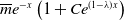 $ \overline m e^{- x } \left ( 1+ C e^{ (1- \lambda ) x} \right )$
for a suitable constants
$ \overline m e^{- x } \left ( 1+ C e^{ (1- \lambda ) x} \right )$
for a suitable constants
 $\overline m$
and
$\overline m$
and
 $C$
and for
$C$
and for
 $\lambda = \frac {\beta }{ \alpha (e^\Delta -1) }$
. Notice that in order to have strong discrimination properties in this case, we need to assume that
$\lambda = \frac {\beta }{ \alpha (e^\Delta -1) }$
. Notice that in order to have strong discrimination properties in this case, we need to assume that
 \begin{equation*} e^\Delta \gt 1+ \frac { \beta }{ \alpha }. \end{equation*}
This condition is expected; indeed, in this regime, we have that
 \begin{equation*} e^{\Delta _c} = 1 + \frac {e^\sigma }{ \alpha (e^E -1 )} = 1 + \frac {\beta }{ N \alpha (e^{1/N} -1 )} \sim 1+ \frac { \beta }{ \alpha } \text{ as } N \to \infty . \end{equation*}
Notice that in order to obtain the PDEs above as an approximation of the discrete system (2.4), we have to assume that
 $\Delta \gt E$
. The two PDEs that we obtain have a transport term that has a sign, in particular in both the cases we have a transport of complexes toward larger phosphorylation states, i.e. to larger
$\Delta \gt E$
. The two PDEs that we obtain have a transport term that has a sign, in particular in both the cases we have a transport of complexes toward larger phosphorylation states, i.e. to larger
 $k$
. However, we can have situations in which detailed balance fails with
$k$
. However, we can have situations in which detailed balance fails with
 $\Delta \gt \Delta _c$
, but in which the PDE approximation is not valid because
$\Delta \gt \Delta _c$
, but in which the PDE approximation is not valid because
 $E \gt \Delta \gt \Delta _c$
. In these cases, the discrete model (2.4) cannot be approximated with a PDE, and the transport towards small
$E \gt \Delta \gt \Delta _c$
. In these cases, the discrete model (2.4) cannot be approximated with a PDE, and the transport towards small
 $k$
dominates the transport towards large
$k$
dominates the transport towards large
 $k$
.
$k$
.
7.1. PDE limit when
$E\approx 1$
,
$\Delta \approx 1$
,
$\Delta \gt E$
,
$e^\sigma \approx \frac {1}{N}$
, and
$\mu \approx \frac {1}{N}$


In this section, we assume that the number of kinetic proofreading steps is
 $L N$
where
$L N$
where
 $L \gt 1$
and where
$L \gt 1$
and where
 $N$
tends to infinity. In order to derive equation (7.1), let us consider the behaviour of the solution to (2.4) when
$N$
tends to infinity. In order to derive equation (7.1), let us consider the behaviour of the solution to (2.4) when
 $k \approx N$
and when
$k \approx N$
and when
 $k \approx 1$
under the assumption that
$k \approx 1$
under the assumption that
 $E\approx 1$
,
$E\approx 1$
,
 $\Delta \approx 1$
,
$\Delta \approx 1$
,
 $\Delta \gt E$
, and
$\Delta \gt E$
, and
 $e^\sigma \approx \frac {1}{N}$
,
$e^\sigma \approx \frac {1}{N}$
,
 $\mu \approx \frac {1}{N}$
.
$\mu \approx \frac {1}{N}$
.
Behaviour of
 $\boldsymbol{n_k}$
for
$\boldsymbol{n_k}$
for
 $\boldsymbol{k \approx N}$
. Let us assume that
$\boldsymbol{k \approx N}$
. Let us assume that
 $e^\sigma N = \beta \gt 0$
and that
$e^\sigma N = \beta \gt 0$
and that
 $\mu N=\delta \gt 0$
. Notice that (2.4) implies that
$\mu N=\delta \gt 0$
. Notice that (2.4) implies that
 \begin{equation*} \partial _t n_k = n_S e^{- k E } - e^\sigma n_k + \alpha (e^E- e^\Delta ) (n_{k-1} - n_k ) + \alpha e^\Delta (n_{k+1 } - 2 n_k + n_{k-1} )- \mu n_k \end{equation*}
where
 \begin{equation*} \partial _t n_S = - \left ( 1 + e^{- E } \frac {1- e^{- N L E }}{1- e^{- E }} \right ) n_S + e^{\sigma } \sum _{k=0}^{N L} n_k - \mu n_S \end{equation*}
We now define
 $x= \frac {k}{N }$
,
$x= \frac {k}{N }$
,
 $\tau = \frac {t }{ N }$
,
$\tau = \frac {t }{ N }$
,
 $f(\tau , x)= N n_k(t)$
, and
$f(\tau , x)= N n_k(t)$
, and
 $m(\tau )= N n_S (t)$
.
$m(\tau )= N n_S (t)$
.
We deduce that
 $f$
and
$f$
and
 $m$
satisfy the following system of equations
$m$
satisfy the following system of equations
 \begin{align*} \partial _\tau f (\tau ,x) & = N e^{- E x N } m (\tau ) - e^\sigma N f(\tau , x) + \alpha (e^E - e^\Delta ) N \left [ f\left (\tau , x- \frac {1}{N } \right ) - f(\tau , x) \right ] \\[3pt] & \quad + \alpha e^\Delta N \left [ f\left (\tau , x+\frac {1}{N } \right ) - f(\tau , x) + f\left (\tau , x-\frac {1}{N } \right ) \right ] - N \mu f(\tau ,x) \\[3pt] \frac {1}{N} \partial _\tau m(\tau ) &= e^\sigma \sum _{k=0}^{NL} f \left (\tau , \frac {k}{N} \right ) - \left ( 1 + e^{- E } \frac {1- e^{- N L E }}{1- e^{- E }} \right ) m(\tau ) - \mu m(\tau ). \end{align*}
Using the fact that
 $e^\sigma N = \beta$
and that
$e^\sigma N = \beta$
and that
 $\mu N=\delta$
and the fact that
$\mu N=\delta$
and the fact that
 $ N \left [ f\left (\tau , x- \frac {1}{N } \right ) - f(\tau , x) \right ] \approx \partial _x f(\tau ,x)$
as
$ N \left [ f\left (\tau , x- \frac {1}{N } \right ) - f(\tau , x) \right ] \approx \partial _x f(\tau ,x)$
as
 $N \to \infty$
as well as the fact that
$N \to \infty$
as well as the fact that
 $N \left [ f\left (\tau ,x+\frac {1}{N } \right ) - f(\tau , x) + f\left (\tau , x-\frac {1}{N } \right ) \right ] \approx \frac {1}{N} \partial ^2_{xx}\, f(\tau ,x) \approx 0$
as
$N \left [ f\left (\tau ,x+\frac {1}{N } \right ) - f(\tau , x) + f\left (\tau , x-\frac {1}{N } \right ) \right ] \approx \frac {1}{N} \partial ^2_{xx}\, f(\tau ,x) \approx 0$
as
 $N \to \infty$
, we deduce that
$N \to \infty$
, we deduce that
 \begin{align*} \partial _\tau f (t,x) \approx & m(\tau ) N e^{- E x N } - \beta f(\tau ,x) + \alpha (e^E - e^\Delta ) \partial _x f(\tau ,x) - \delta f(\tau ,x), \ \text{ as } N \to \infty . \end{align*}
Now notice that
 \begin{equation*} \frac {1}{N} \sum _{k=0}^{NL} f \left (\tau , \frac {k}{N} \right ) \approx \int _0^L f(\tau ,x) dx \text{ as } N \to \infty . \end{equation*}
Therefore, the equation for
 $m$
can be approximated as
$m$
can be approximated as
 \begin{equation*} m(\tau ) \approx \beta ( 1- e^{- E }) \int _0^L f(\tau , x ) dx \text{ as } N \to \infty . \end{equation*}
In particular, this implies that
 $ m(\tau ) N e^{ - Ex N } \rightarrow 0$
as
$ m(\tau ) N e^{ - Ex N } \rightarrow 0$
as
 $N \to \infty$
for any
$N \to \infty$
for any
 $x\gt 0$
. Therefore, we obtain equation (7.1).
$x\gt 0$
. Therefore, we obtain equation (7.1).
Behaviour of
 $\boldsymbol{n_k}$
for
$\boldsymbol{n_k}$
for
 $\boldsymbol{k \approx 1}$
. In order to find the boundary condition at
$\boldsymbol{k \approx 1}$
. In order to find the boundary condition at
 $0$
for equation (7.1), we have to match the behaviour obtained for
$0$
for equation (7.1), we have to match the behaviour obtained for
 $k \approx N$
with the behaviour in the region
$k \approx N$
with the behaviour in the region
 $k \approx 1$
. In this region, we have that
$k \approx 1$
. In this region, we have that
 \begin{align*} \frac {d n_0 }{dt} & \approx n_S + \alpha e^E n_1 - \alpha e^{\Delta } n_0 \text{ as } N \to \infty \\[3pt] \frac {d n_k }{dt} & \approx n_S e^{- k E} - \alpha ( e^E + e^\Delta ) n_k + \alpha e^E n_{k+1} + \alpha e^{\Delta } n_{k-1} \text{ as } N \to \infty . \end{align*}
As in Section 4, we make the quasi steady-state approximation, valid when
 $t \approx N$
. As a consequence, we deduce that in the region of
$t \approx N$
. As a consequence, we deduce that in the region of
 $k \approx 1$
, we have that
$k \approx 1$
, we have that
 \begin{align*} 0& \approx n_S + \alpha e^E n_1 - \alpha e^{\Delta } n_0 \text{ as } N \to \infty \\ 0 & \approx n_S e^{- k E} - \alpha ( e^E + e^\Delta ) n_k + \alpha e^E n_{k+1} + \alpha e^{\Delta } n_{k-1} \text{ as } N \to \infty . \end{align*}
With arguments that are analogous to the ones used in Sections 4 and 5, we obtain that
 \begin{equation*} n_k \approx B_1 n_S e^{- k E } + B_2(n_S), \ k \approx 1, \text{ as } N \to \infty . \end{equation*}
where
 \begin{equation*} B_1 = \frac {-1}{ \alpha (e^E -1 ) (e^\Delta -1 )}, \quad B_2(n_S)= \frac { n_S(t) }{\alpha (1-e^{- E }) (e^\Delta - e^E)} . \end{equation*}
We deduce that
 $n_k \approx B_2(n_S)$
as
$n_k \approx B_2(n_S)$
as
 $k \to \infty$
(when
$k \to \infty$
(when
 $k \gg 1$
and
$k \gg 1$
and
 $N- k \gg 1$
), hence
$N- k \gg 1$
), hence
 \begin{equation*} \lim _{k \to \infty } n_k (t)= \frac {n_S(t) }{ \alpha (1-e^{- E })(e^\Delta - e^E) } . \end{equation*}
In order to match the region where
 $k \approx 1$
with the region where
$k \approx 1$
with the region where
 $k \approx N$
, we need to have the matching condition
$k \approx N$
, we need to have the matching condition
 \begin{equation*} f(\tau , 0 ) = N \lim _{k \to \infty } n_k. \end{equation*}
The boundary condition (7.2) follows.
7.2. PDE limit when
$E\approx \frac {1}{N}$
,
$\Delta \approx 1$
,
$e^\sigma \approx \frac {1}{N}$
and
$\mu \approx \frac {1}{N}$


As in Section 7.1, we assume that the number of kinetic proofreading steps is
 $L N$
, where
$L N$
, where
 $L \gt 1$
and where
$L \gt 1$
and where
 $N$
tends to infinity. We consider the behaviour of
$N$
tends to infinity. We consider the behaviour of
 $n_k$
when
$n_k$
when
 $k \approx N$
and when
$k \approx N$
and when
 $k \approx 1$
under the assumption that
$k \approx 1$
under the assumption that
 $E= \frac {1}{N}$
,
$E= \frac {1}{N}$
,
 $\Delta \approx 1$
,
$\Delta \approx 1$
,
 $e^\sigma = \frac {\beta }{N}$
,
$e^\sigma = \frac {\beta }{N}$
,
 $\mu = \frac {\delta }{N}$
.
$\mu = \frac {\delta }{N}$
.
Behaviour of
 $\boldsymbol{n_k}$
for
$\boldsymbol{n_k}$
for
 $\boldsymbol{k \approx N}$
. Defining
$\boldsymbol{k \approx N}$
. Defining
 $x= \frac {k}{N }$
,
$x= \frac {k}{N }$
,
 $\tau = \frac {t }{ N }$
,
$\tau = \frac {t }{ N }$
,
 $f(\tau , x)= N n_k(t)$
, and
$f(\tau , x)= N n_k(t)$
, and
 $m(\tau )= N^2 n_S (t)$
, we deduce that
$m(\tau )= N^2 n_S (t)$
, we deduce that
 $f$
and
$f$
and
 $m$
satisfy the following equations
$m$
satisfy the following equations
 \begin{align*} \partial _\tau f (\tau ,x) &= e^{- E x N } m (\tau ) - e^\sigma N f(\tau , x) + \alpha (e^E - e^\Delta ) N \left [ f\left (\tau , x- \frac {1}{N } \right ) - f(\tau , x) \right ] \\[3pt] & \quad + \alpha e^\Delta N \left [ f\left (\tau , x+\frac {1}{N } \right ) - f(\tau , x) + f\left (\tau , x-\frac {1}{N } \right ) \right ] - N \mu f(\tau ,x) \\[3pt] \frac {1}{N} \partial _\tau m(\tau ) &= e^\sigma N \sum _{k=0}^{NL} f \left (\tau , \frac {k}{N} \right ) - \left ( 1 + e^{- E } \frac {1- e^{- N L E }}{1- e^{- E }} \right ) m(\tau ) - \mu m(\tau ). \end{align*}
Taking
 $N \to \infty$
in the equation for
$N \to \infty$
in the equation for
 $m$
, we deduce that
$m$
, we deduce that
 \begin{equation*} m(\tau ) \approx \frac {\beta }{1-e^{-L}} \int _0^L f(\tau , x) dx \text{ as } N \to \infty . \end{equation*}
Moreover taking the limit as
 $N \to \infty$
in the equation for
$N \to \infty$
in the equation for
 $f$
, we deduce that (7.4)–(7.5) holds. In order to obtain the boundary condition at
$f$
, we deduce that (7.4)–(7.5) holds. In order to obtain the boundary condition at
 $x=0$
, we study the behaviour of
$x=0$
, we study the behaviour of
 $n_k$
when
$n_k$
when
 $k \approx 1$
.
$k \approx 1$
.
Behaviour of
 $\boldsymbol{n_k}$
for
$\boldsymbol{n_k}$
for
 $\boldsymbol{k \approx 1}$
. In this region, since
$\boldsymbol{k \approx 1}$
. In this region, since
 $e^\sigma \approx \frac {1}{N}$
,
$e^\sigma \approx \frac {1}{N}$
,
 $E \approx \frac {1}{N}$
, we have that
$E \approx \frac {1}{N}$
, we have that
 \begin{align*} \frac {d n_0 }{dt} & \approx \alpha n_1 - \alpha e^{\Delta } n_0 \text{ as } N \to \infty \\ \frac {d n_k }{dt} & \approx - \alpha \left ( 1 + e^\Delta \right ) n_k + \alpha n_{k+1} + \alpha e^{\Delta } n_{k-1} \text{ as } N \to \infty . \end{align*}
Since
 $t \approx N$
, we can assume that
$t \approx N$
, we can assume that
 $\frac {d n_k }{dt} \approx 0$
and that
$\frac {d n_k }{dt} \approx 0$
and that
 $\frac {d n_0 }{dt} \approx 0$
. We deduce that
$\frac {d n_0 }{dt} \approx 0$
. We deduce that
 \begin{align*} 0 & \approx n_S + \alpha n_1 - \alpha e^{\Delta } n_0 \text{ as } N \to \infty \\ 0& \approx n_S - \alpha \left ( 1 + e^\Delta \right ) n_k + \alpha n_{k+1} + \alpha e^{\Delta } n_{k-1} \text{ as } N \to \infty \end{align*}
This implies that
 \begin{equation*} n_k (t) \approx \frac { k n_S(t) }{\alpha (e^\Delta -1 )} \text{ as } N - k \gg 1 \text{ and } k \gg 1. \end{equation*}
The matching condition with the region where
 $k \approx N$
implies that
$k \approx N$
implies that
 \begin{equation*} f(\tau , 0 ) = N \lim _{k \to \infty } n_k \approx \frac { k N n_S(t) }{\alpha (e^\Delta -1 )}\approx 0 \text{ as } N \to \infty , \end{equation*}
where we used the fact that
 $n_S \approx \frac {1}{N^2}$
. This implies that (7.6) holds.
$n_S \approx \frac {1}{N^2}$
. This implies that (7.6) holds.
8. Some models without detailed balance and lack of strong discrimination properties
In this section, we analyse some examples of kinetic proofreading networks that do not satisfy the property of detailed balance, and with the same amount of detailed balance
 $\Delta$
as the model analysed in Section 4, and that do not have strong discrimination properties. The goal of this section is to illustrate that there exist choices of chemical rates (different from the ones in Section 2.1) for the system (1.1) such that the Wegschider criterium (1.2) holds with
$\Delta$
as the model analysed in Section 4, and that do not have strong discrimination properties. The goal of this section is to illustrate that there exist choices of chemical rates (different from the ones in Section 2.1) for the system (1.1) such that the Wegschider criterium (1.2) holds with
 $\Delta \gt \Delta _c$
, but the model does not have strong specificity property. In particular, the specific reaction in which the detailed balance fails is relevant.
$\Delta \gt \Delta _c$
, but the model does not have strong specificity property. In particular, the specific reaction in which the detailed balance fails is relevant.
The networks that we study in this section have the same architecture of the linear kinetic proofreading network described in Section 2.1. We select the chemical rates in such a way that also for these networks equality (2.2) holds for every cycle with
 $\Delta \neq 0$
. In other words, in these networks, the Wegscheider conditions associated to the cycles fail exactly in the same manner as in the network analysed in the previous sections, i.e. (2.2) holds with
$\Delta \neq 0$
. In other words, in these networks, the Wegscheider conditions associated to the cycles fail exactly in the same manner as in the network analysed in the previous sections, i.e. (2.2) holds with
 $\Delta \neq 0$
. The only difference between the networks that we analyse in this section and the network analysed in the previous sections is the choice of the reaction rates. More precisely in this section, we study whether the property of strong discrimination still holds if the parameter
$\Delta \neq 0$
. The only difference between the networks that we analyse in this section and the network analysed in the previous sections is the choice of the reaction rates. More precisely in this section, we study whether the property of strong discrimination still holds if the parameter
 $\Delta$
does not affect the phosphorylation rates. In Section 8.1, we assume that the only rates that depend on
$\Delta$
does not affect the phosphorylation rates. In Section 8.1, we assume that the only rates that depend on
 $\Delta$
are the detachment rate. We demonstrate that even if (2.2) holds with
$\Delta$
are the detachment rate. We demonstrate that even if (2.2) holds with
 $\Delta \neq 0$
, the system does not have strong discrimination properties. In Section 8.2, instead we assume that the attachment rates are the only rates that depend on
$\Delta \neq 0$
, the system does not have strong discrimination properties. In Section 8.2, instead we assume that the attachment rates are the only rates that depend on
 $\Delta$
. In this case, we prove that the system satisfies the strong discrimination property. However, the critical lack of detailed balance
$\Delta$
. In this case, we prove that the system satisfies the strong discrimination property. However, the critical lack of detailed balance
 $\Delta _c$
is not given by the (2.12). In Section 8.3, we show similar results in the case in which the dephosphorylation rate depends on
$\Delta _c$
is not given by the (2.12). In Section 8.3, we show similar results in the case in which the dephosphorylation rate depends on
 $\Delta$
.
$\Delta$
.
These results give insights on the mechanism behind the discrimination property. In particular, we expect to have discrimination in systems in which it is more likely that the ligand produces the output via a sequence of phosphorylation events, while we expect that the systems that do not exhibit strong discrimination properties are the systems in which it is more likely that the ligand reaches the state
 $C_N$
directly from the state
$C_N$
directly from the state
 $S$
. Notice that when the detachment rate depends on
$S$
. Notice that when the detachment rate depends on
 $\Delta$
, we have that the detachment events are likely to reach the state
$\Delta$
, we have that the detachment events are likely to reach the state
 $C_N$
directly from
$C_N$
directly from
 $S$
. In this case, we do not have strong discrimination. This is not the case when the attachment rate is as in Section 8.2, hence the attachment rates are of the form
$S$
. In this case, we do not have strong discrimination. This is not the case when the attachment rate is as in Section 8.2, hence the attachment rates are of the form
 $e^{- k E - k \Delta }$
. In this case, it is more likely that one ligand reaches the state
$e^{- k E - k \Delta }$
. In this case, it is more likely that one ligand reaches the state
 $C_N$
via a chain of phosphorylation events. In this case, we have strong specificity properties.
$C_N$
via a chain of phosphorylation events. In this case, we have strong specificity properties.
In Subsection 8.4, we will also consider the case of
 $\Delta \to \infty$
. We show that if
$\Delta \to \infty$
. We show that if
 $\Delta \to \infty$
, and
$\Delta \to \infty$
, and
 $ \alpha \to 0$
in such a way that
$ \alpha \to 0$
in such a way that
 $\alpha e^\Delta$
is of order one, then we recover the one-directional model analysed in [Reference Franco and Velázquez11].
$\alpha e^\Delta$
is of order one, then we recover the one-directional model analysed in [Reference Franco and Velázquez11].
8.1. Detachment rate depending on
$\Delta$

We start by introducing a model in which the parameter
 $\Delta \gt 0$
affects the detachment, i.e. the detachment reactions are accelerated with respect to the case in which
$\Delta \gt 0$
affects the detachment, i.e. the detachment reactions are accelerated with respect to the case in which
 $\Delta =0$
. We show now that this model does not have strong discrimination properties.
$\Delta =0$
. We show now that this model does not have strong discrimination properties.
We consider the chemical reaction network generated by the following chemical reactions
 \begin{equation} S \overset {e^{- k E} }{\underset {e^{\sigma + k \Delta }} \rightleftarrows } C_k \overset {\alpha }{\underset {\alpha e^E }\rightleftarrows } C_{k+1} \overset {e^{\sigma + (k+1) \Delta }}{\underset {e^{- (k+1)E}} \rightleftarrows } S, \quad k \in \mathbb N. \end{equation}
Notice that for every
 $k$
, the set of the reactions in (8.8) forms a cycle. Hence, the circuit condition (1.2) implies that the network satisfies the property of detailed balance if and only if
$k$
, the set of the reactions in (8.8) forms a cycle. Hence, the circuit condition (1.2) implies that the network satisfies the property of detailed balance if and only if
 $\Delta =0$
.
$\Delta =0$
.
The system of equations associated with the network is the following
 \begin{align} \frac {d n_S }{dt} &= - \frac {n_S}{1-e^{-E}} + e^{\sigma } \sum _{k=0}^{\infty } n_k e^{k \Delta } \nonumber\\[2pt] \frac {d n_0 }{dt} &= n_S - e^{\sigma } n_0 + \alpha e^E n_1 - \alpha n_0 \nonumber \\[2pt] \frac {d n_k }{dt} &= n_S e^{- k E} - \left ( e^{\sigma + k \Delta } + \alpha e^E + \alpha \right ) n_k + \alpha e^E n_{k+1} + \alpha n_{k-1} , \quad k \geq 1. \end{align}
We analyse the behaviour of the steady states
 $\tilde {n} =(\tilde {n}_S, \tilde {n}_0, \tilde {n}_1, \ldots , \tilde {n}_N )$
of (8.2) as
$\tilde {n} =(\tilde {n}_S, \tilde {n}_0, \tilde {n}_1, \ldots , \tilde {n}_N )$
of (8.2) as
 $k \to \infty$
, more precisely we show that
$k \to \infty$
, more precisely we show that
 \begin{equation} \tilde {n}_k \sim C \tilde {n}_S e^{\sigma - k(E+\Delta ) } \ \text{ as } k \to \infty \end{equation}
for a suitable constant
 $C$
. Notice that in this case, the system does not have strong discrimination properties.
$C$
. Notice that in this case, the system does not have strong discrimination properties.
We now indicate with heuristic arguments how the behaviour (8.3) can be obtained. First of all notice that we can always find a particular solution to
 \begin{align*} \tilde {n}^{(p)}_S e^{- k E} - \left ( e^{\sigma + k \Delta } + \alpha e^E + \alpha \right ) \tilde {n}_k^{(p)} + \alpha e^E \tilde {n}_{k+1}^{(p)} + \alpha \tilde {n}_{k-1}^{(p)} =0 \end{align*}
that is such that
 $\tilde {n}^{(p)}_S=1$
and
$\tilde {n}^{(p)}_S=1$
and
 $\tilde {n}_{0}^{(p)} = \tilde {n}_{1}^{(p)} =0$
. We now study the homogeneous solutions corresponding to (8.2), i.e. the solutions to the equation
$\tilde {n}_{0}^{(p)} = \tilde {n}_{1}^{(p)} =0$
. We now study the homogeneous solutions corresponding to (8.2), i.e. the solutions to the equation
 \begin{align} 0= \alpha e^E \tilde {n}_{k+1}^{(h)} + \alpha \tilde {n}_{k-1}^{(h)} - \left ( e^{\sigma + k \Delta } + \alpha e^E + \alpha \right ) \tilde {n}_k^{(h)}, \quad k \geq 1. \end{align}
We use the change of variables
 $\tilde {n}_k^{(h)} = e^{W_k}$
and deduce that
$\tilde {n}_k^{(h)} = e^{W_k}$
and deduce that
 \begin{align} \alpha \left ( e^{E+ W_{k+1} - W_k} +e^{W_{k-1} - W_k} \right ) = e^{\sigma + k \Delta }+ \alpha + \alpha e^E, \quad k \geq 1. \end{align}
Notice that we have two possibilities, either
 $W_{k+1}- W_k \rightarrow \infty$
as
$W_{k+1}- W_k \rightarrow \infty$
as
 $k \to \infty$
, hence
$k \to \infty$
, hence
 $ W_{k-1} - W_k\rightarrow - \infty$
or
$ W_{k-1} - W_k\rightarrow - \infty$
or
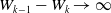 $W_{k-1}- W_k \rightarrow \infty$
as
$W_{k-1}- W_k \rightarrow \infty$
as
 $k \to \infty$
, hence
$k \to \infty$
, hence
 $ W_{k+1} - W_k\rightarrow - \infty$
. In the first case, we have that
$ W_{k+1} - W_k\rightarrow - \infty$
. In the first case, we have that
 $\alpha e^E e^{W_{k+1}- W_k } \sim e^{\sigma + k \Delta }$
as
$\alpha e^E e^{W_{k+1}- W_k } \sim e^{\sigma + k \Delta }$
as
 $k \to \infty$
, therefore
$k \to \infty$
, therefore
 $W_k \sim \frac {k^2}{2} \Delta$
as
$W_k \sim \frac {k^2}{2} \Delta$
as
 $k \to \infty$
. When instead we assume that
$k \to \infty$
. When instead we assume that
 $ W_{k-1} - W_k\rightarrow \infty$
, we deduce that
$ W_{k-1} - W_k\rightarrow \infty$
, we deduce that
 $\alpha e^E e^{W_{k-1}- W_k } \sim e^{\sigma + k \Delta }$
as
$\alpha e^E e^{W_{k-1}- W_k } \sim e^{\sigma + k \Delta }$
as
 $k \to \infty$
, hence
$k \to \infty$
, hence
 $W_k \sim - \frac { k^2}{2} \Delta$
as
$W_k \sim - \frac { k^2}{2} \Delta$
as
 $k \to \infty$
.
$k \to \infty$
.
Let
 $\psi _k^+ , \psi _k^-$
be two solutions to (8.4) such that
$\psi _k^+ , \psi _k^-$
be two solutions to (8.4) such that
 $\psi _k^+ \sim e^{\frac {k^2 }{2} \Delta }$
as
$\psi _k^+ \sim e^{\frac {k^2 }{2} \Delta }$
as
 $k \to \infty$
and
$k \to \infty$
and
 $\psi _k^- \sim e^{- \frac {k^2 }{2} \Delta }$
as
$\psi _k^- \sim e^{- \frac {k^2 }{2} \Delta }$
as
 $ k \to \infty$
. Let us define
$ k \to \infty$
. Let us define
 $\tilde {n}_k$
as
$\tilde {n}_k$
as
 \begin{equation*} \tilde {n}_k = n_k^{(p)} \tilde {n}_S + a \psi _k^+ + b \psi _k^-, \quad k \geq 0. \end{equation*}
Without loss of generality, we can assume that
 $\psi _0^+= \psi _1^+=1$
, so that
$\psi _0^+= \psi _1^+=1$
, so that
 $\psi ^+_k$
is unique, and we select
$\psi ^+_k$
is unique, and we select
 $a,b,\psi _0^- , \psi _1^+$
in such a way that
$a,b,\psi _0^- , \psi _1^+$
in such a way that
 \begin{equation*} a + b \psi _-^0 = \tilde {n}_0 = \frac { \tilde {n}_S + \alpha e^E \tilde {n}_1 }{ \alpha + e^\sigma } \text{ and } a +b\psi _-^1 =\hat {n}_1, \end{equation*}
where
 \begin{equation*} \frac { \tilde {n}_S }{1-e^{-E}} = e^{\sigma } \sum _{k=0}^{\infty } (n_k^{(p)} \tilde {n}_S + a \psi _k^+ ) e^{k \Delta } + b e^{\sigma } \sum _{k=0}^{\infty } \psi _k^- e^{k \Delta }. \end{equation*}
This implies that
 $n_k^{(p)}\sim - a \frac {\psi _k^+}{\tilde {n}_S}$
as
$n_k^{(p)}\sim - a \frac {\psi _k^+}{\tilde {n}_S}$
as
 $k \to \infty$
. More precisely,
$k \to \infty$
. More precisely,
 \begin{equation*} n_k^{(p)} \tilde {n}_S + a \psi _k^+ \sim e^{- \sigma - k (\Delta + E) } \text{ as } k \to \infty , \quad \psi _k^- \sim e^{- \frac {k^2}{2 } \Delta } \text{ as } k \to \infty \end{equation*}
Therefore, (8.3) holds.
8.2. Attachment rate depending on
$\Delta$

We consider a model in which the parameter
 $\Delta \gt 0$
affects the attachment rate. We show that this model can have strong discrimination properties under certain assumptions on the parameters.
$\Delta \gt 0$
affects the attachment rate. We show that this model can have strong discrimination properties under certain assumptions on the parameters.
We study the chemical reaction network generated by the following chemical reactions
 \begin{equation} S \overset {e^{- k (E+\Delta ) } }{\underset {e^{\sigma }} \rightleftarrows } C_k \overset {\alpha }{\underset {\alpha e^E }\rightleftarrows } C_{k+1} \overset {e^{\sigma }}{\underset {e^{- (k+1)(E+\Delta ) }} \rightleftarrows } S, \quad k \in \mathbb N. \end{equation}
The system of ODEs corresponding to this model is the following
 \begin{align} \frac {d n_S }{dt} &= - \frac {n_S}{1-e^{-E}} + e^{\sigma } \sum _{k=0}^{\infty } n_k e^{k (\Delta +E) } \nonumber\\[3pt] \frac {d n_0 }{dt} &= n_S - e^{\sigma } n_0 + \alpha e^E n_1 - \alpha n_0 \nonumber \\[3pt] \frac {d n_k }{dt} &= n_S e^{- k (E+\Delta ) } - ( e^{\sigma } + \alpha e^E + \alpha ) n_k + \alpha e^E n_{k+1} + \alpha n_{k-1} , \quad k \geq 1. \end{align}
We analyse the steady states
 $\tilde {n}=(\tilde {n}_S, \tilde {n}_k)_{k=0}^N$
of the system of ODEs (8.7). Using arguments that are analogues to the ones used in Section 4, we deduce that the solutions of the form
$\tilde {n}=(\tilde {n}_S, \tilde {n}_k)_{k=0}^N$
of the system of ODEs (8.7). Using arguments that are analogues to the ones used in Section 4, we deduce that the solutions of the form
 \begin{equation*} \tilde {n}_k = B \tilde {n}_S e^{- k (E+\Delta ) } + C g(\sigma )^k \end{equation*}
where
 \begin{equation*} g(\sigma ) = \frac {1}{2 } \left ( 1+ \frac {e^{\sigma -E}}{\alpha } + e^{-E} - \sqrt { \left (1+ \frac {e^{\sigma -E}}{\alpha } +e^{-E } \right )^2 - 4 e^{- E }} \right ) \lt 1 \end{equation*}
and where
 $B$
and
$B$
and
 $C$
are suitable constants. Moreover, the function
$C$
are suitable constants. Moreover, the function
 $f$
defined as
$f$
defined as
 \begin{equation*} f(\Delta )\,:\!=\, g(\sigma ) e^{ E+\Delta } \end{equation*}
is such that
 $f(0)\lt 1$
while
$f(0)\lt 1$
while
 $\lim _{\Delta \to \infty } f(\Delta ) \gt 1$
. As a consequence, there exists a
$\lim _{\Delta \to \infty } f(\Delta ) \gt 1$
. As a consequence, there exists a
 $\Delta _c$
such that if
$\Delta _c$
such that if
 $\Delta \lt \Delta _c$
, then the model does not have strong discrimination properties while if
$\Delta \lt \Delta _c$
, then the model does not have strong discrimination properties while if
 $\Delta \gt \Delta _c$
the model has strong discrimination properties, i.e. the steady state is given by
$\Delta \gt \Delta _c$
the model has strong discrimination properties, i.e. the steady state is given by
 $e^{- k \lambda (\sigma , E) }$
where
$e^{- k \lambda (\sigma , E) }$
where
 $\lambda (\sigma , E)$
depends on
$\lambda (\sigma , E)$
depends on
 $\sigma$
.
$\sigma$
.
8.3. Dephosphorylation rate depending on
$\Delta$

We assume now that
 $\Delta$
affects the dephosphorylation reaction. In this case, we can obtain strong discrimination only if
$\Delta$
affects the dephosphorylation reaction. In this case, we can obtain strong discrimination only if
 $\alpha$
, the phosphorylation rate, is sufficiently large. Consider the chemical reaction network generated by the following chemical reactions
$\alpha$
, the phosphorylation rate, is sufficiently large. Consider the chemical reaction network generated by the following chemical reactions
 \begin{equation} S \overset {e^{- k E} }{\underset {e^{\sigma }} \rightleftarrows } C_k \overset {\alpha }{\underset {\alpha e^{E-\Delta } }\rightleftarrows } C_{k+1} \overset {e^{\sigma }}{\underset {e^{- (k+1)E }} \rightleftarrows } S, \quad k \in \mathbb N. \end{equation}
We formulate the system of equations
 \begin{align} \frac {d n_S }{dt} &= - \frac {n_S}{1-e^{-E}} + e^{\sigma } \sum _{k=0}^{\infty } n_k e^{k E } \nonumber\\ \frac {d n_0 }{dt} &= n_S - e^{\sigma } n_0 + \alpha e^{E- \Delta } n_1 - \alpha n_0 \nonumber \\[3pt] \frac {d n_k }{dt} &= n_S e^{- k E } - \left ( e^{\sigma } + \alpha e^{E- \Delta } + \alpha \right ) n_k + \alpha e^{E- \Delta } n_{k+1} + \alpha n_{k-1} , \quad k \geq 1. \end{align}
The steady states
 $\tilde {n}=(\tilde {n}_S, \tilde {n}_k)_{k=0}^N$
of the system of ODEs (8.9) are given by
$\tilde {n}=(\tilde {n}_S, \tilde {n}_k)_{k=0}^N$
of the system of ODEs (8.9) are given by
 \begin{equation*} \tilde {n}_k = B \tilde {n}_S e^{- k E } + C g(\sigma )^k \end{equation*}
where
 $B, C$
are suitable constants depending on the parameters and where
$B, C$
are suitable constants depending on the parameters and where
 \begin{equation*} g(\sigma ) = \frac {1}{2 } \left [ 1+ e^{\Delta - E } + \frac {e^{\sigma + \Delta - E }}{ \alpha } - \sqrt { \left ( 1+ e^{\Delta - E } + \frac {e^{\sigma + \Delta - E }}{ \alpha } \right )^2 - 4 e^{\Delta - E }} \right ] \lt 1. \end{equation*}
In this case, we have that if
 $\frac {e^{\sigma - E }}{ \alpha (1- e^{- E } ) } \lt 1$
, then there exists a critical
$\frac {e^{\sigma - E }}{ \alpha (1- e^{- E } ) } \lt 1$
, then there exists a critical
 $\Delta _c$
 \begin{equation*} \Delta _c = \log \left ( \frac {1}{1-\frac {e^{\sigma - E }}{ \alpha (1- e^{- E } ) } } \right ) \gt 0 \end{equation*}
such that the asymptotic behaviour of
 $\tilde {n}_k$
as
$\tilde {n}_k$
as
 $k \to \infty$
depends on
$k \to \infty$
depends on
 $\sigma$
only when
$\sigma$
only when
 $\Delta \gt \Delta _c$
, i.e.
$\Delta \gt \Delta _c$
, i.e.
 $\tilde {n}_k \sim e^{ - k \lambda (\sigma , E) }$
as
$\tilde {n}_k \sim e^{ - k \lambda (\sigma , E) }$
as
 $k \to \infty$
where
$k \to \infty$
where
 $\lambda (\sigma , E)$
depends on
$\lambda (\sigma , E)$
depends on
 $\sigma$
only when
$\sigma$
only when
 $\Delta \gt \Delta _c$
.
$\Delta \gt \Delta _c$
.
8.4.
$\Delta \to \infty$
and
$\alpha e^{\Delta } \approx 1$


In this section, we derive the one-directional model that we analysed in [Reference Franco and Velázquez11] as a limit case of the model studied in this paper.
We consider the model with infinite states, i.e. we assume that the model is described by (5.1). We now study the steady states that satisfy (4.3)–(4.4). As explained in Section 5, the behaviour of the steady states is expected to be the following one
 \begin{equation*} \tilde {n}_k \sim e^{- k E } A(0) \overline n_S \left [ 1 + B \varphi (\sigma )^k \right ], \text{ as } k \to \infty \end{equation*}
where
 $B$
is given by (4.9) and where
$B$
is given by (4.9) and where
 $\varphi (\sigma )$
is given by (4.7). We assume that
$\varphi (\sigma )$
is given by (4.7). We assume that
 $\alpha e^\Delta =\gamma \approx 1$
, then
$\alpha e^\Delta =\gamma \approx 1$
, then
 \begin{align*} \varphi (\sigma )&= \frac {1}{2 \alpha } \left ( e^\sigma + \alpha \left(e^E+ e^\Delta \right) \right ) \left ( 1 - \sqrt { 1- \frac {4 \alpha ^2 e^{\Delta + E }}{(e^\sigma + \alpha (e^E+ e^\Delta ) )^2 } } \right ) \\ & \sim \frac { \alpha e^{\Delta + E }}{e^\sigma + \alpha (e^E+ e^\Delta ) } \sim e^E \frac {1}{1 + \frac {e^\sigma }{\gamma } }, \text{ as } \Delta \to \infty . \end{align*}
Since we have that
 \begin{equation*} \tilde {n}_k \sim e^{- k E } A(0) \overline n_S \left [ 1 + B \varphi (\sigma )^k \right ], \text{ as } k \to \infty \end{equation*}
we deduce that
 $\tilde {n}_k \sim e^{-\lambda (\sigma , E) k }$
where
$\tilde {n}_k \sim e^{-\lambda (\sigma , E) k }$
where
 $\lambda (\sigma , E) = E$
if
$\lambda (\sigma , E) = E$
if
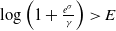 $\log \left (1+ \frac {e^\sigma }{\gamma } \right )\gt E$
while
$\log \left (1+ \frac {e^\sigma }{\gamma } \right )\gt E$
while
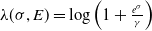 $ \lambda (\sigma , E) = \log \left (1+ \frac {e^\sigma }{\gamma } \right )$
when
$ \lambda (\sigma , E) = \log \left (1+ \frac {e^\sigma }{\gamma } \right )$
when
 $\log \left (1+ \frac {e^\sigma }{\gamma } \right ) \lt E$
. In the second case, we have strong discrimination properties because
$\log \left (1+ \frac {e^\sigma }{\gamma } \right ) \lt E$
. In the second case, we have strong discrimination properties because
 $\lambda (\sigma , E)$
depends on
$\lambda (\sigma , E)$
depends on
 $\sigma$
.
$\sigma$
.
In order to understand the condition for discrimination
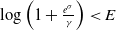 $\log \left (1+ \frac {e^\sigma }{\gamma } \right ) \lt E$
, recall that
$\log \left (1+ \frac {e^\sigma }{\gamma } \right ) \lt E$
, recall that
 \begin{equation*} \Delta _c = \log \left (1+ \frac {e^\sigma }{ \alpha (e^E-1) } \right ) . \end{equation*}
Assume now that
 $\Delta \to \infty$
and that
$\Delta \to \infty$
and that
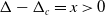 $\Delta - \Delta _c = x \gt 0$
. Under this assumption, we expect the limiting model to have strong discrimination properties. This assumption implies that the parameters satisfy the assumption
$\Delta - \Delta _c = x \gt 0$
. Under this assumption, we expect the limiting model to have strong discrimination properties. This assumption implies that the parameters satisfy the assumption
 $\log \left (1+ \frac {e^\sigma }{\gamma } \right ) \lt E$
, indeed
$\log \left (1+ \frac {e^\sigma }{\gamma } \right ) \lt E$
, indeed
 \begin{equation*} 1 \lt e^{x } = e^{ - \Delta } + \frac {e^{\sigma -\Delta } }{ \alpha (e^E-1) } \sim \frac {e^{\sigma } }{ \gamma (e^E-1) } \text{ as } \Delta \to \infty . \end{equation*}
In the model that we consider in [Reference Franco and Velázquez11], we have that
 $E=\infty$
. Indeed, in that paper, we assume that when the ligands attach to the receptors, then they form a complex that has always state
$E=\infty$
. Indeed, in that paper, we assume that when the ligands attach to the receptors, then they form a complex that has always state
 $0.$
In that case is always true that
$0.$
In that case is always true that
 $ \log \left ( 1+ \frac {e^\sigma }{\gamma } \right ) \lt E= \infty$
, hence we always have discrimination.
$ \log \left ( 1+ \frac {e^\sigma }{\gamma } \right ) \lt E= \infty$
, hence we always have discrimination.
9. Conclusions and open problems
In this paper, we prove that a minimal amount of lack of detailed balance is necessary in order to have strong discrimination properties. In other words, we prove that the kinetic proofreading systems must be out of equilibrium systems. This absence of equilibrium can be measured in terms of the frozen concentrations of some substances, like ATP or ADP, that must be sufficiently far from equilibrium.
Given that the lack of detailed balance is a property on the chemical rates of the reactions that belong to the cycles, one could think that similar amounts of lack of detailed balance would result in a similar behaviour of the network. We prove that this is not the case. We give examples of models that have identical amount of lack of detailed balance and that do not have the same discrimination properties.
We also have shown that in some parameter regimes, the chemical network studied in this paper can be approximated by means of PDEs for which the mathematical analysis of the discrimination properties is more amenable.
It could be interesting to study the behaviour of the network when the lack of detailed balance
 $\Delta _k$
in the phosphorylation reaction
$\Delta _k$
in the phosphorylation reaction
 $C_k \rightarrow C_{k+1}$
depends on
$C_k \rightarrow C_{k+1}$
depends on
 $k$
. It would be relevant to understand if also in this case a critical amount of detailed balance is needed in order to have strong discrimination.
$k$
. It would be relevant to understand if also in this case a critical amount of detailed balance is needed in order to have strong discrimination.
We could also consider more complex models in which the phosphorylation reaction is modelled in more detail. In particular, we can assume that phosphorylation is a chain of reactions that involves
 $ATP$
,
$ATP$
,
 $ADP$
and phosphate groups, but also other substances that are out of equilibrium, for instance, some enzymes. It would be relevant to understand if including these substances in the system, hence changing the topology of the network, can improve the discrimination properties of the chemical network.
$ADP$
and phosphate groups, but also other substances that are out of equilibrium, for instance, some enzymes. It would be relevant to understand if including these substances in the system, hence changing the topology of the network, can improve the discrimination properties of the chemical network.
In this paper, we analyse in detail the discrimination property of the kinetic proofreading mechanism and its relation with detailed balance. Understanding if a biological function can be achieved by passive systems (with detailed balance) or if it requires active processes is a relevant question for several biological systems. For instance, in [Reference Franco and Velázquez12], we analyse whether the property of adaptation, which takes place in many relevant signalling systems, can be achieved or not by equilibrium chemical reaction networks.
Funding statement
The authors gratefully acknowledge the support of the grant CRC 1720 ‘Analysis of Criticality: from Complex Phenomena to Models and Estimates’ (Project-ID 539309657) of the University of Bonn funded through the Deutsche Forschungs- gemeinschaft (DFG, German Research Foundation) and Germany’s Excellence Strategy-EXC-2047/2–390685813. The funders had no role in study design, analysis, decision to publish or preparation of the manuscript.
Competing interests
No competing interest to declare.
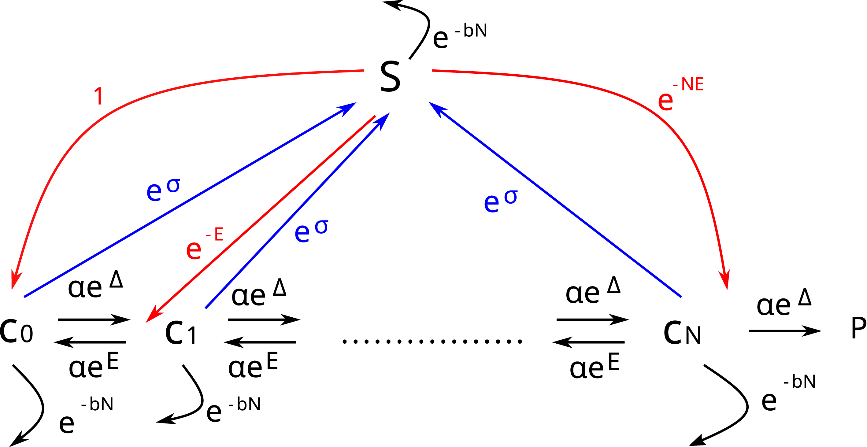
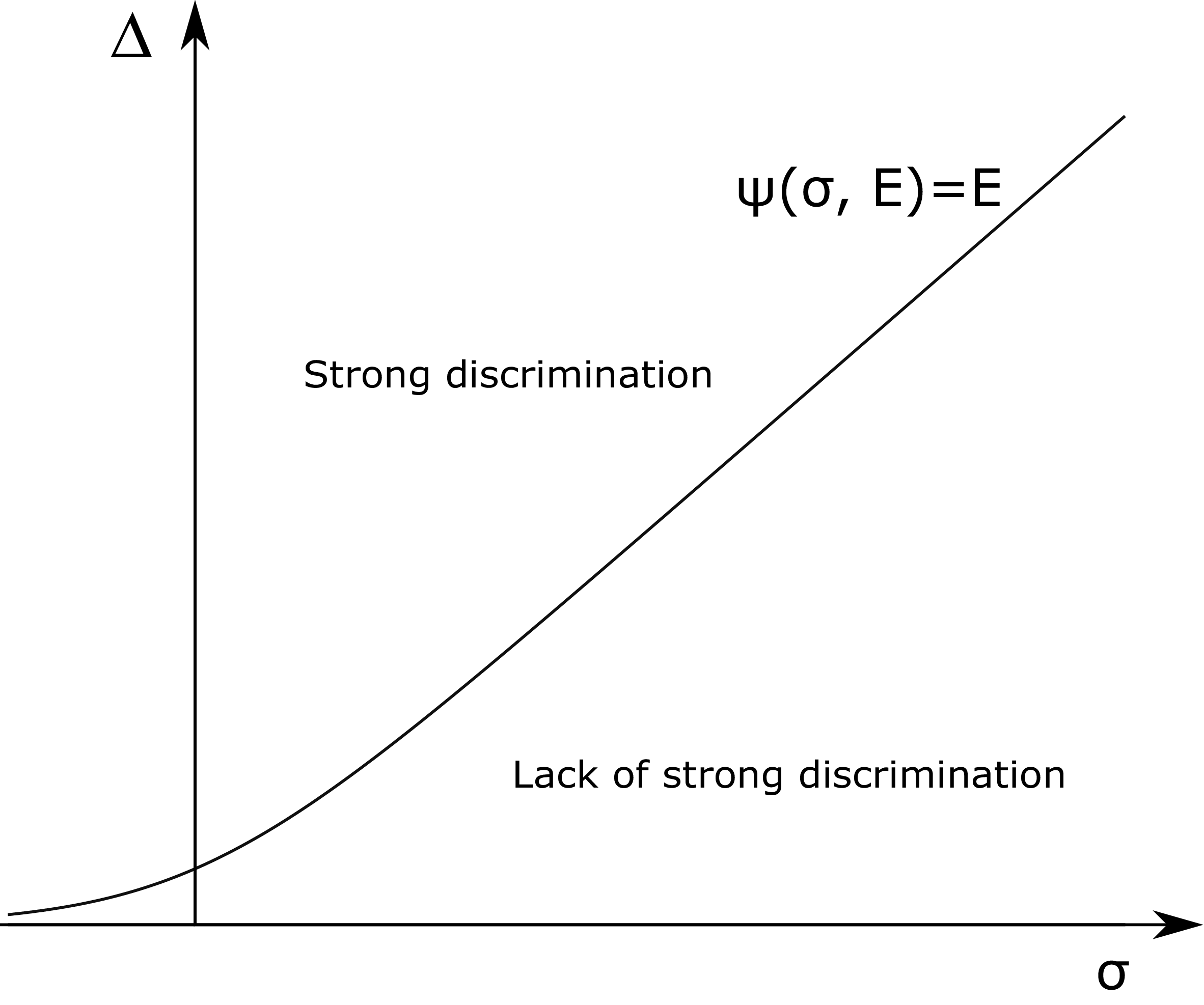


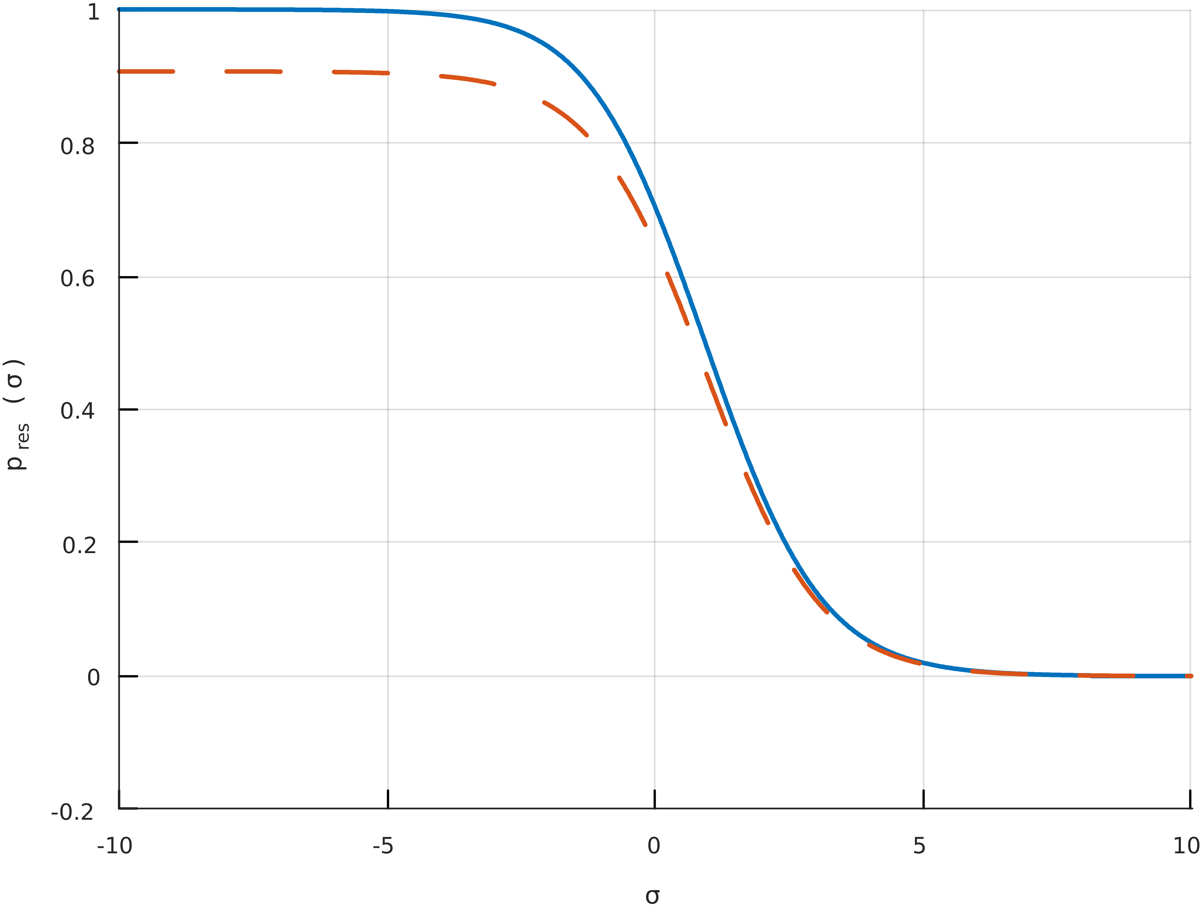


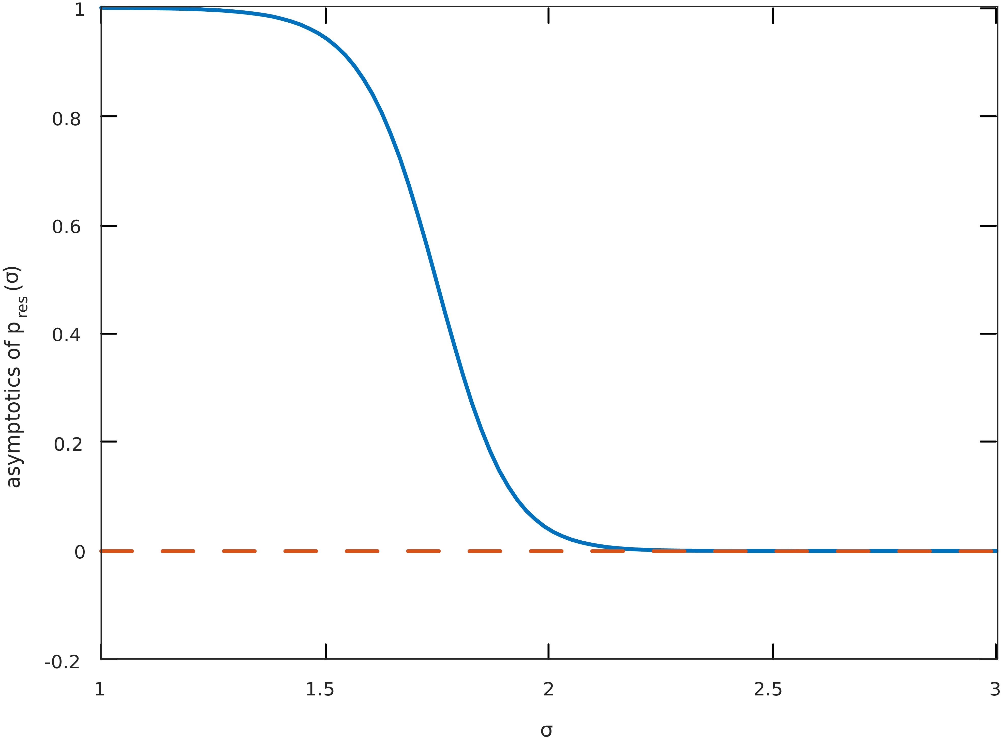


 Open access