




1 Introduction and motivation
Modern cyber-physical systems (CPSs) are rapidly growing in size and complexity, making rigorous verification increasingly costly. Using high-level, near-natural specifications with early verification can help mitigate this, but such requirements must first be translated into an appropriate formal language for verification.
Event Calculus (EC) has recently been advocated as a suitable formalism for this purpose, for example by Varanasi et al. (Reference Varanasi, Arias, Salazar, Li, Basu and Gupta2022), Murugesan et al. (Reference Murugesan, Wong, Arias, Stroud, Varadarajan, Salazar, Gupta, Bloomfield and Rushby2024), and Vašíček et al. (Reference Vašíček, Arias, Fiedor, Gupta, Hall, Křena, Larson, Varanasi and Vojnar2024). EC is a logical formalism for reasoning about events and change and is well suited for the given purpose due to its small semantic gap with semi-formal natural language requirements. In particular, Vašíček et al. (Reference Vašíček, Arias, Fiedor, Gupta, Hall, Křena, Larson, Varanasi and Vojnar2024) illustrates this by analyzing a real-life safety-critical system with an open-source high-level specification, which led to the discovery of a number of inconsistencies and a safety violation in the specification.
However, while EC allows natural modeling of CPS specifications, the resulting models typically use large or even dense value domains and describe continuous behavior. Analyzing such models is a significant challenge for current state-of-the-art general-purpose reasoning tools for EC, which are based on Answer Set Programming (ASP). Grounding-based ASP solvers, for example clingo by Gebser et al. (Reference Gebser, Kaminski, Kaufmann and Schaub2019), require discretization of dense domains, which can lead to inaccurate representation of the system. This can be avoided on a case-by-case basis by finding the right discretization (e.g., increasing the precision from seconds to milliseconds), but then the value and time domains can easily become large, making the solvers run out of resources due to an explosion in the size of the grounded program. The grounding-free ASP solver s(CASP) by Arias et al. (Reference Arias, Carro, Salazar, Marple and Gupta2018) does not discretize but faces non-termination issues.
To address these issues, we introduce Hybrid EC, an extension of the Discrete EC (DEC) axiomatization of Mueller (Reference Mueller2014). Hybrid EC introduces the so-called functional fluents to represent various system properties. The values of such fluents are represented using constraints. Moreover, Hybrid EC replaces the integer-time semantics of DEC with abstract step indices representing the sequence of system evolution. These steps are subsequently mapped to time through constraints.
We then utilize clingcon and clingo-lpx, Hybrid ASP solvers supporting linear constraints over integers and rationals, to implement the proposed Hybrid EC through the HEC axioms. Execution under Hybrid ASP avoids the grounding-size explosion with respect to time and value domains. More importantly, the HEC implementation enables accurate modeling of and reasoning about continuous change since clingo-lpx supports the representation of dense domains using rationals. This allows reasoning without discretization and eliminates inaccuracies due to discretized representations.
We have implemented and analyzed several examples from the literature to demonstrate the modeling capabilities and performance of our approach using clingcon and clingo-lpx. We compare the results with those obtained from the plain ASP solver clingo. Our hybrid approach scales independently of the size of the time and value domains, while the plain ASP approach does not. Furthermore, the use of rationals enables accurate modeling of continuous change, which was not possible previously, without affecting scalability compared to reasoning over integers.
2 Background
This section provides a brief overview of EC, a formalism for reasoning about events and change, initially proposed by Kowalski and Sergot (Reference Kowalski and Sergot1986) and Shanahan (Reference Shanahan1997), and Hybrid ASP, an extension of ASP that incorporates linear constraints.
2.1 Event Calculus
Several versions of EC have been proposed, see survey by Mueller (Reference Mueller2008), among which the most relevant are the EC and the DEC by Mueller (Reference Mueller2004) formulated for non-monotonic reasoning using first order logic and circumscription. EC was later reformulated by Lee and Palla (Reference Lee and Palla2012) in the theory of stable models and translated into ASP. Throughout the paper, we use the ASP encoding of DEC in code listings and as the base of our hybrid formulation of EC.
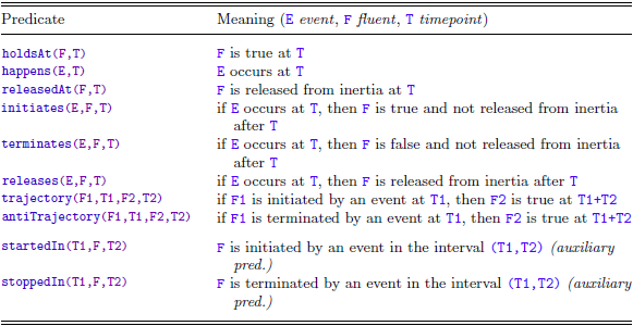
There are three basic concepts in EC: events representing actions that may occur in the world; fluents modeling time-varying properties of the world; and timepoints representing instants of time. Events may happen at a timepoint. Properties represented by fluents change discretely via events and stay constant between occurrences of the events due to inertia. When released from inertia, they change continuously via (anti-)trajectories or are non-deterministic. Predicates used in EC and DEC are listed in Table 1. A comprehensive introduction to EC can be found in Mueller (Reference Mueller2014).
Predicates used in EC and DEC. Based on Table 17.4 from Reference MuellerMueller (2008)

EC specifications of problem instances consist of a universal theory, a domain description, and a narrative. The theory is a conjunction of EC axioms, the domain description consists of the causal laws of the domain, and the narrative provides observations of event occurrences and about fluents. A basic example encoded using DEC follows:
Example 1 (Counter

 Footnote
1
)
Footnote
1
)
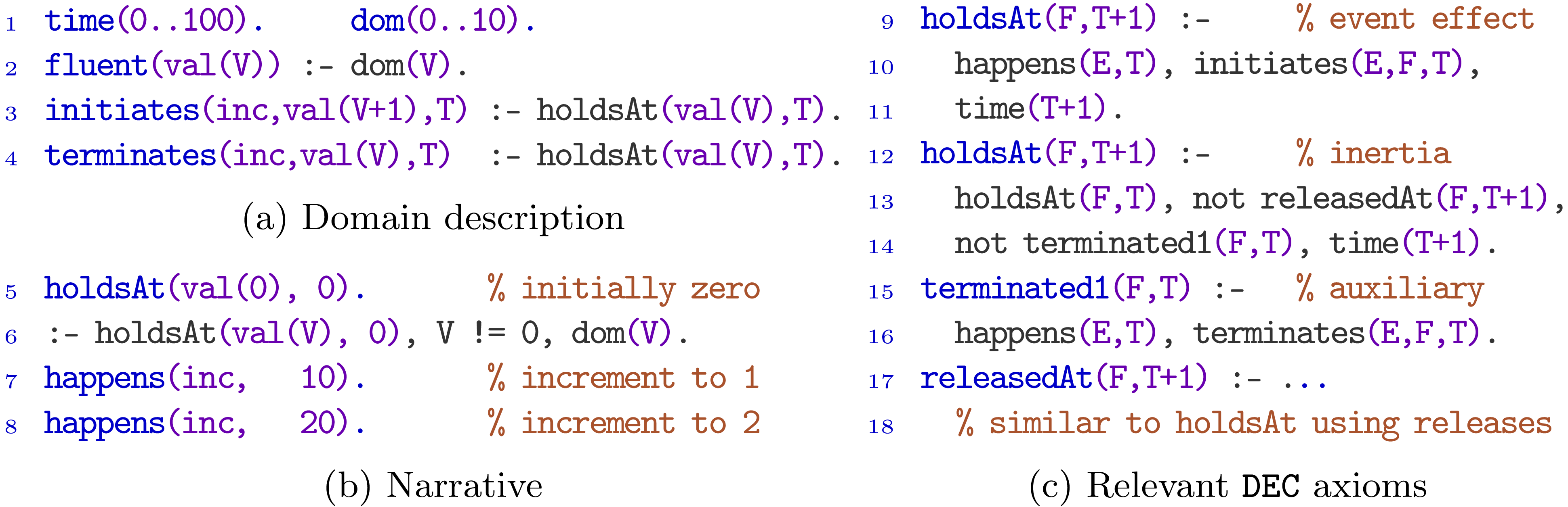
Consider the example from Mueller (Reference Mueller2008) that models a counter that can be incremented or reset. Figure 1(a) models a fragment (omitting the reset) of the rules of the domain, defining the fluent $\color{blue}{\texttt{val(V)}}$
, the
$\color{blue}{\texttt{val(V)}}$
, the $\color{blue}{\texttt{inc}}$
event, and its conditional effects on the fluent. Then, Figure 1(b) models the narrative of initial observations and event occurrences. For this narrative,
$\color{blue}{\texttt{inc}}$
event, and its conditional effects on the fluent. Then, Figure 1(b) models the narrative of initial observations and event occurrences. For this narrative, $\color{blue}{\texttt{val(1)}}$
would hold at all timepoints in the interval
$\color{blue}{\texttt{val(1)}}$
would hold at all timepoints in the interval $\color{blue}{\texttt{(10,20]}}$
. Finally, Figure 1(c) models the relevant DEC axioms defining when a fluent holds.
$\color{blue}{\texttt{(10,20]}}$
. Finally, Figure 1(c) models the relevant DEC axioms defining when a fluent holds.
DEC encoding of the counter example.

2.2 Hybrid ASP
We rely on a basic acquaintance with ASP. The syntax of our logic programs follows the one of clingo by Gebser et al. (Reference Gebser, Kaminski, Kaufmann, Lindauer, Ostrowski, Romero, Schaub and Thiele2015b); its semantics are detailed by Gebser et al. (Reference Gebser, Harrison, Kaminski, Lifschitz and Schaub2015a). The Hybrid ASP systems clingcon and clingo-lpxFootnote 2 extend the input language of clingo by theory atoms representing linear constraints that have the form

where $k\ge 0$
, the
$k\ge 0$
, the $\alpha _i$
’s and
$\alpha _i$
’s and $\beta$
are numeral terms, the
$\beta$
are numeral terms, the $t_i$
’s are symbolic terms, and
$t_i$
’s are symbolic terms, and $\circ \in \{\lt , \lt =, =, \gt =, \gt , ! \!= \}$
. Such a theory atom represents the linear constraint
$\circ \in \{\lt , \lt =, =, \gt =, \gt , ! \!= \}$
. Such a theory atom represents the linear constraint
 \begin{equation*} \alpha _1 \cdot t_1 + \ldots + \alpha _k \cdot t_k \circ \beta \end{equation*}
where $t_1$
, …,
$t_1$
, …, $t_k$
serve as variables, and the
$t_k$
serve as variables, and the $\alpha _i$
’s and
$\alpha _i$
’s and $\beta$
stand for integer constants. For convenience,
$\beta$
stand for integer constants. For convenience, $\alpha _i$
*
$\alpha _i$
* $t_i$
may be written as
$t_i$
may be written as $\alpha _i$
or
$\alpha _i$
or $t_i$
, and
$t_i$
, and $\beta$
may also be of the form
$\beta$
may also be of the form $\alpha$
*
$\alpha$
* $t$
,
$t$
, $\alpha$
or
$\alpha$
or $t$
.
$t$
.
In clingcon by Banbara et al. (Reference Banbara, Kaufmann, Ostrowski and Schaub2017), stable models are extended by an assignment from symbolic terms to integers. Theory atoms are evaluated with respect to that assignment, and symbolic terms are left open: they are not required to be founded and can therefore take any integer value without being justified by a rule. The semantics of clingo-lpx are the same as for clingcon, except that the assignment maps symbolic terms to rationals.Footnote 3
These hybrid systems do not ground symbolic terms over their possible values but instead rely on dedicated algorithms for linear constraints. This reduces grounding size and often improves solving performance. Additionally, clingo-lpx extends the expressiveness of clingo by supporting reasoning about rational numbers.
Example 2 (Falling Object) Consider the example by Mueller (Reference Mueller2014) of an object falling at constant speed. The following program represents the height of the object at two time steps (without EC):

The term $\color{blue}{\texttt{time(1)}}$
denotes the time passed at step
$\color{blue}{\texttt{time(1)}}$
denotes the time passed at step $\color{blue}{\texttt{1}}$
, while
$\color{blue}{\texttt{1}}$
, while $\color{blue}{\texttt{(height,0)}}$
and
$\color{blue}{\texttt{(height,0)}}$
and $\color{blue}{\texttt{(height,1)}}$
denote the height of the object at steps
$\color{blue}{\texttt{(height,1)}}$
denote the height of the object at steps $\color{blue}{\texttt{0}}$
and
$\color{blue}{\texttt{0}}$
and $\color{blue}{\texttt{1}}$
, respectively. The first rule requires the
$\color{blue}{\texttt{1}}$
, respectively. The first rule requires the $\color{blue}{\texttt{time}}$
at step
$\color{blue}{\texttt{time}}$
at step $\color{blue}{\texttt{1}}$
to be greater than
$\color{blue}{\texttt{1}}$
to be greater than $\color{blue}{\texttt{0}}$
. The
$\color{blue}{\texttt{0}}$
. The $\color{blue}{\texttt{height}}$
at step
$\color{blue}{\texttt{height}}$
at step $\color{blue}{\texttt{0}}$
is left open. If it is above
$\color{blue}{\texttt{0}}$
is left open. If it is above $\color{blue}{\texttt{0}}$
, then the second rule makes
$\color{blue}{\texttt{0}}$
, then the second rule makes $\color{blue}{\texttt{falling}}$
true, and consequently the third rule sets the
$\color{blue}{\texttt{falling}}$
true, and consequently the third rule sets the $\color{blue}{\texttt{height}}$
at
$\color{blue}{\texttt{height}}$
at $\color{blue}{\texttt{1}}$
to be the initial
$\color{blue}{\texttt{1}}$
to be the initial $\color{blue}{\texttt{height}}$
minus
$\color{blue}{\texttt{height}}$
minus $\color{blue}{\texttt{2}}$
times the time passed at step
$\color{blue}{\texttt{2}}$
times the time passed at step $\color{blue}{\texttt{1}}$
. Otherwise, the fourth rule makes the
$\color{blue}{\texttt{1}}$
. Otherwise, the fourth rule makes the $\color{blue}{\texttt{height}}$
at
$\color{blue}{\texttt{height}}$
at $\color{blue}{\texttt{1}}$
persist from step
$\color{blue}{\texttt{1}}$
persist from step $\color{blue}{\texttt{0}}$
. This program has one stable model for every value of
$\color{blue}{\texttt{0}}$
. This program has one stable model for every value of $\color{blue}{\texttt{(height,0)}}$
and every value of
$\color{blue}{\texttt{(height,0)}}$
and every value of $\color{blue}{\texttt{time(1)}}$
greater than
$\color{blue}{\texttt{time(1)}}$
greater than $\color{blue}{\texttt{0}}$
. If
$\color{blue}{\texttt{0}}$
. If $\color{blue}{\texttt{(height,0)}}$
is above
$\color{blue}{\texttt{(height,0)}}$
is above $\color{blue}{\texttt{0}}$
, then
$\color{blue}{\texttt{0}}$
, then $\color{blue}{\texttt{falling}}$
belongs to the model and the value of
$\color{blue}{\texttt{falling}}$
belongs to the model and the value of $\color{blue}{\texttt{(height,1)}}$
is given by the expression
$\color{blue}{\texttt{(height,1)}}$
is given by the expression $\color{blue}{\texttt{(height,0)-2*time(1)}}$
. Otherwise,
$\color{blue}{\texttt{(height,0)-2*time(1)}}$
. Otherwise, $\color{blue}{\texttt{falling}}$
is not in the model and
$\color{blue}{\texttt{falling}}$
is not in the model and $\color{blue}{\texttt{(height,1)}}$
has the same value as
$\color{blue}{\texttt{(height,1)}}$
has the same value as $\color{blue}{\texttt{(height,0)}}$
.
$\color{blue}{\texttt{(height,0)}}$
.
3 Related work
Automated reasoning techniques for the EC have evolved over time. An early approach is the Prolog-based EC planner by Shanahan (Reference Shanahan2000). This was later followed by the SAT-based DEC reasoner by Mueller (Reference Mueller2014). More recently, Lee and Palla (Reference Lee and Palla2012) reformulated the EC in terms of ASP and provided the automated transformation tools EC2ASP and F2LP. This enabled the use of state-of-the-art ASP solvers, such as clingo by Gebser et al. (Reference Gebser, Kaminski, Kaufmann and Schaub2019), which offer superior performance and expressiveness compared to the earlier approaches. All these approaches considered only discrete time and discrete values of fluents. This restriction is inherent to SAT- and ASP-based methods, as the ground phase requires finite domains and this precludes the representation of infinite/dense domains. Moreover, grounding can lead to the well-known grounding explosion as the size of the domain increases.
Alternative approaches for reasoning about EC, for example by Arias et al. (Reference Arias, Carro, Chen and Gupta2022) and Vašíček et al. (Reference Vašíček, Arias, Fiedor, Gupta, Hall, Křena, Larson, Varanasi and Vojnar2024, Reference Vašíček, Arias, Fiedor, Gupta, Hall, Křena, Larson and Vojnar2025), use s(CASP), a grounding-free, query-driven ASP solver by Arias et al. (Reference Arias, Carro, Salazar, Marple and Gupta2018) which supports linear constraints over rationals. To the best of our knowledge, these are the only ones for fully-automated, general-purpose, logical reasoning about EC that reasons considering continuous change while avoiding the grounding explosion and offering multiple reasoning modes, including abduction. However, as an academic prototype, s(CASP) lacks the optimized performance of clingo and, further, can suffer from non-termination problems due to its query-driven, Prolog-style execution.
There are other systems that extend ASP with linear constraints, for example those based on translation-based approaches, such as EZSMT or ASPMT2SMT, and constraint propagation approaches, such as DLVHEX[CP] or EZCSP, which each have their own advantages and disadvantages—for a comprehensive survey see the work by Lierler (Reference Lierler2023).
Finally, there exists a wide range of specialized applications of EC, which often use their own specialized tool for the reasoning. Such tools typically offer much better performance but only for a particular class of problems or for specific reasoning tasks. For example, RTEC by Artikis et al. (Reference Artikis, Sergot and Paliouras2015) supports reasoning in real-time and is specialized in monitoring streams of events to detect composite events.
4 Hybrid EC
The main goal of our work is to reason about EC with continuous changes and, thus, with dense value domains of fluents and time. Traditional ASP solvers, such as clingo, fully ground the program. On the other hand, Hybrid ASP allows one to keep only part of the model grounded, while other parts can be represented by constraints, in such a way that they are not grounded, and, thus, we can use these constraints to represent dense and/or infinite domains. In this section, we present Hybrid EC, an extended axiomatization of DEC, a formulation introduced by Mueller (Reference Mueller2014) that has been proven to be equivalent to the EC formulation when restricted to integers. The core aspect of DEC is that it operates timepoint by timepoint instead of over spans of timepoints, that is always referencing two consecutive timepoints $\color{blue}{\texttt{T}}$
and
$\color{blue}{\texttt{T}}$
and $\color{blue}{\texttt{T+1}}$
. Hybrid EC further introduces two core ideas:
$\color{blue}{\texttt{T+1}}$
. Hybrid EC further introduces two core ideas:
-
1. The definition of functional fluents that can hold dense values since these values (and the relations among them) can be represented by constraints and, thus, can be grounding-free (Section 4.1).
-
2. A hybrid representation of time where significant timepoints are mapped to discrete steps of the system and only those are grounded, while the actual time is handled by the constraint solver and is, thus, grounding-free and can be dense (Section 4.2).
In addition, we present HEC, an implementation of Hybrid EC in Hybrid ASP, that builds on the ASP-based encoding of DEC proposed by Lee and Palla (Reference Lee and Palla2012) and utilizes the two above-mentioned ideas. The implementation incrementally executes a Hybrid ASP solver, either clingcon or clingo-lpx (Section 5), gradually increasing the number of steps in the hybrid representation of time until a model is found (Section 4.6). It utilizes the Hybrid ASP encoding of our HEC axioms (Section 4.3) along with additional rules for handling observations defined in a narrative (Section 4.4) and events triggered via continuous change or time (Section 4.5). A problem instance then needs to provide a general encoding of the domain description and a particular narrative.
4.1 Functional fluents
Fluents in EC represent time-varying properties of the world: for example $\color{blue}{\texttt{falling(apple)}}$
represents that an apple is falling, and
$\color{blue}{\texttt{falling(apple)}}$
represents that an apple is falling, and $\color{blue}{\texttt{height(apple,Value)}}$
represents the height of the apple within a given range of numerical values. Standard EC supports only relational fluents, that is, fluents are either true or false at any given timepoint, which is represented as
$\color{blue}{\texttt{height(apple,Value)}}$
represents the height of the apple within a given range of numerical values. Standard EC supports only relational fluents, that is, fluents are either true or false at any given timepoint, which is represented as $\color{blue}{\texttt{holdsAt(Fluent,Time)}}$
or its negation. In DEC, fluents are ground atoms, for example
$\color{blue}{\texttt{holdsAt(Fluent,Time)}}$
or its negation. In DEC, fluents are ground atoms, for example $\color{blue}{{\texttt{height(apple,1)}}, \ldots, {\texttt{height(apple,10)}}}$
Footnote
4
that, in principle, can hold at the same time. The situation calculus by Lee and Palla (Reference Lee and Palla2012) supports functional fluents, which can take different values, for example
$\color{blue}{{\texttt{height(apple,1)}}, \ldots, {\texttt{height(apple,10)}}}$
Footnote
4
that, in principle, can hold at the same time. The situation calculus by Lee and Palla (Reference Lee and Palla2012) supports functional fluents, which can take different values, for example $\color{blue}{\texttt{height(apple)=Value}}$
. According to Mueller (Reference Mueller2014), functional fluents can be represented by relational fluents in EC, for example,
$\color{blue}{\texttt{height(apple)=Value}}$
. According to Mueller (Reference Mueller2014), functional fluents can be represented by relational fluents in EC, for example, $\color{blue}{\texttt{f(X)=Y}}$
can be encoded as
$\color{blue}{\texttt{f(X)=Y}}$
can be encoded as $\color{blue}{\texttt{f(X,Y)}}$
, provided that for any
$\color{blue}{\texttt{f(X,Y)}}$
, provided that for any $\color{blue}{\texttt{X}}$
and
$\color{blue}{\texttt{X}}$
and $\color{blue}{\texttt{T}}$
there is exactly one
$\color{blue}{\texttt{T}}$
there is exactly one $\color{blue}{\texttt{Y}}$
such that
$\color{blue}{\texttt{Y}}$
such that $\color{blue}{\texttt{holdsAt(f(X,Y),T)}}$
.
$\color{blue}{\texttt{holdsAt(f(X,Y),T)}}$
.
We introduce functional fluents in EC using the language of Hybrid ASP. The value of a functional fluent $\color{blue}{\texttt{F}}$
at a step
$\color{blue}{\texttt{F}}$
at a step $\color{blue}{\texttt{S}}$
is given by the symbolic term
$\color{blue}{\texttt{S}}$
is given by the symbolic term $\color{blue}{\texttt{(F,S)}}$
. A value
$\color{blue}{\texttt{(F,S)}}$
. A value $\color{blue}{\texttt{Val}}$
can be assigned to this term using the theory atom
$\color{blue}{\texttt{Val}}$
can be assigned to this term using the theory atom $\color{blue}{\texttt{&sum(F,S)=Val}}$
. Recall that in clingcon and clingo-lpx, the values of symbolic terms are left open. This corresponds closely to the relational representation of DEC by Lee and Palla (Reference Lee and Palla2012), where fluent values are left open using choice rules of the form
$\color{blue}{\texttt{&sum(F,S)=Val}}$
. Recall that in clingcon and clingo-lpx, the values of symbolic terms are left open. This corresponds closely to the relational representation of DEC by Lee and Palla (Reference Lee and Palla2012), where fluent values are left open using choice rules of the form $\color{blue}{\texttt{\{holdsAt(F,T)\}}}$
.
$\color{blue}{\texttt{\{holdsAt(F,T)\}}}$
.
4.2 Hybrid representation of time
DEC uses integer time steps, and all predicates are grounded to all timepoints. However, all changes in EC are caused by event occurrences, and fluents either maintain a constant value or their value changes via a trajectory between occurrences. Therefore, one can focus the reasoning only on the significant timepoints, that is, those with event occurrences, seeing them as states. We propose to treat DEC time steps as abstract steps of the system instead of integer increments of time. Each step corresponds to the occurrence of an event, representing the state of the system at the time of occurrence and the state transition initiated by it. The number of steps must be equal to the number of event occurrences at distinct timepoints plus one step for an implicit final state that allows us to observe the effects of the last event. Each step then has a timepoint associated with it via constraints. This means that a variable amount of time can pass between each pair of subsequent steps and that the grounding size is determined by the number of steps instead of the size of the time domain. A limitation of this approach is that, currently, we must specify the number of steps to be used when executing the reasoning. For now, assume that we guess the right number of steps, we explain an incremental execution approach in Section 4.6.
Figure 2 shows the encoding of this hybrid representation, where the time at step $\color{blue}{\texttt{S}}$
is denoted by the symbolic term
$\color{blue}{\texttt{S}}$
is denoted by the symbolic term $\color{blue}{\texttt{(time,S)}}$
. Lines 1–3 define the time of the first and last steps and ensure that the time associated with consecutive steps is strictly increasing. Within this representation, an atom
$\color{blue}{\texttt{(time,S)}}$
. Lines 1–3 define the time of the first and last steps and ensure that the time associated with consecutive steps is strictly increasing. Within this representation, an atom $\color{blue}{\texttt{holdsAt(F,S)}}$
expresses that a relational fluent
$\color{blue}{\texttt{holdsAt(F,S)}}$
expresses that a relational fluent $\color{blue}{\texttt{F}}$
holds at step
$\color{blue}{\texttt{F}}$
holds at step $\color{blue}{\texttt{S}}$
. For
$\color{blue}{\texttt{S}}$
. For $\color{blue}{\texttt{S=0}}$
, this means that
$\color{blue}{\texttt{S=0}}$
, this means that $\color{blue}{\texttt{F}}$
holds in the time interval
$\color{blue}{\texttt{F}}$
holds in the time interval $\color{blue}{\texttt{[0,(time,0)]}}$
, while for
$\color{blue}{\texttt{[0,(time,0)]}}$
, while for
 ,
, $\color{blue}{\texttt{F}}$
holds in
$\color{blue}{\texttt{F}}$
holds in $\color{blue}{\texttt{((time,S-1),(time,S)]}}$
. Note that
$\color{blue}{\texttt{((time,S-1),(time,S)]}}$
. Note that $\color{blue}{\texttt{(time,0)}}$
may be greater than zero. Fluents that undergo continuous change have a specific value at each step
$\color{blue}{\texttt{(time,0)}}$
may be greater than zero. Fluents that undergo continuous change have a specific value at each step $\color{blue}{\texttt{S}}$
, but their value changes between steps according to the corresponding trajectory.
$\color{blue}{\texttt{S}}$
, but their value changes between steps according to the corresponding trajectory.
Mapping of (dense) time values to discrete steps.

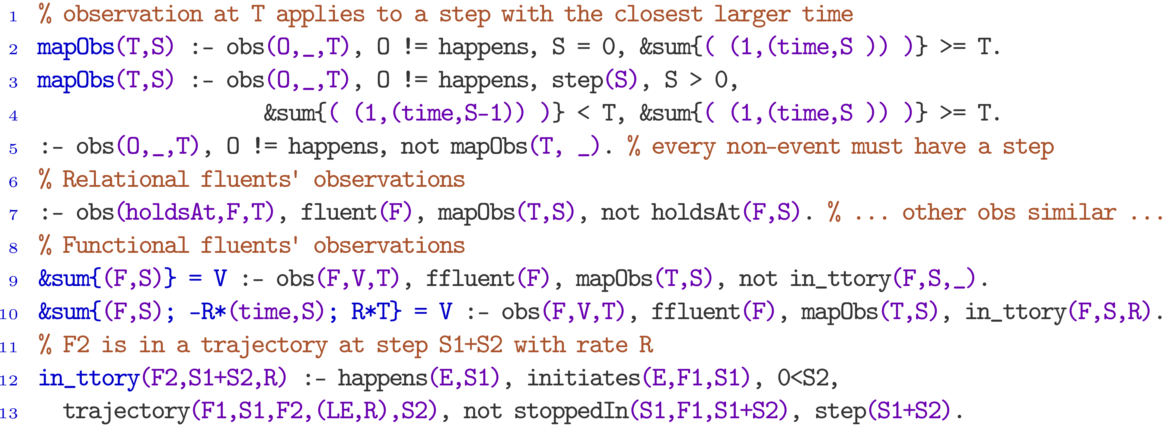
Figure 2 also shows how observations of event occurrences, which come as facts in the narrative of a problem instance, are mapped to time steps. An observation of an event $\color{blue}{\texttt{E}}$
at a timepoint
$\color{blue}{\texttt{E}}$
at a timepoint $\color{blue}{\texttt{T}}$
is represented by an atom
$\color{blue}{\texttt{T}}$
is represented by an atom $\color{blue}{\texttt{obs(happens,E,T)}}$
(see Section 4.4 for more details on observations). Lines 5–6 map timepoint
$\color{blue}{\texttt{obs(happens,E,T)}}$
(see Section 4.4 for more details on observations). Lines 5–6 map timepoint $\color{blue}{\texttt{T}}$
to some step
$\color{blue}{\texttt{T}}$
to some step $\color{blue}{\texttt{S}}$
, and line 7 derives the atom
$\color{blue}{\texttt{S}}$
, and line 7 derives the atom $\color{blue}{\texttt{happens(E,S)}}$
, which is used by the axioms introduced in the next section.
$\color{blue}{\texttt{happens(E,S)}}$
, which is used by the axioms introduced in the next section.
4.3 Modeling the axioms of hybrid EC
This section explains how we extend the DEC axioms as implemented by Lee and Palla (Reference Lee and Palla2012) to Hybrid EC. The extension builds on the previously defined functional fluents and the hybrid representation of time as discrete steps. This proposal provides a formal foundation for representing dense domains of fluents and time within a constraint-based framework, enabling a systematic encoding of axioms that support reasoning under Hybrid EC. The resulting axioms, referred to as HEC N (where N denotes the id of the corresponding DEC axiom), are summarized below:Footnote 5
-
HEC 1 redefines $\color{blue}{\texttt{stoppedIn}}$
as in DEC only for relational fluents.
$\color{blue}{\texttt{stoppedIn}}$
as in DEC only for relational fluents. -
HEC 2 extends
$\color{blue}{\texttt{startedIn}}$
for both types of fluents. -
HEC 3-4 capture the transition from gradual change of relational fluents to continuous change of functional fluents via
$\color{blue}{\texttt{trajectory}}$
/
$\color{blue}{\texttt{antiTrajectory}}$
. -
HEC 5 extends positive inertia for values of functional fluents and
$\color{blue}{\texttt{holdsAt}}$
of relational fluents. -
HEC 6 redefines negative inertia of
$\color{blue}{\texttt{holdsAt}}$
as in DEC only for relational fluents. -
HEC 7-8 redefines (the absence of)
$\color{blue}{\texttt{releasedAt}}$
capturing when any type of fluent is released or “un-released” from inertia by an event. -
HEC 9 extends positive effects of events via
$\color{blue}{\texttt{initiates}}$
for both types of fluents. -
HEC 10 redefines negative effects of events via
$\color{blue}{\texttt{terminates}}$
only for relational fluents. -
HEC 11-12 extends inertia for (the absence of)
$\color{blue}{\texttt{releasedAt}}$
for both types of fluents.





For brevity, we only focus on the implementation details of two most important sets of axioms: (1) In Section 4.3.1, we explain how to capture the effects of events and inertia on functional fluents. (2) In Section 4.3.2, we explain the transition from gradual change of relational fluents to continuous change of functional fluents.
4.3.1 Axioms for event effects and inertia
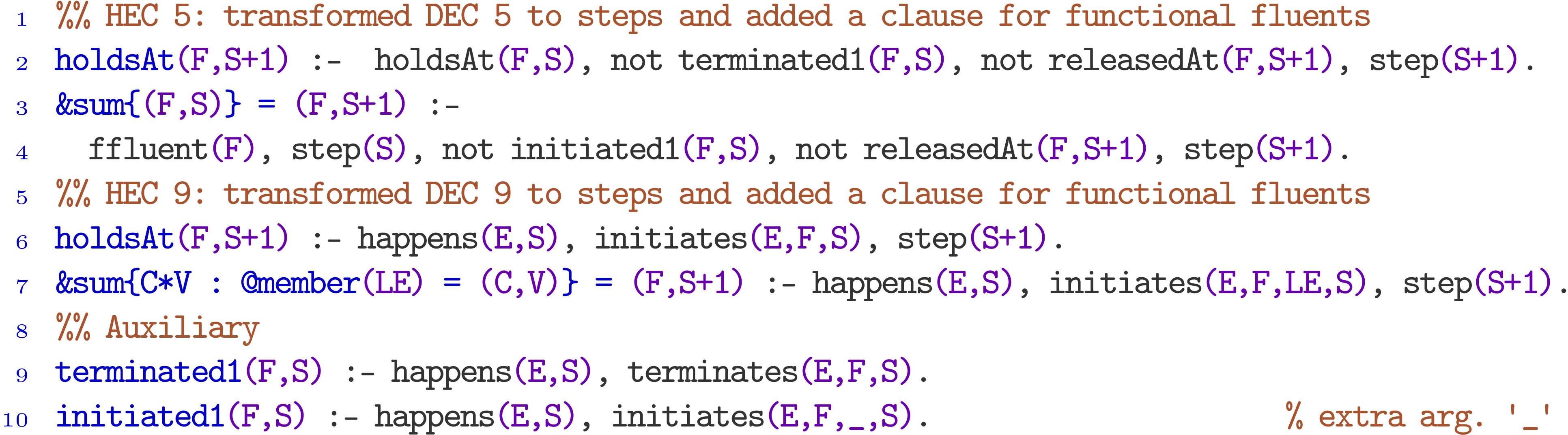
In DEC, a relational fluent starts to hold after being initiated by an event, ceases to hold when terminated by an event, or persists by inertia unless it is released. This behavior is encoded by Lee and Palla (Reference Lee and Palla2012) using axioms DEC 5-6 for inertia and axioms DEC 9-10 for event effects (DEC 5 and DEC 9 were shown in Figure 1c). In HEC, these axioms must be adapted to handle both relational and functional fluents (see Figure 3). For relational fluents, this adaptation is straightforward, as we simply replace predicate $\color{blue}{\texttt{time}}$
by
$\color{blue}{\texttt{time}}$
by $\color{blue}{\texttt{step}}$
(lines 2 and 6 of Figure 3).
$\color{blue}{\texttt{step}}$
(lines 2 and 6 of Figure 3).
Axioms of HEC 5 and HEC 9 representing event effects and inertia.

For functional fluents, the rule in lines 3–4 of HEC 5 represents inertia. The theory atom in the head assigns to fluent $\color{blue}{\texttt{F}}$
at step
$\color{blue}{\texttt{F}}$
at step $\color{blue}{\texttt{S+1}}$
the value of
$\color{blue}{\texttt{S+1}}$
the value of $\color{blue}{\texttt{F}}$
at step
$\color{blue}{\texttt{F}}$
at step $\color{blue}{\texttt{S}}$
unless the fluent is initiated or released from inertia. Line 7 of HEC 9 represents the effect of initiating fluent
$\color{blue}{\texttt{S}}$
unless the fluent is initiated or released from inertia. Line 7 of HEC 9 represents the effect of initiating fluent $\color{blue}{\texttt{F}}$
whenever event
$\color{blue}{\texttt{F}}$
whenever event $\color{blue}{\texttt{E}}$
happens at step
$\color{blue}{\texttt{E}}$
happens at step $\color{blue}{\texttt{S}}$
. The corresponding theory atom assigns to fluent
$\color{blue}{\texttt{S}}$
. The corresponding theory atom assigns to fluent $\color{blue}{\texttt{F}}$
at step
$\color{blue}{\texttt{F}}$
at step $\color{blue}{\texttt{S+1}}$
the value of the linear expression
$\color{blue}{\texttt{S+1}}$
the value of the linear expression $\color{blue}{\texttt{LE}}$
, given by a new predicate
$\color{blue}{\texttt{LE}}$
, given by a new predicate $\color{blue}{\texttt{initiates/4}}$
. A linear expression
$\color{blue}{\texttt{initiates/4}}$
. A linear expression $\color{blue}{{\texttt{c1*v1+}} \ldots \texttt{+cN*vN}}$
is encoded as a tuple
$\color{blue}{{\texttt{c1*v1+}} \ldots \texttt{+cN*vN}}$
is encoded as a tuple $\color{blue}{{{\texttt{((c1,v1)}}},\ldots ,\texttt{(cN,vN))}}$
,Footnote
6
which is unpacked by the Python external function
$\color{blue}{{{\texttt{((c1,v1)}}},\ldots ,\texttt{(cN,vN))}}$
,Footnote
6
which is unpacked by the Python external function $\color{blue}{\texttt{@member}}$
, yielding the set of theory elements
$\color{blue}{\texttt{@member}}$
, yielding the set of theory elements $\color{blue}{{\texttt{\{(c1*v1);}\ldots ;\texttt{(cN*vN)\}}}}$
. Rules for HEC 6 or HEC 10 about the termination of fluents are not needed, since functional fluents have exactly one value at every time step, and initiating a new value breaks the inertia of the previous value by deriving
$\color{blue}{{\texttt{\{(c1*v1);}\ldots ;\texttt{(cN*vN)\}}}}$
. Rules for HEC 6 or HEC 10 about the termination of fluents are not needed, since functional fluents have exactly one value at every time step, and initiating a new value breaks the inertia of the previous value by deriving $\color{blue}{\texttt{initiated1}}$
(line 10).
$\color{blue}{\texttt{initiated1}}$
(line 10).



4.3.2 Axioms for continuous change
Fluents in EC can undergo continuous change via trajectories and anti-trajectories. DEC can only model gradual change over discrete steps. In contrast, Hybrid EC supports reasoning about dense domains and can faithfully model continuous change, although it is limited to monotonic linear changes.
Figure 4(a) shows axiom DEC 3 for gradual change in DEC using trajectories. Figure 4(b) shows the corresponding rule HEC 3 for continuous change, which only applies to functional fluents as there are no trajectories for relational fluents in HEC. The representation of anti-trajectories in DEC 4 and HEC 4 is analogous, and we do not discuss it further. In HEC 3, the value of a functional fluent $\color{blue}{\texttt{F2}}$
at step
$\color{blue}{\texttt{F2}}$
at step $\color{blue}{\texttt{S1+S2}}$
is defined by a new predicate
$\color{blue}{\texttt{S1+S2}}$
is defined by a new predicate $\color{blue}{\texttt{trajectory(F1,S1,F2,(LE,R),S2)}}$
if an event
$\color{blue}{\texttt{trajectory(F1,S1,F2,(LE,R),S2)}}$
if an event $\color{blue}{\texttt{E}}$
initiated the relational fluent
$\color{blue}{\texttt{E}}$
initiated the relational fluent $\color{blue}{\texttt{F1}}$
at step
$\color{blue}{\texttt{F1}}$
at step $\color{blue}{\texttt{S1}}$
, and it has not been stopped since. The new atom over the predicate
$\color{blue}{\texttt{S1}}$
, and it has not been stopped since. The new atom over the predicate $\color{blue}{\texttt{trajectory}}$
specifies the value of
$\color{blue}{\texttt{trajectory}}$
specifies the value of $\color{blue}{\texttt{F2}}$
using the tuple
$\color{blue}{\texttt{F2}}$
using the tuple $\color{blue}{\texttt{(LE,R)}}$
. The linear expression
$\color{blue}{\texttt{(LE,R)}}$
. The linear expression $\color{blue}{\texttt{LE}}$
provides the value of
$\color{blue}{\texttt{LE}}$
provides the value of $\color{blue}{\texttt{F2}}$
at the beginning of the trajectory, and
$\color{blue}{\texttt{F2}}$
at the beginning of the trajectory, and $\color{blue}{\texttt{R}}$
gives the changing rate during the trajectory.Footnote
7
The new atom further refers to step
$\color{blue}{\texttt{R}}$
gives the changing rate during the trajectory.Footnote
7
The new atom further refers to step $\color{blue}{\texttt{S1}}$
and duration in steps
$\color{blue}{\texttt{S1}}$
and duration in steps $\color{blue}{\texttt{S2}}$
instead of timepoints. This is a key difference because the value assigned by the trajectory to
$\color{blue}{\texttt{S2}}$
instead of timepoints. This is a key difference because the value assigned by the trajectory to $\color{blue}{\texttt{F2}}$
cannot be derived directly from the step-based duration, as the result would vary if additional steps are inserted (e.g., due to an unrelated event occurring during the trajectory). Therefore, the theory atom in the head represents the linear expression
$\color{blue}{\texttt{F2}}$
cannot be derived directly from the step-based duration, as the result would vary if additional steps are inserted (e.g., due to an unrelated event occurring during the trajectory). Therefore, the theory atom in the head represents the linear expression $\color{blue}{\texttt{LE}}$
as in HEC 9 (unpacked by the function
$\color{blue}{\texttt{LE}}$
as in HEC 9 (unpacked by the function $\color{blue}{\texttt{@member}}$
) but further adds
$\color{blue}{\texttt{@member}}$
) but further adds $\color{blue}{\texttt{R*(time,S1+S2)}}$
and
$\color{blue}{\texttt{R*(time,S1+S2)}}$
and $\color{blue}{\texttt{-R*(time,S1)}}$
to encode the change
$\color{blue}{\texttt{-R*(time,S1)}}$
to encode the change $\color{blue}{\texttt{R*((time,S1+S2)-(time,S1))}}$
, which refers to the actual time difference between the concerned steps.
$\color{blue}{\texttt{R*((time,S1+S2)-(time,S1))}}$
, which refers to the actual time difference between the concerned steps.
Axioms for representing gradual (DEC) and continuous (HEC) change.

Example 4 (Falling Object, Example 2 cont.

 )
)
To show the transition from gradual to continuous change, we encode the trajectory of the falling object both in DEC and in HEC as follows: (see the full encoding in Appendix A.5)

The trajectory starts when the fluent $\color{blue}{\texttt{falling(O)}}$
is initiated by a
$\color{blue}{\texttt{falling(O)}}$
is initiated by a $\color{blue}{\texttt{drop(O)}}$
event, which also releases
$\color{blue}{\texttt{drop(O)}}$
event, which also releases $\color{blue}{\texttt{height(O)}}$
from inertia, and ends when
$\color{blue}{\texttt{height(O)}}$
from inertia, and ends when $\color{blue}{\texttt{falling(O)}}$
is terminated.
$\color{blue}{\texttt{falling(O)}}$
is terminated.
4.4 Modeling narratives in hybrid EC
A narrative of a problem instance consists of observations of event occurrences and fluent values. In HEC, observations are represented by facts of the form $\color{blue}{\texttt{obs(O1,O2,T)}}$
where
$\color{blue}{\texttt{obs(O1,O2,T)}}$
where $\color{blue}{\texttt{T}}$
denotes a timepoint:
$\color{blue}{\texttt{T}}$
denotes a timepoint: $\color{blue}{\texttt{obs(happens,E,T)}}$
for event occurrences,
$\color{blue}{\texttt{obs(happens,E,T)}}$
for event occurrences, $\color{blue}{\texttt{obs(holdsAt,F,T)}}$
and
$\color{blue}{\texttt{obs(holdsAt,F,T)}}$
and $\color{blue}{\texttt{obs(notHoldsAt,F,T)}}$
for values of relational fluents,
$\color{blue}{\texttt{obs(notHoldsAt,F,T)}}$
for values of relational fluents, $\color{blue}{\texttt{obs(F,Val,T)}}$
for values of functional fluents, and
$\color{blue}{\texttt{obs(F,Val,T)}}$
for values of functional fluents, and $\color{blue}{\texttt{obs(releasedAt,F,T)}}$
and
$\color{blue}{\texttt{obs(releasedAt,F,T)}}$
and $\color{blue}{\texttt{obs(notReleasedAt,F,T)}}$
for fluents released from inertia. We have already discussed event observations in Section 4.2. In this section, we focus on the representation of the other (fluent) observations.
$\color{blue}{\texttt{obs(notReleasedAt,F,T)}}$
for fluents released from inertia. We have already discussed event observations in Section 4.2. In this section, we focus on the representation of the other (fluent) observations.
The main task is to map observation timepoints to the steps used in HEC. Recall that fluents do not change between steps unless they are under the effect of a trajectory. As discussed in Section 4.2, the value of a fluent at step $\color{blue}{\texttt{S}}$
represents its value over the time interval
$\color{blue}{\texttt{S}}$
represents its value over the time interval $\color{blue}{\texttt{((time,S-1),(time,S)]}}$
. Hence, any observation at a timepoint within
$\color{blue}{\texttt{((time,S-1),(time,S)]}}$
. Hence, any observation at a timepoint within $\color{blue}{\texttt{((time,S-1),(time,S)]}}$
can be checked at step
$\color{blue}{\texttt{((time,S-1),(time,S)]}}$
can be checked at step $\color{blue}{\texttt{S}}$
. Based on this, the encoding maps timepoints to their corresponding steps and checks the observations on those steps. The mapping is defined in lines 2–5 of Figure 5 using predicate
$\color{blue}{\texttt{S}}$
. Based on this, the encoding maps timepoints to their corresponding steps and checks the observations on those steps. The mapping is defined in lines 2–5 of Figure 5 using predicate $\color{blue}{\texttt{mapObs(T,S)}}$
. The first rule covers the initial step, while the second rules handles the case where
$\color{blue}{\texttt{mapObs(T,S)}}$
. The first rule covers the initial step, while the second rules handles the case where $\color{blue}{\texttt{T}}$
falls within
$\color{blue}{\texttt{T}}$
falls within $\color{blue}{\texttt{((time,S-1),(time,S)]}}$
for
$\color{blue}{\texttt{((time,S-1),(time,S)]}}$
for
 . The constraint in line 7 uses this predicate to encode the observation of a relational fluent $\color{blue}{\texttt{F}}$
holding at timepoint
$\color{blue}{\texttt{F}}$
holding at timepoint $\color{blue}{\texttt{T}}$
. It forbids cases where
$\color{blue}{\texttt{T}}$
. It forbids cases where $\color{blue}{\texttt{T}}$
is mapped to step
$\color{blue}{\texttt{T}}$
is mapped to step $\color{blue}{\texttt{S}}$
but
$\color{blue}{\texttt{S}}$
but $\color{blue}{\texttt{F}}$
does not hold at
$\color{blue}{\texttt{F}}$
does not hold at $\color{blue}{\texttt{S}}$
. Other observations of relational fluents are encoded analogously.Footnote
8
$\color{blue}{\texttt{S}}$
. Other observations of relational fluents are encoded analogously.Footnote
8
Non-event observations.

For functional fluents, the auxiliary predicate
 , defined in lines 12–13, identifies the case where fluent $\color{blue}{\texttt{F}}$
is under a trajectory at step
$\color{blue}{\texttt{F}}$
is under a trajectory at step $\color{blue}{\texttt{S}}$
, and extracts the rate of change
$\color{blue}{\texttt{S}}$
, and extracts the rate of change $\color{blue}{\texttt{R}}$
. If no trajectory applies to
$\color{blue}{\texttt{R}}$
. If no trajectory applies to $\color{blue}{\texttt{F}}$
at step
$\color{blue}{\texttt{F}}$
at step $\color{blue}{\texttt{S}}$
, the situation is analogous to relational fluents, and line 9 checks the observed value of
$\color{blue}{\texttt{S}}$
, the situation is analogous to relational fluents, and line 9 checks the observed value of $\color{blue}{\texttt{F}}$
at the corresponding step
$\color{blue}{\texttt{F}}$
at the corresponding step $\color{blue}{\texttt{S}}$
. Otherwise, line 10 computes the value of
$\color{blue}{\texttt{S}}$
. Otherwise, line 10 computes the value of $\color{blue}{\texttt{F}}$
at the time
$\color{blue}{\texttt{F}}$
at the time $\color{blue}{\texttt{T}}$
of the observation as
$\color{blue}{\texttt{T}}$
of the observation as $\color{blue}{\texttt{(F,S)-R*((time,S)-T))}}$
, and checks it against the observed value
$\color{blue}{\texttt{(F,S)-R*((time,S)-T))}}$
, and checks it against the observed value $\color{blue}{\texttt{V}}$
.
$\color{blue}{\texttt{V}}$
.
Example 5 (Falling Object, Example 4 cont.

 )
)
Assume step $\color{blue}{\texttt{0}}$
is mapped to time
$\color{blue}{\texttt{0}}$
is mapped to time $\color{blue}{\texttt{10}}$
, step
$\color{blue}{\texttt{10}}$
, step $\color{blue}{\texttt{1}}$
is mapped to time
$\color{blue}{\texttt{1}}$
is mapped to time $\color{blue}{\texttt{20}}$
, object
$\color{blue}{\texttt{20}}$
, object $\color{blue}{\texttt{obj}}$
has height
$\color{blue}{\texttt{obj}}$
has height $\color{blue}{\texttt{20}}$
at step
$\color{blue}{\texttt{20}}$
at step $\color{blue}{\texttt{0}}$
, and height
$\color{blue}{\texttt{0}}$
, and height $\color{blue}{\texttt{0}}$
at step
$\color{blue}{\texttt{0}}$
at step $\color{blue}{\texttt{1}}$
. That is,
$\color{blue}{\texttt{1}}$
. That is, $\color{blue}{\texttt{(time,0)=10}}$
,
$\color{blue}{\texttt{(time,0)=10}}$
, $\color{blue}{\texttt{(time,1)=20}}$
,
$\color{blue}{\texttt{(time,1)=20}}$
, $\color{blue}{\texttt{(height(obj),0)=20}}$
, and
$\color{blue}{\texttt{(height(obj),0)=20}}$
, and $\color{blue}{\texttt{(height(obj),1)=0}}$
. Observation
$\color{blue}{\texttt{(height(obj),1)=0}}$
. Observation $\color{blue}{\texttt{obs(holdsAt,falling}}$ $\color{blue}{\texttt{(obj),15)}}$
holds because timepoint
$\color{blue}{\texttt{(obj),15)}}$
holds because timepoint $\color{blue}{\texttt{15}}$
is mapped to step
$\color{blue}{\texttt{15}}$
is mapped to step $\color{blue}{\texttt{1}}$
, and
$\color{blue}{\texttt{1}}$
, and $\color{blue}{\texttt{falling(obj)}}$
is true at that step. Indeed,
$\color{blue}{\texttt{falling(obj)}}$
is true at that step. Indeed, $\color{blue}{\texttt{obj}}$
is always falling during the time between steps
$\color{blue}{\texttt{obj}}$
is always falling during the time between steps $\color{blue}{\texttt{0}}$
and
$\color{blue}{\texttt{0}}$
and $\color{blue}{\texttt{1}}$
. Observation
$\color{blue}{\texttt{1}}$
. Observation $\color{blue}{\texttt{obs(height(obj),10,15)}}$
also holds. The height at step
$\color{blue}{\texttt{obs(height(obj),10,15)}}$
also holds. The height at step $\color{blue}{\texttt{1}}$
is
$\color{blue}{\texttt{1}}$
is $\color{blue}{\texttt{0}}$
, but the height at time
$\color{blue}{\texttt{0}}$
, but the height at time $\color{blue}{\texttt{15}}$
is
$\color{blue}{\texttt{15}}$
is $\color{blue}{\texttt{20-2*(20-15)=10}}$
due to the trajectory, which is consistent with the observation.
$\color{blue}{\texttt{20-2*(20-15)=10}}$
due to the trajectory, which is consistent with the observation.
4.5 Modeling triggered events in hybrid EC
Special considerations must be made for triggered events, that is, events whose occurrences are not given as observations in the narrative but rather implied by the rules of the domain description. For such events, there will be no mapping from observations to steps (Section 2). We handle triggered events by giving the reasoning extra free-floating steps that will not be mapped to an event occurrence observation. The event is triggered at one of the free-floating steps which is then assigned a time according to the evaluation of linear constraints defined in the trigger rule. However, additional constraints are needed in order to ensure that the step will not be placed at a different timepoint or that the step is not taken up by another triggered event that occurs later.
The
 constraint and a triggered event for the falling object.

The above is a common problem in hybrid systems and can be addressed using a constraint that prevents steps from jumping over particular values of interest when dealing with monotonic changes, as was discussed by Shin and Davis (Reference Shin and Davis2005) for SAT-based planning. In our case, this is relevant for events triggered based on continuous change of fluents or triggered after some delay. We define a predicate $\color{blue}{\texttt{no}\_\texttt{jump(Fluent, Step, Value)}}$
that introduces such a constraint for typical scenarios, as shown in Figure 6 (lines 1–2). The body of the rule that implies
$\color{blue}{\texttt{no}\_\texttt{jump(Fluent, Step, Value)}}$
that introduces such a constraint for typical scenarios, as shown in Figure 6 (lines 1–2). The body of the rule that implies $\color{blue}{\texttt{no}\_\texttt{jump}}$
should mirror the body of the trigger rule.
$\color{blue}{\texttt{no}\_\texttt{jump}}$
should mirror the body of the trigger rule.
The implicit last step (discussed in Section 4.2) is crucial to force the reasoning to check that the $\color{blue}{\texttt{no}\_\texttt{jump}}$
constraints are not violated after the last event occurrence (second to last step), which would signal the need for more steps.
$\color{blue}{\texttt{no}\_\texttt{jump}}$
constraints are not violated after the last event occurrence (second to last step), which would signal the need for more steps.
Example 6 (Falling Object, Example 5 cont.

 )
)
Consider, the falling object that is dropped from an initial height of 20 at time 10 and hits the ground when its height reaches zero. The observation of dropping the object and the triggered event of hitting the ground are encoded on lines 4–5 of Figure 6. This problem would need 3 steps in HEC: drop, hit the ground, and the last step. Reaching height zero is defined by the falling trajectory which in this case implies a trigger time of 20. Line 6 shows the necessary $\color{blue}{\texttt{no}\_\texttt{jump}}$
constraint saying that there must not exist two consecutive steps such that the height is less than zero at the first one and greater than zero at the second one, that is, one of the steps must have height exactly zero. Note that the object must be falling at the second step and not necessarily at the first step, as the value of a fluent at step
$\color{blue}{\texttt{no}\_\texttt{jump}}$
constraint saying that there must not exist two consecutive steps such that the height is less than zero at the first one and greater than zero at the second one, that is, one of the steps must have height exactly zero. Note that the object must be falling at the second step and not necessarily at the first step, as the value of a fluent at step $\color{blue}{\texttt{S}}$
represents the time period
$\color{blue}{\texttt{S}}$
represents the time period $\color{blue}{\texttt{((time,S-1),(time, S)]}}$
.
$\color{blue}{\texttt{((time,S-1),(time, S)]}}$
.
4.6 Incremental solving
Mapping time to steps (Section 4.2) requires at least as many steps as there are observations of event occurrences at distinct timepoints. However, it might be hard to know how many triggered events will occur in a particular problem instance. We have designed the axioms in such a way that the reasoning will only produce models for the right number of steps to cover all the events that occur from time zero to the time of the implicit last step, that is, there will be no models for not enough steps and for too many steps.
This is achieved by a combination of three techniques: (1) the implicit last step, (2) the $\color{blue}{\texttt{no}\_\texttt{jump}}$
constraints, and (3) a significant step constraint. The
$\color{blue}{\texttt{no}\_\texttt{jump}}$
constraints, and (3) a significant step constraint. The $\color{blue}{\texttt{no}\_\texttt{jump}}$
constraints and the implicit last step (Section 4.2) ensure that no models exist when too few steps are provided. To avoid excessive floating steps when too many steps are given, we introduce the constraint encoded in Figure 7 requiring all steps to be significant. A step is considered significant if it involves an event occurrence or if it is the last step.
$\color{blue}{\texttt{no}\_\texttt{jump}}$
constraints and the implicit last step (Section 4.2) ensure that no models exist when too few steps are provided. To avoid excessive floating steps when too many steps are given, we introduce the constraint encoded in Figure 7 requiring all steps to be significant. A step is considered significant if it involves an event occurrence or if it is the last step.
The significant step constraint.

Our implementation uses an incremental execution approach to find the right number of steps automatically. A limitation of this approach is that it currently is not possible to automatically identify that there is no model for any number of steps. Instead, the script currently explores up to a given maximum number of steps as defined by the user.
5 Accurately representing continuous change
The use of integer time and values of fluents in DEC means that it cannot model continuous change. Instead, it models gradual change which can lead to inaccurate representation.
Example 7 (Falling Object, Example 6 cont.

 )
)
Consider the falling object. If it is dropped from height 20 at time 10 and falls via a constant speed of 2 units, then it will hit the ground at time 20 with height 0. However, if it was dropped from height 21, then its height would be 1 at time 20 and –1 at time 21, that is, there would be no integer time at which the height is equal to zero.
This problem can be mitigated on a case-by-case basis by approximation (e.g., triggering before or after stepping over height zero), which leads to inaccurate representation, or by increasing the precision of the discretization (e.g., multiplying the time and height by a factor of 10), which can quickly lead to very large value domains. Although a large value domain is no longer a problem for HEC with clingcon, it can be difficult or impossible to identify how fine the discretization needs to be for some problem instances.
Since HEC reasons about values of functional fluents and time using theory atoms, we can switch to reasoning using dense values instead of integers, which would be impossible without the hybrid approach. We can do this by simply replacing clingcon with clingo-lpx, which reasons about theory atoms in the domain of rational numbers (see Section 2.2).
However, one must consider the challenges that come with reasoning in dense time, such as Zeno behavior and various Zeno-like phenomena, whose causes in EC were studied by Vašíček et al. (Reference Vašíček, Arias, Fiedor, Gupta, Hall, Křena, Larson and Vojnar2025). For example, preventing the repeated triggering of events, a basic modeling technique for ensuring that an event is only triggered once after its trigger condition starts to hold, becomes a fundamental problem because one may end up reasoning about the smallest timepoint $\color{blue}{\texttt{T2}}$
such that
$\color{blue}{\texttt{T2}}$
such that $\color{blue}{\texttt{T2}\,\gt\,\texttt{T1}}$
for some given timepoint
$\color{blue}{\texttt{T2}\,\gt\,\texttt{T1}}$
for some given timepoint $\color{blue}{\texttt{T1}}$
, with no such
$\color{blue}{\texttt{T1}}$
, with no such $\color{blue}{\texttt{T2}}$
existing in a dense domain. These challenges can be addressed using the techniques proposed by Vašíček et al. (Reference Vašíček, Arias, Fiedor, Gupta, Hall, Křena, Larson and Vojnar2025). Although a detailed discussion of this in the context of HEC is outside the scope of this paper and left for future work, we provide encodings of four such problems (listed in Appendix A.1).
$\color{blue}{\texttt{T2}}$
existing in a dense domain. These challenges can be addressed using the techniques proposed by Vašíček et al. (Reference Vašíček, Arias, Fiedor, Gupta, Hall, Křena, Larson and Vojnar2025). Although a detailed discussion of this in the context of HEC is outside the scope of this paper and left for future work, we provide encodings of four such problems (listed in Appendix A.1).
6 Experimental evaluation
The key features to evaluate for Hybrid EC are: (1) its expressive power to encode and reason about continuous change in EC, and (2) improvements in time and memory scalability, particularly, with respect to the size of the time and fluent value domains.
6.1 Expressiveness
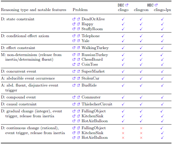
We used HEC to encode benchmark problems from the works by Mueller (Reference Mueller2004) and Lee and Palla (Reference Lee and Palla2012), additional problems from the works by Mueller (Reference Mueller2008, Reference Mueller2014), relevant problems from the work by Vašíček et al. (Reference Vašíček, Arias, Fiedor, Gupta, Hall, Křena, Larson and Vojnar2025), and some modifications to highlight the benefits of using HEC under rationals. The implementations for clingo, clingcon, and clingo-lpx of over 30 problems are available at https://github.com/ovasicek/hybrid-ec and archived at
 ; for brevity, Table 2 lists only a subset (the full table is available in Appendix A.1). The problems considered illustrate the modeling and reasoning capabilities of the compared approaches. They are grouped by their most notable features, including the reasoning mode they use, with two examples showcasing abductive reasoning. Classification of features and reasoning follows the one used by Mueller (Reference Mueller2004, Reference Mueller2014). The table confirms that HEC with both clingcon and clingo-lpx can reason about all the examples that DEC with clingo handles. In addition, the use of rationals in clingo-lpx allows us to accurately reason about problems that require continuous change, that is, dense domains for time and fluent values, which is not possible with clingo and neither with clingcon.
Comparing the expressiveness of DEC and HEC

Reasoning types: D = deduction, M = model finding, A = abduction.
6.2 Performance
We now present two experiments performed on an AMD EPYC 9124 CPU (base clock of 3 GHz), measuring execution times and memory usage averaged over 10 runs with a timeout of 300 s while finding all models.Footnote 9
a) Domain size: Figure 8a shows the execution time scaling for clingo, clingcon, and clingo-lpx with the domain size (time and values of fluents) using problems from the work by Lee and Palla (Reference Lee and Palla2012) and Example 1 the counter (full encoding is available in Appendix A.4). For plain ASP (clingo), we highlight problems that feature fluents with numerical values using purple lines since for these, the domain size increases not only in time but also in values of the fluents. The two blue lines that reach a timeout correspond to the StolenCar and the ThielscherCircuit (detailed Figures are available in Appendix A.3). The results show that the domain size indeed does not affect the Hybrid ASP execution at all, while plain ASP does not scale. This is a great advantage of using the hybrid approach, since plain ASP is fundamentally not equipped to handle large domains which greatly limits its usability in reasoning about requirements specifications of CPSs. The memory usage scaling looks very similar to the execution time scaling with the hybrid approach using up to 30 MB, and plain ASP using up to 50 GB for the curves that reach the timeout and up to 1 GB for the others (see Figure 1 of Appendix A.2).
(a) Scaling with the size of the domain, (b) Scaling with the number of events.

b) Number of events: To measure the impact of including more events, we use Example 2 the falling object (full encoding is available in Appendix A.5), increasing the number of times the object is dropped. Figure 8b shows the execution time scaling with the number of events, which is particularly relevant for evaluating the scalability of Hybrid ASP solvers, as an increasing number of events raises both the grounding size (number of steps in HEC) and the complexity of the reasoning. For clingcon and clingo-lpx, we report (i) the cost of an incremental evaluation to determine the correct number of steps to model the problem and (ii) a single evaluation using the correct (guessed) number of steps. The resulting measurements show that clingo-lpx is slower than clingcon but overall scales similarly, meaning that the introduction of rationals does not significantly impact scaling. In addition, the incremental execution approach shows scaling similar to that of guessing the right number of steps. The memory usage scaling again looks similar to the execution time scaling with the maximum reaching around 300 MB. A notable difference is that clingo-lpx only uses more memory than clingcon for up to around 30 events and uses less from then on (see Figure 2 of Appendix A.2).
Clearly, unlike the domain size, the number of events does have a significant impact on the hybrid approach, which is complementary to the results of clingo (not shown in the graph not to clutter it too much), on which the number of events has almost no impact since the domain size remains unchanged. However, we note that, in the context of high-level requirements specifications of CPSs, it is often much more important to be able to handle large domains and accurately represent continuous behavior rather than to represent large numbers of events. Indeed, many errors can be detected within relatively short narratives corresponding to use cases described as a part of the specification as shown, for example in the work by Vašíček et al. (Reference Vašíček, Arias, Fiedor, Gupta, Hall, Křena, Larson, Varanasi and Vojnar2024), while restricting the domain or discretization can lead to missing the error. Finally, we note that, compared to s(CASP), the hybrid approach provides a significant speedup since s(CASP) reaches the timeout on the problem considered in Figure 8 at already eight events.
7 Conclusion
We have presented Hybrid EC, an encoding of the EC for Hybrid ASP solvers based on DEC, and its implementation in HEC axioms. The resulting framework combines ASP with linear constraints (over integers and/or rationals) that effectively avoids the grounding bottleneck when the domain of time and fluent values increases, as well as the problem of inaccurate modeling due to discretization when reasoning considering continuous changes (requiring dense domains). We have shown both of these advantages on a number of problems from the literature and provide all their encodings as modeling guides at https://github.com/ovasicek/hybrid-ec
 .
.
This work opens several lines for future research, for example: using HEC to analyze real-life CPS specifications as done with s(CASP) for the PCA pump specification in the work by Vašíček et al. (Reference Vašíček, Arias, Fiedor, Gupta, Hall, Křena, Larson, Varanasi and Vojnar2024), hopefully avoiding some of the scalability/termination barriers hit with s(CASP); a deeper comparison of HEC for clingo-lpx against s(CASP) and other Hybrid ASP solvers; utilization of clingo’s multi-shot solving for more efficiency; improving the syntax of HEC (especially nested tuples); and finally, application of HEC on planning problems in the general-purpose definition language PDDL.
Supplementary material
To view supplementary material for this article, please visit https://doi.org/10.1017/S147106842610060X














 Open access

