


1 INTRODUCTION AND MOTIVATION
Asset price bubbles tend to be characterized by a sudden and explosive increase in the price of an asset without a corresponding increase in the fundamental value of the asset (thereby representing a misallocation of resources), followed by a subsequent destruction of value through a price collapse. Bubbles often presage economic recessions; indeed, the 2007/08 Global Financial Crisis (GFC) was preceded by suspected price bubbles in the U.S. housing, commodity, and stock markets. In the aftermath of the GFC, policymakers have considered new rules for macroprudential regulation and intervention. Crucial to the effectiveness of these is the availability of econometric methods which can monitor the behavior of prices in asset markets in real time, rapidly and accurately detecting emerging price bubbles.
The majority of the bubble detection literature has focused on one-shot tests for detecting the presence of historic asset price bubbles. The seminal contributions in this area were made by Phillips, Wu, and Yu (Reference Phillips, Wu and Yu2011) [PWY] and Phillips, Shi, and Yu (Reference Phillips, Shi and Yu2015) [PSY], who proposed tests for the presence of bubble episodes based on the maximum of sequences of recursive univariate augmented Dickey–Fuller (ADF) unit root statistics applied to overlapping subsamples of the data. Other contributions based on subsample-based methods include: Homm and Breitung (Reference Homm and Breitung2012) [HB], Harvey et al. (Reference Harvey, Leybourne, Sollis and Taylor2016), Astill et al. (Reference Astill, Harvey, Leybourne and Taylor2017), Phillips and Shi (Reference Phillips and Shi2018), and Harvey, Leybourne, and Zu (Reference Harvey, Leybourne and Zu2019, Reference Harvey, Leybourne and Zu2020).
Although primarily designed as one-shot tests and date-stamping procedures for historical bubbles, some of these approaches can also be implemented sequentially to provide methods to monitor for the emergence of a bubble in real time; most notably the $BSADF$
statistic of PSY (defined as the maximum of a backward-recursive sequence of subsample ADF statistics computed over all possible subsamples ending at the last available date in the full data sample, subject to a minimum subsample length). By implementing tests sequentially, however, a critical value which diverges with the sample size (satisfying the rate condition given in Equation (11) on page 1055 of PSY), needs to be used to control the false positive rate (FPR) of the monitoring procedure, defined as the probability of incorrectly declaring a bubble during the monitoring period (see Section 3.2 of PSY). This rate condition implies a theoretical FPR (by which we mean the FPR of the procedure in large samples) of zero. In practice, PSY (p. 1066) recommend obtaining the critical value by Monte Carlo simulation, yielding a real-time monitoring procedure with a controlled, but nonzero, FPR. This procedure is, however, infeasible in the case where the innovations display time-varying volatility. To allow for possible time-varying volatility, Phillips and Shi (Reference Phillips and Shi2020, Sect. 5) propose a wild bootstrap monitoring procedure, based on the
$BSADF$
statistic of PSY (defined as the maximum of a backward-recursive sequence of subsample ADF statistics computed over all possible subsamples ending at the last available date in the full data sample, subject to a minimum subsample length). By implementing tests sequentially, however, a critical value which diverges with the sample size (satisfying the rate condition given in Equation (11) on page 1055 of PSY), needs to be used to control the false positive rate (FPR) of the monitoring procedure, defined as the probability of incorrectly declaring a bubble during the monitoring period (see Section 3.2 of PSY). This rate condition implies a theoretical FPR (by which we mean the FPR of the procedure in large samples) of zero. In practice, PSY (p. 1066) recommend obtaining the critical value by Monte Carlo simulation, yielding a real-time monitoring procedure with a controlled, but nonzero, FPR. This procedure is, however, infeasible in the case where the innovations display time-varying volatility. To allow for possible time-varying volatility, Phillips and Shi (Reference Phillips and Shi2020, Sect. 5) propose a wild bootstrap monitoring procedure, based on the $BSADF$
statistic, whose FPR can be controlled at a specified level across a monitoring period of a given length. This procedure is implemented at the end of the chosen monitoring period, and so is not run in real time; it may, however, be possible to modify this procedure to be implemented in real time.
$BSADF$
statistic, whose FPR can be controlled at a specified level across a monitoring period of a given length. This procedure is implemented at the end of the chosen monitoring period, and so is not run in real time; it may, however, be possible to modify this procedure to be implemented in real time.
A different strand of the literature, which we focus on in this article, has developed dedicated real-time monitoring procedures for asset price bubbles, designed so that the practitioner can fix the theoretical FPR at a given (nonzero) level. These split the data into a training sample and a monitoring period. HB use a CUSUM-based detector where a sequence of CUSUM statistics, calculated from the first differences of the data in real time over the monitoring period, are compared against a theoretical crossing function (such that the critical value becomes larger the further into the monitoring sequence one is). In a different approach, Astill et al. (Reference Astill, Harvey, Leybourne, Sollis and Taylor2018) use a method based on comparing the maximum value of statistics computed in the training sample and monitoring period. Both of these procedures are designed for the case where the innovations are unconditionally homoskedastic and assume that no relevant covariates exist. To deal with the first issue, Astill et al. (Reference Astill, Harvey, Leybourne, Taylor and Zu2023a) [AHLTZ] propose standardizing the CUSUM statistics used in the HB procedure by a nonparametric kernel-based spot variance estimator at each monitoring point. They show that a monitoring procedure based on these standardized CUSUM statistics has a theoretically controlled FPR even where the innovations are unconditionally heteroskedastic. As we will show, failure to account for relevant dynamic covariates in the data generating process (DGP) can lead to spurious over-rejection in both the HB and AHLTZ procedures.
It seems eminently plausible that information additional to the asset price series under test could usefully be deployed in bubble detection methods. Indeed, the literature suggests several potential covariates that might aid in identifying periods of explosive behavior. For equities, dividend discount type models (Diba and Grossman, 1998; PSY) link prices to the risk-free rate of interest, while the capital asset pricing model (Kim and Kim, Reference Kim and Kim2016) can embed time-varying volatility. Pricing equations for commodity spot prices (Tsvetanov, Coakley, and Kellard, Reference Tsvetanov, Coakley and Kellard2016) indicate that inventories (Kilian and Murphy, Reference Kilian and Murphy2014) play a role. Finally, given bubble behavior in real estate may precede equity (Caballero, Farhi, and Gourinchas, Reference Caballero, Farhi and Gourinchas2008) and commodity market bubbles (Phillips and Yu, Reference Phillips and Yu2011), potential housing market covariates, such as interest rates, disposable income, and mortgage finance (White, Reference White2015), may be particularly useful.
Despite these considerations, the majority of contributions in the bubble testing literature, and all of those described above, are purely univariate, using information from the price series under consideration alone. Two notable exceptions are Shi and Phillips (Reference Shi and Phillips2023) and Astill et al. (Reference Astill, Taylor, Kellard and Korkos2023b) [ATKK]. In the context of detecting house price bubbles, Shi and Phillips (Reference Shi and Phillips2023) develop $BSADF$
-type statistics applied to the (cumulated) residuals from a first-stage IVX regression (see, e.g., Kostakis et al., Reference Kostakis, Magdalinos and Stamatogiannis2015) which filters out market fundamentals from an observed price-to-rent series and use these in a monitoring procedure based on the approach of Phillips and Shi (Reference Phillips and Shi2020), discussed above. More relevant to the present setting, ATKK adapt the covariate ADF (CADF) unit root test proposed by Hansen (Reference Hansen1995) to develop versions of the historical bubble testing procedures of PWY and PSY, allowing information from covariates to be exploited. Hansen (Reference Hansen1995) shows that the inclusion of relevant (stationary) covariates in the CADF regression reduces the error variance relative to a univariate ADF regression and so can lead to more precise estimation of the model. ATKK show that the resulting covariate-augmented variants of the PWY and PSY tests can in some cases display significantly higher power to detect historical asset prices bubbles than their univariate counterparts from PWY and PSY.
$BSADF$
-type statistics applied to the (cumulated) residuals from a first-stage IVX regression (see, e.g., Kostakis et al., Reference Kostakis, Magdalinos and Stamatogiannis2015) which filters out market fundamentals from an observed price-to-rent series and use these in a monitoring procedure based on the approach of Phillips and Shi (Reference Phillips and Shi2020), discussed above. More relevant to the present setting, ATKK adapt the covariate ADF (CADF) unit root test proposed by Hansen (Reference Hansen1995) to develop versions of the historical bubble testing procedures of PWY and PSY, allowing information from covariates to be exploited. Hansen (Reference Hansen1995) shows that the inclusion of relevant (stationary) covariates in the CADF regression reduces the error variance relative to a univariate ADF regression and so can lead to more precise estimation of the model. ATKK show that the resulting covariate-augmented variants of the PWY and PSY tests can in some cases display significantly higher power to detect historical asset prices bubbles than their univariate counterparts from PWY and PSY.
Given the policy need for real-time monitoring procedures that can detect emerging bubbles as rapidly as possible, the findings in ATKK suggest that it is worth exploring if the incorporation of additional information from covariates can both improve the efficacy of real-time bubble monitoring procedures to detect emerging bubble episodes, while also delivering a controlled FPR under the null. Motivated by the CUSUM approach of Kramer, Ploberger, and Alt (Reference Kramer, Ploberger and Alt1988) [KPA], developed for detecting structural changes in dynamic models, we propose the CUSUM type real-time monitoring statistics based on recursive residuals from a regression of the first differences of the price series under test on relevant covariates. Like AHLTZ, we implement the procedures using a nonparametric kernel-based spot variance estimator at each time point to allow for time-varying volatility in the innovations. We also allow for serial correlation in the innovations, something also not allowed under the assumptions in HB.
We demonstrate that the resulting CUSUM statistic retains the same (pivotal) limiting distribution under the constant parameter unit root null as HB’s original CUSUM statistic attains under the regularity conditions in their paper. Consequently, a covariate-augmented monitoring procedure with a theoretically controlled FPR can be constructed by appealing to large sample results from Chu, Stinchcombe, and White (Reference Chu, Stinchcombe and White1996). Monte Carlo simulations show that for a wide range of potential DGPs our proposed covariate-augmented CUSUM monitoring procedure, implemented using a standard BIC criterion to decide whether or not to include a candidate covariate, performs well in practice. In particular, and unlike the univariate CUSUM-based monitoring procedures, the finite sample FPRs of the covariate-augmented procedures are well controlled when a genuine covariate is present in the DGP. Moreover, where the covariate enters the DGP, the true positive rate (TPR), defined as the cumulative probability of detecting a bubble present in the monitoring period, is much superior to the univariate procedures. Additionally, the impact on finite sample performance is very small in the case where the candidate covariate does not enter the DGP.
The remainder of the article is organized as follows. Section 2 outlines the DGP we work with and the assumptions under which we will operate. Section 3 gives a brief description of the standard CUSUM procedure of HB. Section 4 outlines our proposed covariate-augmented CUSUM monitoring procedure for covariates that are allowed to have nonzero means and details its large sample behavior. The results from our Monte Carlo simulation study are reported in Section 5. Section 6 concludes. The Supplementary Material details: the analogous procedure for the case where it is known that the covariates are mean zero; proofs of the technical results given in the article; additional simulation results; and an empirical illustration using the dataset of Welch and Goyal (Reference Welch and Goyal2008).
2 THE MODEL AND ASSUMPTIONS
Let $\{y_t\}$
be generated according to the following DGP:
$\{y_t\}$
be generated according to the following DGP:
 $$ \begin{align} y_t & = \mu^*+u_t \end{align} $$
 $$ \begin{align} u_t & = \left\{\begin{array}{@{}ll} u_{t - 1} + v_t & t = 1, \dots, \lfloor \tau T \rfloor\\ (1 + \delta) u_{t - 1} + v_t & t = \lfloor \tau T \rfloor + 1, \dots, \lfloor \lambda T \rfloor, \end{array}\right. \end{align} $$
where $1 \leq \tau \leq \lambda $
,
$1 \leq \tau \leq \lambda $
, $\lambda>1$
and
$\lambda>1$
and $\lfloor. \rfloor $
denotes the integer part of its argument. The initial condition
$\lfloor. \rfloor $
denotes the integer part of its argument. The initial condition $u_0$
is assumed to be of
$u_0$
is assumed to be of $O_p(1) $
. Under (2),
$O_p(1) $
. Under (2), $u_t$
follows the time-varying AR(1) process
$u_t$
follows the time-varying AR(1) process
 $$ \begin{align} \Delta u_t = \delta_t u_{t - 1} + v_t , \; \; t = 1, \ldots, T, \dots, \lfloor \lambda T \rfloor, \end{align} $$
where $\Delta := (1-L) $
is the usual first difference operator in the lag operator, L. The AR coefficient
$\Delta := (1-L) $
is the usual first difference operator in the lag operator, L. The AR coefficient $\delta _t$
can be seen to change from 0 to
$\delta _t$
can be seen to change from 0 to $\delta \geq 0$
at time
$\delta \geq 0$
at time $t= \lfloor \tau T \rfloor +1$
.
$t= \lfloor \tau T \rfloor +1$
.
In the context of (1) and (2), we will be concerned with two subsample periods of the series $y_{t}$
. The first of these is the period
$y_{t}$
. The first of these is the period $t=1,\ldots ,T$
, which will form the training sample in our analysis, and the second is the period
$t=1,\ldots ,T$
, which will form the training sample in our analysis, and the second is the period $t=T+1,\dots ,\lfloor \lambda T\rfloor $
, which will form the monitoring period for our procedure. Our model imposes that
$t=T+1,\dots ,\lfloor \lambda T\rfloor $
, which will form the monitoring period for our procedure. Our model imposes that $y_{t}$
follows a unit root process over the training sample
$y_{t}$
follows a unit root process over the training sample $t=1,\ldots ,T$
, while over the monitoring period
$t=1,\ldots ,T$
, while over the monitoring period $y_{t}$
again follows a unit root process over the sub-period
$y_{t}$
again follows a unit root process over the sub-period ${t=T+1,\dots ,\lfloor \tau T\rfloor }$
, but crucially is subject to potentially explosive behavior in the period
${t=T+1,\dots ,\lfloor \tau T\rfloor }$
, but crucially is subject to potentially explosive behavior in the period $t=\lfloor \tau T\rfloor +1,\dots ,\lfloor \lambda T\rfloor $
if
$t=\lfloor \tau T\rfloor +1,\dots ,\lfloor \lambda T\rfloor $
if $\delta>0$
.Footnote
1
In total, at the end of the monitoring period, there are
$\delta>0$
.Footnote
1
In total, at the end of the monitoring period, there are $ \lfloor \lambda T\rfloor $
observations. When
$ \lfloor \lambda T\rfloor $
observations. When $\delta> 0 $
, if
$\delta> 0 $
, if $\tau =1,$
then the explosive regime will begin at the start of the monitoring period. In the context of monitoring for explosive autoregressive behavior during the monitoring period, our implicit null hypothesis is given by
$\tau =1,$
then the explosive regime will begin at the start of the monitoring period. In the context of monitoring for explosive autoregressive behavior during the monitoring period, our implicit null hypothesis is given by $H_{0}:\delta = 0$
, with the corresponding alternative hypothesis,
$H_{0}:\delta = 0$
, with the corresponding alternative hypothesis, $H_{1}:\delta>0$
.
$H_{1}:\delta>0$
.
With respect to the error process, $v_t$
, in (2), we allow
$v_t$
, in (2), we allow $v_t$
to be serially correlated, heteroskedastic and (potentially) related to an
$v_t$
to be serially correlated, heteroskedastic and (potentially) related to an $ (m \times 1 )$
vector of covariates,
$ (m \times 1 )$
vector of covariates, $x_t$
. In the same spirit as Hansen (Reference Hansen1995), we achieve this by assuming that
$x_t$
. In the same spirit as Hansen (Reference Hansen1995), we achieve this by assuming that $v_t$
satisfies Assumption 1.
$v_t$
satisfies Assumption 1.
Assumption 1. Let ${v}_t$
be generated by the pth-order heteroskedastic autoregressive exogenous [
${v}_t$
be generated by the pth-order heteroskedastic autoregressive exogenous [ $ARX(p)$
] process
$ARX(p)$
] process
 $$ \begin{align} \alpha (L) v_t = \beta (L)' [ x_t - c_x ] +\varepsilon_t, \quad \varepsilon_t = \sigma_t \eta_t , \end{align} $$
where $\alpha (z) := 1 - \sum _{k = 1}^p \alpha _k z^k$
,
$\alpha (z) := 1 - \sum _{k = 1}^p \alpha _k z^k$
, $\beta (z) := \sum _{k = 0}^q \beta _k z^k$
, and where
$\beta (z) := \sum _{k = 0}^q \beta _k z^k$
, and where $x_t := ( x_{1,t},\ldots ,x_{m,t} )^\prime $
is an m-vector of stochastic covariates with constant mean vector
$x_t := ( x_{1,t},\ldots ,x_{m,t} )^\prime $
is an m-vector of stochastic covariates with constant mean vector $ c_x$
. Let the mean-centered vector of covariates be denoted
$ c_x$
. Let the mean-centered vector of covariates be denoted $ w_t := x_t - c_x =: (w_{1,t},\ldots , w_{m,t})^\prime $
. The innovations,
$ w_t := x_t - c_x =: (w_{1,t},\ldots , w_{m,t})^\prime $
. The innovations, $\eta _t$
, form a sequence of serially uncorrelated conditionally heteroskedastic innovations with mean zero and unit (unconditional) variance, with
$\eta _t$
, form a sequence of serially uncorrelated conditionally heteroskedastic innovations with mean zero and unit (unconditional) variance, with $ \sigma _t$
a (deterministic) time-varying volatility function, such that
$ \sigma _t$
a (deterministic) time-varying volatility function, such that $ \varepsilon _t $
has time-varying unconditional variance,
$ \varepsilon _t $
has time-varying unconditional variance, $\sigma _t^2$
.
$\sigma _t^2$
.
Remark 2.1. In (4), the lag polynomial $\beta (L)$
allows for, but does not require, lags of the covariate
$\beta (L)$
allows for, but does not require, lags of the covariate $x_t $
to enter the DGP. Compared to Equation (5) of Hansen (Reference Hansen1995, p. 1150),
$x_t $
to enter the DGP. Compared to Equation (5) of Hansen (Reference Hansen1995, p. 1150), $\beta (L) $
, however, excludes the possibility of leads of the covariate entering (4). This is a consequence of the fact that our interest in this article is on developing real-time monitoring procedures, whereby lead variables would be unavailable to the practitioner (see also Remark 4.1 of ATKK [p. 347]). Notice that the variables in
$\beta (L) $
, however, excludes the possibility of leads of the covariate entering (4). This is a consequence of the fact that our interest in this article is on developing real-time monitoring procedures, whereby lead variables would be unavailable to the practitioner (see also Remark 4.1 of ATKK [p. 347]). Notice that the variables in $x_t$
are not relevant covariates if
$x_t$
are not relevant covariates if $ \beta (L) = {0} $
.
$ \beta (L) = {0} $
.
Remark 2.2. Following the bulk of the econometric bubble detection literature, we model asset prices with the time-varying AR model in (1) and (2). As discussed in PWY and Breitung and Kruse (Reference Breitung and Kruse2013), inter alia, this is often motivated as an approximation to the rational bubble model where the observed asset price, $y_t$
, is equal to the sum of the fundamental price,
$y_t$
, is equal to the sum of the fundamental price, $ f_t$
, of the asset, assumed to be a martingale (
$ f_t$
, of the asset, assumed to be a martingale ( $I(1)$
) process, and a bubble component,
$I(1)$
) process, and a bubble component, $B_t$
, which is zero other than in its bubble phase when it is a submartingale (explosive
$B_t$
, which is zero other than in its bubble phase when it is a submartingale (explosive $AR(1)$
process). Under Assumption 1, the error term,
$AR(1)$
process). Under Assumption 1, the error term, $v_t$
, in (1) and (2) is related to a set of covariates. This therefore entails the implicit assumption that the covariates would be related to both
$v_t$
, in (1) and (2) is related to a set of covariates. This therefore entails the implicit assumption that the covariates would be related to both $f_t$
and
$f_t$
and $B_t$
in the rational bubble model. It is, however, possible that a given covariate could be related to only the error term driving one of these components. If this were the bubble component then, as noted by a referee, we would not expect any power gains from incorporating that covariate into the CUSUM bubble detection procedure.
$B_t$
in the rational bubble model. It is, however, possible that a given covariate could be related to only the error term driving one of these components. If this were the bubble component then, as noted by a referee, we would not expect any power gains from incorporating that covariate into the CUSUM bubble detection procedure.
Under the null hypothesis $H_0 : \delta = 0$
, we have that
$H_0 : \delta = 0$
, we have that $\Delta y_t = v_t$
for the full sample period
$\Delta y_t = v_t$
for the full sample period $t = 1, \dots , \lfloor \lambda T \rfloor $
, and so, from (4), we then have that
$t = 1, \dots , \lfloor \lambda T \rfloor $
, and so, from (4), we then have that
 $$ \begin{align} \Delta y_t = \mu + \sum_{k = 1}^p \alpha_k \Delta y_{t - k} + \sum_{k = 0}^q \beta_k' {x}_{t - k} + \varepsilon_t, \end{align} $$
where $ \mu := - \sum _{k=0}^q \beta _k^\prime c_x $
and where the first summation term is understood to be present only when
$ \mu := - \sum _{k=0}^q \beta _k^\prime c_x $
and where the first summation term is understood to be present only when $p>0$
. Notice that the intercept term
$p>0$
. Notice that the intercept term $ \mu =0 $
if either
$ \mu =0 $
if either $ c_x = 0 $
, such that the covariates have mean zero, or
$ c_x = 0 $
, such that the covariates have mean zero, or $\beta (L) = 0 $
, such that
$\beta (L) = 0 $
, such that $x_t $
are not relevant covariates.Footnote
2
This is a heteroskedastic autoregressive model in
$x_t $
are not relevant covariates.Footnote
2
This is a heteroskedastic autoregressive model in $\Delta y_t$
augmented by the level and (up to) q lags of the m covariates. Defining
$\Delta y_t$
augmented by the level and (up to) q lags of the m covariates. Defining ${g}_t: = (1, \Delta y_{t - 1}, \dots , \Delta y_{t - p}, x_{t'} ,x_{t - 1'}, \ldots , x_{t - q'})^\prime $
and
${g}_t: = (1, \Delta y_{t - 1}, \dots , \Delta y_{t - p}, x_{t'} ,x_{t - 1'}, \ldots , x_{t - q'})^\prime $
and $\varphi := (\mu , \alpha _1, \ldots , \alpha _p, \beta _0',\beta _1', \ldots , \beta _q')^\prime $
, the null model (5) can be written more compactly as
$\varphi := (\mu , \alpha _1, \ldots , \alpha _p, \beta _0',\beta _1', \ldots , \beta _q')^\prime $
, the null model (5) can be written more compactly as
 $$ \begin{align} \Delta y_t = \varphi' {g}_t + \sigma_t \eta_t, \quad t = 1, \ldots, T, \dots, \lfloor \lambda T \rfloor. \end{align} $$
For the subsequent analysis, we need to formalize our assumptions on the covariates, $ x_t$
, and the other elements comprising (4). These are now stated in Assumption 2, with some discussion of these conditions then given in Remarks 2.3–2.8.
$ x_t$
, and the other elements comprising (4). These are now stated in Assumption 2, with some discussion of these conditions then given in Remarks 2.3–2.8.
Assumption 2. Let the $ \{ (\eta _t,w_t) \} $
sequence be defined on a complete probability space and denote the natural filtration generated by the random vector sequence
$ \{ (\eta _t,w_t) \} $
sequence be defined on a complete probability space and denote the natural filtration generated by the random vector sequence $ \{ (\eta _{t},w_{t+1}) \} $
by
$ \{ (\eta _{t},w_{t+1}) \} $
by $\{ \mathcal {F}_t \}$
. Assume that:
$\{ \mathcal {F}_t \}$
. Assume that:
-
(a) For $t=1,\ldots ,T,\dots ,\lfloor \lambda T \rfloor $
,
$\sigma _t=\sigma (t / T)$
, where the function
$\sigma ( \cdot )$
is non-stochastic, has support
$[0,\lambda ]$
, is differentiable, is uniformly bounded by a constant M, and is such that
$\sigma (.)\geqslant \epsilon ^*$
, for some
$\epsilon ^*>0$
. Furthermore, the derivative of
$\sigma ( \cdot )$
is Lipschitz continuous over
$(0,\lambda )$
.
$t=1,\ldots ,T,\dots ,\lfloor \lambda T \rfloor $
,
$\sigma _t=\sigma (t / T)$
, where the function
$\sigma ( \cdot )$
is non-stochastic, has support
$[0,\lambda ]$
, is differentiable, is uniformly bounded by a constant M, and is such that
$\sigma (.)\geqslant \epsilon ^*$
, for some
$\epsilon ^*>0$
. Furthermore, the derivative of
$\sigma ( \cdot )$
is Lipschitz continuous over
$(0,\lambda )$
. -
(b) Let
$ \eta _t $
be a martingale difference sequence (MDS) with respect to the filtration
$\mathcal {F}_t$
, with conditional variance
$h_t := E (\eta _t^2 | \mathcal {F}_{t - 1})>0$
satisfying the condition that
$E(h_t) = \operatorname *{\mathrm {plim}}\limits _{T\rightarrow \infty } (1/\lfloor T\lambda \rfloor )\sum _{t=1}^{\lfloor T\lambda \rfloor } h_t = 1$
. -
(c)
$ \{ \eta _t \} $
is a strong mixing process with mixing coefficients of size
$- r / (r - 2)$
, for some
$r> 2$
, and
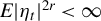
$E | \eta _t |^{2 r} < \infty $
. -
(d)
$\alpha (z) \neq 0 $
for all
$| z | \leqslant 1$
. -
(e) For all
$0 \leq \kappa \leq \lambda $
:
$\operatorname *{\mathrm {plim}}\limits _{T \rightarrow \infty } (1 / \lfloor T \kappa \rfloor ) \sum _{s = 1}^{\lfloor T \kappa \rfloor } g_s g_s'$
is positive definite with finite elements;
$\operatorname *{\mathrm {plim}}\limits _{T \rightarrow \infty } (1 / \lfloor T \kappa \rfloor ) \sum _{s = 1}^{\lfloor T \kappa \rfloor } g_s g_s'/ \sigma _s^2 = \lim \limits _{T \rightarrow \infty } (1 / \lfloor T \kappa \rfloor ) E (\sum _{s = 1}^{\lfloor T \kappa \rfloor } g_s g_s' / \sigma _s^2) =: \Theta (\kappa )$
, where
$\Theta (\kappa )$
is a positive-definite matrix with all elements finite and continuous in
$\kappa $
. Furthermore, we assume that the covariances between
$h_t$
and
$g_t$
and between
$h_t$
and
$g_t g_t'$
are zero, for all
$t=1,\ldots ,T,\dots ,\lfloor \lambda T \rfloor $
. -
(f) The vector
${w}_t$
satisfies
$ \limsup \limits _{T\rightarrow \infty } \frac {1}{\lfloor T\lambda \rfloor } \sum _{t=1}^{\lfloor T\lambda \rfloor } E \|w_t\|^{2+\delta }<\infty $
, for some
$\delta>0$
, where
$\| \cdot \|$
denotes the Euclidean norm.


















Remark 2.3. The monitoring procedure of HB assumes that $v_t$
is homoskedastic, while ATKK allow for conditional heteroskedasticity, but impose unconditional homoskedasticity, in the context of their covariate-augmented PSY and PWY tests. These assumptions are arguably rather strong given that time-varying volatility appears to be a common feature in many financial time series. For example, many empirical studies report strong evidence of structural breaks in the unconditional variance of asset returns (see McMillan and Wohar, Reference McMillan and Wohar2011; Calvo-Gonzalez, Shankar, and Trezzi, Reference Calvo-Gonzalez, Shankar and Trezzi2010; Vivian and Wohar, Reference Vivian and Wohar2012; among others). To allow for such features, Assumption 2(a), which coincides with Assumption 2 of AHLTZ, specifies the unconditional volatility function of the regression errors,
$v_t$
is homoskedastic, while ATKK allow for conditional heteroskedasticity, but impose unconditional homoskedasticity, in the context of their covariate-augmented PSY and PWY tests. These assumptions are arguably rather strong given that time-varying volatility appears to be a common feature in many financial time series. For example, many empirical studies report strong evidence of structural breaks in the unconditional variance of asset returns (see McMillan and Wohar, Reference McMillan and Wohar2011; Calvo-Gonzalez, Shankar, and Trezzi, Reference Calvo-Gonzalez, Shankar and Trezzi2010; Vivian and Wohar, Reference Vivian and Wohar2012; among others). To allow for such features, Assumption 2(a), which coincides with Assumption 2 of AHLTZ, specifies the unconditional volatility function of the regression errors, $\sigma _t$
, to have a flexible nonparametric structure which allows for, inter alia, smooth transition breaks in volatility and trending volatility. The case of constant volatility, where
$\sigma _t$
, to have a flexible nonparametric structure which allows for, inter alia, smooth transition breaks in volatility and trending volatility. The case of constant volatility, where $ \sigma _t = \sigma $
, for all t, also satisfies Assumption 2(a) with
$ \sigma _t = \sigma $
, for all t, also satisfies Assumption 2(a) with $ \sigma (s) = \sigma $
, for all
$ \sigma (s) = \sigma $
, for all $s \in [0 , \lambda ] $
. Although discrete jumps in volatility are not formally allowed under Assumption 2(a), this is not restrictive in practice because one can always approximate discontinuities in
$s \in [0 , \lambda ] $
. Although discrete jumps in volatility are not formally allowed under Assumption 2(a), this is not restrictive in practice because one can always approximate discontinuities in $ \sigma ( \cdot ) $
arbitrarily well using smooth transition functions.Footnote
3
$ \sigma ( \cdot ) $
arbitrarily well using smooth transition functions.Footnote
3
Remark 2.4. Assumption 2(b) specifies that $ \eta _t $
is a conditionally heteroskedastic MDS. Allowing for conditional heteroskedasticity is desirable with financial data and, hence, this represents an important relaxation of the conditions required by AHLTZ who impose conditional homoskedasticity on their equivalent of
$ \eta _t $
is a conditionally heteroskedastic MDS. Allowing for conditional heteroskedasticity is desirable with financial data and, hence, this represents an important relaxation of the conditions required by AHLTZ who impose conditional homoskedasticity on their equivalent of $ \eta _t$
in their Assumption 1. The MDS condition in Assumption 2(b) implies that the exogeneity condition
$ \eta _t$
in their Assumption 1. The MDS condition in Assumption 2(b) implies that the exogeneity condition $E (g_t \eta _t )=0$
holds. Assumption 2(c) additionally imposes that
$E (g_t \eta _t )=0$
holds. Assumption 2(c) additionally imposes that $\eta _t$
is strong mixing. This assumption is made because we need to restrict the amount of dependence in
$\eta _t$
is strong mixing. This assumption is made because we need to restrict the amount of dependence in $\{\eta _t^2-1\}$
(this process no longer being an MDS when conditional heteroskedasticity is present in
$\{\eta _t^2-1\}$
(this process no longer being an MDS when conditional heteroskedasticity is present in $ \eta _t $
) for the purposes of estimating the unconditional volatility function,
$ \eta _t $
) for the purposes of estimating the unconditional volatility function, $ \sigma _t$
(see, e.g., Lemma A.3 in the Supplementary Material). The final condition in Assumption 2(e) rules out any correlation between the regressors in (6),
$ \sigma _t$
(see, e.g., Lemma A.3 in the Supplementary Material). The final condition in Assumption 2(e) rules out any correlation between the regressors in (6), $g_t$
, and the conditional variance of
$g_t$
, and the conditional variance of $\eta _t$
and also rules out correlation between the elements of the design matrix
$\eta _t$
and also rules out correlation between the elements of the design matrix $g_t g_t'$
and the conditional variance of
$g_t g_t'$
and the conditional variance of $\eta _t$
, where
$\eta _t$
, where $ \eta _t$
is conditionally homoskedastic, this condition is rendered redundant. Moreover, this condition is also not needed in the case where an intercept term is not included in (5) (see Section A.1 of the Supplementary Material).
$ \eta _t$
is conditionally homoskedastic, this condition is rendered redundant. Moreover, this condition is also not needed in the case where an intercept term is not included in (5) (see Section A.1 of the Supplementary Material).
Remark 2.5. Assumption 2(d) rules out the presence of unit or explosive autoregressive roots in $\Delta y_t$
under the null hypothesis. Assumption 2(e) allows the covariance matrix of the covariates to display very general patterns of time variation. This condition is weaker than the conditions placed on
$\Delta y_t$
under the null hypothesis. Assumption 2(e) allows the covariance matrix of the covariates to display very general patterns of time variation. This condition is weaker than the conditions placed on $ \sigma _t$
under Assumption 2(a) because any heteroskedasticity arising from the covariates does not show up in the limiting null distribution of the CUSUM statistics that our monitoring procedure is based on and, hence, does not need to be estimated or corrected for. Notice that time variation in the correlation between
$ \sigma _t$
under Assumption 2(a) because any heteroskedasticity arising from the covariates does not show up in the limiting null distribution of the CUSUM statistics that our monitoring procedure is based on and, hence, does not need to be estimated or corrected for. Notice that time variation in the correlation between $ \varepsilon _t$
and the covariates is also permitted.
$ \varepsilon _t$
and the covariates is also permitted.
Remark 2.6. Under Assumptions 2(e) and 2(f), we can make use of the weak convergence result established in Lemma A.10 in the Supplementary Material, which is an extension of Lemma 3 of KPA to our context and plays an important role in the proof of our main results. In Assumption 2(e), the condition that $ \operatorname *{\mathrm {plim}}\limits _{T \rightarrow \infty } (1 / \lfloor T \kappa \rfloor ) \sum _{t = 1}^{\lfloor T \kappa \rfloor } g_t g_t' $
is positive definite with finite elements rules out the possibility of asymptotic collinearity between the regressors in
$ \operatorname *{\mathrm {plim}}\limits _{T \rightarrow \infty } (1 / \lfloor T \kappa \rfloor ) \sum _{t = 1}^{\lfloor T \kappa \rfloor } g_t g_t' $
is positive definite with finite elements rules out the possibility of asymptotic collinearity between the regressors in $ g_t $
. Taken together with the exogeneity condition implied by Assumption 2(b), this ensures least squares (LS) estimation of
$ g_t $
. Taken together with the exogeneity condition implied by Assumption 2(b), this ensures least squares (LS) estimation of $ \varphi $
in Lemma A.1 in the Supplementary Material is consistent under the null hypothesis,
$ \varphi $
in Lemma A.1 in the Supplementary Material is consistent under the null hypothesis, $H_0 : \delta = 0 $
. Likewise, the analogous condition on
$H_0 : \delta = 0 $
. Likewise, the analogous condition on $ \operatorname *{\mathrm {plim}}\limits _{T \rightarrow \infty } (1 / \lfloor T \kappa \rfloor ) \sum _{t = 1}^{\lfloor T \kappa \rfloor } g_t g_t'/\sigma _t^2 $
is required in the context of weighted LS (WLS) estimation of
$ \operatorname *{\mathrm {plim}}\limits _{T \rightarrow \infty } (1 / \lfloor T \kappa \rfloor ) \sum _{t = 1}^{\lfloor T \kappa \rfloor } g_t g_t'/\sigma _t^2 $
is required in the context of weighted LS (WLS) estimation of $ \varphi $
(see Lemma A.6 in the Supplementary Material).
$ \varphi $
(see Lemma A.6 in the Supplementary Material).
Remark 2.7. An analogous moment condition to Assumption 2(f) is imposed for all the covariates (and the error terms) in KPA; notice that we do not need to directly impose this condition on the lagged differences $\Delta y_{t-k}$
,
$\Delta y_{t-k}$
, $ k=1,\ldots ,p$
, in our regression model in (6), because Assumption 2(c) implies that the lagged differences will satisfy an equivalent moment condition, which is stronger than Assumption 2(f). The stronger moment condition in Assumption 2(c) is needed for the proof of Lemma A.3 in the Supplementary Material, which is required in connection with estimation of the (unknown) variance function,
$ k=1,\ldots ,p$
, in our regression model in (6), because Assumption 2(c) implies that the lagged differences will satisfy an equivalent moment condition, which is stronger than Assumption 2(f). The stronger moment condition in Assumption 2(c) is needed for the proof of Lemma A.3 in the Supplementary Material, which is required in connection with estimation of the (unknown) variance function, $ \sigma _t^2$
.
$ \sigma _t^2$
.
Remark 2.8. Our specification for the covariates is more general than is imposed by KPA, who impose a global homoskedasticity assumption, or by Hansen (Reference Hansen1995), Chang, Sickles, and Song (Reference Chang, Sickles and Song2017) [CSS], and ATKK in the context of their covariate unit root testing methods. For example, the (covariance) stationarity assumption required to hold on the covariates by Hansen (Reference Hansen1995) is not imposed by our assumptions as we allow for unconditional heteroskedasticity. Moreover, a version of the unconditionally homoskedastic finite-order stationary vector autoregressive model specified for the covariates in CSS and ATKK, generalized to allow for the possibility of unconditional heteroskedasticity, is also permitted under our assumptions. The assumption made in Hansen (Reference Hansen1995), CSS, and ATKK that the covariates are weakly dependent is not required for our analysis, albeit the strength of dependence allowed is restricted by Assumption 2(e) which, for example, rules out covariates with (near-) unit roots. As argued in Hansen (Reference Hansen1995), in many cases, the first differences of relevant financial and/or macroeconomic time series will be natural covariates to consider.
3 CUSUM-BASED BUBBLE DETECTION PROCEDURES
Under the assumption that $v_{t}$
in (2) is a mean zero, serially uncorrelated and conditionally homoskedastic process with unconditional variance
$v_{t}$
in (2) is a mean zero, serially uncorrelated and conditionally homoskedastic process with unconditional variance $\sigma ^{2}$
, and for a training sample
$\sigma ^{2}$
, and for a training sample $t=1,\ldots ,T $
, as in (1) and (2), HB propose testing for explosive behavior in the monitoring period using the CUSUM statistic:
$t=1,\ldots ,T $
, as in (1) and (2), HB propose testing for explosive behavior in the monitoring period using the CUSUM statistic:
 $$ \begin{align} S_{T}^{t}:=\frac{1}{\tilde{\sigma}_{t}}\sum_{j=T+1}^{t}\Delta y_{j}, \end{align} $$
where $ t> T $
is the monitoring observation. In (7),
$ t> T $
is the monitoring observation. In (7), $\tilde {\sigma }_{t}^{2}$
is an estimate of
$\tilde {\sigma }_{t}^{2}$
is an estimate of $\sigma ^2$
which is consistent under
$\sigma ^2$
which is consistent under $H_{0}$
; HB use
$H_{0}$
; HB use $\tilde {\sigma } _{t}^{2}:=(t-1)^{-1}\sum _{j=2}^{t}\left (\Delta y_{j}\right )^{2}$
. If
$\tilde {\sigma } _{t}^{2}:=(t-1)^{-1}\sum _{j=2}^{t}\left (\Delta y_{j}\right )^{2}$
. If $S_{T}^{t}$
is computed sequentially at dates
$S_{T}^{t}$
is computed sequentially at dates $t=T+1,\dots ,\lfloor \lambda T\rfloor $
, then under the null hypothesis,
$t=T+1,\dots ,\lfloor \lambda T\rfloor $
, then under the null hypothesis, $H_{0}$
, of no explosive behavior, as
$H_{0}$
, of no explosive behavior, as $ T \rightarrow \infty $
,
$ T \rightarrow \infty $
,
 $$ \begin{align} T^{-1/2}S_{T}^{\lfloor Tr\rfloor }\Rightarrow W(r)-W(1),\quad 1<r\leq \lambda, \end{align} $$
where “ $\Rightarrow $
” denotes weak convergence of the associated probability measures, and where
$\Rightarrow $
” denotes weak convergence of the associated probability measures, and where $ W( \cdot ) $
is used generically to denote a standard Brownian motion defined on the interval
$ W( \cdot ) $
is used generically to denote a standard Brownian motion defined on the interval $ [ 0 , \lambda ] $
.
$ [ 0 , \lambda ] $
.
Using Theorem 3.4 of Chu et al. (Reference Chu, Stinchcombe and White1996), HB show that under $H_{0}$
, the result in (8) implies that, for any
$H_{0}$
, the result in (8) implies that, for any $ \lambda> 1 $
,
$ \lambda> 1 $
,
 $$ \begin{align} \lim_{T\rightarrow \infty }\Pr \left( |S_{T}^{t}|>c_{t}\sqrt{t}\,\,\text{for some}\,\,t\in \left\{ T+1,\dots,\lfloor \lambda T\rfloor \right\} \right) \leq \text{exp}\left( -b_{\alpha }/2\right), \end{align} $$
where $c_{t}:=\sqrt {b_{\alpha }+log(t/T)}$
. The CUSUM monitoring procedure proposed in HB then rejects
$c_{t}:=\sqrt {b_{\alpha }+log(t/T)}$
. The CUSUM monitoring procedure proposed in HB then rejects $H_{0}$
if
$H_{0}$
if $S_{T}^{t}>c_{t} \sqrt {t}$
for some
$S_{T}^{t}>c_{t} \sqrt {t}$
for some $t>T$
, with an explosive episode signaled at the first time point t in the monitoring period for which such an exceedance occurs.Footnote
4
For such a (one-sided upper tail) test the appropriate asymptotic setting for
$t>T$
, with an explosive episode signaled at the first time point t in the monitoring period for which such an exceedance occurs.Footnote
4
For such a (one-sided upper tail) test the appropriate asymptotic setting for $b_{\alpha }$
used to compute
$b_{\alpha }$
used to compute $c_t$
that would deliver size of at most
$c_t$
that would deliver size of at most $\alpha =0.05$
would be
$\alpha =0.05$
would be $b_{\alpha }=4.6$
(as this value of
$b_{\alpha }=4.6$
(as this value of $b_{\alpha }$
would deliver a two-sided test with size at most
$b_{\alpha }$
would deliver a two-sided test with size at most $\alpha =0.10$
from the result in (9)).Footnote
5
$\alpha =0.10$
from the result in (9)).Footnote
5
Astill et al. (Reference Astill, Harvey, Leybourne, Sollis and Taylor2018) show that the procedure based on $ S_{T}^{t} $
does not have a controlled FPR, even in large samples, in the case where
$ S_{T}^{t} $
does not have a controlled FPR, even in large samples, in the case where $ v_t = \sigma _t \epsilon _t$
with the volatility function,
$ v_t = \sigma _t \epsilon _t$
with the volatility function, $ \sigma _t$
, displaying time variation of the form specified by Assumption 2(a) and
$ \sigma _t$
, displaying time variation of the form specified by Assumption 2(a) and $\epsilon _t $
an MDS with unit conditional variance. Based on this, AHLTZ replace
$\epsilon _t $
an MDS with unit conditional variance. Based on this, AHLTZ replace $S_{T}^{t}$
with the modified CUSUM statistic
$S_{T}^{t}$
with the modified CUSUM statistic
 $$ \begin{align} SV_{T}^{t}:=\sum_{j=T+1}^{t}\frac{\Delta y_{j}}{\hat{\sigma}_{j,N}} , \; \; t> T, \end{align} $$
where $\hat {\sigma }_{j,N}^{2}$
is a kernel smoothing estimator for the spot variance
$\hat {\sigma }_{j,N}^{2}$
is a kernel smoothing estimator for the spot variance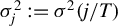 $\sigma _{j}^{2}:=\sigma ^{2}(j/T)$
, defined, for
$\sigma _{j}^{2}:=\sigma ^{2}(j/T)$
, defined, for $ j\geqslant N+1$
, as
$ j\geqslant N+1$
, as
 $$ \begin{align} \hat{\sigma}_{j,N}^{2}:=\sum_{s=0}^{N}k_{s}\left(\Delta y_{j-s}\right)^{2},\quad \mathrm{ with} \quad k_{s}:=\frac{K\left( \frac{s}{N}\right) }{\sum_{s=0}^{N}K\left( \frac{s}{N}\right) }, \end{align} $$
where the kernel function, $K(\cdot )$
, and bandwidth, N, satisfy the conditions stated in Assumption 3, below. AHLTZ establish that the CUSUM monitoring procedure based on
$K(\cdot )$
, and bandwidth, N, satisfy the conditions stated in Assumption 3, below. AHLTZ establish that the CUSUM monitoring procedure based on $SV_{T}^{t}$
is able to control the FPR when
$SV_{T}^{t}$
is able to control the FPR when $v_t$
exhibits time-varying volatility of the form specified in Assumption 2(a), while retaining power close to the standard CUSUM procedure of HB when the innovations are homoskedastic.
$v_t$
exhibits time-varying volatility of the form specified in Assumption 2(a), while retaining power close to the standard CUSUM procedure of HB when the innovations are homoskedastic.
Henceforth, we will refer to a monitoring procedure based on the $S_{T}^{t}$
statistic as the (standard) CUSUM monitoring procedure and that based on the
$S_{T}^{t}$
statistic as the (standard) CUSUM monitoring procedure and that based on the $SV_{T}^{t}$
statistic as the CUSUM
$SV_{T}^{t}$
statistic as the CUSUM $^{V}$
monitoring procedure.
$^{V}$
monitoring procedure.
The validity of both CUSUM and CUSUM $^{V}$
relies on the assumption that
$^{V}$
relies on the assumption that $\Delta y_t$
is serially uncorrelated under
$\Delta y_t$
is serially uncorrelated under $ H_0$
. This assumption is obviously violated if
$ H_0$
. This assumption is obviously violated if $ v_t$
is generated by (4) with
$ v_t$
is generated by (4) with $ p> 0 $
, but is also, in general, violated (even if
$ p> 0 $
, but is also, in general, violated (even if $ p=0 $
) when
$ p=0 $
) when $ \beta (L) \neq {0}$
if, for example, either the covariates,
$ \beta (L) \neq {0}$
if, for example, either the covariates, $ x_t$
, are serially correlated, or
$ x_t$
, are serially correlated, or $ q> 0 $
, or both. The large sample results in (8) and (9) will not hold for
$ q> 0 $
, or both. The large sample results in (8) and (9) will not hold for $S_{T}^{t}$
or
$S_{T}^{t}$
or $SV_{T}^{t}$
in such cases. Consequently implementing CUSUM and CUSUM
$SV_{T}^{t}$
in such cases. Consequently implementing CUSUM and CUSUM $^{V}$
using the critical values from HB would result in monitoring procedures where the (theoretical) FPR would not be at the level expected by the practitioner. We next develop covariate-augmented analogs of the CUSUM and CUSUM
$^{V}$
using the critical values from HB would result in monitoring procedures where the (theoretical) FPR would not be at the level expected by the practitioner. We next develop covariate-augmented analogs of the CUSUM and CUSUM $^{V}$
procedures which account for the influence of the covariates
$^{V}$
procedures which account for the influence of the covariates ${x}_t$
, as well as any serial correlation arising from
${x}_t$
, as well as any serial correlation arising from $\alpha (L)$
. These will be shown to retain the large sample results in (8) and (9). Later, in Section 5, we will use Monte Carlo simulation to investigate the degree of spurious detections suffered by the univariate procedures when covariates are present in the DGP, and show that these are well controlled by the covariate-augmented procedures.
$\alpha (L)$
. These will be shown to retain the large sample results in (8) and (9). Later, in Section 5, we will use Monte Carlo simulation to investigate the degree of spurious detections suffered by the univariate procedures when covariates are present in the DGP, and show that these are well controlled by the covariate-augmented procedures.
4 A COVARIATE-AUGMENTED CUSUM MONITORING PROCEDURE
CUSUM tests for structural change in the parameters of homoskedastic weakly dependent dynamic regression models have been developed in KPA who base their approach on a statistic constructed from a standardized cumulated sum of recursive LS residuals. We will adapt this approach to our setting to develop a real-time bubble monitoring procedure which has a theoretically controlled FPR when $ v_t$
is generated according to (4). We discuss the construction of the CUSUM monitoring statistic by first considering the infeasible case where the volatility function,
$ v_t$
is generated according to (4). We discuss the construction of the CUSUM monitoring statistic by first considering the infeasible case where the volatility function, $\sigma _t$
, is known, and then discuss the feasible version of this, based on nonparametric estimation of
$\sigma _t$
, is known, and then discuss the feasible version of this, based on nonparametric estimation of $ \sigma _t$
.
$ \sigma _t$
.
A key difference between our setting and that considered in KPA is that we allow for the presence of heteroskedasticity in both the covariates, $x_t$
, and in disturbances,
$x_t$
, and in disturbances, $\varepsilon _t$
, in the null regression (5), of the form specified in Assumption 2. Except in the special case where the intercept term is excluded from the null regression (recall that this may be done where the covariates all have mean zero), which is discussed separately in Section A.1 of the Supplementary Material, the presence of unconditional heteroskedasticity necessitates constructing the CUSUM monitoring statistics from recursive WLS residuals, rather than the conventional recursive LS residuals which suffice under unconditional homoskedasticity. It is also worth clarifying at this point that the methods outlined in this section apply provided that the vector of regression variables,
$\varepsilon _t$
, in the null regression (5), of the form specified in Assumption 2. Except in the special case where the intercept term is excluded from the null regression (recall that this may be done where the covariates all have mean zero), which is discussed separately in Section A.1 of the Supplementary Material, the presence of unconditional heteroskedasticity necessitates constructing the CUSUM monitoring statistics from recursive WLS residuals, rather than the conventional recursive LS residuals which suffice under unconditional homoskedasticity. It is also worth clarifying at this point that the methods outlined in this section apply provided that the vector of regression variables, $g_t$
, in the null regression model, (6), contains at least one element (even if this is just an intercept term). Where this is not the case, no regression estimation is needed and the appropriate monitoring procedure is that given in Section 2.2 of AHLTZ.
$g_t$
, in the null regression model, (6), contains at least one element (even if this is just an intercept term). Where this is not the case, no regression estimation is needed and the appropriate monitoring procedure is that given in Section 2.2 of AHLTZ.
Our proposed CUSUM monitoring statistic is based on recursive WLS estimation of the (null) regression in (6), which contains $1 + p + (q+1) m$
regressors. To that end, consider the infeasible WLS transformation of (6), based on the true volatility function
$1 + p + (q+1) m$
regressors. To that end, consider the infeasible WLS transformation of (6), based on the true volatility function $ \sigma _t$
, given by
$ \sigma _t$
, given by
 $$ \begin{align} \frac{\Delta y_t}{\sigma_t} = \varphi' \frac{g_t}{\sigma_t} + \eta_t, \quad t = 1, \ldots, T, \dots, \lfloor \lambda T \rfloor. \end{align} $$
The (infeasible) WLS estimator for $\varphi $
at time t in the monitoring sample from this regression is then given by
$\varphi $
at time t in the monitoring sample from this regression is then given by
 $$\begin{align*}{\varphi}_t^W := \left( \sum_{j = \text{max}(p+2,q+1)}^t \frac{g_j g_j' }{\sigma_j^2} \right)^{- 1} \left( \sum_{j = \text{max}(p+2,q+1)}^t \frac{g_j \Delta y_j}{\sigma_j^2} \right), \quad t = T + 1, \dots, \lfloor \lambda T \rfloor \end{align*}$$
with the associated (infeasible) recursive residuals based on the WLS estimate defined as
 $$ \begin{align} e^{W}_t := {\Delta y_t} - ({\varphi}_{t - 1}^{W})' g_t, \quad t = T + 1, \dots, \lfloor \lambda T \rfloor. \end{align} $$
It is established in the proof of Theorem 1 that, under the null hypothesis, the associated infeasible sequence of CUSUM statistics $ SWM_{T}^{t} := \sum _{j = T + 1}^{t} {e_j^{W}}/{\sigma _j} $
,
$ SWM_{T}^{t} := \sum _{j = T + 1}^{t} {e_j^{W}}/{\sigma _j} $
, $ t = T+ 1,\dots , \lfloor \lambda T \rfloor $
, satisfies
$ t = T+ 1,\dots , \lfloor \lambda T \rfloor $
, satisfies $ T^{-1/2} SWM^{\lfloor T r \rfloor }_T \Rightarrow {W} (r) - {W} (1) $
,
$ T^{-1/2} SWM^{\lfloor T r \rfloor }_T \Rightarrow {W} (r) - {W} (1) $
, $ 1 < r \leq \lambda $
, where it is recalled that
$ 1 < r \leq \lambda $
, where it is recalled that ${W} ( \cdot ) $
generically denotes a standard Brownian motion on
${W} ( \cdot ) $
generically denotes a standard Brownian motion on $ [ 0, \lambda ] $
, such that we recover the usual limiting distribution in (8).
$ [ 0, \lambda ] $
, such that we recover the usual limiting distribution in (8).
To obtain a feasible version of $SWM_{T}^{t}$
, we need to replace
$SWM_{T}^{t}$
, we need to replace $\sigma _j$
by a nonparametric estimate thereof. Nonparametric estimation of the variance function in time-series models has been considered by, among others, Xu and Phillips (Reference Xu and Phillips2008), Cavaliere et al. (Reference Cavaliere, Nielsen and Taylor2022), and Harvey et al. (Reference Harvey, Leybourne and Zu2019), whereby a nonparametric kernel smoothing estimation procedure is applied to the squares of regression residuals from the model at hand. In the present real-time monitoring setting, however, nonparametric estimation of the variance function is nonstandard in two ways. First, because the monitoring takes place in real time, only data up to and including each time point in the monitoring period will be available to the practitioner, and so as a consequence, the smoothing is naturally performed using a one-sided kernel. Second, because new data will continue to arrive in real time as the monitoring proceeds, the vector of regression residuals needs to be updated at each successive time point in the monitoring period.
$\sigma _j$
by a nonparametric estimate thereof. Nonparametric estimation of the variance function in time-series models has been considered by, among others, Xu and Phillips (Reference Xu and Phillips2008), Cavaliere et al. (Reference Cavaliere, Nielsen and Taylor2022), and Harvey et al. (Reference Harvey, Leybourne and Zu2019), whereby a nonparametric kernel smoothing estimation procedure is applied to the squares of regression residuals from the model at hand. In the present real-time monitoring setting, however, nonparametric estimation of the variance function is nonstandard in two ways. First, because the monitoring takes place in real time, only data up to and including each time point in the monitoring period will be available to the practitioner, and so as a consequence, the smoothing is naturally performed using a one-sided kernel. Second, because new data will continue to arrive in real time as the monitoring proceeds, the vector of regression residuals needs to be updated at each successive time point in the monitoring period.
As a consequence of the second issue discussed above, we will need to make use of the double array of ordinary LS (OLS) residuals from estimating (5), defined as
 $$ \begin{align} f_{i, t}^* := \Delta y_i - (\hat{\varphi}_t)' g_i, \quad i = \text{max}(p+2,q+1), \dots, t, \; t = T + 1, \dots, \lfloor \lambda T \rfloor, \end{align} $$
where
 $$ \begin{align} \hat{\varphi}_t := \left( \sum_{j = \text{max}(p+2,q+1)}^t {g}_j {g}_j' \right)^{- 1} \left( \sum_{j = \text{max}(p+2,q+1)}^t {g}_j \Delta y_j \right), \quad t = T + 1, \dots, \lfloor \lambda T \rfloor. \end{align} $$
Using the OLS residuals in (14), we can then define the sequence of nonparametric variance estimators across times $ j = N+\text {max}(p+1,q),\ldots ,t $
, when standing at time t, as
$ j = N+\text {max}(p+1,q),\ldots ,t $
, when standing at time t, as
 $$ \begin{align} \tilde{\sigma}_{j,N,t}^{2}:= \sum_{s = 0}^N k_s ( f_{j - s, t}^* )^2, \quad k_s := \frac{K \left( \frac{s}{N} \right)}{\sum_{s = 0}^N K \left( \frac{s}{N} \right)}, \end{align} $$
in which $k_s$
,
$k_s$
, $s=0,\ldots ,N$
, is a sequence of weights, which are defined based on some kernel function
$s=0,\ldots ,N$
, is a sequence of weights, which are defined based on some kernel function $K ( \cdot )$
and a window size N, precise conditions on which will be given in Assumption 3, below. Because of the unavailability of future data, this nonparametric variance estimator uses a left-sided, truncated kernel. Only the N most recent observations are used in the calculation of the estimator and the weights are not dependent on t.
$K ( \cdot )$
and a window size N, precise conditions on which will be given in Assumption 3, below. Because of the unavailability of future data, this nonparametric variance estimator uses a left-sided, truncated kernel. Only the N most recent observations are used in the calculation of the estimator and the weights are not dependent on t.
Based on the nonparametric variance estimates in (16), we can then define the feasible WLS estimator of $ \varphi $
at time t asFootnote
6
$ \varphi $
at time t asFootnote
6
 $$\begin{align*}\hat{\varphi}_{t}^{W} := \left( \sum_{j = N+\text{max}(p+1,q)}^{t} \frac{g_j g_j'}{\tilde{\sigma}_{j,N,t}^2} \right)^{- 1} \left( \sum_{j = N+\text{max}(p+1,q)}^{t} \frac{g_j \Delta y_j}{\tilde{\sigma}_{j,N,t}^2} \right), \quad t = T + 1, \dots, \lfloor \lambda T \rfloor. \end{align*}$$
Defining the feasible WLS recursive residuals as
 $$ \begin{align*}{\hat{e}_j^{W}}:=\Delta y_j - (\hat{\varphi}_{j - 1}^{W})' g_j , \quad j = T + 1, \dots, \lfloor \lambda T \rfloor \end{align*} $$
a feasible version of the sequence of $SWM_{T}^{t}$
statistics can then defined as
$SWM_{T}^{t}$
statistics can then defined as
 $$ \begin{align} SWMV^{ t }_T := \sum_{j = T + 1}^{ t } \frac{\hat{e}_j^{W}}{\tilde{\sigma}_{j,N,j}} , \qquad t = T+1,\dots, \lfloor \lambda T \rfloor. \end{align} $$
We will denote the monitoring procedure based on the sequence of $SWMV^{t}_T$
,
$SWMV^{t}_T$
, $ t = T+1 ,\dots , \lfloor \lambda T \rfloor $
, statistics as CUSUM
$ t = T+1 ,\dots , \lfloor \lambda T \rfloor $
, statistics as CUSUM $^{WMV}$
.
$^{WMV}$
.
In order to derive the asymptotic properties of the sequence of $SWMV_{T}^{t}$
statistics, we require the following conditions hold on the kernel function
$SWMV_{T}^{t}$
statistics, we require the following conditions hold on the kernel function $K (\cdot )$
and the window size N. These conditions coincide with those imposed by AHLTZ (p. 194) in the context of their
$K (\cdot )$
and the window size N. These conditions coincide with those imposed by AHLTZ (p. 194) in the context of their $ SV_{T}^{t} $
statistic in (10), where a discussion of these conditions is provided.
$ SV_{T}^{t} $
statistic in (10), where a discussion of these conditions is provided.
Assumption 3.
-
(a)
$K ( \cdot )$
is strictly positive and continuously differentiable over the interval
$(0, 1)$
, with
$K (x) = 0$
for
$x \leq 0$
and
$x \geq 1$
. Also,
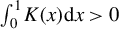
$\int _0^1 K (x) \mathrm {d} x> 0$
,
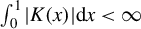
$\int _0^1 |K (x) | \mathrm {d} x < \infty $
,
$\int _0^1 |K (x) x| \mathrm {d} x < \infty $
and the characteristic function
$\phi (t) = \int _{- \infty }^{\infty } \exp (\mathrm {i} tx) K (x) \mathrm {d} x$
of K satisfies
$\int _{- \infty }^{\infty } | \phi (t) | \mathrm {d} t < \infty $
.
$K' (\cdot )$
, the derivative of the
$K ( \cdot )$
function, also has a characteristic function that is absolutely integrable. -
(b)
$N \rightarrow \infty $
as
$T \rightarrow \infty $
, such that
$N / T \rightarrow 0$
and
$N^{3 / 2} / T \rightarrow \infty $
.








Remark 4.1. Implementation of $SWMV_{T}^{t}$
requires choices to be made for both the kernel and bandwidth used in constructing the nonparametric estimator
$SWMV_{T}^{t}$
requires choices to be made for both the kernel and bandwidth used in constructing the nonparametric estimator $\tilde {\sigma }_{j,N,t}^{2}$
in (16). We found that the choices for these recommended in AHLTZ also lead to good FPR control for the procedures considered in this article. Specifically, we therefore recommend implementation with the truncated Gaussian kernel and where the bandwidth at each point t in the monitoring period, denoted
$\tilde {\sigma }_{j,N,t}^{2}$
in (16). We found that the choices for these recommended in AHLTZ also lead to good FPR control for the procedures considered in this article. Specifically, we therefore recommend implementation with the truncated Gaussian kernel and where the bandwidth at each point t in the monitoring period, denoted $N_t^{cv}$
, is chosen according to the automated rule:
$N_t^{cv}$
, is chosen according to the automated rule:
 $$ \begin{align} N_t^{cv *}:= \text{argmin}_{N \in[1,H]}CV^*_t(N), \qquad CV^*_t(N):=\frac{1}{H}\sum_{j=t-H+1}^{t}(\tilde{\sigma}_{j,N,t}^{2} -(f_{j,t}^{*})^2)^{2}, \end{align} $$
where, for $ j = t-H+1,\ldots ,t$
,
$ j = t-H+1,\ldots ,t$
,
 $$ \begin{align} \tilde{\sigma}_{j,N,t}^{2}:= \sum_{s = 0}^N k_s (f_{j - s, t}^*)^2, \quad k_s := \frac{K \left( \frac{s}{N} \right)}{\sum_{s = 0}^N K \left( \frac{s}{N} \right)}. \end{align} $$
The estimators of the spot variances, $ \sigma _j^2 $
,
$ \sigma _j^2 $
, $ j = t-H+1,\ldots ,t$
, each computed at time t, defined in (19) are needed to compute the time t cross-validation objective function in (18). The automated bandwidth rule minimizes the estimation error of the spot variance over the most recent H observations based on the OLS residuals computed using data up to and including the current monitoring observation, t (cf. Hall and Schucany, Reference Hall and Schucany1989). Implementation of
$ j = t-H+1,\ldots ,t$
, each computed at time t, defined in (19) are needed to compute the time t cross-validation objective function in (18). The automated bandwidth rule minimizes the estimation error of the spot variance over the most recent H observations based on the OLS residuals computed using data up to and including the current monitoring observation, t (cf. Hall and Schucany, Reference Hall and Schucany1989). Implementation of $N_t^{cv *} $
in (18) requires a choice of H; we follow AHLTZ and set
$N_t^{cv *} $
in (18) requires a choice of H; we follow AHLTZ and set $H=20$
. These choices for the kernel and bandwidth are used in all the numerical work in this article.
$H=20$
. These choices for the kernel and bandwidth are used in all the numerical work in this article.
In Theorem 1, we establish the joint limiting null distribution of the sequence of feasible covariate-augmented $ SWMV_{T}^{t} $
statistics from the monitoring period.
$ SWMV_{T}^{t} $
statistics from the monitoring period.
Theorem 1. Let the data be generated according to (1)–(4) under the null hypothesis $H_0 : \delta =0 $
. If Assumptions 1–3 hold, then, as
$H_0 : \delta =0 $
. If Assumptions 1–3 hold, then, as $T \rightarrow \infty $
, it follows that
$T \rightarrow \infty $
, it follows that
 $$ \begin{align} T^{-1/2} SWMV^{\lfloor T r \rfloor}_T \Rightarrow {W} (r) - {W} (1), \quad 1 < r \leq \lambda. \end{align} $$
Appealing to Theorem 3.4 of Chu et al. (Reference Chu, Stinchcombe and White1996), Theorem 1 implies the following.
Corollary 1. Under the conditions of Theorem 1,
 $$ \begin{align} \lim_{T \rightarrow \infty} \Pr \left( | SWMV_{T}^{t} |> c_t\sqrt{t} \hspace{0.17em} \hspace{0.17em} \text{for some} \hspace{0.17em} \hspace{0.17em} t \in \{ T + 1,\dots, \lfloor \lambda T \rfloor \} \right) \leq \exp (- b_{\alpha} / 2). \end{align} $$
Remark 4.2. Theorem 1 and Corollary 1 imply that when the innovations $v_t$
satisfy Assumptions 1 and 2, both the limiting null distribution and crossing probabilities for the covariate-augmented CUSUM
$v_t$
satisfy Assumptions 1 and 2, both the limiting null distribution and crossing probabilities for the covariate-augmented CUSUM $^{WMV}$
procedure are unchanged relative to those given in (8) and (9), respectively, for the original CUSUM procedure of HB in the case, where
$^{WMV}$
procedure are unchanged relative to those given in (8) and (9), respectively, for the original CUSUM procedure of HB in the case, where $ v_t$
is conditionally homoskedastic and serially uncorrelated. Notice from (20) that the joint limiting null distribution of the
$ v_t$
is conditionally homoskedastic and serially uncorrelated. Notice from (20) that the joint limiting null distribution of the $SWMV_{T}^{t}$
,
$SWMV_{T}^{t}$
, $ t> T $
, statistics does not depend on any nuisance parameters arising from time-varying behavior in the unconditional covariance matrix of the covariates (cf. Remark 2.5).
$ t> T $
, statistics does not depend on any nuisance parameters arising from time-varying behavior in the unconditional covariance matrix of the covariates (cf. Remark 2.5).
Next, we proceed to establish consistency results for our covariate-augmented CUSUM $^{WMV}$
monitoring procedure. In Theorem 2, we establish consistency results for a class of mildly explosive alternatives of the form
$^{WMV}$
monitoring procedure. In Theorem 2, we establish consistency results for a class of mildly explosive alternatives of the form $\delta = c/T^d $
with
$\delta = c/T^d $
with $0< d \leq 2/3 $
, for
$0< d \leq 2/3 $
, for $ t> \lfloor \tau T \rfloor $
, where c is a positive constant, and for fixed alternatives,
$ t> \lfloor \tau T \rfloor $
, where c is a positive constant, and for fixed alternatives, $ \delta = c $
. We will subsequently discuss the class of mildly explosive alternatives, where
$ \delta = c $
. We will subsequently discuss the class of mildly explosive alternatives, where $ 2/3 < d < 1 $
in Remark 4.3, and locally explosive alternatives, where
$ 2/3 < d < 1 $
in Remark 4.3, and locally explosive alternatives, where $ d=1 $
, in Remark 4.4.
$ d=1 $
, in Remark 4.4.
Theorem 2. Let the data be generated according to (1)–(4) under the alternative hypothesis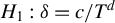 $H_1 : \delta = c/T^d $
, for
$H_1 : \delta = c/T^d $
, for $ t> \lfloor \tau T \rfloor $
, with c a positive constant and
$ t> \lfloor \tau T \rfloor $
, with c a positive constant and $0\leq d \leq 2/3$
, and let Assumptions 1–3 hold. It then holds that
$0\leq d \leq 2/3$
, and let Assumptions 1–3 hold. It then holds that
 $$ \begin{align} \lim_{T \rightarrow \infty} \Pr \left( | SWMV_{T}^{t} |> c_t \sqrt{t}, \text{for some} \hspace{0.30em} t \in \{\lfloor \tau T\rfloor + 1, \dots, \lfloor \lambda T \rfloor\} \right) = 1. \end{align} $$
Remark 4.3. The result in Theorem 2 immediately implies that the CUSUM $^{WMV}$
procedure is consistent against both fixed (
$^{WMV}$
procedure is consistent against both fixed ( $d = 0$
) and mildly explosive (
$d = 0$
) and mildly explosive ( $0 < d \leq 2/3 $
) alternatives of the form
$0 < d \leq 2/3 $
) alternatives of the form $ \delta = c /T^d $
. In both these cases, T
d
maintains a fixed relative relationship with N. Recall that Assumption 3
b imposes the condition that N
3/2/T →∞, which implies that
$ \delta = c /T^d $
. In both these cases, T
d
maintains a fixed relative relationship with N. Recall that Assumption 3
b imposes the condition that N
3/2/T →∞, which implies that ${N}/{T^{2/3}}\rightarrow \infty $
. Consequently, when
${N}/{T^{2/3}}\rightarrow \infty $
. Consequently, when $0\leq d \leq 2/3$
, T
d
diverges at a slower rate than N and
$0\leq d \leq 2/3$
, T
d
diverges at a slower rate than N and $T^d \wedge N = T^d$
. However, in cases where
$T^d \wedge N = T^d$
. However, in cases where $ 2/3 < d < 1 $
, such that the magnitude of the explosiveness parameter is very mild, this no longer holds and, as a result,
$ 2/3 < d < 1 $
, such that the magnitude of the explosiveness parameter is very mild, this no longer holds and, as a result, $ SWMV_{T}^{t} $
does not necessarily diverge at a faster rate than the boundary function c
t
t. Essentially, this issue arises because the volatility estimates in (16) are constructed using the residuals from a regression model which imposes the null hypothesis. Where the null is false, this model is misspecified, and for
$ SWMV_{T}^{t} $
does not necessarily diverge at a faster rate than the boundary function c
t
t. Essentially, this issue arises because the volatility estimates in (16) are constructed using the residuals from a regression model which imposes the null hypothesis. Where the null is false, this model is misspecified, and for $ 2/3 < d < 1 $
, the volatility estimate diverges at such a rate that it prevents CUSUM
$ 2/3 < d < 1 $
, the volatility estimate diverges at such a rate that it prevents CUSUM $^{WMV}$
from necessarily diverging at a faster rate than the boundary function c
t
t (see Lemma A.9 in the Supplementary Material). A possible solution to this is to employ a truncated volatility estimator of the form,
$^{WMV}$
from necessarily diverging at a faster rate than the boundary function c
t
t (see Lemma A.9 in the Supplementary Material). A possible solution to this is to employ a truncated volatility estimator of the form, $\tilde {\sigma }_{j, N, j} \cdot \mathbb {I}(\tilde {\sigma }_{j, N, j} \leq \mathbb {C}\ln (T))+\mathbb {C} \ln (T) \cdot \mathbb {I}(\tilde {\sigma }_{j, N, j}> \mathbb {C} \ln (T))$
, where
$\tilde {\sigma }_{j, N, j} \cdot \mathbb {I}(\tilde {\sigma }_{j, N, j} \leq \mathbb {C}\ln (T))+\mathbb {C} \ln (T) \cdot \mathbb {I}(\tilde {\sigma }_{j, N, j}> \mathbb {C} \ln (T))$
, where $\mathbb {C}$
is a generic positive constant, such that
$\mathbb {C}$
is a generic positive constant, such that $\mathbb {C} \ln (T)$
serves as a slowly varying truncation function. Under the null, the volatility estimator is consistent and the truncation level
$\mathbb {C} \ln (T)$
serves as a slowly varying truncation function. Under the null, the volatility estimator is consistent and the truncation level $\ln (T)$
approaches infinity, such that the truncation has no impact in the limit. However, under the alternative, the truncated volatility estimator is limited to diverge at a rate no faster than
$\ln (T)$
approaches infinity, such that the truncation has no impact in the limit. However, under the alternative, the truncated volatility estimator is limited to diverge at a rate no faster than $\ln (T)$
, which is slower than any polynomial rate. By incorporating this truncation mechanism, we conjecture that consistency would hold over a wider range of d than
$\ln (T)$
, which is slower than any polynomial rate. By incorporating this truncation mechanism, we conjecture that consistency would hold over a wider range of d than $0 \leq d \leq 2/3$
. However, we leave a detailed treatment of this case for future research.
$0 \leq d \leq 2/3$
. However, we leave a detailed treatment of this case for future research.
Remark 4.4. In addition to the consistency results in Theorem 2, it is also instructive to examine the behavior of the monitoring procedure in the case of locally explosive alternatives of the form $ H_{c,\tau }:\delta = c / T$
, for
$ H_{c,\tau }:\delta = c / T$
, for $ t> \lfloor \tau T \rfloor $
, where c is a positive constant. When the volatility process is known, the asymptotic behavior of the detector
$ t> \lfloor \tau T \rfloor $
, where c is a positive constant. When the volatility process is known, the asymptotic behavior of the detector $ {SWMV}_T^t$
can be derived along the same line of argument as the proof of Theorem 1. In particular, in the special case of
$ {SWMV}_T^t$
can be derived along the same line of argument as the proof of Theorem 1. In particular, in the special case of $\alpha (L) = 1$
(i.e., when the fitted model has no lagged dependent variables),
$\alpha (L) = 1$
(i.e., when the fitted model has no lagged dependent variables),
 $$\begin{align*}\frac{1}{\sqrt{T}} \sum_{j = T + 1}^{\lfloor Tr \rfloor} \frac{e_j^W}{\sigma_j} = \frac{1}{\sqrt{T}} \sum_{j = T + 1}^{\lfloor Tr \rfloor} \eta_j - \frac{1}{\sqrt{T}} \sum_{j = T + 1}^{\lfloor Tr \rfloor} \frac{(\varphi^W_{j - 1} - \varphi)' g_j}{\sigma_j} + \frac{c}{T^{3 / 2}} \sum_{j = \lfloor \tau T \rfloor + 1}^{\lfloor Tr \rfloor} \frac{u_{j - 1}}{\sigma_j}. \end{align*}$$
As in the proof of Theorem 1, the first two terms collectively weakly converge to $W (r) - W (1)$
. By the FCLT and CMT, the third term satisfies
$W (r) - W (1)$
. By the FCLT and CMT, the third term satisfies $\frac {c}{T^{3 / 2}} \sum _{j = \lfloor \tau T \rfloor + 1}^{\lfloor Tr \rfloor } \frac {u_{j - 1}}{\sigma _j} \Rightarrow c \int _{\tau }^r U (s) / \sigma (s) {\mathrm {d}} s$
, where
$\frac {c}{T^{3 / 2}} \sum _{j = \lfloor \tau T \rfloor + 1}^{\lfloor Tr \rfloor } \frac {u_{j - 1}}{\sigma _j} \Rightarrow c \int _{\tau }^r U (s) / \sigma (s) {\mathrm {d}} s$
, where $U (s) := \int _0^s e^{c (s - u)} \sigma (u) {\mathrm {d}} W (u)$
. It therefore follows that the asymptotic distribution under
$U (s) := \int _0^s e^{c (s - u)} \sigma (u) {\mathrm {d}} W (u)$
. It therefore follows that the asymptotic distribution under $H_{c, \tau }$
is given by
$H_{c, \tau }$
is given by $W (r) - W (1) + c \int _{\tau }^r U (s) / \sigma (s) {\mathrm {d}} s$
, from which the asymptotic probability of the CUSUM
$W (r) - W (1) + c \int _{\tau }^r U (s) / \sigma (s) {\mathrm {d}} s$
, from which the asymptotic probability of the CUSUM $^{WMV}$
procedure rejecting the null when a locally explosive episode is present can be simulated. For general
$^{WMV}$
procedure rejecting the null when a locally explosive episode is present can be simulated. For general $\alpha (L)$
, it can be shown in the same way that the asymptotic distribution is given by
$\alpha (L)$
, it can be shown in the same way that the asymptotic distribution is given by $W (r) - W (1) + \alpha (1) c \int _{\tau }^r U (s) / \sigma (s) {\mathrm {d}} s$
. Where the volatility is estimated, we anticipate the same limit will hold under
$W (r) - W (1) + \alpha (1) c \int _{\tau }^r U (s) / \sigma (s) {\mathrm {d}} s$
. Where the volatility is estimated, we anticipate the same limit will hold under $H_{c, \tau }$
in view of the results given in Harvey et al. (Reference Harvey, Leybourne and Zu2019) for the behavior of the nonparametric variance estimator considered in this article under locally explosive DGPs.
$H_{c, \tau }$
in view of the results given in Harvey et al. (Reference Harvey, Leybourne and Zu2019) for the behavior of the nonparametric variance estimator considered in this article under locally explosive DGPs.
Remark 4.5. Thus far, we have assumed that the parameters p and q in (5), together with the composition of the m-vector of true covariates, $ x_{t} $
, are known. In practice, these aspects will be unknown. However, under the maintained hypothesis of no bubble in the training sample, the regression model in (5), for
$ x_{t} $
, are known. In practice, these aspects will be unknown. However, under the maintained hypothesis of no bubble in the training sample, the regression model in (5), for $ t=1,\ldots ,T $
, is an
$ t=1,\ldots ,T $
, is an $ARX$
model satisfying standard regularity conditions, and so an application of a consistent information criterion (IC), such as the well-known Bayesian IC (BIC), could be used to select these elements. The Monte Carlo results in Section 5 will implement applying the BIC to the training sample to select p, q, and whether to include a given candidate covariate or not.
$ARX$
model satisfying standard regularity conditions, and so an application of a consistent information criterion (IC), such as the well-known Bayesian IC (BIC), could be used to select these elements. The Monte Carlo results in Section 5 will implement applying the BIC to the training sample to select p, q, and whether to include a given candidate covariate or not.
We end this section with a word of caution. The CUSUM $^{WMV}$
procedure can, in principle, reject for various forms of structural change in the null model that, while ruled by our regularity conditions, might occur in practice. As such, a rejection by CUSUM
$^{WMV}$
procedure can, in principle, reject for various forms of structural change in the null model that, while ruled by our regularity conditions, might occur in practice. As such, a rejection by CUSUM $^{WMV}$
does not necessarily imply the presence of a bubble episode. Indeed, this is precisely our motivation for developing a procedure robust to structural changes in unconditional volatility. Another possibility is where a covariate used in the null regression displays structural change, such as an explosive episode itself or a mean shift; simulations looking at these cases are reported in Section 5.3. In practice, as with any statistical procedure, we recommend practitioners investigate the plausibility of the regularity conditions underlying CUSUM
$^{WMV}$
does not necessarily imply the presence of a bubble episode. Indeed, this is precisely our motivation for developing a procedure robust to structural changes in unconditional volatility. Another possibility is where a covariate used in the null regression displays structural change, such as an explosive episode itself or a mean shift; simulations looking at these cases are reported in Section 5.3. In practice, as with any statistical procedure, we recommend practitioners investigate the plausibility of the regularity conditions underlying CUSUM $^{WMV}$
as part of their statistical analysis. This could, for example, include running standard tests for explosivity and mean shifts in the covariates over the training sample and then running analogous (univariate) CUSUM monitoring procedures in tandem on the covariates, removing any covariate from the analysis for which either of these reject.
$^{WMV}$
as part of their statistical analysis. This could, for example, include running standard tests for explosivity and mean shifts in the covariates over the training sample and then running analogous (univariate) CUSUM monitoring procedures in tandem on the covariates, removing any covariate from the analysis for which either of these reject.
5 MONTE CARLO SIMULATIONS
We report results of a Monte Carlo simulation exercise evaluating the finite sample performance of the CUSUM $^{WMV}$
monitoring procedure. Additional results are reported in the Supplementary Material and summarized in Section 5.3.
$^{WMV}$
monitoring procedure. Additional results are reported in the Supplementary Material and summarized in Section 5.3.
5.1 Simulation DGP and Experimental Settings
Data were generated according to (1) and (2), initialized at $u_{0}=100$
(so that bubbles in our series are generally upwardly explosive and, hence, empirically relevant), setting
$u_{0}=100$
(so that bubbles in our series are generally upwardly explosive and, hence, empirically relevant), setting $\mu =0$
without loss of generality. We set
$\mu =0$
without loss of generality. We set $T=219$
, so that monitoring begins at time
$T=219$
, so that monitoring begins at time $t=220$
, and set monitoring to end at time
$t=220$
, and set monitoring to end at time $\lambda T =255$
. Under the null
$\lambda T =255$
. Under the null $\delta =0$
, while under the alternative we set
$\delta =0$
, while under the alternative we set $\delta =0.005$
,
$\delta =0.005$
, $ \tau _1 T = 220$
, and
$ \tau _1 T = 220$
, and $ \tau _2 T = \lambda T$
, such that
$ \tau _2 T = \lambda T$
, such that $y_t$
follows a unit root process during the training sample, before switching to an explosive regime starting when monitoring commences and continuing until the end of the monitoring period.
$y_t$
follows a unit root process during the training sample, before switching to an explosive regime starting when monitoring commences and continuing until the end of the monitoring period.
For the error term $ v_t $
and the covariate
$ v_t $
and the covariate $ x_t $
, we use an unconditionally heteroskedastic extension of the simulation DGP detailed in Section 5.1 on page 143 of CSS:
$ x_t $
, we use an unconditionally heteroskedastic extension of the simulation DGP detailed in Section 5.1 on page 143 of CSS:
 $$ \begin{align} v_t &= \alpha_{1} v_{t-1} + \beta x_{t} + \varepsilon_{1,t}, \end{align} $$
 $$ \begin{align} x_{t+1} &= \rho x_{t} + \varepsilon_{2,t}\end{align} $$
-->with the covariate initialized at $ x_0 = 0 $
. The variance matrix of the innovation vector,
$ x_0 = 0 $
. The variance matrix of the innovation vector, $ ( \varepsilon _{1,t} , \varepsilon _{2,t} )^\prime $
, was generated according to
$ ( \varepsilon _{1,t} , \varepsilon _{2,t} )^\prime $
, was generated according to
 $$ \begin{align} \left(\begin{array}{c} \varepsilon_{1,t} \\ \varepsilon_{2,t} \end{array} \right) \sim NIID ( 0 , \Sigma_t ), \qquad \Sigma_t := \left[\begin{array}{cc} \sigma_{1,t}^2 & \sigma_{12,t} \\ \sigma_{12,t} & \sigma_{2,t}^2 \end{array}\right] \end{align} $$
in which $\sigma _{1,t}^2$
and
$\sigma _{1,t}^2$
and $\sigma _{2,t}^2$
are subject to smooth upward shifts in volatility of the form:
$\sigma _{2,t}^2$
are subject to smooth upward shifts in volatility of the form:
 $$ \begin{align} \sigma _{j,t} &:= 1+(\sqrt{4}-1)\left[ 1+\exp (-\theta (t-219) ) \right]^{-1} , \qquad j= 1,2 \end{align} $$
with $\theta =0.25$
; that is, a logistic smooth transition in volatility from 1 to
$\theta =0.25$
; that is, a logistic smooth transition in volatility from 1 to $\sqrt {4}$
centered on the end of the training sample. We report results for the following four cases for
$\sqrt {4}$
centered on the end of the training sample. We report results for the following four cases for $ \Sigma _t $
:
$ \Sigma _t $
:
-
(a)
$ \sigma _{1,t}^2 = \sigma _{2,t}^2 = 1 $
and
$ \sigma _{12,t} = \sigma _{12}$
, in each case for all t, such that
$\varepsilon _{1,t}$
and
$\varepsilon _{2,t}$
are homoskedastic with a fixed correlation of
$\sigma _{12}$
. -
(b)
$\sigma _{1,t}$
and
$\sigma _{2,t}$
both satisfy (26), while
$ \sigma _{12,t} = \sigma _{12} \sigma _{1,t} \sigma _{2,t} $
, such that the correlation between
$\varepsilon _{1,t}$
and
$\varepsilon _{2,t}$
remains fixed at
$\sigma _{12}$
for all t. -
(c)
$ \sigma _{1,t}^2 $
satisfies (26),
$ \sigma _{2,t} = 1 $
, for all t, and
$ \sigma _{12,t} = \sigma _{12}\sigma _{1,t} $
, such that
$\varepsilon _{1,t}$
exhibits time-varying volatility, but with the correlation between
$\varepsilon _{1,t}$
and
$\varepsilon _{2,t}$
fixed at
$\sigma _{12}$
. -
(d)
$ \sigma _{1,t}^2 $
satisfies (26),
$ \sigma _{2,t} = 1 $
, for all t, and
$ \sigma _{12,t} = \sigma _{12} $
, such that
$\varepsilon _{1,t}$
exhibits time-varying volatility with the correlation between
$\varepsilon _{1,t}$
and
$\varepsilon _{2,t}$
time-varying through
$\sigma _{1,t}^2$
.








We report rejection rates for the CUSUM $^{WMV}$
procedure together with the standard CUSUM procedure of HB and the CUSUM
$^{WMV}$
procedure together with the standard CUSUM procedure of HB and the CUSUM $^V$
procedure of AHLTZ. We also report results for a procedure, denoted CUSUM
$^V$
procedure of AHLTZ. We also report results for a procedure, denoted CUSUM $^{V*}$
, which is similar to the CUSUM
$^{V*}$
, which is similar to the CUSUM $^{WV}$
procedure outlined in Section A.1 of the Supplementary Material, but where the null regression is given by (5) but excluding the covariate regressors and the intercept. The rationale behind including this procedure is that including only lags of
$^{WV}$
procedure outlined in Section A.1 of the Supplementary Material, but where the null regression is given by (5) but excluding the covariate regressors and the intercept. The rationale behind including this procedure is that including only lags of $\Delta y_t$
should yield a procedure that is able to deal with the serial correlation in
$\Delta y_t$
should yield a procedure that is able to deal with the serial correlation in $\Delta y_t$
induced by the presence of the covariate (see the discussion at the end of Section 3), but does not exploit any potential power gains available from including a relevant covariate under the alternative. It should therefore provide an FPR controlled benchmark against which to quantify the power gains (or losses) that arise from including the covariate terms.Footnote
7
$\Delta y_t$
induced by the presence of the covariate (see the discussion at the end of Section 3), but does not exploit any potential power gains available from including a relevant covariate under the alternative. It should therefore provide an FPR controlled benchmark against which to quantify the power gains (or losses) that arise from including the covariate terms.Footnote
7
Following the discussion in Remark 4.5, in implementing the CUSUM $^{WMV}$
procedure, we use the BIC to select the null model, based on OLS estimation and using only the training sample data. The BIC is computed for (5), estimated using a common data sample ending at time T, across all combinations of p and q, subject to the proviso that, where
$^{WMV}$
procedure, we use the BIC to select the null model, based on OLS estimation and using only the training sample data. The BIC is computed for (5), estimated using a common data sample ending at time T, across all combinations of p and q, subject to the proviso that, where $p> 1,$
all of the regressors
$p> 1,$
all of the regressors $\Delta y_{t-1},\ldots ,\Delta y_{t-p}$
are included in the estimated model, and similarly for
$\Delta y_{t-1},\ldots ,\Delta y_{t-p}$
are included in the estimated model, and similarly for $q>0,$
all of the regressors
$q>0,$
all of the regressors $x_t$
,
$x_t$
, $x_{t-1},\ldots ,x_{t-q}$
are included in the estimated model. The maximum value allowed for p is set at
$x_{t-1},\ldots ,x_{t-q}$
are included in the estimated model. The maximum value allowed for p is set at $p_{\text {max}}=4$
, and the maximum value for
$p_{\text {max}}=4$
, and the maximum value for $ q$
is set at
$ q$
is set at $q_{\text {max}}=2$
. Based on the same set of sample observations, the BIC is also calculated for a version of (5) where the intercept and covariate regressors are excluded, again setting
$q_{\text {max}}=2$
. Based on the same set of sample observations, the BIC is also calculated for a version of (5) where the intercept and covariate regressors are excluded, again setting $p_{\text {max}}=4$
, and with the same condition that for
$p_{\text {max}}=4$
, and with the same condition that for $p> 1,$
all of the regressors
$p> 1,$
all of the regressors $\Delta y_{t-1},\ldots ,\Delta y_{t-p}$
are included in the estimated model. In the case, where
$\Delta y_{t-1},\ldots ,\Delta y_{t-p}$
are included in the estimated model. In the case, where $ p= 0$
and no intercept or covariate regressors are included then no regression is performed and so the BIC is given by
$ p= 0$
and no intercept or covariate regressors are included then no regression is performed and so the BIC is given by $\text {ln}(\hat {\sigma }^2)$
, with no penalty term, where
$\text {ln}(\hat {\sigma }^2)$
, with no penalty term, where $\hat {\sigma }^2$
is computed using the sample observations on
$\hat {\sigma }^2$
is computed using the sample observations on $\Delta y_t$
. If the minimum value of the BIC across all of these candidate models corresponds to a model that excludes the intercept and covariate regressors then the monitoring statistics underlying the CUSUM
$\Delta y_t$
. If the minimum value of the BIC across all of these candidate models corresponds to a model that excludes the intercept and covariate regressors then the monitoring statistics underlying the CUSUM $^{WMV}$
procedure coincide with those used in the CUSUM
$^{WMV}$
procedure coincide with those used in the CUSUM $^{V*}$
procedure.Footnote
8
If the model with
$^{V*}$
procedure.Footnote
8
If the model with $ p= 0$
and no intercept or covariate regressors is selected, the monitoring statistics underlying the CUSUM
$ p= 0$
and no intercept or covariate regressors is selected, the monitoring statistics underlying the CUSUM $^{WMV}$
procedure coincide with those used in the CUSUM
$^{WMV}$
procedure coincide with those used in the CUSUM $^{V}$
procedure of AHLTZ.
$^{V}$
procedure of AHLTZ.
In implementing the CUSUM $^{V*}$
procedure, we also use the BIC applied to models estimated by OLS to select the value of p in (5) (with the intercept and covariate regressors excluded) based on the same set of sample observations from the training sample as are used in the BIC procedure for CUSUM
$^{V*}$
procedure, we also use the BIC applied to models estimated by OLS to select the value of p in (5) (with the intercept and covariate regressors excluded) based on the same set of sample observations from the training sample as are used in the BIC procedure for CUSUM $^{WMV}$
outlined in the last paragraph, again setting the maximum permitted value of p to
$^{WMV}$
outlined in the last paragraph, again setting the maximum permitted value of p to $p_{\text {max}}=4$
, and with the same condition that for
$p_{\text {max}}=4$
, and with the same condition that for $p> 1,$
all of the regressors
$p> 1,$
all of the regressors $\Delta y_{t-1},\ldots ,\Delta y_{t-p}$
are included in the estimated model.Footnote
9
If the model with
$\Delta y_{t-1},\ldots ,\Delta y_{t-p}$
are included in the estimated model.Footnote
9
If the model with $p=0$
is selected then the monitoring statistics underlying the CUSUM
$p=0$
is selected then the monitoring statistics underlying the CUSUM $^{V*}$
procedure coincide with those underlying the CUSUM
$^{V*}$
procedure coincide with those underlying the CUSUM $^{V}$
procedure of AHLTZ.
$^{V}$
procedure of AHLTZ.
Following HB, all monitoring procedures use finite sample critical values (cf. footnote 5). We select a value of $b_\alpha $
such that the FPR is equal to 0.10 by time
$b_\alpha $
such that the FPR is equal to 0.10 by time $t=241$
when
$t=241$
when $y_t$
is a pure unit root process driven by
$y_t$
is a pure unit root process driven by $ NIID(0,1) $
innovations and the covariate is an irrelevant white noise process; that is,
$ NIID(0,1) $
innovations and the covariate is an irrelevant white noise process; that is, $\beta =\rho =\alpha _1=0$
and
$\beta =\rho =\alpha _1=0$
and $\sigma _{12}=0,\sigma _{1,t}^2, \sigma _{2,t}^2=1$
, for all t. For the standard CUSUM procedure, this value is
$\sigma _{12}=0,\sigma _{1,t}^2, \sigma _{2,t}^2=1$
, for all t. For the standard CUSUM procedure, this value is $b_\alpha =0.1395$
, while for CUSUM
$b_\alpha =0.1395$
, while for CUSUM $^V$
,
$^V$
, $b_\alpha =0.1679$
. The figures plot, in the line denoted FPR
$b_\alpha =0.1679$
. The figures plot, in the line denoted FPR $_{\text {i.i.d.}}$
, the FPR of the CUSUM
$_{\text {i.i.d.}}$
, the FPR of the CUSUM $^{V}$
procedure that would obtain in this baseline case under the null when the innovations are homoskedastic. CUSUM
$^{V}$
procedure that would obtain in this baseline case under the null when the innovations are homoskedastic. CUSUM $^{WMV}$
and CUSUM
$^{WMV}$
and CUSUM $^{V*}$
use the same value of
$^{V*}$
use the same value of $b_\alpha $
as CUSUM
$b_\alpha $
as CUSUM $^V$
.
$^V$
.
5.2 Discussion of Results
The first set of results relate to the case, where $y_t$
admits a purely univariate DGP (i.e.,
$y_t$
admits a purely univariate DGP (i.e., $x_t$
is not a relevant covariate); that is, where
$x_t$
is not a relevant covariate); that is, where $\beta =\rho =\alpha _1=0$
and
$\beta =\rho =\alpha _1=0$
and $\sigma _{12}=0 $
, for all t. Here, and in any other cases, where
$\sigma _{12}=0 $
, for all t. Here, and in any other cases, where $\sigma _{12}=0$
, we omit results for the volatility shift in scenario (d) as this is identical to scenario (c) when
$\sigma _{12}=0$
, we omit results for the volatility shift in scenario (d) as this is identical to scenario (c) when $\sigma _{12}=0$
. These results are reported in Figure 1, with panel (a) pertaining to the baseline case where the innovations are homoskedastic.Footnote
10
For each time point e,
$\sigma _{12}=0$
. These results are reported in Figure 1, with panel (a) pertaining to the baseline case where the innovations are homoskedastic.Footnote
10
For each time point e, $T+1 \leq e \leq \lambda T $
, the corresponding point on the curves in the figure represents the empirical rejection rate of the particular procedure run from time
$T+1 \leq e \leq \lambda T $
, the corresponding point on the curves in the figure represents the empirical rejection rate of the particular procedure run from time $ t=T+1 $
until time
$ t=T+1 $
until time $t=e$
.
$t=e$
. $\beta =\rho =\sigma _{12}=\alpha _1=0$
—left panel=FPR, right panel =TPR (
$\beta =\rho =\sigma _{12}=\alpha _1=0$
—left panel=FPR, right panel =TPR ( $\varrho ^2=1.000$
).
$\varrho ^2=1.000$
).
Note: (a) Each graph in this figure, and in all subsequent figures relating to our Monte Carlo experiments, denotes the proportion of the simulation replications in which each procedure detects a bubble when run up to and including time e, for $e=220,\ldots ,255$
. Under the null (alternative), this therefore depicts the empirical FPR (TPR) of the procedures. (b) The red dotted line corresponds to the case where the covariate is always included in the null regression model (5) used in connection with the CUSUM
$e=220,\ldots ,255$
. Under the null (alternative), this therefore depicts the empirical FPR (TPR) of the procedures. (b) The red dotted line corresponds to the case where the covariate is always included in the null regression model (5) used in connection with the CUSUM $^{WMV}$
procedure.
$^{WMV}$
procedure.

In this baseline scenario where the covariate is irrelevant, as a point of comparison, we also report results for the (pseudo) real-time monitoring procedures proposed by PWY and PSY. The monitoring procedure of PWY is based on performing a full sample $ADF$
test (allowing for a deterministic constant) at each point in the monitoring period using all data up to and including the current monitoring observation, and the monitoring procedure of PSY is based on performing the
$ADF$
test (allowing for a deterministic constant) at each point in the monitoring period using all data up to and including the current monitoring observation, and the monitoring procedure of PSY is based on performing the $BSADF$
test of PSY (again, allowing for a deterministic constant) at each point in the monitoring period using all data up to and including the current monitoring observation. The procedure of PWY compares the sequence of
$BSADF$
test of PSY (again, allowing for a deterministic constant) at each point in the monitoring period using all data up to and including the current monitoring observation. The procedure of PWY compares the sequence of $ADF$
statistics with a fixed simulated critical value, with a rejection signaled if any
$ADF$
statistics with a fixed simulated critical value, with a rejection signaled if any $ADF$
statistic in the sequence exceeds this critical value. Likewise, the procedure of PSY compares the sequence of
$ADF$
statistic in the sequence exceeds this critical value. Likewise, the procedure of PSY compares the sequence of $BSADF$
statistics with a fixed simulated critical value, with a rejection signaled if any
$BSADF$
statistics with a fixed simulated critical value, with a rejection signaled if any $BSADF$
statistic in the sequence exceeds this critical value. We also include an implementation of our CUSUM
$BSADF$
statistic in the sequence exceeds this critical value. We also include an implementation of our CUSUM $^{WMV}$
procedure where we ignore the outcome of BIC model selection and force inclusion of the covariate (denoted CUSUM
$^{WMV}$
procedure where we ignore the outcome of BIC model selection and force inclusion of the covariate (denoted CUSUM $^{WMV}$
(Forced)). For both the PWY and PSY procedures, the fixed critical value is chosen such that the FPR of the procedure is equal to 0.10 by time
$^{WMV}$
(Forced)). For both the PWY and PSY procedures, the fixed critical value is chosen such that the FPR of the procedure is equal to 0.10 by time $t=241$
when
$t=241$
when $y_t$
is a pure unit root process driven by
$y_t$
is a pure unit root process driven by $ NIID(0,1)$
innovations, thereby mirroring the calibration process for the CUSUM procedures.Footnote
11
$ NIID(0,1)$
innovations, thereby mirroring the calibration process for the CUSUM procedures.Footnote
11
We see from the results in Figure 1 that the BIC reduces the CUSUM $^{WMV}$
and CUSUM
$^{WMV}$
and CUSUM $^{V*}$
procedures to the CUSUM
$^{V*}$
procedures to the CUSUM $^{V}$
procedure in the vast majority of replications, and so the FPR and TPR of these three procedures are almost indistinguishable; indeed, forcing this irrelevant covariate to always be included is also seen to have little effect on either the FPR or TPR of CUSUM
$^{V}$
procedure in the vast majority of replications, and so the FPR and TPR of these three procedures are almost indistinguishable; indeed, forcing this irrelevant covariate to always be included is also seen to have little effect on either the FPR or TPR of CUSUM $^{WMV}$
. As also demonstrated in AHLTZ, the standard CUSUM procedure exhibits severe FPR distortions when the innovations to
$^{WMV}$
. As also demonstrated in AHLTZ, the standard CUSUM procedure exhibits severe FPR distortions when the innovations to $y_t$
exhibit a smooth shift in volatility. In contrast, the CUSUM
$y_t$
exhibit a smooth shift in volatility. In contrast, the CUSUM $^{V}$
, CUSUM
$^{V}$
, CUSUM $^{WMV}$
, and CUSUM
$^{WMV}$
, and CUSUM $^{V*}$
procedures all control the FPR well in such cases. This shows that, like the CUSUM
$^{V*}$
procedures all control the FPR well in such cases. This shows that, like the CUSUM $^{V}$
procedure of AHLTZ, our preferred CUSUM
$^{V}$
procedure of AHLTZ, our preferred CUSUM $^{WMV}$
procedure has far superior FPR control to the standard CUSUM procedure in the presence of time-varying volatility in a univariate setting, while only showing a modest TPR shortfall relative to the standard CUSUM procedure under the alternative when
$^{WMV}$
procedure has far superior FPR control to the standard CUSUM procedure in the presence of time-varying volatility in a univariate setting, while only showing a modest TPR shortfall relative to the standard CUSUM procedure under the alternative when $y_t$
is a pure unit root process driven by homoskedastic innovations. While the FPR of a monitoring procedure based on either the
$y_t$
is a pure unit root process driven by homoskedastic innovations. While the FPR of a monitoring procedure based on either the $SADF$
or
$SADF$
or $BSADF$
statistics is well controlled for homoskedastic innovations, these procedures, like the standard CUSUM procedure, suffer from very significant FPR distortions when the innovations exhibit time-varying volatility. In the homoskedastic case, where a monitoring procedure based on
$BSADF$
statistics is well controlled for homoskedastic innovations, these procedures, like the standard CUSUM procedure, suffer from very significant FPR distortions when the innovations exhibit time-varying volatility. In the homoskedastic case, where a monitoring procedure based on $SADF$
or
$SADF$
or $BSADF$
has controlled FPR, we also observe that the TPR of the
$BSADF$
has controlled FPR, we also observe that the TPR of the $BSADF$
and especially, the
$BSADF$
and especially, the $SADF$
procedures lies well below that of the CUSUM-based monitoring procedures, other than where all of the procedures display very low TPRs. Due to the poor FPR control and TPR properties, they display in Figure 1 we will not consider monitoring procedures based on the
$SADF$
procedures lies well below that of the CUSUM-based monitoring procedures, other than where all of the procedures display very low TPRs. Due to the poor FPR control and TPR properties, they display in Figure 1 we will not consider monitoring procedures based on the $SADF$
or
$SADF$
or $BSADF$
test further in the remainder of our experiments.
$BSADF$
test further in the remainder of our experiments.
We next examine the performance of the procedures for a DGP in which the covariate is relevant but the error term $v_t$
in (23) admits no serial correlation. To that end, Figure 2 reports the FPR and TPR of the procedures for the CSS type DGP for
$v_t$
in (23) admits no serial correlation. To that end, Figure 2 reports the FPR and TPR of the procedures for the CSS type DGP for $v_t$
and
$v_t$
and $x_t$
given by (23) and (24) with
$x_t$
given by (23) and (24) with $\rho =\sigma _{12}=\alpha _1=0$
and
$\rho =\sigma _{12}=\alpha _1=0$
and $\beta =0.8$
(corresponding results for
$\beta =0.8$
(corresponding results for $\beta =0.5$
are given in the Supplementary Material and are qualitatively similar). As
$\beta =0.5$
are given in the Supplementary Material and are qualitatively similar). As $v_t$
is not serially correlated the BIC selects
$v_t$
is not serially correlated the BIC selects $p=0$
in the great majority of replications so that the FPR and TPR curves for CUSUM
$p=0$
in the great majority of replications so that the FPR and TPR curves for CUSUM $^{V}$
and CUSUM
$^{V}$
and CUSUM $^{V*}$
almost exactly coincide. Under the null, all but the standard CUSUM procedure exhibit decent FPR control in the presence of shifts in volatility. Under the alternative, CUSUM
$^{V*}$
almost exactly coincide. Under the null, all but the standard CUSUM procedure exhibit decent FPR control in the presence of shifts in volatility. Under the alternative, CUSUM $^{WMV}$
is seen to offer substantial power gains relative to both the CUSUM
$^{WMV}$
is seen to offer substantial power gains relative to both the CUSUM $^{V}$
and CUSUM
$^{V}$
and CUSUM $^{V*}$
procedures.
$^{V*}$
procedures. $\beta =0.8$
,
$\beta =0.8$
, $\rho =\sigma _{12}=\alpha _1=0$
—left panel=FPR, right panel =TPR (
$\rho =\sigma _{12}=\alpha _1=0$
—left panel=FPR, right panel =TPR ( $\varrho ^2=0.610$
).
$\varrho ^2=0.610$
).

We next explore the properties of the monitoring procedures for DGPs that allow both $v_t$
and
$v_t$
and $x_t$
to be serially correlated. Figures 3 and 4 present the FPR and TPR of the procedures for the CSS type DGP for
$x_t$
to be serially correlated. Figures 3 and 4 present the FPR and TPR of the procedures for the CSS type DGP for $v_t$
and
$v_t$
and $x_t$
given by (23) and (24) where, following CSS, we set
$x_t$
given by (23) and (24) where, following CSS, we set $\alpha _1=0.2$
and
$\alpha _1=0.2$
and $\sigma _{12}=0.4$
. We report results for
$\sigma _{12}=0.4$
. We report results for $\rho =0.8$
and
$\rho =0.8$
and $\beta \in \{-0.8,0.8\}$
, with additional figures in the Supplementary Material for the remaining combinations of
$\beta \in \{-0.8,0.8\}$
, with additional figures in the Supplementary Material for the remaining combinations of $\beta $
and
$\beta $
and $\rho $
considered by CSS.
$\rho $
considered by CSS. $\beta =0.8$
,
$\beta =0.8$
, $\rho =0.8$
,
$\rho =0.8$
, $\sigma _{12}=0.4$
, and
$\sigma _{12}=0.4$
, and $\alpha _1=0.2$
—left panel=FPR, right panel =TPR (
$\alpha _1=0.2$
—left panel=FPR, right panel =TPR ( $\varrho ^2=0.335$
).
$\varrho ^2=0.335$
).
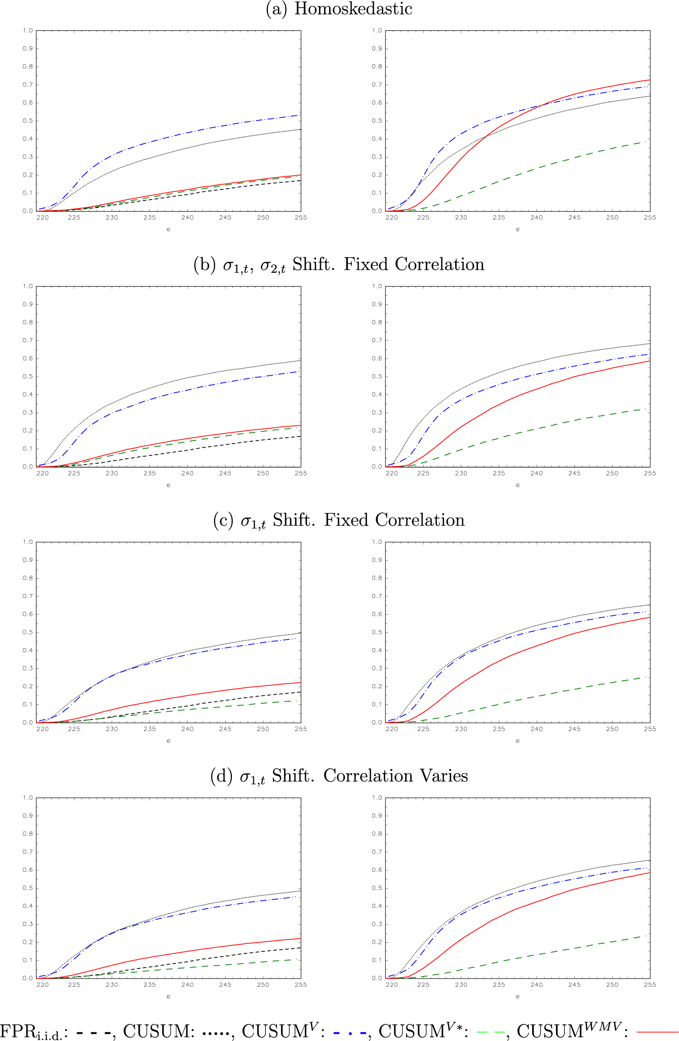 $\beta =-0.8$
,
$\beta =-0.8$
, $\rho =0.8$
,
$\rho =0.8$
, $\sigma _{12}=0.4$
, and
$\sigma _{12}=0.4$
, and $\alpha _1=0.2$
—left panel=FPR, right panel =TPR (
$\alpha _1=0.2$
—left panel=FPR, right panel =TPR ( $\varrho ^2=0.026$
).
$\varrho ^2=0.026$
).
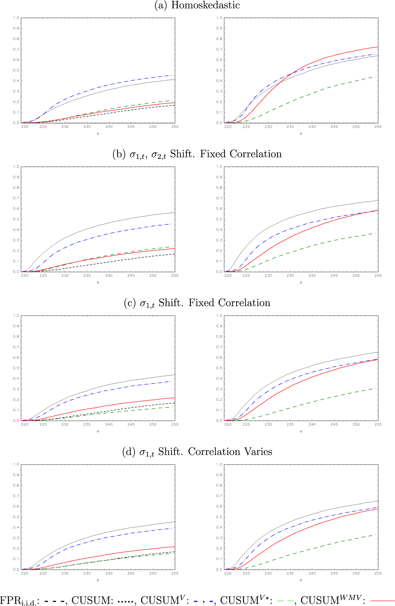
Across these figures, neither the standard CUSUM nor CUSUM $^V$
procedures exhibit controlled FPR, with both of these procedures often displaying extreme FPR distortions relative to the baseline case, where
$^V$
procedures exhibit controlled FPR, with both of these procedures often displaying extreme FPR distortions relative to the baseline case, where $v_t$
is i.i.d. While the CUSUM
$v_t$
is i.i.d. While the CUSUM $^{WMV}$
and CUSUM
$^{WMV}$
and CUSUM $^{V*}$
procedures do exhibit some slight FPR distortions relative to the case where
$^{V*}$
procedures do exhibit some slight FPR distortions relative to the case where $v_t$
is i.i.d., these FPR distortions are very modest in comparison to those exhibited by CUSUM and CUSUM
$v_t$
is i.i.d., these FPR distortions are very modest in comparison to those exhibited by CUSUM and CUSUM $^V$
. Within each figure, examining the FPR performance of the procedures across panels (b)–(d) shows that the FPR performance of the CUSUM
$^V$
. Within each figure, examining the FPR performance of the procedures across panels (b)–(d) shows that the FPR performance of the CUSUM $^{WMV}$
procedure is broadly similar in the cases where a shift in volatility occurs in
$^{WMV}$
procedure is broadly similar in the cases where a shift in volatility occurs in $\varepsilon _{1,t}$
and where a shift in volatility occurs in both
$\varepsilon _{1,t}$
and where a shift in volatility occurs in both $\varepsilon _{1,t}$
and
$\varepsilon _{1,t}$
and $\varepsilon _{2,t}$
, regardless of whether the correlation between these innovations remains fixed or not. This is not true for the remaining procedures which have an FPR profile that changes significantly across these three scenarios.
$\varepsilon _{2,t}$
, regardless of whether the correlation between these innovations remains fixed or not. This is not true for the remaining procedures which have an FPR profile that changes significantly across these three scenarios.
While we include the TPR of the standard CUSUM and CUSUM $^V$
procedures in the figures we cannot compare these directly to the TPR of CUSUM
$^V$
procedures in the figures we cannot compare these directly to the TPR of CUSUM $^{WMV}$
and CUSUM
$^{WMV}$
and CUSUM $^{V*}$
as the former two procedures display very significant FPR distortions under the null. Between the two FPR controlled procedures, the TPR of CUSUM
$^{V*}$
as the former two procedures display very significant FPR distortions under the null. Between the two FPR controlled procedures, the TPR of CUSUM $^{WMV}$
is consistently much higher than that of CUSUM
$^{WMV}$
is consistently much higher than that of CUSUM $^{V*}$
across scenarios, showing that while CUSUM
$^{V*}$
across scenarios, showing that while CUSUM $^{V*}$
is able to control the FPR under the null by dealing with the serial correlation induced by the presence of the covariate, it is unable to exploit the information from the covariate under the alternative, unlike CUSUM
$^{V*}$
is able to control the FPR under the null by dealing with the serial correlation induced by the presence of the covariate, it is unable to exploit the information from the covariate under the alternative, unlike CUSUM $^{WMV}$
which displays impressive TPR properties across all scenarios considered.
$^{WMV}$
which displays impressive TPR properties across all scenarios considered.
5.3 Summary of Additional Results in the Supplementary Material
-
1. Results for the case where a volatility shift is present in only
$\epsilon _{2,t}$
are reported in Section A.4.2 of the Supplementary Material. These highlight that the standard CUSUM procedure is unable to control the FPR as the volatility shift in the unmodeled covariate manifests in the values of
$\Delta y_t$
used to construct the CUSUM statistics. The CUSUM
$^{V}$
procedure is only able to control FPR when no serial correlation is present in
$v_t$
, and the FPR of the CUSUM
$^{V*}$
procedure, while better than that of CUSUM and CUSUM
$^{V}$
, is also quite poor. However, CUSUM
$^{WMV}$
displays good FPR control in all of the scenarios considered. -
2. Results for the case where
$x_t$
is subject to measurement error are reported in Section A.4.3 of the Supplementary Material. These suggest that while the TPR of the CUSUM
$^{WMV}$
procedure is reduced in the presence of measurement error, increasingly so as the variance of the measurement error increases, it remains superior to the TPR exhibited by the other procedures. -
3. Results where a bubble in the training sample is present in
$x_t$
are reported in Section A.4.4 of the Supplementary Material. The CUSUM
$^{V}$
procedure is unaffected, provided the bubble terminates at least H (the maximum bandwidth considered for the kernel variance estimator) periods before the start of monitoring. For CUSUM
$^{WMV}$
and CUSUM
$^{V*}$
, the residuals used in constructing the CUSUM statistics use all of the available sample data. Where the covariate is irrelevant, the FPR and TPR of the CUSUM
$^{WMV}$
and CUSUM
$^{V*}$
procedures are little altered, while a training sample bubble in a relevant covariate causes a slight inflation of the FPR of the CUSUM
$^{WMV}$
and CUSUM
$^{V*}$
procedures. This could potentially be obviated by truncation of the training sample. -
4. Results for the case where an irrelevant
$I(1)$
covariate,
$x_t$
, is mistakenly used in the CUSUM
$^{WMV}$
procedure are reported in Section A.4.5 of the Supplementary Material. These show that including
$x_t$
causes CUSUM
$^{WMV}$
to exhibit a slightly inflated FPR and modestly lower TPR than the correctly specified univariate tests. Reassuringly, the loss in TPR is modest and is predicated on a practitioner failing to difference
$ x_t$
and then forcing the inclusion of
$x_t$
in the CUSUM
$^{WMV}$
procedure, as the BIC model selection we recommend for this procedure determines
$x_t$
to be irrelevant in the vast majority of cases. -
5. Results where an irrelevant covariate admits a bubble during the monitoring period are reported in Section A.4.6 of the Supplementary Material. We consider the case where the covariate is initially either
$I(0)$
or
$I(1)$
before switching to an explosive regime at the start of monitoring. Forcibly including the covariate in the CUSUM
$^{WMV}$
procedure leads to a slight inflation of the FPR under the null and a modest decrease in the TPR under the alternative, with this effect more pronounced where the covariate is initially
$I(0) $
. Analogous results for a relevant covariate containing a bubble at the start of monitoring are reported in Section A.4.7 of the Supplementary Material. These show a very slight increase in the FPR and no perceptible change in the TPR, relative to the case where no bubble is present in the covariate. -
6. Results where a mean shift is present during the monitoring period in a utilized covariate are reported in Section A.4.8 of the Supplementary Material. These suggest that this is problematic only where the covariate is relevant (
$\beta \neq 0$
). A mean shift in a relevant covariate which is entered in first differences, as will generally be the case with macro and financial variables (see Remark 2.8), also appears relatively benign. A mean shift in a series entered in levels is more problematic causing a large increase in the FPR of CUSUM
$^{WMV}$
. However, the approach suggested at the end of Section 4 to simultaneously monitor the covariate for structural change appears useful, in that under the no bubble null it rejects in the presence of the mean shift with significantly higher frequency than does CUSUM
$^{WMV}$
. -
7. Results where a relevant but unobserved covariate,
$x_t$
, is the input to an observed local-to-unity process,
$z_t$
, with local-to-unity parameter,
$c> 0 $
, but
$\Delta z_t$
(rather than
$ z_t - ( 1- \frac {c}{T}) z_{t-1} $
) is incorrectly used as the covariate are reported in Section A.4.9 of the Supplementary Material. Relative to the correctly specified case, where
$c=0$
, the FPR of CUSUM
$^{WMV}$
tends to be slightly increased and the TPR slightly decreased, with these effects increasing in
$c $
. These findings echo the results reported in Hansen (Reference Hansen1995, pp. 1159–1160) for covariate-augmented unit root tests in this scenario. We note that
$ \Delta z_t$
does not violate the regularity conditions given in Assumption 2, regardless of the value of c.





6 CONCLUSIONS
We have developed a generalization of the univariate CUSUM-based real-time bubble monitoring procedure of HB which incorporates additional information from relevant covariates and is also robust to unconditional heteroskedasticity and serial correlation in the disturbances. We have shown that the CUSUM statistics used in this procedure follow the same limiting null distribution as those in HB, such that a monitoring procedure can be validly based on the same large sample boundary function. Monte Carlo results were presented showing that, in contrast to univariate procedures, our proposed procedure has a controlled FPR, where a relevant dynamic covariate enters the DGP. Moreover, where an explosive episode occurs in the monitoring period, incorporating the covariate can yield significant gains in finite sample detection efficacy, relative to univariate procedures. procedure. In a pseudo real-time monitoring exercise, for several plausible covariates, it would have led to an earlier rejection than the univariate procedure of AHLTZ for both the Black Monday and dotcom bubble episodes.
SUPPLEMENTARY MATERIAL
The supplementary material for this article can be found at https://doi.org/10.1017/S0266466626100383.
FUNDING STATEMENT
A.M.R.T. is grateful for research support from the Aarhus Center for Econometrics (ACE) funded by the Danish National Research Foundation grant number DNRF186. Y.Z. gratefully acknowledges financial support from the University of Macau’s APAEM Seed Grant.
COMPETING INTEREST STATEMENT
The authors declare that no competing interests exist.

















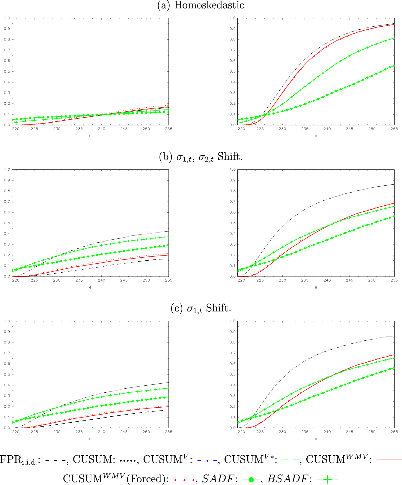


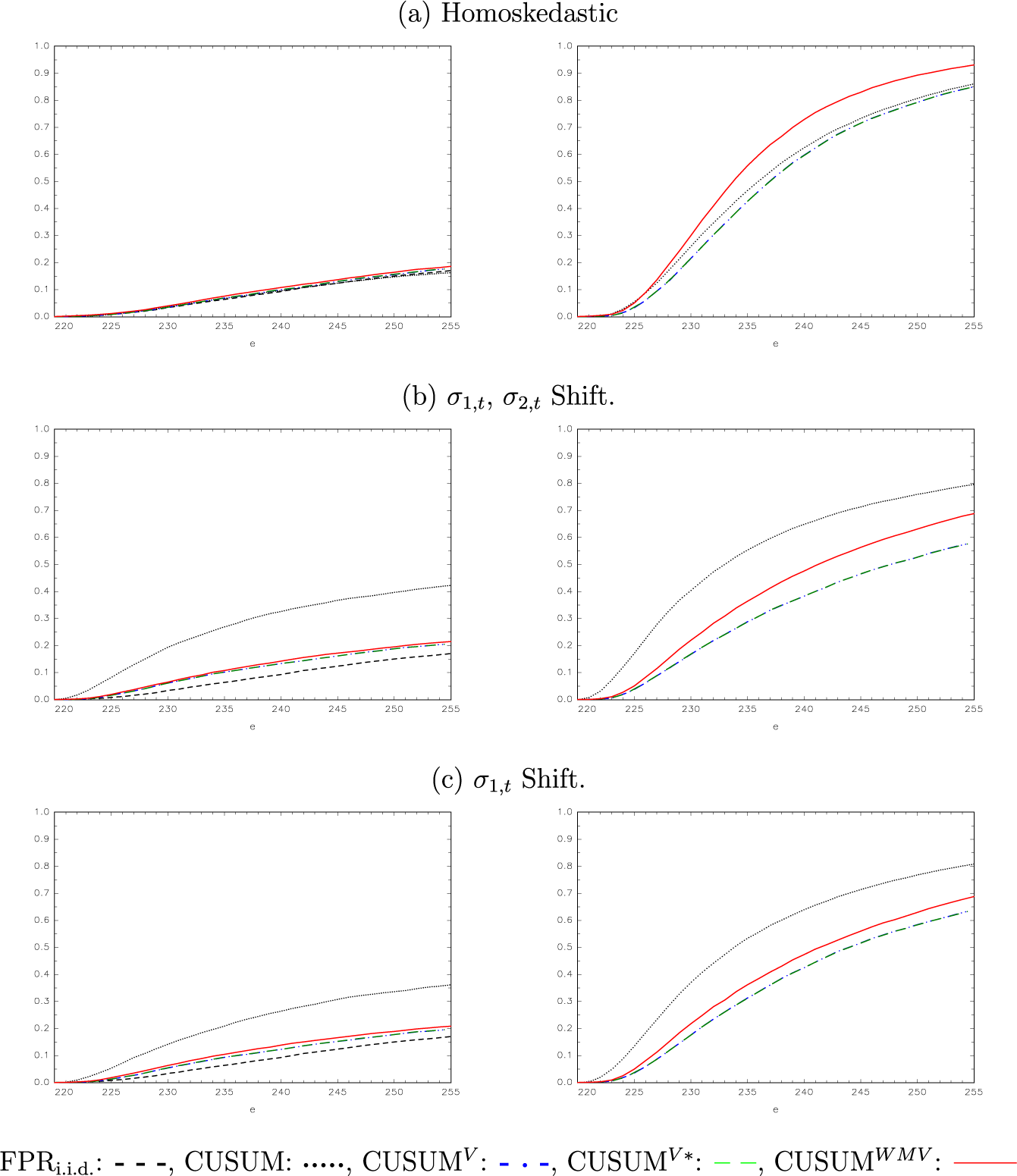


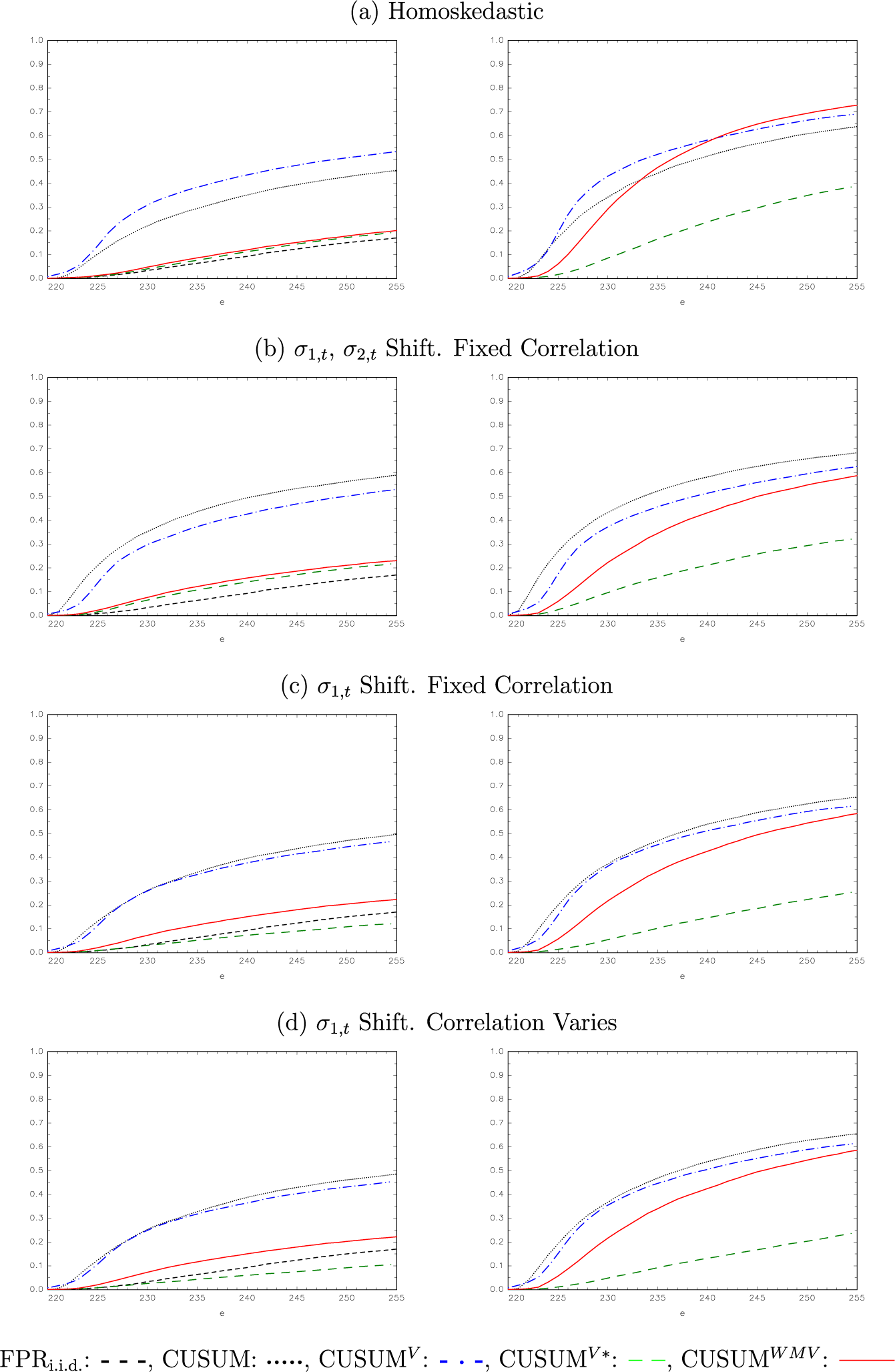


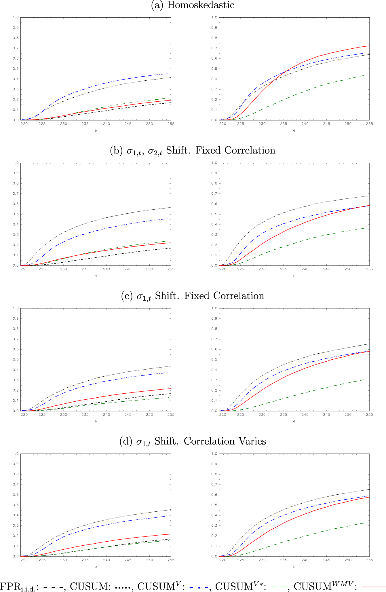


 Open access

