





1 Introduction
By the end of the 1940s, the U.S. Air Force was alarmed by an excessively high rate of incidents and accidents caused by its pilots. While investigating this issue, the Air Force identified the cockpit design as a crucial risk factor. The cockpit had originally been designed to fit the dimensions of the “average pilot” based on measurements taken in 1926. To define the “average” pilot, the U.S. Air Force instructed Lieutenant Gilbert S. Daniels to measure over 4000 pilots on 10 dimensions, including height, sleeve length, and chest circumference. Daniels computed the average for each dimension and added 15% below and above, yielding an “average window” for each dimension. At the time, most U.S. Air Force researchers expected that a sizable number of pilots would fit the average pilot definition and that they would fall into the average window in each dimension. However, of the 4063 pilots, none fit the average across all dimensions. This observation led to the conclusion that “There was no such thing as the average pilot” (Rose, Reference Rose2015).
As of then, focusing on individuals rather than averages was the approach the U.S. Air Force followed. However, in much of psychological test construction and application of tests to diagnose individuals in the clinical, educational, and personnel selection and assessment contexts, the focus is still on averages, ignoring that averages usually do not apply to individuals. The reliability of a test score is such an average, informing us of a group characteristic but not of the precision of individual test scores (e.g., Samejima, Reference Samejima1977). Consequently, the practice widely encountered of concluding from a given reliability that measurement of individuals is precise (or imprecise) is incorrect. In addition, test constructors and test practitioners sometimes use the standard error of measurement (SEM; Lord & Novick, Reference Lord and Novick1968) derived from the reliability to construct a confidence interval (CI) for the true scores the test score purports to measure. Although the SEM provides a better impression of the precision of individual test scores than the reliability, the problem is that, like the reliability, the SEM is a group characteristic, providing a single value for measurement precision that again is a group average and does not apply to individual test scores.
We therefore need a SEM that is conditional on the test score, henceforth called CSEM, which can reveal when measurement precision varies across test scores. Perhaps the call for a CSEM appears obvious, perhaps even superfluous, and indeed the Standards for Educational and Psychological Testing (AERA, APA, and NCME, 2014, Standard 2.14, p. 46) is explicit when it posits that “conditional standard errors of measurement should be reported at several score levels unless there is evidence that the standard error is constant across score levels.” However, for test constructors and test practitioners, obtaining such evidence is easier said than done, and the main reason may well be that, though methods for the CSEM were available for a long time (e.g., Mollenkopf, Reference Mollenkopf1949; Thorndike, Reference Thorndike and Lindquist1951; also, see Feldt et al., Reference Feldt, Steffen and Gupta1985, and Brennan, Reference Brennan1998, in the context of generalizability theory), they were not included in popular software packages such as IBM SPSS Statistics. According to Borsboom (Reference Borsboom2006), absence from popular software packages is detrimental for using a method at all.
We notice that in the classical test theory (CTT) context, psychometricians have paid more attention to studying the group characteristic of reliability as well as the unconditional SEM than to CSEM methods. In contrast to CSEM methods, reliability methods and corresponding SEMs have been generously included in popular software packages, suggesting why they did gain so much popularity among researchers and practitioners unlike CSEM methods that were not represented in such software packages. The absence of CSEM methods in software may also explain why available methods based on item response theory (IRT) for assessing uncertainty in person scores, present in small or relatively obscure software packages but not in the big popular packages, never became as popular as classical reliability and the corresponding SEM. In this article, we present software implemented in software package JASP (JASP Team, 2024) that enables researchers to estimate several CSEM methods based on classical test theory (CTT) and item response theory (IRT).
To summarize, we think it should come as no surprise that test constructors and test practitioners who are testing patients, students, and applicants individually, and who are not backed up by a large testing agency with its own psychometric support team, usually rely on group-based reliability information and, if they do, use the common SEM. Hence, we do not claim that test constructors and test users are not prepared to take responsibility to use nuanced psychometric methods, but rather that despite their existence such methods are relatively obscure in the literature and often unavailable in popular software, and therefore are hardly used.
1.1 What is the problem?
Outside of psychometrics, it is a little known fact that a test with a high reliability may produce imprecise test scores for some test-takers leaving much uncertainty about their true scores, and conversely, that an unreliable test may produce some precise test scores representing their true scores well (see, e.g., Stanley & Spence, Reference Stanley and Spence2024, for a recent example). Some individuals may obtain test scores suffering from low precision even when the test score has an overall reliability as high as 0.9. In contrast, others may obtain test scores with high precision when the test has an overall reliability equal to a modest 0.6. The problem is that reliability is a group characteristic, expressing the proportion of test-score variance in the group that is true-score variance. A reliability of 0.9 thus means that 90% of the variance in the test scores is due to differences in the true scores, while a value of 0.6 means that 60% of the test-score variance is due to true-score variance. The definition of reliability therefore implies that we only know that if reliability equals, say, 0.9, variation in the true scores is almost (but not) as large as the variation in the test scores meaning that most (but not necessarily all) test scores are close to the corresponding true scores, and if reliability is 0.6, variation in true scores is quite a bit smaller meaning that test scores and true scores are often dissimilar, though some may be quite close. Thus, reliability only provides group-level information about the ratio of true-score and test-score variance, and we hope the reader understands that reliability does not tell us a lot about the precision with which Mary’s test score estimates her true score or whether Mary’s and John’s true scores are really different even when their observable test scores are. The same point can be made when comparing test scores with a cut score: If reliability equals 0.8, the cut score is 25, and John’s test score is 26, can we conclude that John’s true score is higher than 25? Based on only this information, we cannot. Reliability informs us of the relative variance of the true scores in the group, but not of the precision of individual test scores.
In the event that researchers or practitioners actually are interested to know more of the precision of individual test scores as estimates of the corresponding true scores, it is wry that they usually employ the SEM, which does not provide them with the precision of test scores as estimates of corresponding true scores. The reason is that, because the SEM depends on the reliability and the variance of the test scores, two quantities that only are informative of the group, the SEM is also a group characteristic. Users of the SEM assume, either for practical reasons or due to ignorance, that its value is valid for all test scores, suggesting that measurement precision is the same along the whole scale. Usually, it is not. Interestingly, psychometricians provided the methodology for the estimation of conditional measurement precision already quite a few decades ago (Mollenkopf, Reference Mollenkopf1949; Thorndike, Reference Thorndike and Lindquist1951; also, see Feldt et al., Reference Feldt, Steffen and Gupta1985; Feldt & Qualls, Reference Feldt and Qualls1996; Jarjoura, Reference Jarjoura1986; Lord, Reference Lord1984; Woodruff, Reference Woodruff1990, Reference Woodruff1991) and also more recently kept arguing to adopt the methodology (Embretson, Reference Embretson1996; Lek & Van De Schoot, Reference Lek and Van de Schoot2018; McNeish & Dumas, Reference McNeish and Dumas2025; Waller & Reise, Reference Waller and Reise1989), but despite the effort, conditional measurement precision has not become part of the standard psychometric toolkit. Two problems are that (1) nontechnical literature informing nonpsychometricians about conditional measurement precision and emphasizing its importance was hardly available and, related to this scarcity, that (2) accessible software that allows easily obtainable conditional measurement–precision estimates was nonexistent.
In this focus article, we alleviate both problems by discussing multiple methods to obtain conditional measurement–precision estimates in a nontechnical manner and by implementing the methods in accessible software, which is the open access software package JASP (JASP Team, 2024). The methods fall into two classes both based on CTT (i.e., split-test and analysis of variance [ANOVA] procedures) and one class based on IRT. Methods are suited for both polytomous (e.g., rating-scale scores) and dichotomous (e.g., incorrect/correct scores) data, unless indicated otherwise. Using a real-data example, we demonstrate how to obtain estimates for conditional measurement precision from JASP software, and we guide the reader through the use of these conditional methods. If readers prefer to use their own code, they can ignore the JASP software. Statistical details can be found in the Appendix.
1.2 A real-data example of an ADHD symptom scale
The following real-data example highlights the importance of conditional precision expressed by the CSEM over overall precision expressed by the SEM. The case serves as a running example throughout the text. The sample consists of children ( $N=1,166$
; after removal of four incomplete data lines,
$N=1,166$
; after removal of four incomplete data lines, ${N}_{\mathrm{complete}}=1,162$
) who were rated by their parents on 18 five-point Likert scale items, together addressing each of the DSM-5 ADHD symptoms (Keulers & Hurks, Reference Keulers and Hurks2021). The ordered response categories represent the prevalence of a specific symptomatic behavior, scored from 0 (never) to 4 (very often). For the ADHD scale, the test score is the sum of the individual item scores, and a higher sum score indicates more ADHD symptoms, some of which may be more extreme. The 18 items can be separated into two subscales, one subscale measuring nine attention symptoms and the other nine hyperactivity–impulsivity symptoms. For the purpose of illustration, we will only consider the first subscale measuring attention symptoms, and henceforth call it the ADD scale. With nine items, the sum score on the ADD scale ranges from 0 to 36. The mean of the sum scores equals 11.6 (SD = 6.4) and the estimated test score reliability by means of coefficient
${N}_{\mathrm{complete}}=1,162$
) who were rated by their parents on 18 five-point Likert scale items, together addressing each of the DSM-5 ADHD symptoms (Keulers & Hurks, Reference Keulers and Hurks2021). The ordered response categories represent the prevalence of a specific symptomatic behavior, scored from 0 (never) to 4 (very often). For the ADHD scale, the test score is the sum of the individual item scores, and a higher sum score indicates more ADHD symptoms, some of which may be more extreme. The 18 items can be separated into two subscales, one subscale measuring nine attention symptoms and the other nine hyperactivity–impulsivity symptoms. For the purpose of illustration, we will only consider the first subscale measuring attention symptoms, and henceforth call it the ADD scale. With nine items, the sum score on the ADD scale ranges from 0 to 36. The mean of the sum scores equals 11.6 (SD = 6.4) and the estimated test score reliability by means of coefficient $\alpha$
equals 0.88.
$\alpha$
equals 0.88.
Figure 1 (left-hand panel) shows the SEM, which is necessarily equal for all ADD sum scores and suggests that measurement precision, here more than 2 scale units, is the same along the whole scale. Despite the use of the SEM, there exists some common lore that psychological tests are not equally precise for each individual tested, therefore that the situation in the left-hand panel of Figure 1 is unrealistic, hence misleading. For example, for someone not suffering from ADHD, the symptoms are absent, and therefore, we expect high measurement precision (small CSEM) for low ADD sum scores (no ADHD), whereas someone suffering from medium ADHD, thus obtaining a higher sum score, is measured with lower precision (larger CSEM). The underlying explanation is that symptom extremity may vary across repeated measurement, but less so (in this example) at the lower end of the scale (no ADHD). Figure 1 (right-hand panel) shows this phenomenon, and is consistent with the psychometric literature that measurement precision is highest at the endpoints of a scale and lowest around the middle (Feldt et al., Reference Feldt, Steffen and Gupta1985; Feldt & Qualls, Reference Feldt and Qualls1996; Lee et al., Reference Lee, Brennan and Kolen2000). We notice this phenomenon depends on the, apparently common, item composition of the test and may be different for different compositions, but we will leave this topic alone.
SEM and CSEM for the ADD data.
Note: In the traditional approach, all test scores have the same SEM value. When estimating the SEM for each test sum score, individuals with a high or low score are measured with less error than individuals with a median score.

Based on the same data as Figure 1, Figure 2 (left-hand panel) shows the equally wide CIs for the true scores based on the SEM. Because the SEM has the same value for each sum score, a little over 2 scale units, 95% CIs have a width over 8 scale units, equal for all sum scores. The right-hand panel shows the CIs with varying widths based on the CSEM. Hence, the CSEM reveals that some ADD sum scores are more precise true-score estimates than others, whereas the SEM obscures this reality. Suppose, we use a cutoff equal to 12 on the ADD scale to assign children to therapy (when they score above the cutoff), and this is the only source of information we use (admitted not very realistic in practice, but useful for our line of reasoning). Then, we might decide that sum scores higher than 12, of which the accompanying CIs do not include score 12, provide enough evidence that their corresponding true scores are greater than the cutoff. Inspecting the sum scores and CIs in Figure 2, we find that in the unconditional case (left panel) the CI of the sum score of 17 is the first not to include the cutoff. In the conditional approach (right panel), the CI for the sum score of 17 does include the cutoff, and hence we would start at a sum score of 18 to assign children to therapy (again, this is only a hypothetical example). Wider CIs imply more leniency and narrower CIs imply more strictness, but using the SEM (left-hand panel) leaves the practitioner in the dark about such issues.
95% CIs using the SEM and the CSEM around the true score estimate for the ADD data.
Note: In the unconditional approach, the CIs around the true score estimate are all created with the same SEM value. For illustration, we drew a dotted line at a hypothetical cutoff score of 12. In the conditional approach, the CIs are created with a dedicated SEM value for each sum score unless the sum score group was too small, that is, for sum scores with a small number of observations (<20), we grouped adjacent sum scores together (see sum scores of 28 and above in the plot).

2 Classical test theory, reliability, and measurement precision
Following CTT, one assumes that the test score, $X$
, is the sum of a true score,
$X$
, is the sum of a true score, $T$
, and random measurement error,
$T$
, and random measurement error, $E$
, so that
$E$
, so that $X=T+E$
(Lord & Novick, Reference Lord and Novick1968). Measurement error introduces uncertainty in a person’s test performance, irrespective of what the test performance represents. CTT focuses on reliability and precision of the test score, while the meaning of the test performance is the domain of validity research. Although methods such as IRT take better advantage of statistical theory and provide more nuances than CTT (but without contradicting CTT; Lord, Reference Lord1980), CTT remains popular among researchers, test constructors, and test practitioners, probably because of its simplicity, but also because it focuses on the appealing test-score property of reliability, even if that is not always well understood.
$X=T+E$
(Lord & Novick, Reference Lord and Novick1968). Measurement error introduces uncertainty in a person’s test performance, irrespective of what the test performance represents. CTT focuses on reliability and precision of the test score, while the meaning of the test performance is the domain of validity research. Although methods such as IRT take better advantage of statistical theory and provide more nuances than CTT (but without contradicting CTT; Lord, Reference Lord1980), CTT remains popular among researchers, test constructors, and test practitioners, probably because of its simplicity, but also because it focuses on the appealing test-score property of reliability, even if that is not always well understood.
2.1 Reliability
In the model equation, $X=T+E$
, only the sum score is observable, but the true score and the measurement error are not. This poses problems for the estimation of reliability. This is why the lion’s share of psychometric work in CTT has been devoted to finding indirect methods to estimate reliability. The most popular method is coefficient
$X=T+E$
, only the sum score is observable, but the true score and the measurement error are not. This poses problems for the estimation of reliability. This is why the lion’s share of psychometric work in CTT has been devoted to finding indirect methods to estimate reliability. The most popular method is coefficient $\alpha$
(Cronbach, Reference Cronbach1951; Sijtsma & Pfadt, Reference Sijtsma and Pfadt2021a), but many other methods are available (e.g., Cho, Reference Cho2016). In real test data, such indirect methods are approximations to reliability, but they are often close enough to be useful, especially when the items measure the same attribute except for some small deviations.
$\alpha$
(Cronbach, Reference Cronbach1951; Sijtsma & Pfadt, Reference Sijtsma and Pfadt2021a), but many other methods are available (e.g., Cho, Reference Cho2016). In real test data, such indirect methods are approximations to reliability, but they are often close enough to be useful, especially when the items measure the same attribute except for some small deviations.
To understand how reliability is related to the SEM, we first need to define reliability and then proceed to define the SEM. Let Greek lower case rho ( $\rho$
) denote reliability, and let the variances of test score
$\rho$
) denote reliability, and let the variances of test score $X$
, true score
$X$
, true score $T$
, and error
$T$
, and error $E$
be denoted by
$E$
be denoted by ${\sigma}_X^2$
,
${\sigma}_X^2$
, ${\sigma}_T^2$
, and
${\sigma}_T^2$
, and ${\sigma}_E^2$
; then, assuming error covaries zero with true scores, reliability is defined as
${\sigma}_E^2$
; then, assuming error covaries zero with true scores, reliability is defined as
 $$\begin{align}\rho =\frac{\sigma_T^2}{\sigma_X^2}=1-\frac{\sigma_E^2}{\sigma_X^2}.\end{align}$$
The first fraction is the proportion of test-score variance ( ${\sigma}_X^2$
) that is true-score variance (
${\sigma}_X^2$
) that is true-score variance ( ${\sigma}_T^2$
), and the last equation is one minus the proportion of test-score variance (
${\sigma}_T^2$
), and the last equation is one minus the proportion of test-score variance ( ${\sigma}_X^2$
) that is error variance (
${\sigma}_X^2$
) that is error variance ( ${\sigma}_E^2$
) or, equivalently, the proportion of test-score variance not attributable to error variance.
${\sigma}_E^2$
) or, equivalently, the proportion of test-score variance not attributable to error variance.
We need only one step to the SEM, which entails rewriting Equation (1) to the error variance, so that
 $$\begin{align}{\sigma}_E^2={\sigma}_X^2\left(1-\rho \right),\end{align}$$
and then taking the square root of both sides and calling the result the SEM,
 $$\begin{align}{\sigma}_E=\mathrm{SEM}={\sigma}_X\sqrt{\left(1-\rho \right)}.\end{align}$$
Three comments are in order. First, because true score $T$
and measurement error
$T$
and measurement error $E$
are unobservable, their variances
$E$
are unobservable, their variances ${\sigma}_T^2$
and
${\sigma}_T^2$
and ${\sigma}_E^2$
are unobservable as well (Equation (1)), so that reliability
${\sigma}_E^2$
are unobservable as well (Equation (1)), so that reliability $\rho$
cannot be estimated directly. Because the SEM is a simple rewrite of the reliability, the SEM cannot be computed directly from test data, because
$\rho$
cannot be estimated directly. Because the SEM is a simple rewrite of the reliability, the SEM cannot be computed directly from test data, because $\rho$
cannot be estimated directly (Equation (3)). Hence, we have to insert an approximation for reliability
$\rho$
cannot be estimated directly (Equation (3)). Hence, we have to insert an approximation for reliability $\rho$
based on observable quantities in Equation (3) to obtain the SEM.
$\rho$
based on observable quantities in Equation (3) to obtain the SEM.
Second, because the reliability consists of two group quantities, ${\sigma}_T^2$
and
${\sigma}_T^2$
and ${\sigma}_X^2$
, it is also a group characteristic uninformative of individual scores, and the same is true of its rewrite, the SEM. This does not affect the observation that different educational tests of the same length but varying standard deviation
${\sigma}_X^2$
, it is also a group characteristic uninformative of individual scores, and the same is true of its rewrite, the SEM. This does not affect the observation that different educational tests of the same length but varying standard deviation ${\sigma}_X$
and reliability
${\sigma}_X$
and reliability $\rho$
tend to have SEMs that show little variation. The reason is that a higher standard deviation
$\rho$
tend to have SEMs that show little variation. The reason is that a higher standard deviation ${\sigma}_X$
tends to go together with increasing reliability
${\sigma}_X$
tends to go together with increasing reliability $\rho$
, hence decreasing
$\rho$
, hence decreasing $\sqrt{\left(1-\rho \right)}$
, thus counteracting one another producing the SEM (Lord, Reference Lord1957). Based on one dataset, Blixt and Shama (Reference Blixt and Shama1986) even concluded that Equation (3) should be preferred to CSEMs, but this conclusion appears obsolete given evidence accumulated since.
$\sqrt{\left(1-\rho \right)}$
, thus counteracting one another producing the SEM (Lord, Reference Lord1957). Based on one dataset, Blixt and Shama (Reference Blixt and Shama1986) even concluded that Equation (3) should be preferred to CSEMs, but this conclusion appears obsolete given evidence accumulated since.
Third, the SEM obscures a result well known from the psychometric literature (e.g., Mellenbergh, Reference Mellenbergh1996; Sijtsma & Van der Ark, Reference Sijtsma and van der Ark2021, p. 74), which is that the squared SEM, ${\sigma}_E^2$
, is the mean of the error variances of all individual population members. That is, indexing individuals by
${\sigma}_E^2$
, is the mean of the error variances of all individual population members. That is, indexing individuals by $i$
and their error variances by
$i$
and their error variances by ${\sigma}_{E_i}^2$
,
${\sigma}_{E_i}^2$
,
 $$\begin{align}{\sigma}_E^2=\mathbb{E}\left({\sigma}_{E_i}^2\right),\end{align}$$
where $\mathbb{E}$
stands for expectation. Equation (4) shows precisely what the problem is with measurement precision using the SEM from Equation (3): By acknowledging that error variance can be different for different individuals, we would rather use a CSEM,
$\mathbb{E}$
stands for expectation. Equation (4) shows precisely what the problem is with measurement precision using the SEM from Equation (3): By acknowledging that error variance can be different for different individuals, we would rather use a CSEM, ${\sigma}_{E_i}$
, but the SEM,
${\sigma}_{E_i}$
, but the SEM, ${\sigma}_E$
, only provides us with the mean of all
${\sigma}_E$
, only provides us with the mean of all ${\sigma}_{E_i}^2$
s. In practice, it is impossible to estimate
${\sigma}_{E_i}^2$
s. In practice, it is impossible to estimate ${\sigma}_{E_i}$
for each person. Instead, one focuses on the test score. Then, the SEM obscures the differences needed for identifying which test scores are precise and which test scores are not. Because use of the SEM has become the rule rather than the exception, we first say a little more about it before we move to the more realistic CSEM.
${\sigma}_{E_i}$
for each person. Instead, one focuses on the test score. Then, the SEM obscures the differences needed for identifying which test scores are precise and which test scores are not. Because use of the SEM has become the rule rather than the exception, we first say a little more about it before we move to the more realistic CSEM.
2.2 Standard error of measurement
For the ADD data, we computed the sample standard deviation of the sum scores, which equals 6.36, and we approximated $\rho$
with coefficient
$\rho$
with coefficient $\alpha$
and found estimate
$\alpha$
and found estimate $\widehat{\alpha}=0.88$
. Inserting these two quantities in Equation (3), we obtain the estimate of the SEM,
$\widehat{\alpha}=0.88$
. Inserting these two quantities in Equation (3), we obtain the estimate of the SEM, $\widehat{\mathrm{SEM}}=2.18$
. To obtain the CI, we take the following steps. First, we assume that errors are normally distributed. Second, for a 95% CI, we use the
$\widehat{\mathrm{SEM}}=2.18$
. To obtain the CI, we take the following steps. First, we assume that errors are normally distributed. Second, for a 95% CI, we use the $z$
scores that correspond to the
$z$
scores that correspond to the $0.025$
and
$0.025$
and $0.975$
percentiles of the standard normal distribution, which are
$0.975$
percentiles of the standard normal distribution, which are ${z}_{0.025}=-1.96$
and
${z}_{0.025}=-1.96$
and ${z}_{0.975}=1.96$
. Third, we multiply the
${z}_{0.975}=1.96$
. Third, we multiply the $\widehat{\mathrm{SEM}}$
by
$\widehat{\mathrm{SEM}}$
by ${z}_{0.05}$
and
${z}_{0.05}$
and ${z}_{0.975},$
respectively, and obtain the lower and upper bounds of the CI:
${z}_{0.975},$
respectively, and obtain the lower and upper bounds of the CI:
 $$\begin{align}\left[{z}_{0.05}\times \widehat{\mathrm{SEM}};{z}_{0.975}\times \widehat{\mathrm{SEM}}\right].\end{align}$$
For any sum score, thus also including a sum score of 12, $\widehat{\mathrm{SEM}}=2.18$
, we obtain the CI as
$\widehat{\mathrm{SEM}}=2.18$
, we obtain the CI as $\left[12\pm 1.96\times 2.18\right]$
, resulting in [7.72, 16.27]. The width of the CI, here 8.55 units, is assumed the same for each sum score. The location of the CI is the only feature that varies with the sum score. For example, for a sum score of 15, the CI shifts 3 units to the right, but its width remains 8.55 units.
$\left[12\pm 1.96\times 2.18\right]$
, resulting in [7.72, 16.27]. The width of the CI, here 8.55 units, is assumed the same for each sum score. The location of the CI is the only feature that varies with the sum score. For example, for a sum score of 15, the CI shifts 3 units to the right, but its width remains 8.55 units.
Introducing conditional measurement precision quantified by CSEM, we obtain CIs that also vary with respect to width for different sum scores, as Figure 2 showed. For the sum score of 12, as we explain later, $\widehat{\mathrm{CSEM}}=2.23$
, and for the next sum score of 13,
$\widehat{\mathrm{CSEM}}=2.23$
, and for the next sum score of 13, $\widehat{\mathrm{CSEM}}=2.3$
. The corresponding CIs are
$\widehat{\mathrm{CSEM}}=2.3$
. The corresponding CIs are $\left[12\pm 1.96\times 2.23\right]$
, which equals
$\left[12\pm 1.96\times 2.23\right]$
, which equals $\left[7.63,16.37\right]$
; and
$\left[7.63,16.37\right]$
; and $\left[13\pm 1.96\times 2.3\right]$
, which equals
$\left[13\pm 1.96\times 2.3\right]$
, which equals $\left[8.49,17.51\right]$
. Their widths differ only 0.28 units, probably because the scores are neighbors on the sum-score scale, still expressing a little more certainty for the first true score. Across the scale we often expect larger differences in measurement precision, but the subtle difference in the example illustrates a core advantage of the CSEM: It captures variation in measurement precision that the common unconditional SEM ignores.
$\left[8.49,17.51\right]$
. Their widths differ only 0.28 units, probably because the scores are neighbors on the sum-score scale, still expressing a little more certainty for the first true score. Across the scale we often expect larger differences in measurement precision, but the subtle difference in the example illustrates a core advantage of the CSEM: It captures variation in measurement precision that the common unconditional SEM ignores.
3 Estimating conditional standard error of measurement for real data
In the next sections, we discuss how to obtain the various CSEM methods that we implemented in JASP. R-code to obtain the SEM methods can be found in the associated open-science repository under https://osf.io/vfyt3. All methods are mathematically correct, and their usefulness depends mostly on the intention of the user, the particular test, and the population under study. To keep the section nontechnical as much as is possible with a technical topic, we refrain from discussing equations for the various methods in the main text, but refer to the Appendix for more details.
3.1 JASP software
JASP is an open-source and free-of-charge statistical program that is developed at the University of Amsterdam. JASP is used throughout the human sciences. It can be downloaded from https://jasp-stats.org/download/. After installation, users should open JASP and load a data file. For the analysis of the ADD scale data, readers can find the ADD data file in the data library in JASP (Open > Data Library > Reliability > ADD example). The SEM analysis can be found in the reliability module, which can be accessed by opening the side panel (Figure 3, click on the blue “+” symbol in the upper right corner). The reliability module then shows up in the top analysis panel, and clicking on it shows various analyses for quantifying measurement error, such as reliability and intraclass correlation. If users choose “Standard Error of Measurement,” the analysis will open (Figure 3). Typical of JASP, the top of the analysis window contains the variables users can choose for the analysis by dragging them to the “Variables” window. The variables (here, items) need to be polytomously or dichotomously scored. Below the Variables section, users find the methods that they can select, starting with the methods based on CTT. If variables are entered into the analysis but none of the methods are selected, JASP will provide the $\widehat{\mathrm{SEM}}$
by default estimating and using coefficient
$\widehat{\mathrm{SEM}}$
by default estimating and using coefficient $\alpha$
as the reliability approximation (Figure 3). In the section “Options,” users can specify a reliability value (the box “User defined reliability”) they obtained, for example, from a test manual or having estimated using a method other than coefficient
$\alpha$
as the reliability approximation (Figure 3). In the section “Options,” users can specify a reliability value (the box “User defined reliability”) they obtained, for example, from a test manual or having estimated using a method other than coefficient $\alpha$
.
$\alpha$
.
The main SEM analysis in JASP.
Note: The left-hand side of the JASP window shows the variables and analysis options; the right-hand side shows the results. The coefficients on the left are separated into split-test methods, the ANOVA, and the IRT method, and, for dichotomous data only, the binomial methods. Having selected none of the coefficients, the analysis only estimates the SEM for the nine items of the ADD data.

3.2 Classical test theory methods
In this section, we distinguish four CTT-based approaches to CSEM. Three methods fall under the heading of split-test methods, and the fourth method is based on ANOVA.
3.2.1 Split-test methods
A common principle among the split-test methods is that they approximate the unknown conditional error variances using the variances of the difference between the sum scores on two equally sized test parts (Feldt & Qualls, Reference Feldt and Qualls1996). If measurement precision were perfect, this variance would be zero, indicating no error variance. If measurement precision is not perfect, individuals often score differently on different test parts.
Thorndike method. Using the Thorndike method (Thorndike, Reference Thorndike and Lindquist1951), we split the test into two halves, compute the sum scores of all individuals on the two test halves, and also the difference between the two half-test sum scores. For a subgroup having the same sum score on the whole test, we then estimate the variance of these difference scores. Under strict assumptions pertaining to the comparability of the two test halves (not to be discussed here), the variance of the difference scores on the test halves equals the error variance in the subgroup of persons having the same sum score on the whole test. The square root equals the Thorndike method for estimating $\mathrm{CSEM}$
; for details, see the Appendix. A CSEM is estimated for each sum-score group based on the whole test, resulting in a quantity that varies across sum scores.
$\mathrm{CSEM}$
; for details, see the Appendix. A CSEM is estimated for each sum-score group based on the whole test, resulting in a quantity that varies across sum scores.
Different splits in test halves produce different results. In the JASP implementation, based on the administration order of the items, by default the items are split into odd- and even-numbered items. For the ADD data, this means that the first, third, fifth, seventh, and ninth items are in one part, and the remaining items are in the other part. However, we encourage users to make an informed choice on how to split their test, for example, if possible, by dividing items across parts such that pairs of items from different parts match as much as possible by content. If users wish to split the items other than the default option, they need to readjust the order of the items in the variables window. For example, if two items are similar by content and they need to land in different parts, they could be the first and second items in the variables window. Another example is preferring items 1–5 in one part and items 6–9 in the other part, then the items must be ordered as 1, 6, 2, 7, 3, 8, 4, 9, 5. For the ADD data, we left the default split in place.
When the total number of items is odd, as with the ADD data, the first half contains the greater number of items, but the Thorndike method assumes an equal number of items in the test halves. For an odd number of items, Feldt and Qualls (Reference Feldt and Qualls1996) proposed to omit an item and correct the resulting statistic. However, in this specific situation with already a limited number of items, we are hesitant to leave items out of the analysis. However, we verified by simulations that this small difference of the number of items in the two parts has little to no effect on the result. In addition, for the remaining methods, an odd number of items is less of an issue as will be clear in what follows. In practice, one may want to (1) keep the imbalance to a minimum (i.e., only one item difference between the test parts); and (2) establish robustness of the results by omitting a different item in multiple runs of the analysis.
As an example, for the ADD, 68 individuals had a sum score of $9$
. For each individual, we computed the difference between their sum scores on the first test part (the odd-numbered items) and the second test part (the even-numbered items). Estimating the standard deviation of the 68 difference scores, we obtained a CSEM of (in JASP jargon)
$9$
. For each individual, we computed the difference between their sum scores on the first test part (the odd-numbered items) and the second test part (the even-numbered items). Estimating the standard deviation of the 68 difference scores, we obtained a CSEM of (in JASP jargon) $\mathrm{Thorndike}=2.66$
. By checking the “Thorndike” box, JASP produced a table with the Thorndike method CSEMs (Figure 4).
$\mathrm{Thorndike}=2.66$
. By checking the “Thorndike” box, JASP produced a table with the Thorndike method CSEMs (Figure 4).
The CSEM table in JASP.
Note: The sum score column contains the observed sum scores; the counts column provides the frequency of each sum score in the ADD dataset. The remaining columns contain the different CSEM methods for polytomous data. In JASP, the GRM is chosen as the appropriate IRT model for polytomous data. The IRT-GRM method does not yield a SEM for a sum score of 0. The $\mathrm{SEM}$
value can be found in the table note.
$\mathrm{SEM}$
value can be found in the table note.

Frequently, some sum scores are obtained only by a few individuals, posing a problem for precise SEM estimation. This happens regularly in small samples for extreme sum scores, but it can also happen for intermediate sum scores, especially when the score range is large. JASP provides the counts for each score group in the main output table (Figure 4). Inspecting Figure 4, we learn that few persons have ADD scores greater than 27. Since estimating a CSEM for a low-frequency score group would result in an unstable result, we implemented a solution suggested in the context of Mokken scale analysis (Sijtsma & Molenaar, Reference Sijtsma and Molenaar2002, p. 41). This solution entails combining neighboring low-frequency score groups into one score group, starting with the group having the smallest test score and continuing to merge next groups until a minimum group size is realized. This combined group then passes for a homogeneous sum-score group. In JASP, the user defines a minimum group size. This option can be found in the “Options” pane as “Minimum number of observations per group” (Figure 3). The default value we chose is 20. Figure 4 shows that all sum scores above 27 were combined into one score group.
If users wish to apply the CSEM values to produce CIs for each true score, they can do so in two ways: (1) Within the “Options” pane, they can find a checkbox to display a table with the sum scores and the corresponding CIs for each chosen CSEM method; or (2) within the “Plots” pane they find a checkbox (“Sum score plots”) that allows them to produce a plot of the sum scores with the CIs for each method much like the plot on the right-hand panel of Figure 2. In addition, within the “Plots” pane they can plot the CSEM values for each method by choosing “Plot per method.”
Compared to other CSEM methods, the Thorndike method (Thorndike, Reference Thorndike and Lindquist1951) is particularly effective for dichotomous item scores (Feldt et al., Reference Feldt, Steffen and Gupta1985; Feldt & Qualls, Reference Feldt and Qualls1996). Woodruff (Reference Woodruff1990) suggested that split-test methods such as the Thorndike method tend to overestimate the population SEM since they are based on the observed score rather than the true score. However, the overestimation diminishes for test with higher reliability (Feldt & Qualls, Reference Feldt and Qualls1996) and by using multiple splits (see next). In addition, Feldt et al. (Reference Feldt, Steffen and Gupta1985) and Qualls-Payne (1992) suggested that the bias is probably small, and Van der Ark et al. (Reference Van der Ark, Emons and Sijtsma2025; also, Mellenbergh, Reference Mellenbergh1996) argue this is a statistically sound method for estimating the true score. In the Appendix, we discuss Woodruff’s account in more depth.
Feldt method. The second split-test method is a combination of Thorndike’s approach and an approach Mollenkopf (Reference Mollenkopf1949) suggested, and that Feldt and Qualls (Reference Feldt and Qualls1996) developed further. Instead of splitting the test into two parts, it is split into multiple parts. Using multiple test parts reduces the influence of sampling error on the CSEM value, results in more precise estimates (Feldt & Qualls, Reference Feldt and Qualls1996). Feldt and Qualls (Reference Feldt and Qualls1996) suggested using as many parts as possible to decrease the sampling fluctuations as much as possible and recommended that test parts contain an equal number of items, and—as already mentioned above—omit as few items as possible if the test is not divisible into equally sized parts. To prevent the overestimation (Woodruff, Reference Woodruff1990, see earlier), our advice is to balance the number of items and number of test parts. That is, the number of test parts and number of items within each part should be as close together as possible. For instance, a test of 40 items is ideally split into 5 parts with 8 items each. Lee et al. (Reference Lee, Brennan and Kolen2000) found that the Feldt method performed well when the items of the test had similar content.
Using the Feldt method on the ADD data, we split the test into multiple parts, and obtained individual estimates of the error variance that we averaged to approximate the error variance for a specific sum score on the whole test (for details, see the Appendix). Using JASP, we estimated the Feldt-method CSEM by checking the “Feldt” box. Inspecting Figure 4, we found that a test score of 9 yields (in JASP jargon) $\mathrm{Feldt}=2.19$
. The “Number of splits” field below the Feldt checkbox enables the user to specify the number of parts into which the test must be split. We partitioned the nine-item ADD into as many parts as it has items, thus resulting in nine parts. Also, for the Feldt method, JASP splits the items to yield similar parts by default following the order in which the items appear in the data file. For nine items and three splits, items 1, 4, and 7 are in the first, items 2, 5, and 8 in the second, and items 3, 6, and 9 in the third test part. Users can overrule this default split using the logic discussed previously.
$\mathrm{Feldt}=2.19$
. The “Number of splits” field below the Feldt checkbox enables the user to specify the number of parts into which the test must be split. We partitioned the nine-item ADD into as many parts as it has items, thus resulting in nine parts. Also, for the Feldt method, JASP splits the items to yield similar parts by default following the order in which the items appear in the data file. For nine items and three splits, items 1, 4, and 7 are in the first, items 2, 5, and 8 in the second, and items 3, 6, and 9 in the third test part. Users can overrule this default split using the logic discussed previously.
Mollenkopf–Feldt method. The third split-test method is a polynomial regression approach suggested by Mollenkopf (Reference Mollenkopf1949) and later developed further by Feldt and Qualls (Reference Feldt and Qualls1996). The Mollenkopf method predicts the variance of the difference between test-half scores using a polynomial regression function (see the Appendix). By using a regression function with higher degree polynomials, this approach accounts for variation in difference scores more effectively, yielding smoother estimates of CSEM values (Feldt & Qualls, Reference Feldt and Qualls1996). Compared to the previous split-test methods, the Mollenkopf–Feldt method is expected to yield CSEM values with greater precision by predicting the difference scores of the test parts using a regression curve instead of just using the raw difference scores. Feldt and Qualls (Reference Feldt and Qualls1996) extended the method to split the test not only in halves but multiple test parts, similar to the Feldt method. Feldt et al. (Reference Feldt, Steffen and Gupta1985) and Feldt and Qualls (Reference Feldt and Qualls1996) found the Mollenkopf–Feldt method performed satisfactorily with dichotomous data.
To obtain the Mollenkopf–Feldt method by hand, we first calculated the squared and adjusted raw difference scores between test parts, and then predicted these using a polynomial regression model with the test scores as the predictors with different powers. Using JASP, we checked the “Mollenkopf–Feldt” box to obtain the regression weights. For the ADD data, we followed Feldt et al. (Reference Feldt, Steffen and Gupta1985) and chose a third degree polynomial for the regression using the input field “degree of polynomial”. We split the ADD scale into nine parts using the “Number of splits” field underneath the Mollenkopf–Feldt checkbox. For a test score of $9,$
we obtained (in JASP jargon)
$9,$
we obtained (in JASP jargon) $\mathrm{Mollenkopf}-\mathrm{Feldt}=2.21$
(Figure 4). Unlike the Thorndike and Feldt methods, the Mollenkopf–Feldt method does not require a minimum number of observations per score group, because the regression predicts the difference scores for each individual irrespective of how many individuals have the same score.
$\mathrm{Mollenkopf}-\mathrm{Feldt}=2.21$
(Figure 4). Unlike the Thorndike and Feldt methods, the Mollenkopf–Feldt method does not require a minimum number of observations per score group, because the regression predicts the difference scores for each individual irrespective of how many individuals have the same score.
3.2.2 ANOVA method
The fourth CTT-based CSEM approach uses an ANOVA decomposition of the item scores (Feldt et al., Reference Feldt, Steffen and Gupta1985). The item scores are analyzed using a repeated measures ANOVA with the items as repetitions, with two main effects, the items and the individuals, and an interaction effect of items and individuals. In an application to dichotomous data, Feldt et al. (Reference Feldt, Steffen and Gupta1985) found that the ANOVA method results are similar to results obtained with other CSEM methods. In a simulation study with polytomous item scores, the ANOVA method performed well when the sample size was at least $500$
(Emons, Reference Emons, Van Der Ark, Emons and Meijer2023).
$500$
(Emons, Reference Emons, Van Der Ark, Emons and Meijer2023).
The CSEM based on the ANOVA method is estimated by taking the square root of the product of the number of items, $K$
, and the mean squares, denoted
$K$
, and the mean squares, denoted $\mathrm{MS}$
, of the interaction effect; that is, the interaction between items and individuals,
$\mathrm{MS}$
, of the interaction effect; that is, the interaction between items and individuals,
 $$\begin{align}\mathrm{CSE}{\mathrm{M}}_{\mathrm{ANOVA}}=\sqrt{K\times \mathrm{M}{\mathrm{S}}_{K\times N}}.\end{align}$$
The mean-squares $\mathrm{M}{\mathrm{S}}_{K\times N}$
estimates the variance of the interaction between items and individuals. How to obtain the mean squares of the interaction is beyond the scope of this tutorial. In what follows, we use a transformation of the ANOVA method formula Emons (Reference Emons, Van Der Ark, Emons and Meijer2023) discussed, which describes how the ANOVA method based on mean squares can be re-expressed using the intraclass correlation coefficient,
$\mathrm{M}{\mathrm{S}}_{K\times N}$
estimates the variance of the interaction between items and individuals. How to obtain the mean squares of the interaction is beyond the scope of this tutorial. In what follows, we use a transformation of the ANOVA method formula Emons (Reference Emons, Van Der Ark, Emons and Meijer2023) discussed, which describes how the ANOVA method based on mean squares can be re-expressed using the intraclass correlation coefficient, $\mathrm{ICC}(3,\mathrm{K})$
(Shrout & Fleiss, Reference Shrout and Fleiss1979). The resulting method is simple, easy to compute, and requires no additional assumptions. The method is based on the variance–covariance summary of reliability represented by coefficient
$\mathrm{ICC}(3,\mathrm{K})$
(Shrout & Fleiss, Reference Shrout and Fleiss1979). The resulting method is simple, easy to compute, and requires no additional assumptions. The method is based on the variance–covariance summary of reliability represented by coefficient $\alpha$
, and requires the product of the sum of the item variances, the number of items, and a constant (see the Appendix).
$\alpha$
, and requires the product of the sum of the item variances, the number of items, and a constant (see the Appendix).
To obtain the $\mathrm{CSE}{\mathrm{M}}_{\mathrm{ANOVA}}$
method for a specific test score, we replace the item variances across all individuals with the item variances across individuals with a specific sum score. For the 68 individuals with an ADD sum score of
$\mathrm{CSE}{\mathrm{M}}_{\mathrm{ANOVA}}$
method for a specific test score, we replace the item variances across all individuals with the item variances across individuals with a specific sum score. For the 68 individuals with an ADD sum score of $9$
, we estimated the nine-item variances of a subsample with 68 observations. Using JASP, we obtained the ANOVA method by checking the corresponding box, and for the sum score of 9, we obtained a
$9$
, we estimated the nine-item variances of a subsample with 68 observations. Using JASP, we obtained the ANOVA method by checking the corresponding box, and for the sum score of 9, we obtained a ${\widehat{\mathrm{CSEM}}}_{\mathrm{ANOVA}}$
, in JASP jargon,
${\widehat{\mathrm{CSEM}}}_{\mathrm{ANOVA}}$
, in JASP jargon, $\mathrm{ANOVA}=2.2$
(Figure 4).
$\mathrm{ANOVA}=2.2$
(Figure 4).
3.3 Item response theory method
IRT models define the probability of a particular score on an item as a function of a limited number of item properties and one or more latent variables representing the attribute or the set of attributes the test purports to measure. Like CTT, IRT assumes that measurement suffers from random error, and provides a CSEM (e.g., Kolen et al., Reference Kolen, Hanson and Brennan1992; Lord, Reference Lord1980, p. 46; Nicewander, Reference Nicewander2019; Raju et al., Reference Raju, Price, Oshima and Nering2007).
We consider two IRT models assuming one latent variable which are both popular in test and questionnaire construction using IRT. They are the two-parameter logistic model (2PLM; Birnbaum, Reference Birnbaum1968) for dichotomously scored items and the graded response model (GRM; Samejima, Reference Samejima1977) for polytomously scored items. We refrain from discussing other IRT models here, but these models also offer possibilities for estimating CSEMs.
A key feature of both the 2PLM and the GRM is that the probability of an individual obtaining a certain score on an item depends on the individual’s position on a single latent variable, as well as the item’s scale location and discrimination potential. In the context of ADHD, we assume that the latent variable represents attention deficits. The location and discrimination parameters of an item determine how individuals’ responses relate to the latent variable. A detailed description of the IRT models is beyond the scope of this tutorial, but interested readers may find more details about the 2PLM and GRM in the Appendix or in measurement textbooks, such as Sijtsma and van der Ark (Reference Sijtsma and van der Ark2021, chap. 4).
For the 2PLM and the GRM, the values of the latent variable together with the location and discrimination parameters suffice to estimate different CSEM values for persons with different discrete sum scores on a test (see Sijtsma et al., Reference Sijtsma, Ellis and Borsboom2024, for the justification IRT models provide of using sum scores). To obtain a CSEM from an IRT model, we first obtain the error variance for a given latent variable value and a specific item as a function of the item’s parameters (location and discrimination; see the Appendix for details). Then, we sum the error variances for the latent variable value across the items in the test. Next, for each latent variable value, we determine the expected sum score, which can be interpreted as the true score. This way, the IRT-based CSEM values are conditional on the expected sum scores instead of the latent variable scores (see the Appendix for details). While the sum score is discrete, the expected sum score is continuous. In addition, note that the IRT-based CSEM obtained in this way is a quantity different from the standard error of the latent variable (which is not the focus of this article). Specifically, they are inversely related: Smaller CSEM values for a given expected sum score indicate smaller variability in the item scores resulting in larger standard errors of the latent variable estimates.
For the ADD data, we assumed a single latent variable. JASP chooses the GRM for polytomous data and the 2PLM for dichotomous data. We estimated a GRM using standard software, such as the R-package mirt (Chalmers, Reference Chalmers2012), which we also use in JASP. We computed the error variance of each item for all latent variable values, using the estimated location and discrimination parameters. We assumed that the latent variable ranged continuously from $-5$
to
$-5$
to $5$
. The latent variable scores were mapped onto the whole range of the sum scores. For instance, individuals with a latent variable score of
$5$
. The latent variable scores were mapped onto the whole range of the sum scores. For instance, individuals with a latent variable score of $-5$
have a sum score close to 0. When we computed the sum of the items’ error variances for each value of the latent variable, we obtained
$-5$
have a sum score close to 0. When we computed the sum of the items’ error variances for each value of the latent variable, we obtained $\mathrm{CSEM}$
values across the continuous range of the latent variable. These
$\mathrm{CSEM}$
values across the continuous range of the latent variable. These $\mathrm{CSEM}$
values can be combined to obtain a limited number of
$\mathrm{CSEM}$
values can be combined to obtain a limited number of $\mathrm{CSEM}$
values running from (in JASP jargon)
$\mathrm{CSEM}$
values running from (in JASP jargon) $\mathrm{IRT}-\mathrm{GRM}=0.142$
for an expected sum score of
$\mathrm{IRT}-\mathrm{GRM}=0.142$
for an expected sum score of $0.015$
to
$0.015$
to $\mathrm{IRT}-\mathrm{GRM}=0.786$
for an expected sum score of
$\mathrm{IRT}-\mathrm{GRM}=0.786$
for an expected sum score of $35.406$
(Figure 4, which is the JASP output, only shows results for rounded expected sum scores).
$35.406$
(Figure 4, which is the JASP output, only shows results for rounded expected sum scores).
In JASP, checking the box “IRT” is sufficient to obtain the $\mathrm{CSEM}$
values (Figure 4). Although the IRT method produces continuous
$\mathrm{CSEM}$
values (Figure 4). Although the IRT method produces continuous $\mathrm{SEM}$
values for all the values of the latent variable, JASP collapses the IRT-based CSEMs for each observed integer sum score in the output table (Figure 4). When we choose “Plot per method,” however, the plot for IRT will show
$\mathrm{SEM}$
values for all the values of the latent variable, JASP collapses the IRT-based CSEMs for each observed integer sum score in the output table (Figure 4). When we choose “Plot per method,” however, the plot for IRT will show $\mathrm{CSEM}$
values across the continuous latent variable (Figure 5). Users should study whether their data are approximately one-dimensional by performing goodness-of-fit research prior to obtaining
$\mathrm{CSEM}$
values across the continuous latent variable (Figure 5). Users should study whether their data are approximately one-dimensional by performing goodness-of-fit research prior to obtaining $CSEM$
values (e.g., Sijtsma & Van der Ark, Reference Sijtsma and van der Ark2021, chap. 4). Feldt et al. (Reference Feldt, Steffen and Gupta1985) and Lee et al. (Reference Lee, Brennan and Kolen2000) found that if the IRT model provides an adequate fit to the data, the SEM based on IRT performed well.
$CSEM$
values (e.g., Sijtsma & Van der Ark, Reference Sijtsma and van der Ark2021, chap. 4). Feldt et al. (Reference Feldt, Steffen and Gupta1985) and Lee et al. (Reference Lee, Brennan and Kolen2000) found that if the IRT model provides an adequate fit to the data, the SEM based on IRT performed well.
The IRT-GRM CSEM in JASP.
Note: The IRT-GRM CSEM values can be plotted as a line instead of points because they are continuous given they are estimated along a continuous latent trait.

3.4 SEM approaches for dichotomous data
For dichotomous data, JASP offers several methods to estimate CSEMs in addition to the methods already discussed. We discuss each of them briefly.
3.4.1 Binomial methods
The binomial approach estimates a CSEM. The item scores are assumed to be independent draws from a binomial distribution (Lord, Reference Lord1955). We briefly discuss three binomial methods that differ in complexity.
Lord method. Lord (Reference Lord1955) proposed the simplest binomial SEM version, which merely requires the sum score and the total number of items (for details, see the Appendix). Using a specific sum score we can obtain $\mathrm{CSEM}$
values. In JASP, one obtains the Lord method by checking the corresponding box.
$\mathrm{CSEM}$
values. In JASP, one obtains the Lord method by checking the corresponding box.
Keats method. To correct for an overestimation of the SEM by the Lord method, Keats (Reference Keats1957) added a correction term that includes a reliability coefficient, for example, coefficient $\alpha,$
and the
$\alpha,$
and the $\mathrm{K}{\mathrm{R}}_{21}$
method.
$\mathrm{K}{\mathrm{R}}_{21}$
method. $\mathrm{K}{\mathrm{R}}_{21}$
is the Kuder–Richardson reliability method, nowadays considered obsolete, and is an approximation of
$\mathrm{K}{\mathrm{R}}_{21}$
is the Kuder–Richardson reliability method, nowadays considered obsolete, and is an approximation of ${\mathrm{KR}}_{20}$
, which equals coefficient
${\mathrm{KR}}_{20}$
, which equals coefficient $\alpha$
for dichotomous items (for details, see the Appendix; Kuder & Richardson, Reference Kuder and Richardson1937). Similar to the Lord method, the Keats method enables the calculation of the
$\alpha$
for dichotomous items (for details, see the Appendix; Kuder & Richardson, Reference Kuder and Richardson1937). Similar to the Lord method, the Keats method enables the calculation of the $\mathrm{CSEM}$
values. In JASP, one selects the Keats method by checking the corresponding box. By default, the Keats method in JASP uses coefficient
$\mathrm{CSEM}$
values. In JASP, one selects the Keats method by checking the corresponding box. By default, the Keats method in JASP uses coefficient $\alpha$
for its computation. If users wish to specify a reliability value obtained with a method other than coefficient
$\alpha$
for its computation. If users wish to specify a reliability value obtained with a method other than coefficient $\alpha$
, they can use the “User defined reliability” field.
$\alpha$
, they can use the “User defined reliability” field.
Generalized Lord’s method. Another extension of the method by Lord (Reference Lord1955) is based on splitting the test into multiple parts. In this approach, one estimates the $\mathrm{CSEM}$
values for each person by summing over
$\mathrm{CSEM}$
values for each person by summing over $\mathrm{SEM}$
values for each test part. The
$\mathrm{SEM}$
values for each test part. The $\mathrm{SEM}$
values are obtained in the same manner as in the Lord method. Averaging over persons with the same sum score, one obtains
$\mathrm{SEM}$
values are obtained in the same manner as in the Lord method. Averaging over persons with the same sum score, one obtains $\mathrm{CSEM}$
values according to the generalized Lord’s method. In JASP, the
$\mathrm{CSEM}$
values according to the generalized Lord’s method. In JASP, the $\mathrm{CSEM}$
values can be obtained by checking the corresponding box and choosing the number of test splits.
$\mathrm{CSEM}$
values can be obtained by checking the corresponding box and choosing the number of test splits.
3.4.2 IRT approach for dichotomous data
Obtaining $\mathrm{CSEM}$
values for dichotomous data using the 2PLM follows the same trajectory as the IRT-GRM
$\mathrm{CSEM}$
values for dichotomous data using the 2PLM follows the same trajectory as the IRT-GRM $\mathrm{CSEM}$
method, but it is simpler. For the 2PLM, item variance is the product of the probabilities of a 1 score and a 0 score instead of multiple probabilities as in the GRM for each pair of adjacent scores. The probabilities for each latent variable value are obtained using the estimated location and discrimination parameters (for details, see the Appendix). In JASP, one obtains the 2PLM
$\mathrm{CSEM}$
method, but it is simpler. For the 2PLM, item variance is the product of the probabilities of a 1 score and a 0 score instead of multiple probabilities as in the GRM for each pair of adjacent scores. The probabilities for each latent variable value are obtained using the estimated location and discrimination parameters (for details, see the Appendix). In JASP, one obtains the 2PLM $\mathrm{CSEM}$
values by checking the IRT box. For dichotomous items, JASP automatically chooses the 2PLM.
$\mathrm{CSEM}$
values by checking the IRT box. For dichotomous items, JASP automatically chooses the 2PLM.
3.5 Summary of the ADD data example
JASP allows to display the $\mathrm{CSEM}$
values from different methods within a single plot by checking the box “Combined plot” in the “Plots” pane. Except for the IRT method, Figure 6 shows that the CSEMs are larger for sum scores higher than
$\mathrm{CSEM}$
values from different methods within a single plot by checking the box “Combined plot” in the “Plots” pane. Except for the IRT method, Figure 6 shows that the CSEMs are larger for sum scores higher than $20$
. In addition, most methods sometimes exhibit a large discrepancy for neighboring sum scores larger than
$20$
. In addition, most methods sometimes exhibit a large discrepancy for neighboring sum scores larger than $20$
. For example, the ANOVA method for a sum score of
$20$
. For example, the ANOVA method for a sum score of $23$
yielded a
$23$
yielded a $\mathrm{CSEM}$
value of about 2, and for a test score of
$\mathrm{CSEM}$
value of about 2, and for a test score of $24$
a
$24$
a $\mathrm{SEM}$
value larger than
$\mathrm{SEM}$
value larger than $3$
. The difference in CIs for the two scores is 5.41. Such discrepancies are probably caused by small numbers of data points at the high end of the scale.
$3$
. The difference in CIs for the two scores is 5.41. Such discrepancies are probably caused by small numbers of data points at the high end of the scale.
The combined plot of CSEM methods in JASP.
Note: The CSEMs of the various methods combined in one plot.

JASP allows the researcher to produce a histogram of the frequency of each sum score by checking the “Histogram of sum score counts” box in the “Plots” pane (Figure 7). Figure 7 shows that the frequencies of sum scores larger than 21 rapidly decrease. Furthermore, except for the IRT method, $\mathrm{CSEM}$
values slightly increase with higher sum-score levels. There are two possible explanations. First, a relatively small number of observations leads to imprecise estimation of
$\mathrm{CSEM}$
values slightly increase with higher sum-score levels. There are two possible explanations. First, a relatively small number of observations leads to imprecise estimation of $\mathrm{CSEM}$
s. Second, measurement precision at the high end of the scale is indeed low. In either case, one must be cautious when interpreting the sum scores of individuals with a high ADD score and consider the CSEM and the associated conditional CIs as indications of uncertainty about true measurement levels.
$\mathrm{CSEM}$
s. Second, measurement precision at the high end of the scale is indeed low. In either case, one must be cautious when interpreting the sum scores of individuals with a high ADD score and consider the CSEM and the associated conditional CIs as indications of uncertainty about true measurement levels.
The histogram of score counts in JASP.

To summarize, because they provide similar results, we trust the $\mathrm{CSEM}$
values of all methods up to a test score of
$\mathrm{CSEM}$
values of all methods up to a test score of $21$
. Because of low score frequency, we opt for a single
$21$
. Because of low score frequency, we opt for a single $\mathrm{CSEM}$
value for sum scores larger than
$\mathrm{CSEM}$
value for sum scores larger than $21$
. The IRT-GRM
$21$
. The IRT-GRM $\mathrm{CSEM}$
values are lower at the endpoints of the range of sum scores (see Figure 5). We elaborate on this point in the Section 6.
$\mathrm{CSEM}$
values are lower at the endpoints of the range of sum scores (see Figure 5). We elaborate on this point in the Section 6.
4 Discussion
Sijtsma and Pfadt (Reference Sijtsma and Pfadt2021b) noticed that in the past decades, psychometricians have given little attention to measurement precision (e.g., Cho, Reference Cho2021, Reference Cho2024; Ellis, Reference Ellis2021; Revelle & Condon, Reference Revelle and Condon2019; Sijtsma & Pfadt, Reference Sijtsma and Pfadt2021a). It is of little surprise that practitioners have followed suit and predominantly report $\mathrm{SEM}$
instead of
$\mathrm{SEM}$
instead of $\mathrm{CSEM}$
when assessing the precision of single test scores. However,
$\mathrm{CSEM}$
when assessing the precision of single test scores. However, $\mathrm{SEM}$
is a group characteristic, useful to distinguish tests and questionnaires applied in different populations, but much less useful when assessing single test scores where it can offer no more than the mean of all the separate conditional error variances. Therefore, conditional measurement precision is of the essence and deserves far more attention than it has received thus far.
$\mathrm{SEM}$
is a group characteristic, useful to distinguish tests and questionnaires applied in different populations, but much less useful when assessing single test scores where it can offer no more than the mean of all the separate conditional error variances. Therefore, conditional measurement precision is of the essence and deserves far more attention than it has received thus far.
In this tutorial, we discussed several methods for estimating CSEMs for polytomous and dichotomous item scores, and introduced the methods in the software package JASP enabling the researcher to apply these methods to real data from a questionnaire pertaining to attention deficit hyperactivity disorder. Using JASP, readers can obtain estimates of measurement precision of a person’s sum score as an estimate of her true score, and determine which sum scores are measured with sufficient precision for certain applications of the instrument. Another benefit is that researchers may conclude that their test needs improvement by adding new items or replacing old items with new items to optimize measurement precision in certain score ranges.
We focused on methods for estimating standard errors of measurement conditional on sum scores based on both CTT and IRT, because this tutorial we address the researcher who is not a trained psychometrician and constructs novel tests or amends existing tests, and the psychologist who tests patients, students, and clients, as well as social–science and medical and health researchers and practitioners. These groups are not well versed in math and statistics comparable to physicists, chemists, and engineers, and may need support to use methods that help them to construct high-quality tests or make the correct diagnosis and give optimal advice. The situation is different in large-scale educational testing, where testing programs are backed up by psychometrics departments of educational testing organizations able to use all the higher brow psychometrics needed to equate scales and adaptively test students. Support at this level may not always be present in the context of psychological test construction. Without such support, researchers are left much more on their own and are well served using methods closely aligning with their training and daily practice, and we hope that the topics we discussed together with the software contribute to a higher quality of practical psychometrics.
Is there one CSEM method that must be preferred? A curious researcher will compare all available methods numerically and visually, using the combined plot feature in JASP. If the methods agree, the choice of a CSEM method is irrelevant. If, in addition, measurement precision is the same across different test scores, one may even choose to use the SEM (AERA, APA, and NCME, 2014, Standard 2.14, p. 46). But what if they do not agree? We assume that discrepancies will most likely arise between CTT-based methods (split test, binomial, and ANOVA) and IRT-based methods, and we found an example of this discrepancy for the high sum scores of the ADD scale. If the IRT model fits the data well, the IRT method is a suitable choice (Feldt et al., Reference Feldt, Steffen and Gupta1985; Lee et al., Reference Lee, Brennan and Kolen2000).
Goodness of fit also plays a role in CTT methods. For data that are multidimensional, reliability estimates needed in CSEM methods can be smaller than the true reliability by more than a few hundredths and may bias CSEM methods. The methods that use splits of the item set are based on strong assumptions not likely to be satisfied in real data. One should investigate whether the data support one dominant factor, meanwhile leaving room for one or more weaker (group) factors, which is unavoidable in psychological testing, and apply the methods we discussed when unidimensionality is approximately valid. The same is true for IRT analyses, and one would do well realizing that serious misfit of strict unidimensionality invalidates both methods from CTT and IRT alike. Even though some degree of robustness to mild violations of unidimensionality is present, the robustness of CSEM methods against violated assumptions is an important area for future research.
For split-test methods, it is important to divide the test into parts that are similar in content. The Thorndike method provides a reasonable first estimate of the CSEM values, especially when group sizes are sufficiently large (Feldt & Qualls, Reference Feldt and Qualls1996). The Feldt and the Mollenkopf–Feldt methods build on the Thorndike method by introducing additional parameters to improve the approximation of the error variance. However, adding more parameters can increase the risk of capitalizing on chance, meaning that random noise could be mistaken for meaningful, true variation.
We favor the ANOVA-based approach, as it relies on simple algebra, does not require strong assumptions, and performs reasonably well when the size of the score group is sufficiently large ( $N>500$
, minimum score-group size
$N>500$
, minimum score-group size $\ge 20$
; Emons, Reference Emons, Van Der Ark, Emons and Meijer2023). To ensure stable and precise CSEM estimates for all methods, we advise grouping together adjacent score groups with sum scores that are infrequently observed. In the ADD example, this could mean combining sum scores larger than 21. As a rule of thumb, we recommend a minimum score-group size of 20, but simulation studies should provide more certainty about optimal sample and group sizes. A simple starting point is to divide score groups into low, medium, and high, and estimate
$\ge 20$
; Emons, Reference Emons, Van Der Ark, Emons and Meijer2023). To ensure stable and precise CSEM estimates for all methods, we advise grouping together adjacent score groups with sum scores that are infrequently observed. In the ADD example, this could mean combining sum scores larger than 21. As a rule of thumb, we recommend a minimum score-group size of 20, but simulation studies should provide more certainty about optimal sample and group sizes. A simple starting point is to divide score groups into low, medium, and high, and estimate $\mathrm{CSEM}$
s separately for each grouping. Using larger sample sizes facilitates a finer subgrouping, which enables a better understanding of measurement precision along the scale. This might boost confidence in decisions based on sum scores, such as treatment/no-treatment decisions or enrollment/no-enrollment decisions.
$\mathrm{CSEM}$
s separately for each grouping. Using larger sample sizes facilitates a finer subgrouping, which enables a better understanding of measurement precision along the scale. This might boost confidence in decisions based on sum scores, such as treatment/no-treatment decisions or enrollment/no-enrollment decisions.
4.1 Recommendations
To summarize, here are our recommendations for the assessment of measurement precision of individual test performance based on sum scores:
For test constructors:
-
• Satisfy yourself that the data are approximately unidimensional; both CTT and IRT CSEMs rely on this assumption.
-
• If you used CTT to construct the test, use the ANOVA-based method with the grouping procedure as outlined here.
-
• If you do not wish to use the ANOVA-based method, use one of the other CTT CSEMs, and consider the combined JASP plot to make an informed decision.Footnote 1
-
• If you used IRT to construct the test, use the IRT-based method discussed.
-
• Explain in the test manual and other supporting documentation how test users should use the information about measurement precision.
For test users:
-
• If you notice that confidence intervals for important true scores are too wide for precise measurement, inform the test constructor of this drawback and suggest improving the test.
Data availability statement
The example dataset is available within JASP in the “Data Library” which can be freely downloaded from https://jasp-stats.org/download/. The analysis code is available within the described software (JASP) for which the source code is at https://github.com/jasp-stats/jaspReliability. Example R-code can be found at https://osf.io/vfyt3.
Funding statement
The authors did not receive support from any organization for the submitted work. Open access funding provided by University of Amsterdam.
Competing interests
The authors have no competing interests to declare that are relevant to the content of this article.
A Technical appendices for psychometricians and other interested readers
A.1 Issues inviting discussion
A.1.1 Merging adjacent test-score groups
Small samples result in several groups defined by a common test score that are too small for precise estimation, and this is especially true for groups located in the tails of the test-score distribution. Merging small groups adjacent to one another according to test score decreases estimation variance but increases estimation bias. This phenomenon is known in statistics as the bias–variance tradeoff, and in psychometrics it is encountered with the estimation of item response functions (Ramsay, Reference Ramsay1991, Reference Ramsay2000; Sijtsma & Molenaar, Reference Sijtsma and Molenaar2002) and in kernel smoothing applications in assessing model fit (Douglas & Cohen, Reference Douglas and Cohen2001), local independence (Habing, Reference Habing2001), and person fit (Emons et al., Reference Emons, Sijtsma and Meijer2004). The challenge is to find an acceptable balance between bias and precision operationalized as small estimation variance (Green & Silverman, Reference Green and Silverman1994).
In a merged group, true-score variance is greater than in each of the separate test-score groups. This is true for true scores defined as the expected test score across replicated test administrations, thus sticking to the original test-score grouping. A reviewer suggested estimating reliability in the merged group, computing a (merged) CSEM using Equation (3) but with test-score standard error and reliability estimated using the data from the merged group only. This could be a topic for future research. Here, we preferred to present the reader with simple and effective methods that improve the practice of measurement precision beyond group measures such as the reliability and the SEM.
A.1.2 Conditioning on test score or true score?
CSEM methods have been criticized for different reasons that we will not reiterate here (but see Lord, Reference Lord1984). Woodruff (Reference Woodruff1990) argued that conditioning on a fixed test score instead of the true score implies that the errors on different test halves are correlated, so that with difference methods, on average CSEMs may be overestimated (twice the error covariance needs to be subtracted but is not) and with ANOVA methods, on average CSEMs may be underestimated (twice the error covariance needs to be added but is not). For difference methods, the problem may not be that serious because it can be shown that for expected values, $\mathbb{E}\left({\sigma}^2\left(E|X\right)\right)\le \mathbb{E}\left({\sigma}^2\left(E|T\right)\right)={\sigma}^2(E)$
, but this concerns averages (i.e., expectations) only, whereas the problem of conditioning on the wrong variable,
$\mathbb{E}\left({\sigma}^2\left(E|X\right)\right)\le \mathbb{E}\left({\sigma}^2\left(E|T\right)\right)={\sigma}^2(E)$
, but this concerns averages (i.e., expectations) only, whereas the problem of conditioning on the wrong variable, $X$
, rather than
$X$
, rather than $T$
remains. To remedy this problem and constraints on measurement error due to conditioning on fixed
$T$
remains. To remedy this problem and constraints on measurement error due to conditioning on fixed $X$
, Woodruff (Reference Woodruff1990) proposed to divide the test into two halves that are assumed parallel with test scores
$X$
, Woodruff (Reference Woodruff1990) proposed to divide the test into two halves that are assumed parallel with test scores $X$
and
$X$
and ${X}^{\prime }$
, and then condition on fixed values of
${X}^{\prime }$
, and then condition on fixed values of $X$
to be able to estimate a CSEM using the other test half for which
$X$
to be able to estimate a CSEM using the other test half for which $\mathbb{E}\left({\sigma}^2\left({E}^{\prime }|X\right)\right)=\mathbb{E}\left({\sigma}^2\left(E|T\right)\right)={\sigma}^2(E)$
. The implication, not sorted out further, is that conditioning on an observable variable, here the test score on the other half test, allows one to estimate a CSEM conditioning on a half-test score that is not biased by conditioning on the wrong variable. He proposed similar results for ANOVA-based methods. Although Woodruff (Reference Woodruff1990) also acknowledged the use of difference methods as we discuss in this article, his methods deserve further study, and may be included in future versions of JASP.
$\mathbb{E}\left({\sigma}^2\left({E}^{\prime }|X\right)\right)=\mathbb{E}\left({\sigma}^2\left(E|T\right)\right)={\sigma}^2(E)$
. The implication, not sorted out further, is that conditioning on an observable variable, here the test score on the other half test, allows one to estimate a CSEM conditioning on a half-test score that is not biased by conditioning on the wrong variable. He proposed similar results for ANOVA-based methods. Although Woodruff (Reference Woodruff1990) also acknowledged the use of difference methods as we discuss in this article, his methods deserve further study, and may be included in future versions of JASP.
A.2 CTT-related CSEM methods used in this article
A.2.1 Split-test methods
Thorndike method. We denote the result of the Thorndike method with ${\mathrm{CSEM}}_{\mathrm{Thorn}}$
. We split the test into two parts, and denote the sum scores
${\mathrm{CSEM}}_{\mathrm{Thorn}}$
. We split the test into two parts, and denote the sum scores ${X}_{+1}$
and
${X}_{+1}$
and ${X}_{+2}$
. We further assume that the test parts are essentially
${X}_{+2}$
. We further assume that the test parts are essentially $\tau$
-equivalent (Lord & Novick, Reference Lord and Novick1968, p. 50). Then, the
$\tau$
-equivalent (Lord & Novick, Reference Lord and Novick1968, p. 50). Then, the ${\mathrm{CSEM}}_{\mathrm{Thorn}}$
equals
${\mathrm{CSEM}}_{\mathrm{Thorn}}$
equals
 $$\begin{align}{\mathrm{CSEM}}_{\mathrm{Thorn}}= SD\left({X}_{+1}-{X}_{+2}\right).\end{align}$$
The ${\mathrm{SEM}}_{\mathrm{Thorn}}$
can be determined for a given test score,
${\mathrm{SEM}}_{\mathrm{Thorn}}$
can be determined for a given test score, ${x}_{+}={x}_{+1}+{x}_{+2}$
, by applying Equation (A.
1) to a subsample of subjects, each with the same test score
${x}_{+}={x}_{+1}+{x}_{+2}$
, by applying Equation (A.
1) to a subsample of subjects, each with the same test score ${X}_{+}={x}_{+}$
(Thorndike, Reference Thorndike and Lindquist1951). For each sum score
${X}_{+}={x}_{+}$
(Thorndike, Reference Thorndike and Lindquist1951). For each sum score ${X}_{+}={x}_{+}$
, we compute difference scores between the realizations on the two test parts
${X}_{+}={x}_{+}$
, we compute difference scores between the realizations on the two test parts ${X}_{+1}-{X}_{+2}={x}_{+1}-{x}_{+2}$
, and compute the standard deviation of the difference score. For the ADD data, estimating the
${X}_{+1}-{X}_{+2}={x}_{+1}-{x}_{+2}$
, and compute the standard deviation of the difference score. For the ADD data, estimating the ${\mathrm{CSEM}}_{\mathrm{Thorn}}$
for the sum score of
${\mathrm{CSEM}}_{\mathrm{Thorn}}$
for the sum score of ${X}_{+}=9$
, we count 68 individuals with that sum score. For each of the 68 individuals, we compute the difference between their sum score on the first test part (odd-numbered items) and the second test part (even-numbered items). Estimating the standard deviation of the 68 difference scores we obtain the
${X}_{+}=9$
, we count 68 individuals with that sum score. For each of the 68 individuals, we compute the difference between their sum score on the first test part (odd-numbered items) and the second test part (even-numbered items). Estimating the standard deviation of the 68 difference scores we obtain the ${\widehat{\mathrm{CSEM}}}_{\mathrm{Thorn}}=2.661$
.
${\widehat{\mathrm{CSEM}}}_{\mathrm{Thorn}}=2.661$
.
Feldt method. We denote the Feldt method estimator with ${\mathrm{CSEM}}_{\mathrm{Feldt}}$
. We split the item set into
${\mathrm{CSEM}}_{\mathrm{Feldt}}$
. We split the item set into $K$
-test parts indexed by
$K$
-test parts indexed by $k$
,
$k$
, $k=1,\dots, K$
. We denote the sum score for test part
$k=1,\dots, K$
. We denote the sum score for test part $k$
with
$k$
with ${X}_{+ ik}$
. For individual
${X}_{+ ik}$
. For individual $i$
, we take the sum scores on all
$i$
, we take the sum scores on all $K$
-test parts,
$K$
-test parts, ${X}_{+ ik}$
, and then take their mean, which we denote
${X}_{+ ik}$
, and then take their mean, which we denote ${\overline{X}}_i$
. The mean sum score for test part
${\overline{X}}_i$
. The mean sum score for test part $k$
across all individuals is denoted
$k$
across all individuals is denoted ${\overline{X}}_k$
. The mean of the
${\overline{X}}_k$
. The mean of the $K$
-test part means,
$K$
-test part means, ${\overline{X}}_k$
, is denoted
${\overline{X}}_k$
, is denoted $M$
. To obtain the CSEM, the
$M$
. To obtain the CSEM, the ${\mathrm{CSEM}}_{\mathrm{Feldt}}$
is first calculated for each individual
${\mathrm{CSEM}}_{\mathrm{Feldt}}$
is first calculated for each individual $i$
:
$i$
:
 $$\begin{align}{\mathrm{CSEM}}_{\mathrm{Feldt}(i)}^2&=d\times \frac{\sum \limits_{k=1}^K{\left\lceil \left({X}_{+ ik}-{\overline{X}}_i\right)-\left({\overline{X}}_k-M\right)\right\rceil}^2}{K-1},\\{\mathrm{CSEM}}_{\mathrm{Feldt}}&=\sqrt{\overline{\mathrm{CSEM}^{2}}_{\mathrm{Feldt}(i)}}\nonumber\end{align}$$
with $d$
as a multiplication constant that is found by dividing the total number of items
$d$
as a multiplication constant that is found by dividing the total number of items $J$
by the number of test parts,
$J$
by the number of test parts, $J/K.$
Having obtained the
$J/K.$
Having obtained the ${\mathrm{CSEM}}_{\mathrm{Feldt}(i)}^2$
values, we compute the mean of the
${\mathrm{CSEM}}_{\mathrm{Feldt}(i)}^2$
values, we compute the mean of the ${\mathrm{CSEM}}_{\mathrm{Feldt}(i)}^2$
values for all individuals with a particular sum score and then take the square root of that mean to obtain the
${\mathrm{CSEM}}_{\mathrm{Feldt}(i)}^2$
values for all individuals with a particular sum score and then take the square root of that mean to obtain the ${\mathrm{CSEM}}_{\mathrm{Feldt}}$
value for that score. Feldt and Qualls’ (Reference Feldt and Qualls1996) recommend that the test parts should have an equal number of items, so that
${\mathrm{CSEM}}_{\mathrm{Feldt}}$
value for that score. Feldt and Qualls’ (Reference Feldt and Qualls1996) recommend that the test parts should have an equal number of items, so that $J/K$
always is an integer. However, as discussed in the main text, if a test consists of an odd number of items (as with the ADD data), Feldt and Qualls recommend to leave out a limited number of items so that the remaining items can be split into equally sized test parts. In that case,
$J/K$
always is an integer. However, as discussed in the main text, if a test consists of an odd number of items (as with the ADD data), Feldt and Qualls recommend to leave out a limited number of items so that the remaining items can be split into equally sized test parts. In that case, $d$
is calculated using the original
$d$
is calculated using the original $J$
(total number of items, including the items that were left out) and will not be an integer. As such, the results based on the remaining items are generalized to the full test including the items that were left out.
$J$
(total number of items, including the items that were left out) and will not be an integer. As such, the results based on the remaining items are generalized to the full test including the items that were left out.
In practice, to obtain the ${\mathrm{CSEM}}_{\mathrm{Feldt}}$
for a specific sum score
${\mathrm{CSEM}}_{\mathrm{Feldt}}$
for a specific sum score ${x}_{+}$
, we first estimate the
${x}_{+}$
, we first estimate the ${\mathrm{CSEM}}_{\mathrm{Feldt}(i)}^2$
for each individual
${\mathrm{CSEM}}_{\mathrm{Feldt}(i)}^2$
for each individual $i$
, then compute the mean of the
$i$
, then compute the mean of the ${\mathrm{CSEM}}_{\mathrm{Feldt}(i)}^2$
values of all individuals with that specific sum score, and then take the square root of that mean to obtain the
${\mathrm{CSEM}}_{\mathrm{Feldt}(i)}^2$
values of all individuals with that specific sum score, and then take the square root of that mean to obtain the ${\mathrm{CSEM}}_{\mathrm{Feldt}}$
value. For the ADD data, we estimate the
${\mathrm{CSEM}}_{\mathrm{Feldt}}$
value. For the ADD data, we estimate the ${\mathrm{CSEM}}_{\mathrm{Feldt}}$
for a sum score of
${\mathrm{CSEM}}_{\mathrm{Feldt}}$
for a sum score of ${X}_{+}=9$
by estimating the
${X}_{+}=9$
by estimating the ${\mathrm{CSEM}}_{\mathrm{Feldt}(i)}^2$
values of the 68 individuals with sum score of 9. For the purpose of illustration, we chose
${\mathrm{CSEM}}_{\mathrm{Feldt}(i)}^2$
values of the 68 individuals with sum score of 9. For the purpose of illustration, we chose $K=9$
, and for the 60th individual, estimated
$K=9$
, and for the 60th individual, estimated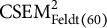 ${\mathrm{CSEM}}_{\mathrm{Feldt}(60)}^2$
. On test part
${\mathrm{CSEM}}_{\mathrm{Feldt}(60)}^2$
. On test part $k=1$
, individual 60 has sum score
$k=1$
, individual 60 has sum score ${x}_{+60.1}=1$
(the dot separates different indices). Given that test parts are individual items, the sum score equals the item score, that is,
${x}_{+60.1}=1$
(the dot separates different indices). Given that test parts are individual items, the sum score equals the item score, that is, ${x}_{+ ik}={x}_{ik}$
. Given
${x}_{+ ik}={x}_{ik}$
. Given ${x}_{+60}=9$
, the individual’s mean test-part score equaled
${x}_{+60}=9$
, the individual’s mean test-part score equaled ${\overline{x}}_{60}=1$
. The mean score for test part
${\overline{x}}_{60}=1$
. The mean score for test part $k=1$
equaled
$k=1$
equaled ${\overline{x}}_1=1.397$
. Because the test-part means have to add up to
${\overline{x}}_1=1.397$
. Because the test-part means have to add up to $9$
, the mean of the test part means is
$9$
, the mean of the test part means is $M=1.285$
. Using Equation (A.
2) for all test parts
$M=1.285$
. Using Equation (A.
2) for all test parts $k=1,\dots, 9$
, we obtained
$k=1,\dots, 9$
, we obtained ${\mathrm{CSEM}}_{\mathrm{Feldt}(i)}^2$
values for each of the 68 individuals with a sum score of
${\mathrm{CSEM}}_{\mathrm{Feldt}(i)}^2$
values for each of the 68 individuals with a sum score of $9$
, the average of which equaled
$9$
, the average of which equaled $\overline{\mathrm{CSEM}^{2}}_{\mathrm{Feldt}(i)}=4.7524$
. Then, for
$\overline{\mathrm{CSEM}^{2}}_{\mathrm{Feldt}(i)}=4.7524$
. Then, for ${X}_{+}=9,$ ${\widehat{\mathrm{CSEM}}}_{\mathrm{Feldt}}=\sqrt{4.7524}=2.18.$
Mollenkopf method. The Mollenkopf method serves as an introduction to the Mollenkopf–Feldt method. Mollenkopf (Reference Mollenkopf1949) suggested predicting the squared difference of sum scores on test halves,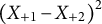 ${\left({X}_{+1}-{X}_{+2}\right)}^2$
, by a polynomial regression function with intercept
${\left({X}_{+1}-{X}_{+2}\right)}^2$
, by a polynomial regression function with intercept ${\beta}_0$
and regression coefficients
${\beta}_0$
and regression coefficients ${\beta}_1,\dots, {\beta}_q$
. Feldt and Qualls (Reference Feldt and Qualls1996) adjusted the method for essentially
${\beta}_1,\dots, {\beta}_q$
. Feldt and Qualls (Reference Feldt and Qualls1996) adjusted the method for essentially $\tau$
equivalent test halves by adding the adjustment factor of half-test means as
$\tau$
equivalent test halves by adding the adjustment factor of half-test means as ${\overline{X}}_1-{\overline{X}}_2$
. Next, subjecting the squared difference scores to a polynomial regression of order
${\overline{X}}_1-{\overline{X}}_2$
. Next, subjecting the squared difference scores to a polynomial regression of order $q$
with residual
$q$
with residual $\varepsilon$
gives the following squared
$\varepsilon$
gives the following squared ${\mathrm{CSEM}}_{\mathrm{Moll}}$
adjusted by Feldt and Qualls (Reference Feldt and Qualls1996):
${\mathrm{CSEM}}_{\mathrm{Moll}}$
adjusted by Feldt and Qualls (Reference Feldt and Qualls1996):
 $$\begin{align}{\mathrm{CSEM}}_{\mathrm{Moll}}^2= \mathbb{E} \left\{{\left(\left({X}_{+1}-{X}_{+2}\right)-\left({\overline{X}}_{+1}-{\overline{X}}_{+2}\right)\right)}^2\right\}={\beta}_0+{\beta}_1{X}_{+}+{\beta}_2{X}_{+}^2+\dots +{\beta}_q{X}_{+}^q.\end{align}$$
For the ADD data, we first calculated the squared raw difference scores ${\left(\left({X}_{+1}-{X}_{+2}\right)-\left({\overline{X}}_{+1}-{\overline{X}}_{+2}\right)\right)}^2$
, and then predicted these using a polynomial regression model with the sum scores
${\left(\left({X}_{+1}-{X}_{+2}\right)-\left({\overline{X}}_{+1}-{\overline{X}}_{+2}\right)\right)}^2$
, and then predicted these using a polynomial regression model with the sum scores ${X}_{+}$
as the predictors with different powers. Choosing a third-degree polynomial,
${X}_{+}$
as the predictors with different powers. Choosing a third-degree polynomial, $Y={\beta}_0+{\beta}_1{X}_1+{\beta}_2{X}_2+{\beta}_3{X}_3+\varepsilon,$
with
$Y={\beta}_0+{\beta}_1{X}_1+{\beta}_2{X}_2+{\beta}_3{X}_3+\varepsilon,$
with ${X}_2={X}_{+}^2$
and
${X}_2={X}_{+}^2$
and ${X}_3={X}_{+}^3$
, we obtained the estimates of the coefficients
${X}_3={X}_{+}^3$
, we obtained the estimates of the coefficients ${\beta}_0,\dots, {\beta}_3$
. If we now replace
${\beta}_0,\dots, {\beta}_3$
. If we now replace ${X}_{+}$
in the third-degree polynomial regression equation with the sum scores of the ADD data ranging from 0 to 36, and then take the square root of the resulting 36 values, we obtain the
${X}_{+}$
in the third-degree polynomial regression equation with the sum scores of the ADD data ranging from 0 to 36, and then take the square root of the resulting 36 values, we obtain the ${\mathrm{CSEM}}_{\mathrm{Moll}}$
estimates for the 36 possible scores for the ADD data.
${\mathrm{CSEM}}_{\mathrm{Moll}}$
estimates for the 36 possible scores for the ADD data.
Mollenkopf–Feldt method. The ${\mathrm{CSEM}}_{\mathrm{MF}}$
is a combination of
${\mathrm{CSEM}}_{\mathrm{MF}}$
is a combination of ${\mathrm{CSEM}}_{\mathrm{Moll}}$
and
${\mathrm{CSEM}}_{\mathrm{Moll}}$
and ${\mathrm{CSEM}}_{\mathrm{Feldt}}$
. Instead of splitting the test into halves, the test is split into
${\mathrm{CSEM}}_{\mathrm{Feldt}}$
. Instead of splitting the test into halves, the test is split into $K$
equal-length test parts, and the difference score for each part (following the Feldt method) is predicted by a polynomial regression (Feldt & Qualls, Reference Feldt and Qualls1996). Thus, the right-hand side of Equation (A.
2) is predicted by a regression function to further reduce the sampling error of the estimates and better approximate their population values (Feldt & Qualls, Reference Feldt and Qualls1996); that is,
$K$
equal-length test parts, and the difference score for each part (following the Feldt method) is predicted by a polynomial regression (Feldt & Qualls, Reference Feldt and Qualls1996). Thus, the right-hand side of Equation (A.
2) is predicted by a regression function to further reduce the sampling error of the estimates and better approximate their population values (Feldt & Qualls, Reference Feldt and Qualls1996); that is,
 $$\begin{align}{\mathrm{CSEM}}_{\mathrm{MF}}=\sqrt{d\times \frac{\sum \limits_{k=1}^K{\left\lceil \left({X}_{+ ik}-{\overline{X}}_i\right)-\left({\overline{X}}_k-M\right)\right\rceil}^2}{K-1}}=\sqrt{\beta_0+{\beta}_1{X}_{+}+{\beta}_2{X}_{+}^2+\dots +{\beta}_q{X}_{+}^q\;}.\end{align}$$
Estimating the ${\mathrm{CSEM}}_{\mathrm{MF}}$
values follows the same trajectory as the
${\mathrm{CSEM}}_{\mathrm{MF}}$
values follows the same trajectory as the ${\mathrm{CSEM}}_{\mathrm{Moll}}$
. For the ADD data, we split the test into nine parts coinciding with individual items. We then computed the sums of the difference scores for each part and fit a third-degree polynomial regression model. With the resulting regression coefficients, we computed the
${\mathrm{CSEM}}_{\mathrm{Moll}}$
. For the ADD data, we split the test into nine parts coinciding with individual items. We then computed the sums of the difference scores for each part and fit a third-degree polynomial regression model. With the resulting regression coefficients, we computed the ${\mathrm{CSEM}}_{\mathrm{MF}}$
values for each sum score. For example, for sum score
${\mathrm{CSEM}}_{\mathrm{MF}}$
values for each sum score. For example, for sum score ${x}_{+}=9$
, we found
${x}_{+}=9$
, we found ${\widehat{\mathrm{CSEM}}}_{\mathrm{MF}}=2.209$
.
${\widehat{\mathrm{CSEM}}}_{\mathrm{MF}}=2.209$
.
A.2.2 ANOVA method
We consider a repeated measures ANOVA with two main effects (items and subjects) and an interaction effect of items and subjects. The ${\mathrm{CSEM}}_{\mathrm{ANOVA}}=\sqrt{K\times \mathrm{M}{\mathrm{S}}_{K\times N}}$
, with
${\mathrm{CSEM}}_{\mathrm{ANOVA}}=\sqrt{K\times \mathrm{M}{\mathrm{S}}_{K\times N}}$
, with $\mathrm{M}{\mathrm{S}}_{K\times N}$
denoting the mean squares of the interaction effect, that is, the interaction between items and observations. Emons (Reference Emons, Van Der Ark, Emons and Meijer2023) described how this equation can be re-expressed using the intraclass correlation coefficient
$\mathrm{M}{\mathrm{S}}_{K\times N}$
denoting the mean squares of the interaction effect, that is, the interaction between items and observations. Emons (Reference Emons, Van Der Ark, Emons and Meijer2023) described how this equation can be re-expressed using the intraclass correlation coefficient $\mathrm{ICC}\left(3,K\right)$
(Shrout & Fleiss, Reference Shrout and Fleiss1979). The formula for the
$\mathrm{ICC}\left(3,K\right)$
(Shrout & Fleiss, Reference Shrout and Fleiss1979). The formula for the ${\mathrm{CSEM}}_{\mathrm{ANOVA}}$
uses
${\mathrm{CSEM}}_{\mathrm{ANOVA}}$
uses $J$
and the trace of the covariance matrix
$J$
and the trace of the covariance matrix ${\boldsymbol{\Sigma}}_{\mathbf{X}}$
, that is, the sum of the diagonal elements (i.e., the item variances), and equals
${\boldsymbol{\Sigma}}_{\mathbf{X}}$
, that is, the sum of the diagonal elements (i.e., the item variances), and equals
 $$\begin{align}{\mathrm{CSEM}}_{\mathrm{ANOVA}}=\sqrt{\frac{J}{J-1}\mathrm{tr}\left({\boldsymbol{\Sigma}}_{\mathbf{X}}\right)}.\end{align}$$
To obtain the ${\mathrm{CSEM}}_{\mathrm{ANOVA}}$
for a specific test score, we replace the trace of
${\mathrm{CSEM}}_{\mathrm{ANOVA}}$
for a specific test score, we replace the trace of ${\boldsymbol{\Sigma}}_{\mathbf{X}}$
for all individuals with the trace of the interitem covariance matrix of the individuals with a specific test score. For instance, for the ADD data, we find 68 participants with a sum score of
${\boldsymbol{\Sigma}}_{\mathbf{X}}$
for all individuals with the trace of the interitem covariance matrix of the individuals with a specific test score. For instance, for the ADD data, we find 68 participants with a sum score of ${x}_{+}=9$
, which means we estimate the covariance matrix of a subsample with 68 observations across 9 items and insert that into Equation (A.5). This yields a
${x}_{+}=9$
, which means we estimate the covariance matrix of a subsample with 68 observations across 9 items and insert that into Equation (A.5). This yields a ${\widehat{\mathrm{CSEM}}}_{\mathrm{ANOVA}}=2.20$
.
${\widehat{\mathrm{CSEM}}}_{\mathrm{ANOVA}}=2.20$
.
A.3 IRT-related CSEM methods
A.3.1 IRT dichotomous data method
To obtain a CSEM from an IRT model, we combine the error variability for a given latent variable value across the different items in the test. Let $P\left({X}_j|\theta \right)$
be shorthand for the probability of a positive response to item
$P\left({X}_j|\theta \right)$
be shorthand for the probability of a positive response to item $j$
,
$j$
, $P\left({X}_j=1|\theta \right)$
, given the latent variable
$P\left({X}_j=1|\theta \right)$
, given the latent variable $\theta$
. Using the 2PLM, one may estimate the
$\theta$
. Using the 2PLM, one may estimate the ${\mathrm{CSEM}}_{2\mathrm{PLM}}$
depending on latent variable
${\mathrm{CSEM}}_{2\mathrm{PLM}}$
depending on latent variable $\theta$
as
$\theta$
as
 $$\begin{align}{\mathrm{CSEM}}_{2\mathrm{PLM}}\left(\theta \right)=\sqrt{\sum \limits_{j=1}^JP\left({X}_j|\theta \right)\left(1-P\left({X}_j|\theta \right)\right)}.\end{align}$$
Probability $P\left({X}_j|\theta \right)$
is obtained by estimating a 2PLM and inserting the resulting estimates of location and discrimination parameters,
$P\left({X}_j|\theta \right)$
is obtained by estimating a 2PLM and inserting the resulting estimates of location and discrimination parameters, ${b}_j$
and
${b}_j$
and ${a}_j$
into the 2PLM function for each latent variable score:
${a}_j$
into the 2PLM function for each latent variable score:
 $$\begin{align}P\left({X}_j=1|\theta \right)=\frac{\exp \left[{a}_j\left(\theta -{b}_j\right)\right]}{1+\exp \left[{a}_j\left(\theta -{b}_j\right)\right]}.\end{align}$$
Equation (A.6) provides the score-related ${\mathrm{CSEM}}_{2\mathrm{PLM}}\left(\theta \right)$
, and a
${\mathrm{CSEM}}_{2\mathrm{PLM}}\left(\theta \right)$
, and a ${\mathrm{CSEM}}_{2\mathrm{PLM}}\left(\theta \right)$
value is obtained for as many
${\mathrm{CSEM}}_{2\mathrm{PLM}}\left(\theta \right)$
value is obtained for as many $\theta$
values as one deems useful for the application at hand. Interestingly, different values of the latent variable imply different real-valued sum scores (a result we will ignore for simplicity’s sake, but nevertheless providing useful results), hence, estimating different
$\theta$
values as one deems useful for the application at hand. Interestingly, different values of the latent variable imply different real-valued sum scores (a result we will ignore for simplicity’s sake, but nevertheless providing useful results), hence, estimating different ${\mathrm{CSEM}}_{2\mathrm{PLM}}\left(\theta \right)$
values provide the user with a SEM conditional on a real-valued sum score.
${\mathrm{CSEM}}_{2\mathrm{PLM}}\left(\theta \right)$
values provide the user with a SEM conditional on a real-valued sum score.
Technical details are the following. The estimated item parameters may be obtained using the R-package mirt (Chalmers, Reference Chalmers2012). The latent variable values may either be the estimated values, or the researcher may choose plausible values, such as $\theta =-5,-4.9,-4.8,\dots, 5$
, depending on the norming of the latent variable in the estimation procedure. We used values
$\theta =-5,-4.9,-4.8,\dots, 5$
, depending on the norming of the latent variable in the estimation procedure. We used values $\theta =-5,\dots, 5$
with increments of
$\theta =-5,\dots, 5$
with increments of $0.1$
, thus obtaining
$0.1$
, thus obtaining $101$
values. Plugging a
$101$
values. Plugging a $\theta$
value into Equation (A.7), for each item we obtained
$\theta$
value into Equation (A.7), for each item we obtained $P\left({X}_j|\theta \right)$
. Adding these probabilities yielded a real-valued sum score for that
$P\left({X}_j|\theta \right)$
. Adding these probabilities yielded a real-valued sum score for that $\theta$
value. This way, we obtained
$\theta$
value. This way, we obtained $101$
values for
$101$
values for ${\mathrm{CSEM}}_{2\mathrm{PLM}}$
for latent variable scores along the real-valued sum-score scale.
${\mathrm{CSEM}}_{2\mathrm{PLM}}$
for latent variable scores along the real-valued sum-score scale.
A.3.2 IRT polytomous data method
For polytomous data, we suggest the GRM. The error variance of a single item is given by
 $$\begin{align}{\sigma}_{E_{X_j}}^2=\sum \limits_x{\left(x-\mathbb{E}\left({X}_j\right)\right)}^2P\left({X}_j=x|\theta \right),\end{align}$$
hence, adding these item variances across $J$
items provides
$J$
items provides
 $$\begin{align}{\mathrm{CSEM}}_{\mathrm{GRM}}=\sqrt{\sum_{j=1}^J{\sigma}_{E_{X_j}}^2}.\end{align}$$
Expectation $\mathbb{E}\left({X}_j\right)$
denotes the mean of item
$\mathbb{E}\left({X}_j\right)$
denotes the mean of item ${X}_j$
and is given by
${X}_j$
and is given by $\mathbb{E}\left({X}_j\right)={\sum}_xx\;P\left({X}_j=x|\theta \right)$
; here, summation is done across all item scores, for example,
$\mathbb{E}\left({X}_j\right)={\sum}_xx\;P\left({X}_j=x|\theta \right)$
; here, summation is done across all item scores, for example, $x=0,\dots, 4$
. Probability
$x=0,\dots, 4$
. Probability $P\left({X}_j=x|\theta \right)$
is the probability of scoring
$P\left({X}_j=x|\theta \right)$
is the probability of scoring $x$
on item
$x$
on item $j$
, given by
$j$
, given by
 $$\begin{align}P\left({X}_j=x|\theta \right)=P\left({X}_j\ge x|\theta \right)-P\left({X}_j\ge x+1|\theta \right).\end{align}$$
Let parameter ${a}_j$
be the discrimination parameter for item
${a}_j$
be the discrimination parameter for item $j$
, and
$j$
, and ${b}_{jx}$
the location parameter for item
${b}_{jx}$
the location parameter for item $j$
and item score
$j$
and item score $x$
. Probability
$x$
. Probability $P\left({X}_j\ge x|\theta \right)$
is modeled by means of the GRM as
$P\left({X}_j\ge x|\theta \right)$
is modeled by means of the GRM as
 $$\begin{align}P\left({X}_j\ge x|\theta \right)=\frac{\exp \left[{a}_j\left(\theta -{b}_{jx}\right)\right]}{1+\exp \left[{a}_j\left(\theta -{b}_{jx}\right)\right]}.\end{align}$$
These probabilities are used to obtain the probability $P\left({X}_j=x|\theta \right)$
(Equation (A.10)).
$P\left({X}_j=x|\theta \right)$
(Equation (A.10)).
For the ADD data, we estimated a GRM using the R package mirt (Chalmers, Reference Chalmers2012). The probabilities in Equation (A.10) were estimated for 101 values $\theta =-5,\dots, 5$
with
$\theta =-5,\dots, 5$
with $0.1$
increments, using the estimates of the location and discrimination parameters for the item under consideration. For a specific
$0.1$
increments, using the estimates of the location and discrimination parameters for the item under consideration. For a specific $\theta$
value, computing expected item scores,
$\theta$
value, computing expected item scores, $\mathbb{E}\left({X}_j\right)$
, and adding across the
$\mathbb{E}\left({X}_j\right)$
, and adding across the $J$
items yielded the real-valued sum score. We thus obtained
$J$
items yielded the real-valued sum score. We thus obtained $101$
values of
$101$
values of ${\mathrm{CSEM}}_{\mathrm{GRM}}$
for real-valued sum scores, ranging from
${\mathrm{CSEM}}_{\mathrm{GRM}}$
for real-valued sum scores, ranging from ${X}_{+}=0.015$
to
${X}_{+}=0.015$
to ${X}_{+}=35.41$
.
${X}_{+}=35.41$
.
A.4 Binomial SEM approaches for dichotomous data
Lord method. Let ${X}_c$
denote the number of correct answers to the items. The CSEM is given by
${X}_c$
denote the number of correct answers to the items. The CSEM is given by
 $$\begin{align}{\mathrm{CSEM}}_{\mathrm{BL}}=\sqrt{\frac{X_c\left(J-{X}_c\right)}{J-1}}.\end{align}$$
Replacing ${X}_c$
with a realization
${X}_c$
with a realization ${x}_c$
gives the
${x}_c$
gives the $\kern0.24em {\mathrm{CSEM}}_{\mathrm{BL}}$
for the subgroup having
$\kern0.24em {\mathrm{CSEM}}_{\mathrm{BL}}$
for the subgroup having ${x}_c$
items correct.
${x}_c$
items correct.
Keats method. The elate is given by
 $$\begin{align}{\mathrm{CSEM}}_{\mathrm{BK}}=\sqrt{\left(\frac{X_c\left(J-{X}_c\right)}{J-1}\right)\left(\frac{1-\rho }{1-{KR}_{21}}\right)}.\end{align}$$
Parameter $\rho$
denotes an appropriate reliability estimate, such as coefficient
$\rho$
denotes an appropriate reliability estimate, such as coefficient $\alpha$
. Coefficient
$\alpha$
. Coefficient $\mathrm{K}{\mathrm{R}}_{21}$
(Kuder & Richardson, Reference Kuder and Richardson1937) is an approximation to coefficient
$\mathrm{K}{\mathrm{R}}_{21}$
(Kuder & Richardson, Reference Kuder and Richardson1937) is an approximation to coefficient $\alpha$
(Cronbach, Reference Cronbach1951), stemming from the days that computers did not exist, and shortcut approximations were of great value to realize computations that would otherwise place too much burden on the researcher. Again, to obtain the
$\alpha$
(Cronbach, Reference Cronbach1951), stemming from the days that computers did not exist, and shortcut approximations were of great value to realize computations that would otherwise place too much burden on the researcher. Again, to obtain the ${\mathrm{CSEM}}_{\mathrm{BK}}$
values, one computes the formula in Equation (A.
1
3) for any number of correct items
${\mathrm{CSEM}}_{\mathrm{BK}}$
values, one computes the formula in Equation (A.
1
3) for any number of correct items ${x}_c.$
Generalized Lord’s method. Let $K$
be the number of subtests;
$K$
be the number of subtests; ${c}_k$
the number of items in subtest
${c}_k$
the number of items in subtest $k$
; and
$k$
; and ${X}_{ik}$
the sum score (number of correct responses) of individual
${X}_{ik}$
the sum score (number of correct responses) of individual $i$
on subtest
$i$
on subtest $k$
. The SEM equals
$k$
. The SEM equals
 $$\begin{align}{\mathrm{CSEM}}_{BL2(i)}=\sqrt{\sum \limits_{k=1}^K\frac{X_{ik}\left({c}_k-{X}_{ik}\right)}{c_k-1}}.\end{align}$$
Equation (A.14) provides a SEM for each individual. Averaging over individuals with the same sum score, one obtains the ${\mathrm{CSEM}}_{\mathrm{BL}2}$
values (similar to the
${\mathrm{CSEM}}_{\mathrm{BL}2}$
values (similar to the ${\mathrm{CSEM}}_{\mathrm{Feldt}}$
).
${\mathrm{CSEM}}_{\mathrm{Feldt}}$
).
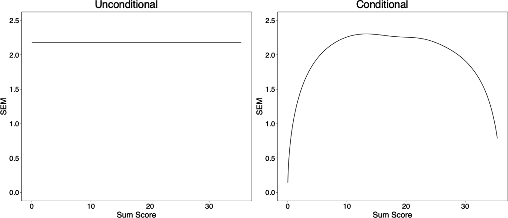
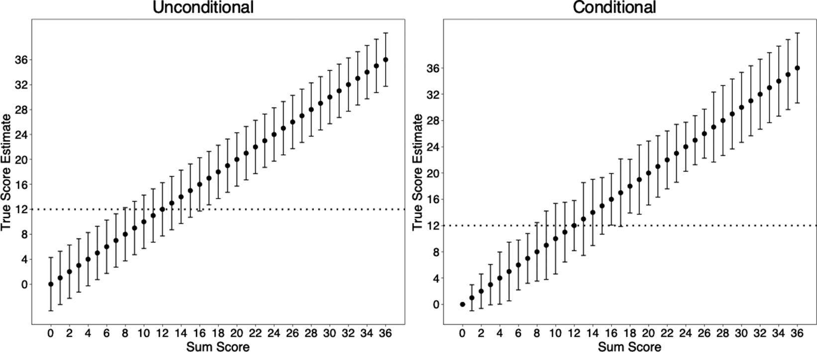
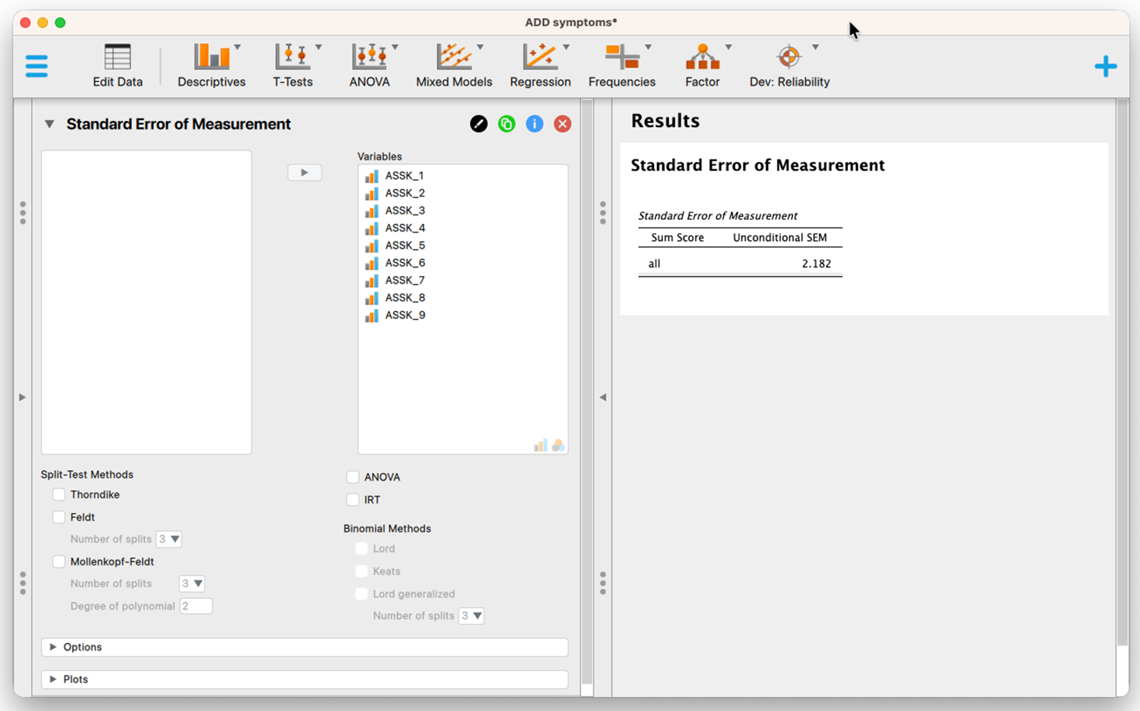
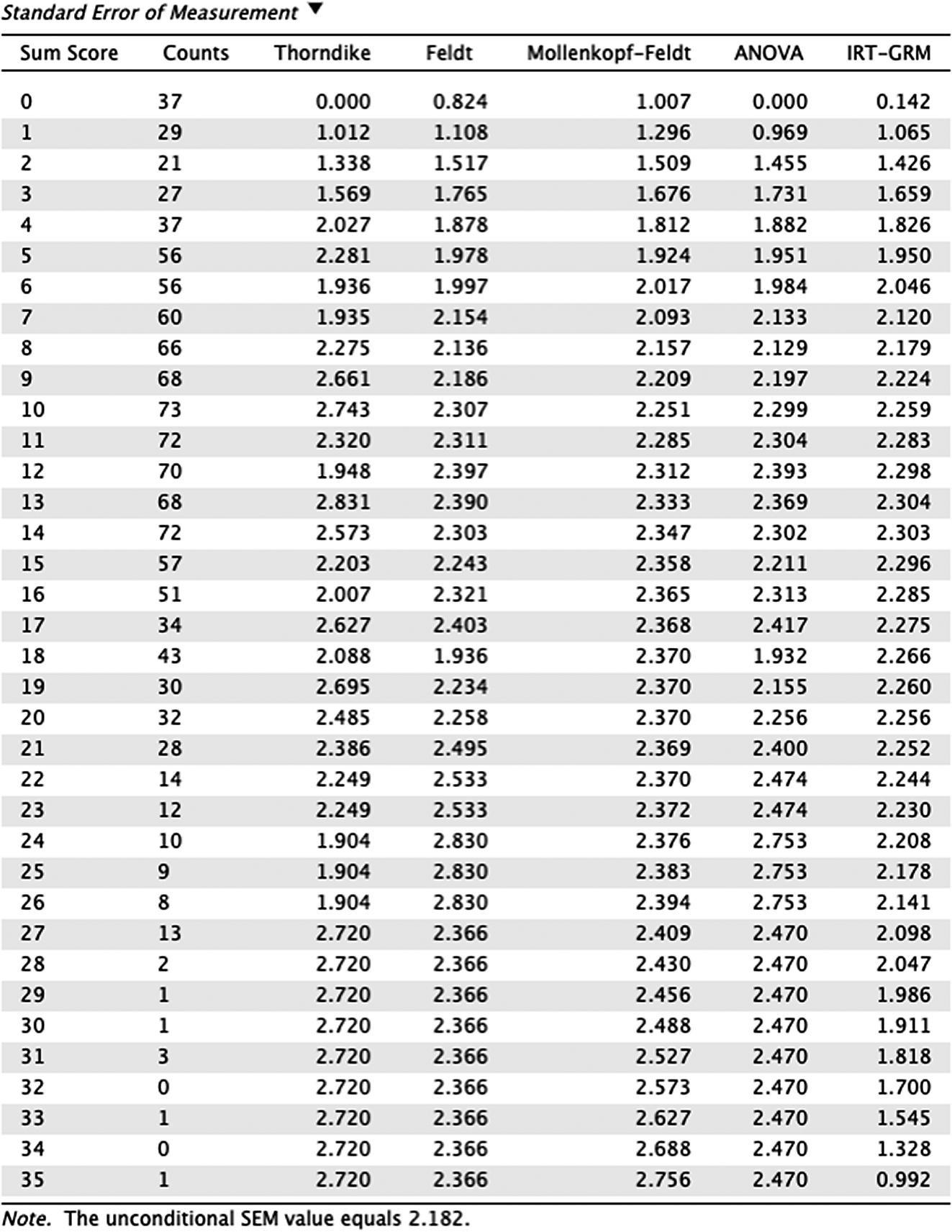

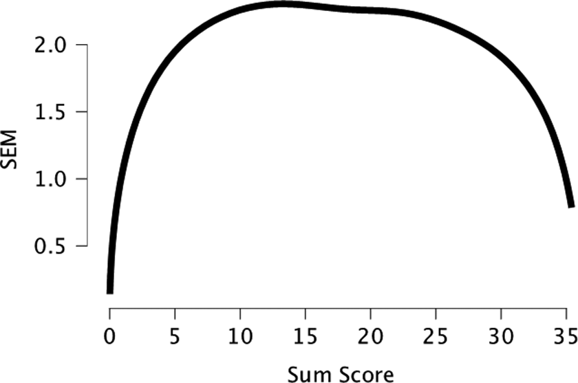
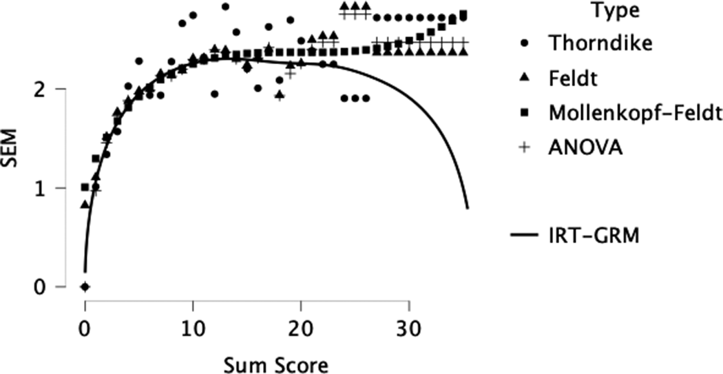
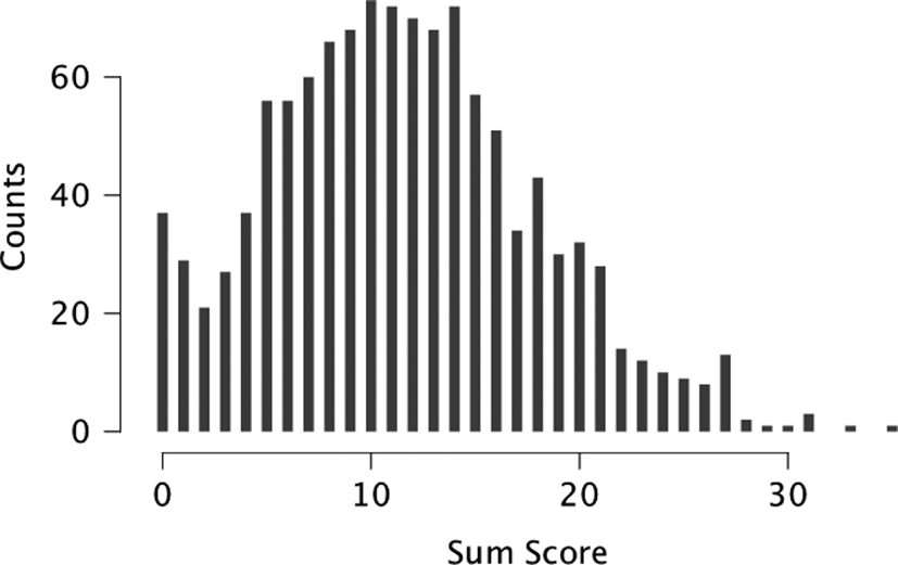

 Open access

